2. The rise and fall of DMG and DRFEFootnote ¹

The shutdown of DMG and DRFE in 2008 was one of Colombia’s most well-known financial scandals. It exposed weaknesses in government oversight and highlighted the social and economic conditions that enabled Ponzi schemes to flourish. Together, these companies attracted over half a million investors and collected funds equal to 1.2% of Colombia’s GDP – equivalent to 22% of Bancolombia’s total deposits at the time (Bancolombia was the country’s largest bank).

DMG was founded in 2003 in La Hormiga, Putumayo, in southwestern Colombia, by David Murcia Guzmán, a high school graduate with experience in multi-level marketing. DMG’s business model promised very high returns – between 50% and 300% in six months – and sold prepaid cards that customers could use to buy discounted goods in the future. This way, they avoided being classified and supervised as a financial institution.

DMG expanded to 62 towns and later reached Panama, Venezuela, and Ecuador, and invested in shipping, media, and other sectors. A key moment came in 2006 with the launch of the “Body Channel,” a TV station attended by celebrities. This brought national attention and led to investigations. The Financial Superintendency (Superfinanciera – the agency that supervises financial institutions) warned that DMG was not authorized to take public deposits. The UIAF (Unidad de Información y Análisis Financiero – Colombia’s financial intelligence agency) investigated suspicious transactions linked to the Body Channel.

DMG resisted government actions through legal challenges, political connections, and public relations campaigns. Murcia funded politicians and lobbied Congress to legalize his business. In 2007, Superfinanciera ordered DMG to shut down, but Murcia appealed in local courts and reopened under a new company name. By early 2008, more agencies became involved, including DIAN (Colombia’s tax agency) and the Superintendencia de Sociedades (Supersociedades – the supervisor of large non-financial companies). Murcia’s luxurious lifestyle – with expensive cars and a private jet – continued to attract investors.

In November 2008, the Colombian government declared a State of Social Emergency, giving regulators more authority. DMG was shut down, and Murcia was arrested in Panama in 2009. He was extradited to the United States and sentenced to nine years in prison, followed by a 22-year sentence in Colombia, which he is still serving as of 2025. DMG’s asset liquidation returned very little to investors. Since the company was not a legal financial institution, deposits were not guaranteed. The recovered funds were distributed equally among investors, regardless of the amount each had invested. The scandal revealed networks of corruption involving politicians, journalists, and even links to guerrilla and paramilitary groups. DMG’s origins in Putumayo’s coca boom illustrated the connection between illegal economies and financial fraud.

DRFE (Dinero Rápido, Fácil y Efectivo – Fast, Easy, and Cash Money) was founded later than DMG, in 2007, by Pastor Carlos Alfredo Suárez in Pasto, Nariño. DRFE expanded rapidly, opening offices in 69 towns and reaching Ecuador, and promised monthly returns of 80% to 150%, also funded by new investor deposits. Though smaller than DMG, DRFE followed a similar path and operated mainly in Nariño and Putumayo.

After the emergency declaration in November 2008, DRFE was shut down along with DMG. Suárez was arrested and sentenced in 2011 to seven years in prison and a large fine. The recovered funds were returned to investors, with each receiving an equal amount. As in the case of DMG, the liquidation of DRFE resulted in investors recovering only a small portion of their capital: customers got back less than 5% of the average investment.

A common question is why so many investors were not alarmed by the extremely high promised returns. At the time, formal financial institutions were offering annual interest rates of 8% to 10% for similar short-term deposits. As in other scams, the reasons varied. Some investors feared missing out, others believed the leaders were skilled investors, and some – as shown in this paper – used their financial knowledge to try to outsmart others. Overall, low education, poor financial literacy, and weak government institutions made Colombia a fertile ground for these scams. As Rodríguez-Pinilla et al. (Reference Rodríguez-Pinilla, Eduardo Castellanos-Rodríguez, López-Rodríguez and Esguerra-Umaña2024) emphasize, only 16.4% of respondents in a representative survey answered the three classical financial literacy questions correctly.Footnote ²

3. Data and stylized facts

Our analysis draws on two primary data sources. The first is an administrative dataset compiled by the auditor’s office appointed by the Colombian government following the shutdown of the two Ponzi schemes at the end of 2008. For each identified customer, the dataset records the total amount invested in the schemes (which we refer to as deposits) and the final balance at the time of the shutdown. The final balance reflects the net position of each investor vis-à-vis the firms at that point in time – that is, the total amount invested, net of withdrawals, purchases, and any returns or bonuses credited by the schemes.

We use this information to construct our main dependent variable: an indicator equal to one if the final balance is strictly negative Footnote ³ – that is, if the investor made a profit at the time of the shutdown – and zero otherwise. If an individual made multiple deposits over time, the dataset aggregates them into a single total deposit figure, without providing information on the timing of deposits or withdrawals. Importantly, the dataset does not include any information on investor characteristics beyond these financial outcomes.

The second data source is the SISBEN survey, a large-scale administrative database managed by the Colombian government to support the targeting of social programs. The survey includes individual-and household-level socioeconomic characteristics such as education, age, gender, household composition, and asset ownership. We use data from the second wave of SISBEN, conducted between 2003 and 2007, which collected information on approximately 32.5 million individuals nationwide. For reference, Colombia’s total population in 2007 was 43.9 million. At the time, this dataset covered nearly two-thirds of the population but excluded high-income households, as it was not designed to collect data from this segment (see Hofstetter et al. (Reference Hofstetter, Mejía, Rosas and Urrutia2018) for more details). Accordingly, results should be interpreted with the caveat that the sample is representative primarily of low-and middle-income households.

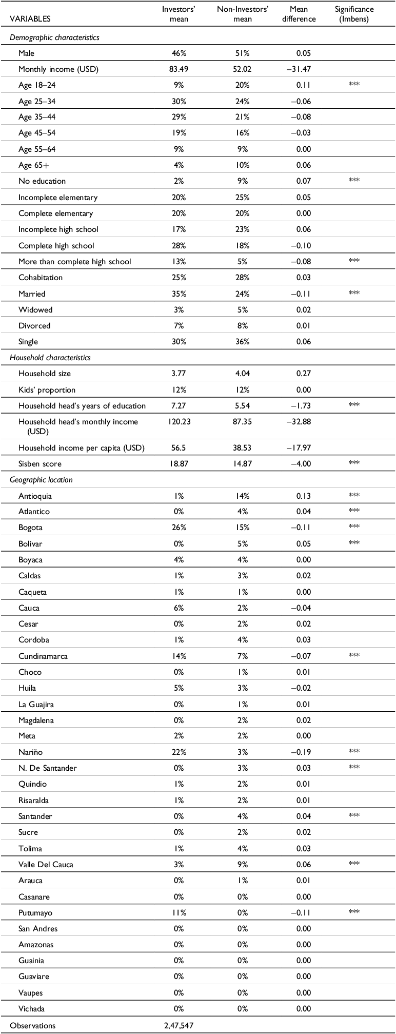
In Table 1, we report descriptive statistics on several socioeconomic characteristics of investors and of the overall population covered by the SISBEN survey for which we have data across all relevant variables, using the merged datasets.Footnote ⁴ We restrict the samples to individuals aged 18 and older.Footnote ⁵ The table presents the mean values of selected characteristics for investors and compares them to the corresponding means for the general adult population.

Table 1. Descriptive statistics. Investors and non-investors

The table reports the results of a two-sample t-test of equality of means, assuming equal variances. Column 1 presents the mean for investors, Column 2 the mean for non-investors, and Column 3 the mean difference between the two groups. Column 4 shows the significance level based on the Imbens Statistic, defined as the ratio of the mean difference to its standard error. In this context, a difference is considered statistically meaningful when the absolute value of the statistic is greater than 0.25, a rule that adjusts for the effect of sample size. All monetary variables are reported in USD, using the average exchange rate of November 2008.

Aside from some differences in geographic origin, investors also tend to be more educated than the general population. The proportion of investors without formal education is significantly lower – by 7 percentage points – while the share of those with post-secondary education is notably higher, by 8 percentage points. Moreover, investors are more likely to reside in households with higher overall educational attainment. In terms of the age distribution, individuals aged 18 to 24 are underrepresented among investors. Additionally, investors exhibit a higher average likelihood of being married and have better (higher) SISBEN scores – the index used by the Colombian government to determine eligibility thresholds for different social programs.Footnote ⁶ Finally, investors are disproportionately concentrated in Bogotá, Nariño, Cundinamarca, and Putumayo, where their mean shares exceed those in the general population by several percentage points. In contrast, they are underrepresented in departments such as Antioquia, Atlántico, Bolívar, Santander, and Valle del Cauca.

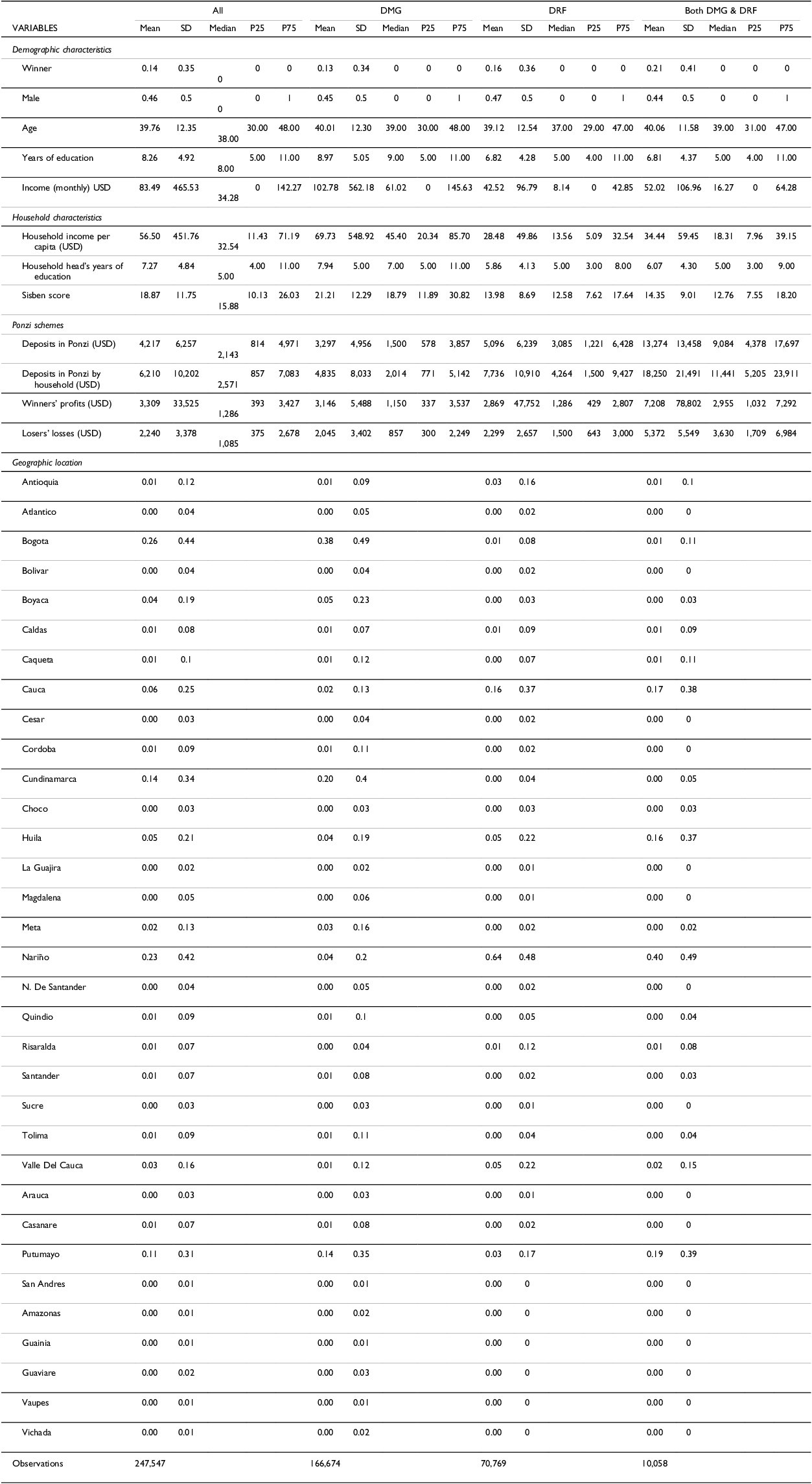
Table 2 splits investors into three groups: those who invested only in DMG, only in DRFE, and those who participated in both schemes, and reports summary statistics for the main variables of interest. These provide useful benchmarks for interpreting the magnitude of the econometric estimates in the subsequent analysis.Footnote ⁷

Table 2. Descriptive statistics. Investors, by scheme

All monetary variables are reported in USD (not logs), using the average exchange rate of November 2008.

A first notable difference emerges in terms of profitability, as the average proportion of winners varies across investor groups: 13 percent among DMG-only investors, 16 percent among DRFE-only investors, and 21 percent among those who participated in both schemes. Beyond differences in profitability, DMG investors tend to have higher individual incomes and more years of education. They also reside in households with higher per capita income, and the heads of these households typically show greater educational attainment.

Consequently, DMG-only investors exhibit the highest average SISBEN score (21.2), followed by dual investors (14.3) and DRFE-only investors (13.9). This pattern reinforces the notion that DMG attracted relatively better-off individuals, both in terms of personal characteristics and household context. To contextualize these figures, it is important to note that eligibility for many social assistance programs in Colombia is determined by a household’s SISBEN score. The cut-off thresholds vary depending on the specific program. For instance, the main national social program at the time – Familias en Acción, a conditional cash transfer initiative – had SISBEN cut-off scores of 11 for urban households and 17.5 for rural households.

Finally, regarding the geographic distribution of investors. DMG-only participants are primarily located in Bogotá (37.7%), Cundinamarca (20.2%), and Putumayo (14.1%), indicating a relatively wider geographic dispersion, including a strong presence in both the capital and peripheral regions. In contrast, DRFE-only investors are heavily concentrated in the southwest of the country: nearly 90% reside in just four departments – Nariño (63.7%), Cauca (16.0%), Huila (5.2%), and Valle del Cauca (5.1%) – pointing to a much more localized participant base. A similar concentration is observed among dual investors, who are predominantly located in Nariño (39.8%), Putumayo (18.8%), Cauca (17.2%), and Huila (16.1%). These geographic patterns not only reflect the origin and regional expansion of the two schemes but also suggest important differences in how they spread and whom they reached, as the high regional concentration of DRFE and dual investors stands in contrast to the broader footprint of DMG.

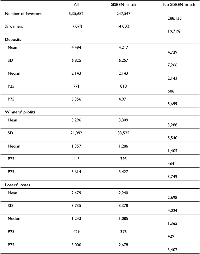
While there were more than half a million participants in the Ponzi scheme, less than half could be merged with demographics and are therefore included in the analysis. Hence, while the core analysis in this paper focuses on investors who could be merged with the SISBEN survey and for whom we have socioeconomic information, it is informative to compare this subsample to the broader population of scheme participants for whom only administrative data are available. Table 3 summarizes the main differences in balances, deposits, and profitability (i.e., being a “winner”) between the included and excluded groups. This comparison helps contextualize the external validity of our findings and offers insights into the broader impact of the Ponzi schemes’ collapse.

Table 3. Descriptive statistics. Investors, by matching situation

All monetary variables (Deposits, Winners’ profits, and Losers’ losses) are expressed in U.S. dollars (USD), converted using the average COP/USD exchange rate of November 2008. Deposits refer to the original invested capital, while winners’ profits and losers’ losses correspond to the final balance relative to the initial investment. Summary statistics are reported for the full sample, as well as separately for investors matched and not matched to SISBEN records. The proportion of winners is calculated as the share of investors with negative final balances.

Across the full set of investors, individuals not matched to SISBEN records tend to have larger investments and worse financial outcomes at the time of the shutdown. Their average deposit size is approximately $500 higher than that of included investors, profits are around $20 lower, and losses are about $450 higher. Despite these differences, the overall incidence of winners – those with negative net balances at shutdown – is higher for the unmatched investors, with a 5.71% lower share among the matched group. Despite these discrepancies, the general patterns of heterogeneity observed in the SISBEN-matched sample appear consistent with those in the unmatched group: higher deposits are associated with greater losses, and the incidence of winners remains relatively low across the board.

4. Empirical model and baseline results

We estimate multivariate probit models to analyze the likelihood that an investor made a profit by the time the government shut down the two Ponzi schemes. Our dependent variable, $ {W}_{i}$ , is a binary indicator equal to one if investor i made a profit (i.e., was a “winner”), and zero otherwise.Footnote ⁸ The probability of being a winner is modeled as a function of a set of socioeconomic characteristics of the investor and their household ( $ {X}_{i}$ ), as well as the state (departamento) of residence, captured by a full set of state fixed effects ( $ {F}_{s}$ ). Formally, our baseline specification is given by:

(1) $$ {P\left({\mathrm{W}}_{\mathrm{i}}=1|{\mathrm{X}}_{\mathrm{i}},{\mathrm{F}}_{\mathrm{s}}\right)=\Phi \left(\mathrm{\beta }{\mathrm{X}}_{\mathrm{i}}+{\mathrm{F}}_{\mathrm{s}}+{\mathrm{\varepsilon }}_{\mathrm{i}}\right)}$$

where $ \mathrm{\Phi }\left(\cdot \right)$ denotes the cumulative distribution function of the standard normal distribution, and $ {\varepsilon }_{i}$ is an idiosyncratic error term.

In Table 4, we report the estimated coefficients ( $ \beta $ ) as marginal effects on the probability of being a winner. For continuous variables, marginal effects are evaluated at their sample means; for binary variables, they represent the discrete change in predicted probability when moving from 0 to 1. We also report predicted probabilities of making a profit at the 10th and 90th percentiles for selected continuous regressors, holding all other covariates at their sample means. All specifications are estimated using robust standard errors clustered at the district level.

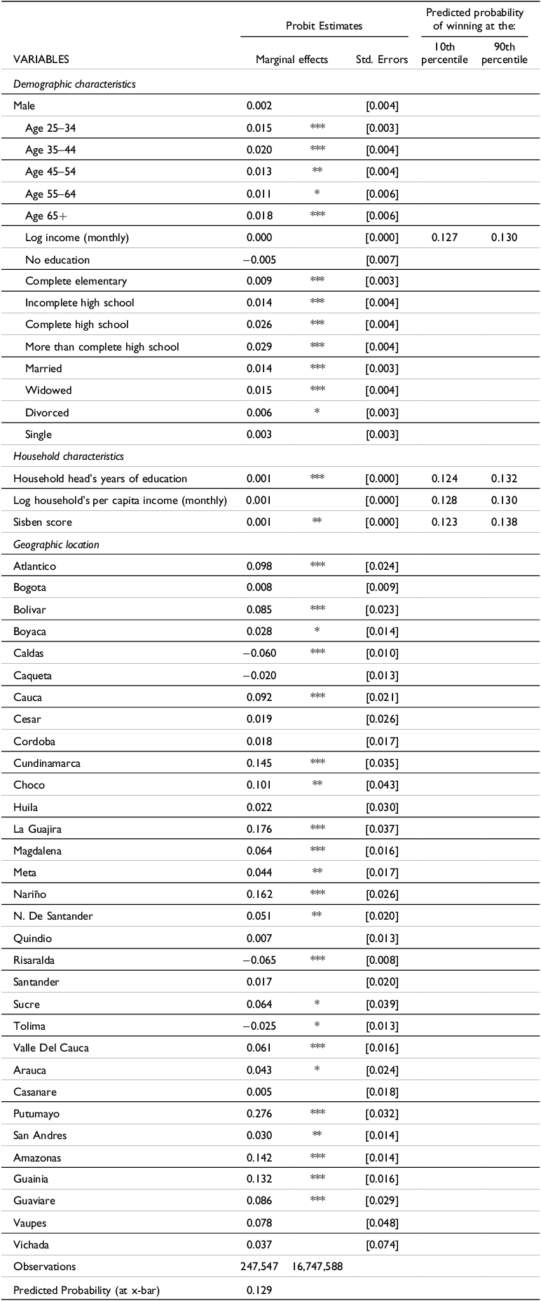
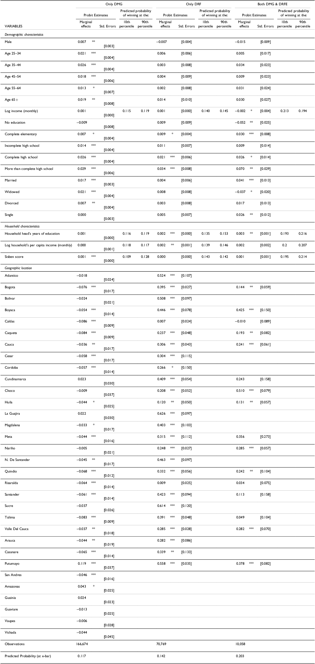
Table 4. Probability of making a profit. Results based on a probit model. The dependent variable is a dummy equal to one if the investor made a profit, and zero otherwise

***p < 0.01, **p < 0.05, p < 0.10. Standard errors are clustered at the municipal level. The dependent variable takes the value of 1 if the investor made a profit from investing in the Ponzi schemes, and 0 otherwise. The dummy variable for state1 (Antioquia) is dropped to avoid collinearity. Likewise, the comparison category for marital status is Cohabitation. The omitted age category is 18–24 years, and the omitted education category is incomplete elementary education. Variables of monthly income and household per capita income are expressed in natural logarithms using the ln(1 + x) transformation. If the head of the household was not an investor but a minor in the household was, the household head is assigned the balance and capital of the minor. Marginal effects are calculated at the mean; for discrete variables, they represent the change from 0 to 1.

We begin our analysis by examining the role of education. Prior work in the financial literacy literature (e.g., Lusardi and Mitchell Reference Lusardi and Mitchell2014) has found that people without a college education are less likely to grasp financial concepts and that numeracy is especially lacking among those with low educational attainment. That is, the years of education that we observe in our sample should be positively correlated with financial literacy, which we do not observe. This relationship has been recently corroborated in Colombia by Rodríguez-Pinilla et al. (Reference Rodríguez-Pinilla, Eduardo Castellanos-Rodríguez, López-Rodríguez and Esguerra-Umaña2024), who document a positive correlation between education and financial literacy. In the absence of direct measures of financial knowledge in our dataset, we use completed education levels as a proxy.

The date of the shutdown of the schemes was not public information, and, by and large, for most of the population, it came as a surprise. Nevertheless, the success of the two pyramids and the government’s suspicions that they were illegally taking deposits had been an important story in the national media for some time. Investors with higher levels of education may have been better positioned to interpret these signals, assess the risk of collapse or intervention, and withdraw their funds in a timely manner – thus increasing their chances of making a profit.

To explore this hypothesis, we categorize education into discrete levels based on completed schooling and estimate their association with the probability of being a winner. As shown in Table 4, relative to investors with incomplete elementary education (the reference group), the probability of making a profit increases monotonically with each successive education level. Completing elementary school is associated with a 0.9 percentage point increase in the likelihood of being a winner, while completing high school is associated with a 2.6 percentage point increase. The largest effect is observed among individuals with education beyond high school, who are almost 3.0 percentage points more likely to realize a profit compared to those with incomplete elementary education. Note that these results control for the investors’ age, whose role we analyze below. These results point to non-linear returns to education in terms of financial outcomes. Gains are relatively modest at lower levels of attainment but increase sharply for those completing secondary education and beyond. This pattern is consistent with the findings in the literature and supports the idea that higher education not only improves cognitive skills but also enhances the ability to process complex and uncertain financial information.

A related finding is the positive association between the education of the household head and the probability that the investor made a profit. This result aligns with prior evidence in the financial literacy literature. Lusardi and Mitchell (Reference Lusardi and Mitchell2014) highlight how individuals’ financial literacy is positively correlated with the educational attainment of their parents or household heads, reflecting both direct knowledge transmission and shared financial environments. Additionally, the household finance literature has found that less educated households are more prone to financial mistakes and suboptimal portfolio choices (Calvet et al. Reference Calvet, Campbell and Sodini2007, 2009). Our results are consistent with these findings. Quantitatively, moving from the 10th to the 90th percentile of the household head’s education distribution increases the predicted probability of being a winner from 12.4 percent to 13.2 percent, holding all other covariates at their means. The direction and consistency of the effect underscore the importance of household-level educational background in shaping financial outcomes.

That the young have low financial literacy levels, and the elderly are the target of financial predators, has been documented in the financial literacy literature (Agarwal et al. Reference Agarwal, Driscoll, Gabaix and Laibson2009; DeLiema et al. Reference DeLiema, Deevy, Lusardi and Mitchell2018; Karp and Wilson Reference Karp and Wilson2015; Lusardi and Mitchell Reference Lusardi and Mitchell2014). This literature highlights that financial literacy as a function of the age of individuals has an inverted U-shape: it is low for young individuals, then rises, reaches its peak at middle age, and then keeps declining as individuals grow older.

Our results are consistent with this pattern. In our baseline regression, we introduce age as a set of categorical variables, using individuals aged 18–24 as the reference group. As shown in Table 4, all age brackets between 25 and 64 are associated with a higher probability of making a profit relative to the youngest group. The effect peaks for investors aged 35–44, who are 2.0 percentage points more likely to be winners. The magnitude declines slightly for older age groups: the marginal effect is 1.3 percentage points for the 45–54 group and 1.1 percentage points for the 55–64 bracket. For individuals aged 65 and above, the marginal effect increases slightly but remains below the peak. Taken together, the coefficients suggest a non-linear relationship between age and investment outcomes, consistent with an inverted U-shape. Middle-aged investors appear more likely to have exited the schemes in time to make a profit, while younger and older investors were less successful in doing so – potentially reflecting lower financial literacy or a reduced ability to process and act upon complex financial signals.

As for gender differences, prior studies have highlighted persistent disparities in financial literacy between men and women. For instance, Lusardi and Mitchell (Reference Lusardi and Mitchell2008; 2011) report that women tend to be less financially literate than men, potentially affecting their investment decisions. In our setting, however, we find no statistically or economically meaningful gender differences in investment outcomes. As shown in Table 4, the marginal effect of being male on the probability of making a profit is small and statistically insignificant.

We next explore how socioeconomic status shapes financial outcomes. Campbell (Reference Campbell2006) and Calvet et al. (Reference Calvet, Campbell and Sodini2007, 2009) report that lower-income individuals are more likely to make financial mistakes. To examine this relationship, we consider three distinct indicators: (i) investors’ self-reported income, (ii) the per capita incomes of households, and (iii) the SISBEN score.

Among these different measures, only the SISBEN score displays a positive and statistically significant association with the probability of making a profit, suggesting that investors from households with better living conditions were more likely to exit the schemes before the shutdown, potentially reflecting better financial awareness or access to information. Specifically, moving from the 10th to the 90th percentile of the SISBEN score distribution increases the predicted probability of making a profit from 12.3 to 13.8 percent. This 12 percent increase underscores the role of household-level socioeconomic conditions in shaping financial decisions and outcomes during the operation of the schemes.

We conclude our analysis by examining the role of geographic location, as captured through state (departamento) fixed effects. One interpretation of regional variation in investor outcomes relates to timing – and, by extension, luck. We know that the main pyramid in our sample (DMG) started its operation in the remote state of Putumayo, in the southwest of the country. DRFE started in the neighboring state of Nariño. Several municipalities in these regions had more investors per capita than any other part of the country (Hofstetter et al. Reference Hofstetter, Mejía, Rosas and Urrutia2018).

While our dataset does not contain information on the dates of investments of each customer (only the final balances and capital are reported), it seems reasonable to assume that those living in Putumayo and Nariño were among the earliest participants in the schemes. In the structure of these Ponzi schemes, latecomers are more likely to lose than those investing and withdrawing early on. If geographic proximity to the schemes’ origins correlates with earlier entry, location may serve as a proxy for timing – and thus for luck.

Empirically, we find strong support for this hypothesis. As shown in Table 4, living in Putumayo is associated with a 28-percentage point increase in the probability of making a profit, the largest marginal effect among all variables in our model. Similarly, residing in Nariño increases the likelihood of being a winner by 16 percentage points. These effects remain highly significant even after controlling for a wide range of investor and household characteristics, including education and income.

While we interpret these results as consistent with a timing-based explanation, other mechanisms may also contribute to the observed geographic heterogeneity. One alternative is that proximity to the schemes’ main operations may have offered local investors better access to informal information channels – such as community networks or local media – about the sustainability or risks of the schemes. From this perspective, local residents may have been comparatively better informed and more responsive to signals indicating an impending collapse or potential government intervention.

More broadly, these fixed effects may capture unobserved regional differences in financial behavior, trust, or exposure to informal advice. For instance, Lusardi and Mitchell (Reference Lusardi and Mitchell2014) document regional differences in financial literacy. These could arise from differing policies promoted at the state level, heterogeneous financial literacy programs, and so on. Although Colombia is not a federal country – and national regulations and financial education policies are applied uniformly – local variation in implementation, media penetration, or social capital could still influence individual decision-making. Notably, our estimates control for a rich set of investor and household characteristics, including education and income, suggesting that the observed regional heterogeneity reflects deeper structural or informational differences not captured by standard socioeconomic indicators.

5. Scheme-specific results

In this section, we explore heterogeneity in investor outcomes by estimating the baseline probit model separately for participants in each of the two main Ponzi schemes: DMG and DRFE. This analysis is motivated by the fact that the schemes differed in important ways, including the socioeconomic profiles of their investors, their geographic reach, and the timing of their operations. DRFE participants were generally poorer, less educated, and more likely to belong to larger households with lower SISBEN scores, compared to those who invested in DMG. These differences are clearly reflected in our own data, as shown in Table 2. While our dataset does not include the precise timing of individual investments, the fact that DRFE was a relatively new scheme at the time of the shutdown suggests that most of its participants entered relatively late. By estimating separate models for each scheme, we can indirectly assess how investor characteristics and potential timing effects shaped the likelihood of making a profit. This disaggregation also provides a way to further evaluate the interpretation of the regional fixed effects in our baseline model, particularly because DMG and DRFE originated in different regions of the country.

We begin by examining the role of education across the three groups of investors. Estimates for each scheme are presented in Table 5. As in the baseline results for all investors (Table 4), we find a strong and generally increasing relationship between educational attainment and the probability of making a profit, although the magnitude and shape of this relationship vary by scheme. Among DMG-only investors, the positive association between education and profitability is both monotonic and statistically significant across almost all categories beyond the reference group (incomplete elementary education). Marginal effects increase with each successive education level, from 0.7 percentage points for completing elementary school to 2.9 percentage points for those with education beyond high school. This trend suggests that more educated investors in DMG were consistently more likely to exit the scheme in time to make a profit, consistent with the hypothesis that higher education correlates with greater financial awareness or responsiveness to risk signals.

Table 5. Probability of making a profit, by scheme. Results based on a probit model. The dependent variable is a dummy equal to one if the investor made a profit, and zero otherwise

***p < 0.01, **p < 0.05, p < 0.10. Standard errors are clustered at the municipal level. The dependent variable takes the value of 1 if the investor made a profit from investing in the Ponzi schemes, and 0 otherwise. The dummy variable for state1 (Antioquia) is dropped to avoid collinearity. Likewise, the comparison category for marital status is Cohabitation. The omitted age category is 18–24 years, and the omitted education category is incomplete elementary education. Variables of monthly income and household per capita income are expressed in natural logarithms using the ln(1 + x) transformation. If the head of the household was not an investor but a minor in the household was, the household head is assigned the balance and capital of the minor. Marginal effects are calculated at the mean; for discrete variables, they represent the change from 0 to 1.

In contrast, for DRFE-only investors, the pattern is less uniform. Only three education categories – complete elementary, complete high school, and more than high school – are significantly associated with higher profitability, with marginal effects of 0.9, 2.1 and 3.4 percentage points, respectively. The effects are comparable to those in DMG, but the lower education categories (complete elementary, incomplete high school) show either marginally significant associations at the 10% level or not statistically significant at all. This may reflect the more socioeconomically vulnerable profile of DRFE investors, for whom even basic educational thresholds may not translate into significantly better financial decision-making.

Among dual participants (those who invested in both DMG and DRFE), the education effects are again positive and increasing, though slightly larger in magnitude. For instance, having more than a high school education increases the probability of making a profit by 7.0 percentage points, nearly two-and-a-half times the effect observed in the full sample (2.9 percentage points). The large and significant coefficients in this subgroup suggest that education may have played an especially important role in enabling these investors to coordinate timing and risk across both schemes.

Taken together, these results confirm the aggregate finding of a non-linear, concave relationship between education and investment outcomes. The marginal benefit of education appears to grow as individuals cross key educational thresholds, particularly completing high school and entering post-secondary education.

We next examine how the probability of making a profit varies with investor age across the different pyramid schemes. In the aggregated results in Table 4, we observed an inverted U-shaped relationship: relative to the reference group (ages 18–24), marginal effects increase through the middle-age categories, peaking at ages 35–44 (2.0 percentage points), before gradually declining. This non-linear pattern is consistent with the life-cycle hypothesis in financial literacy, in which younger individuals lack experience, and older individuals may face cognitive decline.

When disaggregating by scheme, the DMG subsample largely mirrors this pattern. Marginal effects rise steadily with age and are statistically significant across all categories. Investors aged 35–44 are 2.6 percentage points more likely to make a profit than the youngest group, with slightly smaller effects in adjacent age brackets. The shape is consistent with a peak around middle age, reinforcing the idea that DMG investors with greater life experience – and potentially stronger financial literacy – were better positioned to anticipate the scheme’s collapse and withdraw in time.

In contrast, for the DRFE sample and among dual investors, there are no statistically significant age associations across any category. This may reflect a combination of factors: DRFE was a newer scheme at the time of the shutdown, allowing less scope for early withdrawal, and its investor base was generally more socioeconomically vulnerable. As a result, age alone may not have been a strong predictor of profitability in this group.

We now turn to the role of gender. In the aggregate analysis, being male is associated with a slightly higher likelihood of making a profit (0.2 percentage points), though the association was not statistically significant. When disaggregating by scheme, among DMG-only investors, the gender association becomes both statistically and economically meaningful: male investors are 0.7 percentage points more likely to make a profit, and the estimate is significant at the 5% level. This suggests that in the context of DMG – a scheme with broader reach and longer duration – gender-based differences in information processing, financial confidence, or responsiveness to risk may have played a role in shaping outcomes. In contrast, among DRFE-only investors and for dual investors, the marginal effect of being male is not statistically significant.

We continue the disaggregated analysis by examining the role of socioeconomic status, using the same three complementary indicators as before: household per capita income, the investor’s self-reported income, and the SISBEN score. In the aggregate analysis, only the latter was statistically significant, pointing to a positive association between household-level socioeconomic advantage and the likelihood of making a profit. Among DMG-only investors, SISBEN scores remain positively and significantly associated with the probability of making a profit. Moving from the 10^th to the 90^th percentile in the SISBEN score increases this probability by 1.9 percentage points. Investors from better-off households, whether due to higher economic standing or better access to information, were more likely to exit the scheme in time. In the DRFE-only group, the household per capita income has a statistically significant association (+0.2 percentage points). The SISBEN score, however, turns insignificant.

We now turn to the role of geographical location, captured by state (departamento) fixed effects. In the baseline specification, we interpreted the strong positive coefficients for Putumayo and Nariño as proxies for early entry into the pyramid schemes – consistent with the fact that DMG and DRFE, respectively, originated in those regions. The disaggregated estimates allow us to assess whether this interpretation holds when examining each scheme separately and assess potential alternative explanations, such as regional differences in financial literacy or information access.

Among DMG-only investors, the fixed effect for Putumayo remains positive and statistically significant, with a marginal effect of +12.0 percentage points relative to the reference category, Antioquia. This finding supports the interpretation that early exposure to DMG – likely due to geographic proximity to the scheme’s origin – conferred a timing advantage. Interestingly, Bogotá and Boyacá, despite being major hubs of DMG activity (37.7% and 5.4% of matched investors, respectively), exhibit negative fixed effects (−7.6 and −5.4 percentage points, respectively), suggesting that investors in these more urban regions were less likely to profit, potentially due to later entry as the scheme expanded nationally. Taken together, these patterns are consistent with the ‘luck’ hypothesis: early adopters, concentrated near the scheme’s point of origin, were more likely to profit, whereas those in geographically distant or later-adopting areas faced a higher risk of losses. The divergence in outcomes across regions with high investor density reinforces the view that timing, rather than purely regional socioeconomic conditions or informational advantages, played a central role in shaping investor returns within DMG.

For DRFE-only investors, location effects are even more pronounced. The marginal effect of residing in Nariño – where DRFE originated – is +24.8 percentage points. Several neighboring departments also display large and statistically significant marginal effects, including Cauca (+30.6 p.p.), Valle del Cauca (+28.5 p.p.), and Putumayo (+55.8 p.p.). Unlike the pattern observed for DMG, the strongest effects here are not confined to the scheme’s founding region but extend to a broader but highly concentrated geographic cluster. This attenuates the interpretation that luck through early entry alone explains the regional variation in outcomes. Instead, the magnitude and spread of these effects suggest that other mechanisms – such as informational spillovers, dense social networks, or local adaptation to the scheme’s operation – may have facilitated earlier or more strategic withdrawal. In this case, proximity to the scheme’s origin may still have mattered, but likely through channels beyond simple timing advantages.

Among dual investors, the pattern is broadly consistent with that observed for DRFE, though somewhat more geographically dispersed. The largest positive marginal effects are found in Putumayo (+37.8 p.p.), Nariño (+28.5 p.p.), Valle del Cauca (+28.2 p.p.), and Cauca (+24.1 p.p.) – all departments in the Southwest and that featured prominently in the operation of both schemes.

Taken together, these scheme-specific estimates strengthen the interpretation that regional location – especially proximity to the origin of the schemes – played a substantial role in investor outcomes. While we cannot fully disentangle whether these effects reflect luck in timing, better access to informal information, or regional adoption dynamics, the disaggregation reinforces the idea that early geographic exposure mattered significantly, particularly in DMG, for which the empirical evidence seems to support the ‘luck’ hypothesis.

6. Beyond profitability: Who invested in the scams?

Thus far, our analysis has focused on the probability of making a profit among those who invested in the pyramid schemes. While informative, this approach provides only a partial picture. Understanding who chose to invest in the first place is a necessary step toward a more complete characterization of the population affected by the scams. Participation in such schemes is itself a non-random outcome, likely influenced by a combination of socioeconomic characteristics, financial literacy, and possibly local context. Identifying the correlates of investment participation not only sheds light on the mechanisms of recruitment and outreach but also helps clarify the selection patterns underlying our profitability results.

Table 1 already sheds light on the decision to participate. Among the effective SISBEN sample, approximately 1.48% of individuals invested in at least one of the Ponzi schemes.Footnote ⁹ Interestingly, the share of males among investors is lower than among non-investors (46% vs. 51%). Applying Bayes’ Rule, we find that 1.63% of women in the SISBEN sample participated, compared to only 1.34% of men – a 22% higher participation rate among women. While the absolute differences are small, the relative difference is economically meaningful. Table 1 also shows a strong positive correlation between education and participation: 13% of investors had more than a high school education, compared to only 5% of non-investors.

To analyze the determinants of participation more systematically, we estimate multivariate probit models to assess the likelihood that an SISBEN respondent invested in at least one of the two Ponzi schemes. The dependent variable, $ {I}_{i}$ , is a binary indicator equal to one if individual $ i$ is identified as an investor, and zero otherwise.

The probability of investing is modeled as a function of a set of individual and household-level socioeconomic characteristics, denoted by $ {X}_{i}$ , along with a full set of state (departamento) fixed effects, $ {F}_{s}$ , that account for geographic heterogeneity in participation. Our new specification is given by:

(2) $${P\left({\mathrm{I}}_{\mathrm{i}}=1|{\mathrm{X}}_{\mathrm{i}},{\mathrm{F}}_{\mathrm{s}}\right)=\Phi \left(\mathrm{\alpha }{\mathrm{X}}_{\mathrm{i}}+{\mathrm{F}}_{\mathrm{s}}+{\mathrm{\varepsilon }}_{\mathrm{i}}\right)}$$

where $ \mathrm{\Phi }\left(\cdot \right)$ denotes the cumulative distribution function of the standard normal distribution, and $ {\varepsilon }_{i}$ is an idiosyncratic error term. We report the estimated coefficients ( $ \alpha $ ) as marginal effects on the probability of participating. For continuous variables, marginal effects are evaluated at their sample means; for binary variables, they represent the discrete change in predicted probability when moving from 0 to 1. All specifications are estimated using robust standard errors clustered at the district level. Baseline estimates are reported in Table 6.

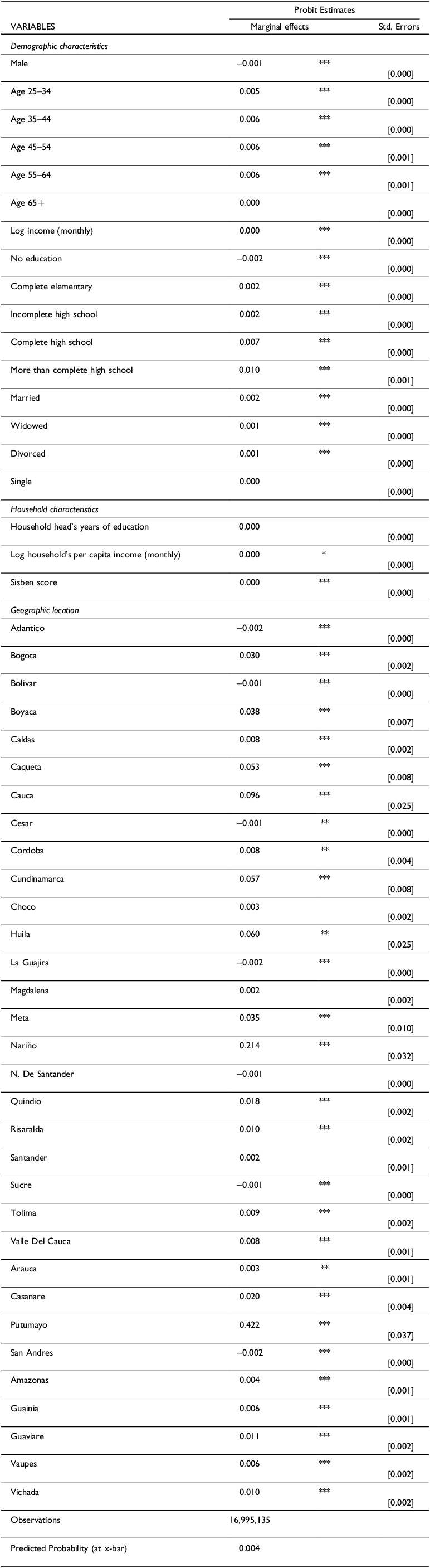
Table 6. Probability of participating in the Ponzi schemes. Results based on a probit model

***p < 0.01, **p < 0.05, p < 0.10. Standard errors are clustered at the municipal level. The dependent variable takes the value of 1 if the individual invested in the Ponzi schemes, and 0 otherwise. The dummy variable for state1 (Antioquia) is dropped to avoid collinearity. Likewise, the comparison category for marital status is Cohabitation. The omitted age category is 18–24 years, and the omitted education category is incomplete elementary education. Variables of monthly income and household per capita income are expressed in natural logarithms using the ln(1 + x) transformation. If the head of the household was not an investor but a minor in the household was, the household head is assigned the balance and capital of the minor, and hence classified as an investor. Marginal effects are calculated at the mean; for discrete variables, they represent the change from 0 to 1.

Educational attainment is positively associated with the likelihood of investing. Compared to individuals with incomplete elementary education (the omitted reference category), those with higher levels of schooling were significantly more likely to participate. In particular, the probability of investing is 0.7 percentage points higher for individuals with completed high school and 1.0 percentage points higher for those with education beyond high school. While these levels may appear modest in absolute terms, recall that “only” about 1.4% of individuals in our SISBEN sample invested in the schemes. Conversely, individuals with no formal education are significantly less likely to invest, with a marginal effect of –0.2 percentage points. Taken together, the estimates suggest a non-linear relationship between education and participation, where the effect intensifies with higher educational levels. One might reasonably expect more educated individuals to be less susceptible to investing in pyramid schemes. However, our findings suggest otherwise. A possible explanation is that these individuals believed they could strategically benefit from the schemes by exiting before their collapse. Indeed, as shown in previous sections, more educated investors were relatively more likely to be classified as winners. Nevertheless, in absolute terms, the majority – regardless of educational attainment – ultimately incurred losses.

The relationship between age and the probability of investing also exhibits a non-linear pattern. Relative to the youngest group (ages 18–24, the reference category), individuals aged 25–64 were significantly more likely to invest. On the other hand, the effect for individuals aged 65 and over is statistically zero: they are as likely to invest in the scams as their younger counterparts aged 18–24, everything else equal.

In line with the descriptive evidence, the probit estimates show that being male is associated with a lower probability of investing, though the effect is relatively small in absolute terms (–0.1 percentage points). This result confirms earlier descriptive findings and resonates with literature suggesting that women may be more susceptible to informal or high-risk financial products in the absence of strong formal financial inclusion.

Finally, there is substantial heterogeneity in participation across Colombian departments, even after controlling for individual-level covariates. The marginal effect of living in Putumayo – where DMG originated – is especially large (+42.2 percentage points), dwarfing all other regional effects. Other departments with strong positive effects include Nariño (+21.4 p.p.) and Huila (+6.0 p.p.), all regions with significant investor concentrations documented earlier. These estimates suggest that geographic proximity to the schemes’ operational centers – and possibly the strength of informal networks or word-of-mouth diffusion – played a major role in determining whether individuals invested.

Taken together, these results suggest that while individual characteristics such as education, age, and income do influence the likelihood of investing, their marginal contributions are modest relative to the large effects associated with geographical location. The magnitude of the estimated state fixed effects – particularly in departments such as Putumayo and Nariño – indicates that where individuals lived was by far the strongest predictor of participation.

7. The intensive margin: deposits, profits, and losses

Thus far, our analysis has focused on the extensive margins of participation and profitability – namely, who chose to invest and who ultimately profited. However, the size of deposits and subsequent profits and losses varies substantially across individuals, and this variation may reveal further insights about the underlying mechanisms driving investor behavior and outcomes. In this section, we examine how the magnitude of the total deposits and final balances – defined as the net position of the investor at the time of the shutdown – is associated with individual and household characteristics. While the latter reflects a combination of deposit size, withdrawal behavior, and the timing of entry and exit, its relationship with background characteristics may help clarify whether certain groups systematically gained or lost more, beyond the binary outcome of profiting or not.

To investigate these relationships, we estimate linear regression models in which the dependent variable, $ {BAL}_{i}$ , is the ratio of investor’s $ i$ final net balance relative to their deposits (i.e., the total amount invested in the schemes). We reverse the sign of the net balance variable so that positive values correspond to profits and negative values to losses. This allows regression coefficients to be interpreted in the standard direction: positive values indicate factors associated with higher relative gains (or smaller relative losses). As in previous sections, we control for a range of individual and household-level socioeconomic characteristics, as well as a full set of geographic fixed effects. We estimate the model in Equation 3 via ordinary least squares:

(3) $$ {{\mathrm{B}\mathrm{A}\mathrm{L}}_{\mathrm{i}}=\gamma {\mathrm{X}}_{\mathrm{i}}+{\mathrm{F}}_{\mathrm{s}}+{\mathrm{\varepsilon }}_{\mathrm{i}}}$$

where $ {X}_{i}$ denotes a set of individual and household-level socioeconomic characteristics, $ {F}_{s}$ is a set of state (departamento) fixed effects, and $ {\varepsilon }_{i}$ the error term. Table 7 presents the coefficient estimates and standard errors clustered at the municipal level. We present three regression models: the first utilizes the full sample,Footnote ¹⁰ while the subsequent models exclude outliers by trimming the right tail of the distribution of $ {BAL}_{i}$ as some investors exhibit extremely high balance values. Summary statistics for $ {BAL}_{i}$ are provided in Table 8.

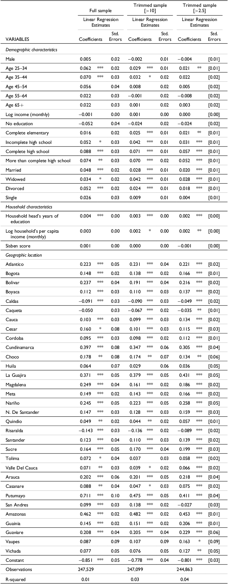
Table 7. Investors’ final balances. Results based on a linear regression model and trimmed samples

***p < 0.01, **p < 0.05, *p < 0.1. Standard errors are clustered at the municipal level. The dependent variable is the ratio of the investor’s final net balance relative to their deposits. A positive balance indicates the investor made a profit. The dummy variable for state1 (Antioquia) is dropped to avoid collinearity. Likewise, the comparison category for marital status is Cohabitation. The omitted age category is 18–24 years, and the omitted education category is incomplete elementary education. Variables of monthly income and household per capita income are expressed in natural logarithms using the ln(1 + x) transformation. If the head of the household was not an investor but a minor in the household was, the household head is assigned the balance and capital of the minor. The trimmed samples discard observations if the balance is 2.5 times or 10 times larger than the investment.

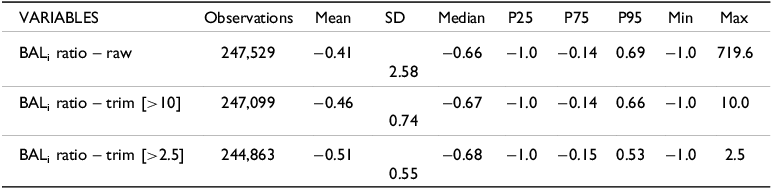
Table 8. Summary statistics, ratio of net balance to total deposits. Raw and trimmed samples

We begin by examining the role of education. Consistent with the findings on profitability and participation, we observe a positive association between educational attainment and the relative gains investors achieved. Compared to individuals with incomplete elementary education, those who completed high school earned net returns relative to their deposits that were, on average across regression models, 7.2 percentage points higher. Similarly, individuals with education beyond high school earned returns that were, on average, 6.5 percentage points higher. These effects are both statistically and economically significant and align closely with the evidence presented in earlier sections. Importantly, lower levels of attainment, such as completing elementary or attending but not finishing high school, are associated with smaller or statistically insignificant differences in returns. This mirrors the pattern observed in our probit models of participation and profitability, where the largest marginal effects were concentrated among individuals with complete secondary education or higher.

Household-level educational attainment also contributes meaningfully. Each additional year of schooling of the household head is associated with a 0.3 percentage point average increase in the investor’s return relative to deposits.

Taken together, these findings suggest that education may only begin to yield substantial financial returns – on both the extensive and intensive margins – once a critical threshold is reached, likely corresponding to the acquisition of key cognitive or numeracy skills. This interpretation is consistent with the broader financial literacy literature and recent evidence from Colombia, which documents a strong correlation between educational attainment and financial capability.

We next explore the role of age. Relative to the youngest group (age 18–24, the omitted category), investors aged 25–34 earned the highest returns, with average balance-to-deposit ratios 3.7 percentage points higher than the baseline group, averaging across regressions. The figure is similar for those aged 35–44, but without statistical significance in one of the cases. These effects align with earlier findings showing that these same age groups were more likely to participate in the schemes and had a higher probability of making a profit. In contrast, returns for older investors (45 and above) are statistically indistinguishable from those of the youngest group. This suggests a hump-shaped lifecycle pattern in financial outcomes, where middle-aged investors – likely at the peak of their earning potential and financial decision-making capacity – fared best. These patterns are consistent with existing evidence on age and financial behavior, and they echo concerns in the financial education literature about heightened vulnerability among older populations.

Turning to socioeconomic characteristics, we find that the estimated effects of being male, individual income, and the SISBEN score are all statistically insignificant. Notably, the association with household per capita income becomes statistically significant once we exclude outliers. However, this stands in contrast to the patterns observed in participation and profitability, where gender and income-related variables played a more pronounced role.

As in earlier sections, the results reveal substantial heterogeneity across departments in the relative financial outcomes of investors. Notably, Putumayo (+53 p.p. on average, across models) and Nariño (+24 p.p. on average, across models) again stand out with some of the largest effects on returns, averaging across the three estimates. These patterns reinforce the interpretation that early exposure and proximity to the scheme’s origin may have allowed certain investors to time their entry and exit more effectively, not only in terms of the extensive but also the intensive margins.