Introduction

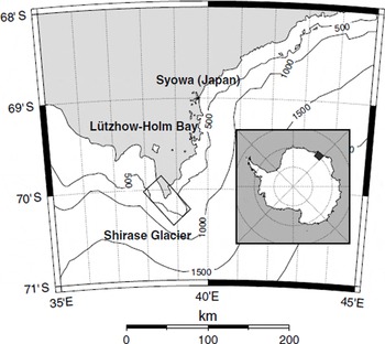
The East Antarctic ice sheet (EAIS) is primarily drained by large outlet glaciers, which play a decisive role in the dynamic behaviour of the ice sheet. Shirase Glacier is such a glacier, situated along the coast of east Dronning Maud Land (Fig. 1). Characterized by a surface velocity of up to 2700 m a⁻¹ at the calving front, Shirase Glacier is one of the fastest outlet glaciers draining the EAIS. Its mass output is estimated to be 12.5 Gt a⁻¹ at the calving front (Reference FujiiFujii, 1981). It lies in a narrow trough < 10 km in width, and which reaches depths of > 1500 m near the present calving front (Reference Moriwaki and YoshidaMoriwaki and Yoshida, 1983). In the grounded area, ice flow is strongly convergent, with 90% of the ice from the Shirase drainage basin being drained by Shirase Glacier (Reference FujiiFujii, 1981). Shirase Glacier does not calve directly into sea but ends in a 40 km long floating ice tongue, which is confined by the surrounding slow- moving ice sheet and a few nunataks.

Fig. 1.

Map of Lützow-Holm Bay, Dronning Maud Land, East Antarctica. The small rectangle corresponds to the Shirase Glacier study area as depicted in Figures 2–4.

Not much is known on the dynamics of Shirase Glacier, as difficult access hampers fieldwork activities in the downstream area of the drainage basin. The only adjacent area that has been thoroughly investigated is situated near Mizuho Plateau, roughly 200 km upstream of the grounding line. Field measurements there revealed that the ice sheet in this area is thinning at a rate of 0.5–1.0 m a⁻¹ (Reference Mae and NaruseMae and Naruse, 1978; Reference Nishio, Mae, Ohmae, Takahashi, Nakawo and KawadaNishio and others, 1989; Reference Toh, Shibuya, Yoshida, Kaminuma and ShiraishiToh and Shibuya, 1992). This thinning is believed to be the result of increasing basal sliding over time (Reference MaeMae, 1979). An analysis of European Remote-sensing Satellite (ERS) altimeter data for the period 1992–96 (Reference Wingham, Ridout, Scharroo, Arthern and ShumWingham and others, 1998) suggests a rather moderate thinning in Shirase drainage basin. Large data gaps in the downstream area, which are due to tape-recorder limitations, prevented a more accurate assessment of the imbalance in this region. Besides Mizuho Plateau, the calving front of Shirase Glacier has been the subject of a number of investigations, mainly through analysis of aerial photographs (Reference Nakawo, Ageta and YoshimuraNakawo and others, 1978; Reference FujiiFujii, 1981).

The position of the calving-front area of Shirase Glacier is depicted in Figure 2. In this area the floating ice tongue disintegrates into a conglomerate of several large icebergs, which are clearly visible in this satellite image. These icebergs stick together in the fast ice that covers the entrance of Lützow-Holm Bay, forming a continuation of the tongue. At regular intervals (few to tens of years), these icebergs are cleared from the area as the fast ice breaks up in Lützow– Holm Bay. This repeated change is also visible from an analysis of 1963 U.S. Department of Defense declassified intelligence satellite photography (DISP), Landsat data and RADARSAT-1 image mosaics (Reference Kim, Jezek and SohnKim and others, 2001). In 1962 this iceberg conglomerate was at its furthest extent. It then retreated about 60 km in the mid-1970s to a position that nearly matched its position in 2000. Between 1997 and 2000 a retreat of about 12 km was observed (personal communication from K. C. Jezek, 2001). It should be stressed, however, that such retreat is not a retreat of the grounding line of the glacier, nor of its calving front, but a removal of icebergs that have already calved off.

Fig. 2.

Amplitude image of the ERS-1 scene of Shirase Glacier acquired on 2 June 1996. Ice flow is primarily from the bottom of the image towards the top. The x axis corresponds to the satellite look direction (slant range), while the y axis corresponds to the direction of satellite’s motion (azimuth). CF, calving front; FT, floating tongue; GL, grounding line; A, Shirase Glacier main stream; B, secondary stream.

This paper presents insight into the present-day dynamics of Shirase Glacier, based on a satellite-derived surface velocity field of the area near the grounding line. Surface displacements are determined from ERS synthetic aperture radar (SAR) imagery by speckle tracking using phase correlation. A large-scale force budget is then applied to estimate the major forces balancing the driving stress. Finally, the present dynamical state of Shirase Glacier is estimated by analyzing its mass budget.

Interferometric Processing

Interferometric processing of SAR imagery allows for determination of the surface displacement field with a centimeter-level precision. Two co-registered SAR images are used to generate an interferogram, which is a plot of phase shifts as a function of position. The phase in the resulting interferogram can be divided into two parts. The first part, the interferometric phase, contains relative optical-path variations over the time interval between the two image acquisitions. The second part, the coherence term, contains phase differences due to changes in the response of illuminated scatterers. Optical-path variations have different origins: (i) an orbital phase depending on the viewing geometry of the SAR image pair, (ii) a topographic phase due to the relief of the imaged area, and (iii) a differential phase caused by local displacements of the ground surface in consecutively scanned images. Of interest here is the differential phase Δφ _d, a measure of the displacement of a ground surface point in the look direction of the spacecraft, within the time-span between the acquisition of the two images, i.e. Δφ _d = (4π/λ) Δz, where λ = 5.6 cm is the wavelength of the ERS radar and Δz is the look-direction component of the optical-path variation. Half a wavelength of displacement in the look direction produces a phase shift of 360°. If the displacement has a component in the direction of the satellite’s motionFootnote ¹ , it has no influence on the differential phase. The altitude of ambiguity is a measure for the sensitivity of an interferometric pair to topography, which depends on the perpendicular baseline, wavelength and radar look angle. The altitude of ambiguity is typically of the order of 100 m for most interferometric applications using ERS sensors. Sensitivity to displacement (or to any other local optical-path variation) depends on the wavelength of the radar.

Retrieval of ERS SAR images from Antarctica is difficult. Because of the satellite orbital configuration, only the area north of 78° S can be imaged. Moreover, only a fraction of the potential imagery may be retrieved, depending on operating procedures and proximity to receiving stations. For the purpose of this study, only three suitable ERS-1/-2 tandem pairsFootnote ² were acquired at Syowa station, Antarctica. Among these three pairs, the pair of 2 and 3 June 1996 has a favorable altitude of ambiguity with respect to differential interferometry (i.e. near-zero baseline). The resulting interferogram is nearly insensitive to topography. For this pair of SAR images, however, glacier movement is primarily perpendicular to the satellite look direction, to which differential interferometry is not sensitive. Horizontal ice displacement was therefore obtained by means of speckle tracking using phase correlation (Reference DerauwDerauw, 1999). This method uses the maximum interferometric coherence to match small image kernels (windows) from two co-registered SAR images of the same region. The technique is comparable to speckle tracking (Reference Gray, Mattar, Vachon and SteinGray and others, 1998; Reference Michel and RignotMichel and Rignot, 1999), but uses the phase information instead of the coherent speckle information in the amplitude images.

For a small image kernel (master) centred around a particular anchor point in one of the SAR images, a conjugate point was sought in the other image (slave) by calculating the local interferometric coherence between the master image kernel and a moving slave kernel of the same size. The maximum local coherence of all searches refers to the corresponding point, which was determined with sub-pixel accuracy. For each anchor point we obtain the relative azimuth and range displacement, the tracked coherence and the tracked interferometric phase. Based on the latter, a so-called tracked interferogram can be calculated, in which the noise induced by mis-registration is removed. In order to measure more accurately the coherence and the localization of its local maximum, the SAR scenes were oversampled by a factor 2.5 using a phase-preserving interpolation tool. A mesh of anchor points covering the whole scene with a grid spacing of 3 pixels in range and 15 pixels in azimuth was defined so that displacement measurements were obtained every 24 m in x and y. The optimal kernel sizes proved to be 25 pixels in azimuth and 5 pixels in range, after oversampling. The tracked coherence shows a much higher coherence over the surface of Shirase Glacier compared to the coherence obtained previously. The relative shifts in x and y direction, obtained with sub-pixel accuracy from speckle tracking, are then translated to surface velocities using a few ground-control points situated on non-moving parts of the scene. Baseline corrections for range offsets and geometric corrections for azimuth offsets were not applied. Errors in velocities obtained by speckle tracking using phase correlation are determined from the non-moving parts in the scene. We therefore sampled points on rock outcrops, evenly spread over the whole image. Errors in range and azimuth velocity are calculated as σ_u ≈ 74 m a⁻¹ and σ_v ≈ 57 m a⁻¹, respectively.

The technique of speckle tracking using phase correlation has the advantage that a so-called tracked interferogram can be calculated, which gives, after unwrapping, the displacement in the range direction. In theory, the accuracy of this unwrapped range velocity is very high, i.e. depending on the wavelength of the radar. The error is given by

(1)

where α = 23° is the incidence angle and λ is the wavelength of the radar. is the error estimate in phase (Reference Rodriguez and MartinRodriguez and Martin, 1992; Reference Just and BamlerJust and Bamler, 1994), where γ is the coherence and N the interferometric multi-looking factor, i.e. the number of full-resolution samples used for the coherence estimation. For the present case, taking into account the kernel size and the zoom factor, N = 50. For an average coherence γ = 0.7, Equation (1) gives an error in unwrapped range velocity of . However, additional errors such as those due to atmospheric effects could well be of the order of 5 m a⁻¹ (Reference Joughin, Fahnestock and BamberJoughin and others, 2000). Furthermore, tidal displacement affects the unwrapped velocity as well. Despite the 24 hour difference between both images, tidal displacement could well be of the order of 10–15 cm in Lützow–Holm Bay (Reference Aoki, Ozawa, Doi and ShibuyaAoki and others, 2000), leading to an error of 90–130 m a⁻¹ in the unwrapped velocity field. Due to these large uncertainties the unwrapped range velocity field was not included in the analysis below.

Surface Velocities and Strain Rates

The displacements obtained from the interferometric analysis were interpolated on a regular grid of 200 by 200 m. Since this velocity field still contains high-frequency noise associated with the errors noted above, the original velocity-field velocity was smoothed by averaging over a larger window of 6 × 6 km. Smaller window sizes (1–6 km) were used as well, but did not hamper the analysis from the viewpoint of “overseeing” ice dynamics. Using such large windows has the advantage that all high-frequency noise is removed. Velocities are thus taken as the mean of all velocity estimates within the window. Velocity gradients, used to calculate strain rates, are considered constant within the area of any window and are determined through a linear regression analysis of all u and v values in that window with respect to the x and y directions (Figs 3 and 4). Since the major ice motion is in the y direction, the major strain components are the surface longitudinal strain rate , the surface transverse strain rate , and the surface lateral shear-strain rate , defined as

(2)

(3)

(4)

Fig. 3.

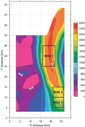
Magnitude of the surface velocity field of Shirase Glacier (m a⁻²). Large-scale force-budget calculations are carried out for the three depicted boxes.

Fig. 4.

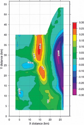
Shirase Glacier surface shear-strain rate

where the overbar denotes the averaging over the window. Velocities on the floating ice tongue are nearly constant over the entire length of the tongue. No significant acceleration along the central flowline of the ice tongue is observed. This is in contrast to the grounded area(zone A, Fig. 2), where ice speed increases from 1000 to 2000 m a⁻¹ over a distance of ≈10 km (Fig. 3). The resulting longitudinal strain rate is on the order of 0.1 a⁻¹. Previous estimates of the velocity field on Shirase Glacier were based on aerial photographs of 1962, 1969, 1975 and 1977 of the floating part of Shirase Glacier; Reference FujiiFujii (1981) calculated calving-front velocities of 2500–2700 m a⁻¹. The ERS velocities, however, are slightly lower than the photogrammetric ones, probably due to the shorter time-span over which the ERS images were evaluated, and due to the fact that the ERS images were taken in the winter period.

A map of the surface lateral shear strain rates on Shirase Glacier is given in Figure 4. High values are associated with the sides of the glacier, especially at both sides of the floating ice tongue where it is fringed by the grounded ice sheet and a few rock outcrops. Even in the grounded part of the glacier (the grounding line is denoted by GL in Figure 2) this channel effect can be noticed, as the high values of occurring at the western margin of the glacier continue upstream towards the south (Fig. 4). It can also be seen that the calving front (CF in Fig. 2) coincides with the area where the lateral shearing ends, since downstream of the calving front a mixture of sea ice and open water occurs at both sides of the “ice-tongue conglomerate”.

Large-Scale Force Budget of Shirase Glacier

The calculation of the force budget is based on a similar analysis by Reference Rolstad, Whillans, Hagen and IsakssonRolstad and others (2000), i.e. by assessing the relative importance of the forces controlling the ice flow in a large imaginary box in the glacier. We adapt these force balance calculations to three dimensions by integrating numerically over the ice thickness in order to estimate the horizontal and basal shear stresses and the basal velocity in each box. Hence, each box consists of a number of planes parallel to the surface. Three boxes of dimensions W × L (L is taken parallel to the glacier motion) were selected on the glacier surface. Box 1 is situated on the floating ice tongue, box 2 is centred on the grounding line and box 3 is inland from the grounding line (Fig. 3). Ice flow is primarily in the y direction, so only the force balance in the y direction is discussed here. For a Cartesian coordinate system the force balance yields (Reference Van der Veen and WhillansVan der Veen and Whillans, 1989)

(5)

where ∇ _S is the surface gradient, R_yz is the horizontal shear stress, R_xy the lateral shear stress, and R_yy the longitudinal resistive stress in the direction of the flow. To obtain the force budget and an estimate of the basal drag, Equation (5) has to be integrated from the base of the glacier to the surface, yielding

(6)

where τ _d = −ρgH∇s is the driving stress, and τ _b the basal drag, or the sum of all resistance to the flow at the base. Stresses are related to strain rates by means of a constitutive equation, Glen’s flow law for polycrystalline ice, with n = 3.

(7)

(8)

(9)

where is the effective strain rate, or the second invariant of the strain-rate tensor, defined by , for i, j = x, y, z, where summation over repeat indices is implied. The stiffness parameter B is related to temperature through an Arrhenius-type relation (Reference HookeHooke, 1981).

The major simplification we will make is that all measured Footnote ³ strain rates are kept constant with depth and are equal to their surface value (cf. Høydal, 1996). This assumption can be made, as the high surface velocities in this area will account for a more-or-less block-flow movement. Their associated stresses will vary with depth, as the flow-law parameter B changes with temperature and the effective strain rate is a function of the depth-varying horizontal shear-strain rate as well.

Numerical solution

Equation (5) is integrated numerically from the surface of the glacier to an arbitrary height z, starting with the surface stress field, and using 50 equidistant layers in the vertical. A stress-free surface implies that R_yz (s) = R_yy (s)∇s (Reference Van der Veen and WhillansVan der Veen and Whillans, 1989). Values of R_xy and R_yy are calculated for the sides of the box, based on the mean values of the strain rates at these sides. The horizontal shear stress at a height z in the ice box is then given by

(10)

where subscripts “up” and “down” refer to the upstream and downstream sides of the box, respectively, and subscripts “east” and “west” refer to the eastern and western sides of the box, respectively. At each level the effective strain rate is calculated, while the horizontal shear-strain rate is obtained from Equation (8). Assuming no vertical shear, the horizontal shear-strain rate is related to the velocity field by , from which the velocity at each level can be calculated. Once the integration reaches the base, the stress balance is obtained by integrating the stresses at depth over the whole ice column, leading to

(11)

To determine the flow-rate factor B, the ice temperature was kept equal to the surface temperature (using data from Reference Satow, Kikuchi and HigashiSatow and Kikuchi, 1995) for two-thirds of the ice thickness, and then increased linearly to the pressure-melting point for the bottom third. Similar temperature parameterizations are found elsewhere (e.g. Reference Mayer and HuybrechtsMayer and Huybrechts, 1999). High basal temperatures are very likely, as radio-echo soundings in this area have demonstrated that a water layer should be present in the downstream area of the grounded part of Shirase Glacier (Reference Nishio and UratsukaNishio and Uratsuka, 1991). Experiments with a linear temperature profile (linearly decreasing from surface to bottom) gave similar results for the force balance; only the determination of the basal velocity seems slightly influenced by this choice. Ice-thickness measurements are rather sparse in the downstream part of Shirase Glacier. A few measurements are obtained from airborne radio-echo sounding surveys by the Japanese Antarctic Research Expedition (Reference Wada and MaeWada and Mae, 1981; Reference Mae and YoshidaMae and Yoshida, 1987). One data point near the grounding line is listed in the BEDMAP database (H = 880 m; Reference Lythe and VaughanLythe and others, 2000).

The calculated strain rates and their associated stresses for the four sides of the boxes are given in Tables 1 and 2. Errors are determined from the theory of error propagation. For instance, the error in lateral shearing (Equation (7)) is

(12)

Table 1.

Measurements and averaged strain rates at the sides of the boxes

Table 2.

Calculated stresses and force-balance components based on measurements and calculations given in Table 1

Similar expressions are found for all other calculated variables. Despite the large errors associated with the uncertainties in input parameters, such as glacier geometry and velocity, the propagated errors in the force-budget calculations are significantly smaller than the values themselves, so that some trends can be discerned (Table 2). In the floating tongue (box 1), the basal drag should be zero by definition, which is confirmed by the numerical calculations. Lateral drag is more important than the driving stress, but the longitudinal stress gradient cannot be neglected in enhancing the ice flow. The impact of horizontal shear is negligible, as the basal velocity equals the surface value. Horizontal shear strain rates are zero over the whole ice thickness (Fig. 5), and the stress components R_xy and R_xx vary according to the assumed temperature profile (Fig. 6).

Fig. 5.

Shear strain rate as a function of depth for box 1 (•), box 2(○) and box 3 (Δ).

Fig. 6.

Scaled longitudinal resistive stress as a function of depthfor box 1 (•), box 2 (○) and box 3 (Δ). The variation of the scaled R_xy with depth is similar to this graph, and therefore not shown.

Near the grounding line (box 2), driving stresses are large (>300 kPa), due to steep surface and relatively thick ice. The basal drag is less than the driving stress, primarily because of the resistance provided by lateral drag and the longitudinal stress gradient. Although ice speed increases in the direction of the flow, the acceleration is different in the grounded and the floating part. In the grounded part, ice acceleration is important, while in the floating ice tongue is much smaller (but still positive) due to important shearing at the margins. This reduction in ice acceleration leads to a negative longitudinal stress gradient , which is most pronounced at the grounding line (box 2). This means that longitudinal stress gradients act to resist the driving stress at the grounding line. Normally, one would expect them to be “pulling” in the downstream direction, i.e. an acceleration once the glacier becomes afloat. The “pushing” seems thus due to an important (lateral) shearing at the sides of the floating part of the glacier.

Horizontal shear is the most important stress component in the force budget of boxes 2 and 3. Shear-strain rates at depth exceed 0.8 a⁻¹, which is far more important than lateral shear and normal strain rates (Fig. 5). Consequently, the depth variation of the resistive stresses R_xy and R_yy is non-linear and depends not only on temperature variations but on the impact of high horizontal shear-strain rates as well (Fig. 6). It is clear that depth-averaged solutions cannot be used and the numerical integration is in order here. Although horizontal shear is dominant in this area, the impact of the deformation velocity u _d in the total velocity field is very low, i.e. 5.5% and 8.1% for box 2 and box 3, respectively, which means that more than 90% of the vertical mean horizontal velocity is due to basal sliding.

In short, the above force-budget calculations demonstrate that, despite the high surface and basal velocities, Shirase Glacier is distinguished from a typical West Antarctic ice stream, such as Whillans Ice Stream, by the relative importance of driving stress and basal drag, even though basal drag is to some extent reduced by the impact of lateral drag — due to the convergent flow upstream of the grounding line — and the longitudinal stress gradient. The latter is only of importance in a small zone centred around the grounding line.

Large-Scale Mass Budget of Shirase Glacier

To determine the mass budget of Shirase Glacier, we compare the ice flux at the grounding line with balance-flux calculations of the Antarctic ice sheet. Based on an update of the Reference Giovinetto and BentleyGiovinetto and Bentley (1985) dataset of the surface mass balance, and the refined surface-elevation dataset of Reference Bamber and BindschadlerBamber and Bindschadler (1997), Reference Huybrechts, Steinhage, Wilhelms and BamberHuybrechts and others (2000) calculated balance fluxes of the Antarctic ice sheet on a 20 km grid. The balance flux at a certain position in the ice sheet equals the total amount of accumulated ice (the surface integral of the surface mass balance) that is drained in the direction of the flow towards that position. Reference Huybrechts, Steinhage, Wilhelms and BamberHuybrechts and others (2000) thus find a total mass flux at the gate of Shirase Glacier (which, because of the resolution, represents the discharge through both streams A and B in Figure 2) of 12.4 Gt a⁻¹. Since approximately 82% of the total ice discharge in Shirase Glacier is through stream A (Reference FujiiFujii, 1981), the balance fluxes of Reference Huybrechts, Steinhage, Wilhelms and BamberHuybrechts and others (2000) account for a mass flux of 10.2 Gt a⁻¹ at the grounding line of Shirase Glacier (GL in Fig. 2). The accuracy of the balance-flux estimates depends on the accuracy of the accumulation data, the surface elevation data, the distance over which the surface gradients are calculated and the grid resolution. This leads to an error of 10–20%, the latter being a worst-case estimate, or 1.0–2.0 Gt a⁻¹.

From the present study, the mass flux at the grounding line can also be determined, albeit limited to stream A. For a vertical mean horizontal velocity of 2035 ± 74 m a⁻¹ (a value determined from the force-budget integration), a mean ice thickness of 900 ± 100 m and a cross-sectional width of 8.3 km, we obtain a mass flux of 13.8 ± 1.6 Gt a⁻¹ at the grounding line. These calculations lead to a mass deficit (negative imbalance) of 3.6 ± (2.6 − 3.6) Gt a⁻¹. The large errors in the mass-budget calculations show that a slight negative imbalance might exist, but the situation is likely close to equilibrium conditions. The inferred imbalance, spread out over the whole drainage basin, would lead to a thinning rate of 0–4 cm a⁻¹. This value is much lower than the 0.5–1.0 m a⁻¹ suggested by other authors (e.g. Reference Mae and NaruseMae and Naruse, 1978; Reference Nishio, Mae, Ohmae, Takahashi, Nakawo and KawadaNishio and others, 1989; Reference Toh, Shibuya, Yoshida, Kaminuma and ShiraishiToh and Shibuya, 1992). Even if we limit the thinning to the area of Mizuho Plateau, i.e. the area below the 2400 m contour, the thinning rate would be of the order of 0–17 cm a⁻¹, still an order of magnitude lower than suggested by field evidence in the downstream area of Shirase drainage basin.

Discussion and Conclusions

In this paper, the surface velocity field of Shirase Glacier, a fast-flowing East Antarctic outlet glacier, is inferred from ERS SAR images by means of speckle tracking using phase correlation. Surface strain rates were calculated based on these velocity estimates. A large-scale vertically integrated force budget then allowed for the determination of the major stress components (basal drag, lateral drag and the longitudinal stress gradient opposing the driving stress) in the floating ice tongue, near the grounding line and on the inland slope. Results showed that for the grounded glacier system, basal drag is the most important stress component resisting the driving stress (80–87% of the driving stress). Lateral drag accounts for <15% of the driving stress. Longitudinal stress gradients, however, have a limited effect and are confined to a small area a few kilometers in length near the grounding line, even though longitudinal stresses are dominant over the whole grounding zone and inland slope region. Moreover, longitudinal stress gradients resist the driving stress at the grounding line (“pushing”), while they enhance the flow in the floating part (“pulling’’).

Such a situation is in contrast with the ice-dynamic conditions in the transition zone between an ice sheet and an ice shelf, where not only do longitudinal stress gradients have a limited effect, but also longitudinal stress, lateral shear and basal sliding are unimportant (Reference Mayer and HuybrechtsMayer and Huybrechts, 1999) . Despite high basal velocities (>90% of the total velocity is due to basal sliding), Shirase Glacier is also clearly distinguished from an ice stream by a large driving stress and basal drag in the grounded part of the transition zone.

A comparison with a balance-flux distribution of the Antarctic ice sheet (Reference Huybrechts, Steinhage, Wilhelms and BamberHuybrechts and others, 2000) shows that the downstream area of Shirase Glacier is more or less in equilibrium, although a slight mass deficit (thinning) might exist. This thinning seems of lesser magnitude than suggested in previous studies and measurements in the downstream area of Shirase drainage basin (Reference Mae and NaruseMae and Naruse, 1978; Reference Nishio, Mae, Ohmae, Takahashi, Nakawo and KawadaNishio and others, 1989; Reference Toh, Shibuya, Yoshida, Kaminuma and ShiraishiToh and Shibuya, 1992).