


Introduction
The relationship between energy and agricultural commodity markets has garnered significant attention over the past two decades, particularly in light of increased food price volatility and mounting global energy concerns. Following the 2008 financial crisis, agricultural prices have exhibited heightened fluctuations, with multiple channels – macroeconomic instability, speculative activity, exchange rate dynamics, and structural changes in food production – contributing to this volatility. Among these, energy markets, particularly oil and natural gas, play a central role by affecting agriculture both as a direct input and through their influence on intermediate goods such as fertilizers.
Modern agricultural systems have become increasingly industrialized and energy-intensive. Energy is required not only for mechanized farming and transportation but also in the production of synthetic fertilizers and pesticides. Crude oil affects the cost of transportation, irrigation, and machinery, while natural gas is a key input in fertilizer production, especially urea. Consequently, understanding how fluctuations in energy prices propagate through these channels to affect agricultural commodity prices is essential for both economic analysis and policy formulation.
While existing literature has extensively examined price and volatility spillovers between energy and agricultural commodities, results remain inconclusive. Some studies suggest positive co-movements, while others find negligible or even negative effects. These inconsistencies may stem from model specifications, data frequency, or the neglect of underlying nonlinear dynamics and indirect transmission channels, such as the role of fertilizers.
This paper seeks to contribute to this literature by disentangling the direct and indirect effects of energy prices on major agricultural commodities – namely wheat, maize, and soybeans. We distinguish two key transmission channels: (i) the direct effect of crude oil on commodity prices as a production and transportation cost, and (ii) the indirect effect via fertilizers, where crude oil and natural gas prices influence the cost of Di-Ammonium Phosphate (DAP) and Urea fertilizers, which in turn affect crop prices.
To model these relationships, we employ an empirical strategy that incorporates conditional covariances extracted from a BEKK-GARCH model – applied to energy and fertilizer prices – to capture time-varying volatility and interactions among these series. These covariances, along with crude oil, natural gas, DAP, and Urea prices, are then used in a dynamic specification of crop prices. We control for potential non-stationarity and cyclical dynamics in the data through the Flexible Fourier Form approach, which allows for smooth, nonlinear trends without imposing restrictive structural break assumptions. We should also note that the estimation sample is restricted to the period before the Russian–Ukrainian war to avoid contamination from this highly idiosyncratic shock, which severely disrupted the global grain value chain through export blockades, input price spikes, and unprecedented policy responses – dynamics that are unlikely to reflect broader structural relationships.
Our findings indicate that both direct and indirect energy price channels significantly impact agricultural commodity prices. In particular, crude oil prices exert an immediate and significant effect on all three grains, while fertilizer prices show lagged and heterogeneous effects. The conditional covariances extracted from the BEKK-GARCH model are also statistically significant, particularly during periods of market turbulence, highlighting the importance of co-movements between energy and fertilizer markets.
The rest of the paper is organized as follows. Section Literature review describes the data sources and econometric methodology. Section Data and methodology presents the empirical results. Section Results discusses the findings and offers concluding remarks.
Literature review
The linkage between energy and agricultural commodity markets has been extensively studied, especially in the aftermath of the 2007–2008 food and energy price spikes. Numerous studies attribute rising food prices to macroeconomic uncertainty, supply-demand imbalances, exchange rate volatility, biofuel policies, and increased speculative activity (Avalos 2014; Headey and Fan Reference Headey and Fan2008; Yuan et al. Reference Yuan, Tang, Wong and Sriboonchitta2020). Among these drivers, energy prices – particularly oil and natural gas – have received significant attention due to their central role in modern agriculture.
Energy affects agriculture through both direct and indirect channels. The direct channel encompasses input costs related to mechanization, irrigation, transportation, and processing. The indirect channel operates through the energy-dependance of key agricultural inputs, notably synthetic fertilizers and pesticides (Aye and Odhiambo Reference Aye and Odhiambo2021; Woods et al. 2010). Oil prices, for example, influence fuel and logistics costs, while natural gas serves as a primary feedstock for nitrogen-based fertilizers such as Urea (Pimentel and Pimentel Reference Pimentel and Pimentel2008).
Although this dual channel is theoretically well established, empirical studies have yielded mixed results. Some studies report weak or neutral relationships between crude oil and agricultural commodity prices (Nazlioglu Reference Nazlioglu2011; Yu et al. Reference Yu, Wang and Lai2008; Zhang et al. Reference Zhang, Lohr, Escalante and Wetzstein2010), while others find positive and significant co-movements (Avalos and Lombardi Reference Avalos and Lombardi2015; Chen et al. Reference Chen, Kuo and Chen2010; Jadidzadeh and Serletis Reference Jadidzadeh and Serletis2018; Sun et al. Reference Sun, Mirza, Qadeer and Hsueh2021). Still others suggest asymmetric spillovers or structural breaks associated with financialization and speculative behavior (Al-Maadid et al. Reference Al-Maadid, Caporale, Spagnolo and Spagnolo2017; Bonato and Taschini Reference Bonato and Taschini2016).
Fertilizers represent a critical yet underexplored component in the transmission of energy prices to agricultural commodity prices. Nitrogen (N), phosphorus (P), and potassium (K) fertilizers are essential for yield growth and are highly energy-intensive to produce. Di-Ammonium Phosphate (DAP), widely used in cereal production, relies heavily on oil-based inputs for transportation and processing. Urea, the most commonly used nitrogen fertilizer globally, is synthesized from ammonia – derived primarily from natural gas (Ding et al. Reference Ding, Ye, Fu, He, Wu, Zhang, Zhong, Kung and Fan2023; Heffer and Prud’homme Reference Heffer and Prud’homme2016). Wongpiyabovorn and Hart (Reference Wongpiyabovorn and Hart2024) conduct an ARDL analysis to examine the pass-through relationship between natural gas and corn prices on nitrogen fertilizer prices in the U.S., taking into account the biofuel mandates, improvements in shale gas extraction after 2009 and the strong dependance of corn production on fertilizer costs. Even though their study is limited to the US, they claim that the global natural gas shocks have emerged as a factor affecting fertilizer prices.
Studies highlight the global importance of fertilizers in supporting grain output and stabilizing productivity (Aghabeygi et al. Reference Aghabeygi, Louhichi and Gotor y Paloma2022; McArthur and McCord Reference McArthur and McCord2017). Increases in global fertilizer prices – driven in part by energy markets – can thus have significant delayed effects on crop markets. Despite this, the empirical literature often treats fertilizer prices as exogenous or omits them entirely from price transmission models.
A recurring limitation in the literature is the reliance on linear models or symmetric volatility frameworks that may overlook nonlinearities and evolving price dynamics. Moreover, few studies explicitly separate direct energy effects from indirect fertilizer-driven effects. The joint behavior of energy and fertilizer prices – especially their conditional covariances – has received limited attention despite its potential importance during times of global market stress.
This study addresses these gaps by modeling both direct and indirect linkages from energy to agriculture, employing conditional covariances extracted from BEKK-GARCH models, and controlling for non-linearities via the Flexible Fourier Form. To our knowledge, this approach is novel in the context of energy-agriculture price dynamics and offers a more nuanced view of co-movement and volatility spillover effects.
Data and methodology
This study employs monthly data spanning the period from February 1991 to February 2021 to investigate the direct and indirect effects of energy prices on agricultural commodity prices. To ensure completeness and reflect recent market developments, the dataset has also been extended to cover the period up to December 2024, following the same methodological framework. The extended results, presented in the Appendix, allow for an updated comparison while maintaining the original sample as the primary focus of analysis, given its coverage of a relatively stable pre-war period that ensures methodological consistency and comparability. The focus is on three major grains – wheat, maize, and soybeans – due to their global production and trade significance (Erenstein et al. Reference Erenstein, Chamberlin and Sonder2021; Szerb et al. Reference Szerb, Csonka and Fertő2022). Crude oil and natural gas prices serve as proxies for energy inputs, while Di-Ammonium Phosphate (DAP) and Urea represent fertilizer inputs.
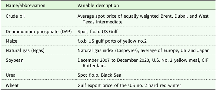
Crude oil is used as a benchmark for energy, represented by the average spot price of Brent, Dubai, and West Texas Intermediate. Natural gas is captured via a Laspeyres index averaging prices across Europe, the U.S., and Japan. The agricultural commodity prices are based on trade-relevant benchmarks: U.S. No. 2 yellow corn (f.o.b. Gulf ports), U.S. No. 2 hard red winter wheat (Gulf export), and U.S. No. 2 yellow soybean meal (CIF Rotterdam). Fertilizer prices are represented by DAP (spot, f.o.b. U.S. Gulf) and Urea (spot, f.o.b. Black Sea).
All price data are sourced from the World Bank’s Commodity Price Data – “Pink Sheet” (World Bank 2023). Table 1 presents an overview of variable definitions and sources.
Variable names, and descriptions

Source: World Bank.
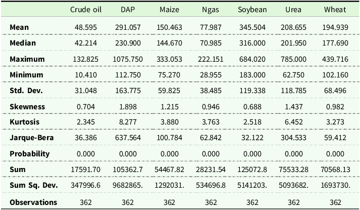
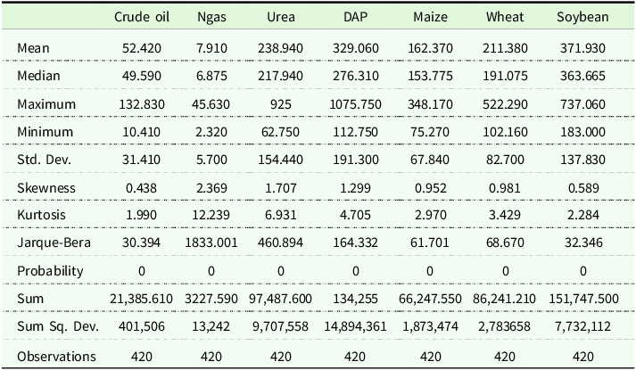
The descriptive statistics of the variables are presented in Table 2. There are 362 observations for each variable. Between February 1991 and February 2021, the Crude Oil price varied between 10.4 and 132.8, with a mean and standard deviation of 48.5 and 31.8. Ngas price varied between 28.9 and 222.1, with a mean and standard deviation of 77.9 and 38.4. Among fertilizer items, Urea and DAP show dramatic price movement from 62.7 to 785, 112.7 to 1075.7 respectively, with a mean and standard deviation of 208.6 and 118.7, 291 and 163.7 respectively. Maize, wheat, and soybean prices also fluctuated significantly in the sample period, ranging from 75.2 to 333, 102.1 to 439.7, and 75.2 to 333 respectively. Soybean has the highest mean value and DAP has the highest standard deviation. According to JB statistics, it is evident that all price series exhibit a non-normal distribution.
Descriptive statistics

Source: Authors calculation.
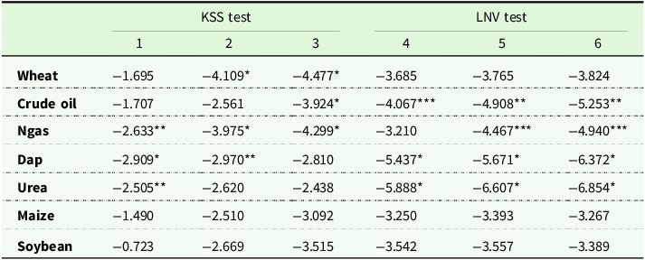
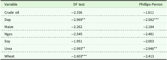
When beginning the analysis, standard unit root tests are used to examine the stochastic properties of the variables. As seen in Table 3, only fertilizer series (Dap and Urea) are I(0), but others are I(1). Therefore, there is a unit root problem in most of the series.
Unit root test results
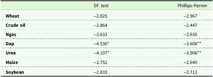
Notes: *1% and **5%.
Critical values for Dickey-Fuller and Philips-Perron are −3.983, −3.422, −3.134 (1%,5%,10% respectively).
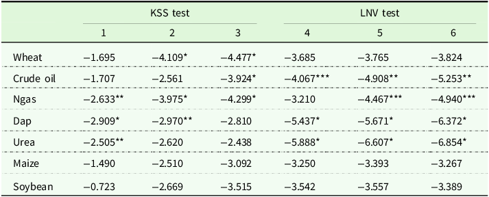
Since, in traditional tests, the null hypothesis is one of the unit-root linearity, for the identification of the nonlinear structure (state-dependent or time-dependent) of the variables, a battery of tests (Leybourne, Newbold, and Vougas (LNV), Reference Leybourne, Newbold and Vougas1998 and Kapetanios, Shin and Shell (KSS), Reference Kapetanios, Shin and Snell2003) is employed to see whether each variable is governed by a stationary process with different nonlinear structures. As seen in Table 4, LNV model-b is the most suited one, but still wheat, maize, and soybean series are insignificant.
Unit root test results

Notes: *1%, **5% and ***10%.
1-raw data; 2-De-meaned; 3-De-meaned and de-trended; 4-Lnv Model-a; 5-Lnv Model-b; 6-Lnv Model-c.
Critical values for KSS – raw data −2.82, −2.22, −1.92; De-meaned, −3.48, −2.93, −2.66; De-trended, −3.93, −3.40,−3.13 (1%,5%,10% respectively).
Critical values for LNV – Model a, −4.88,−4.23,−3.91; Model b, −5.48, −4.77, −4.43; Model c, −5.65, −5.01, −4.70 (1%,5%,10% respectively).
According to Becker et al. (Reference Becker, Enders and Lee2006), employing a Fourier function allows smooth changes when performing a unit root test. The Fourier approach’s fundamental benefit is its capacity to accurately model the behavior of deterministic functions of unknown form, even when the function is not periodic in nature. Therefore, it is not necessary to define the location, kind, or quantity of breaks. The Flexible Fourier Form allows for greater flexibility in modeling periodic components, therefore models based on the Flexible Fourier Form may provide more accurate forecasts especially when the data have nonlinear patterns (Enders and Lee Reference Enders and Lee2012). In order to do this, the Flexible Fourier Form and DF type Unit Root test (FFF), as recommended by Enders and Lee (Reference Enders and Lee2012), is used.
The following Equation is estimated to compute the FFF test statistic:
 $${\rm{\Delta }}{y_t} = \alpha + \beta t + \mu {y_{t - 1}} + {\delta _{1k}}\sin \left( {2\pi kt/T} \right) + {\delta _{2k}}\cos \left( {2\pi kt/T} \right) + {e_t}$$
In Equation (1), π = 3.1416, t, T, and k indicate the trend term, sample size, and a particular frequency. To determine the optimal value of frequency, k*, Equation (1) is estimated for the values of k, and the value that produces the minimum residual sum of squares (RSS) is chosen.
As seen in Table 5, all variables in question are stationary.
Enders and Lee (Reference Enders and Lee2012) Flexible Fourier Form and DF type unit root test results

Notes: *1% and **5%.
(Critical values for FFF – constant), −4.62, −4.01, −3.69(1%, 5%, 10% respectively for k = 2); −4.38, −3.77, −3.43(1%, 5%, 10% respectively for k = 3); Constant, trend −3.93, −3.26, −2.92(1%, 5%, 10% respectively for k = 2); –3.74, −3.06, −2.72(1%, 5%, 10% respectively for k = 3).
Since the assumption of stationarity is generally satisfied, to pretest for a nonlinear trend, Becker et al. (Reference Becker, Enders and Lee2006) followed to test the null hypothesis of linearity against the alternative of a nonlinear trend with a given frequency k. Enders and Lee (Reference Enders and Lee2012) propose the use of the following F-statistic:
 $$F\left( k \right) = {{\left( {SS{R_0} - SS{R_1}\left( k \right)} \right)/2} \over {SS{R_1}\left( k \right)/(T - q)}}$$
where $SS{R_1}\left( k \right)$
denotes the sum of squared residuals (SSR) when Fourier transforms enter the equation, q is the number of regressors, and
$SS{R_1}\left( k \right)$
denotes the sum of squared residuals (SSR) when Fourier transforms enter the equation, q is the number of regressors, and $SS{R_0}$
denotes the SSR from the regression without the trigonometric terms. In all cases, the null is rejected in favor of a nonlinear trend, given the frequency k.
$SS{R_0}$
denotes the SSR from the regression without the trigonometric terms. In all cases, the null is rejected in favor of a nonlinear trend, given the frequency k.
From the FFF unit root test result, we see that all series have stationarity features. The process is stationary after employing the detrending. It should be noted that the main contribution of the nonlinear trend is the elimination of the unit root problem which results in an explosive model. The Fourier transform of the wheat, maize, and soybean series is given in Figure 1–3. The Fourier trends of the series in question are calculated for the estimation process.
Fourier transformation of wheat prices.
(Source: WorldBank and Authors calculations).

Fourier transformation of maize prices.
(Source: WorldBank and Authors calculations).

Fourier transformation of soybean prices.
(Source: WorldBank and Authors calculations).

Next, it is assumed that co-movements between crude oil and DAP and Urea and natural gas may influence the price determination of wheat, maize, and soybeansFootnote 1 . The conditional covariances can only be obtained from the BEKK-GARCH model. The aim is not to use the BEKK-GARCH model itself, but to extract conditional covariances from within the model. To that respect, conditional covariance between crude oil and DAP and Urea and Ngas is estimated in a bivariate fashion. For example, let and denote the crude oil and DAPprices (Urea and natural gas prices) respectively. The VAR system then is stated as follows:
 $${x_t} = {\phi _1} + \mathop \sum \nolimits_{i = 1}^{p - 1} {\varphi _{1i}}{x_{t - i}} + {\varepsilon _t}$$
where ${x_t}$
is a (2 × 1) column vector given by
${x_t}$
is a (2 × 1) column vector given by ${x_t} = {({X_{1t}},{X_{2t}})'}$
,
${x_t} = {({X_{1t}},{X_{2t}})'}$
, ${\varphi _j}$
j = 1,2 are (2 × 1) vector of constants,
${\varphi _j}$
j = 1,2 are (2 × 1) vector of constants, ${\phi _{j,i}}$
,
${\phi _{j,i}}$
, $j = 1,2$
,
$j = 1,2$
, $i = 1, \ldots, p$
are (2 × 2p) matrix of parameters, and
$i = 1, \ldots, p$
are (2 × 2p) matrix of parameters, and ${\varepsilon _t} = \left( {{\varepsilon _{1t}},{\varepsilon _{2t}}} \right)$
is a (2 × 1) vector of residuals. Residuals are assumed to be conditionally normal with mean vector
${\varepsilon _t} = \left( {{\varepsilon _{1t}},{\varepsilon _{2t}}} \right)$
is a (2 × 1) vector of residuals. Residuals are assumed to be conditionally normal with mean vector $\boldsymbol 0$
and covariance matrix
$\boldsymbol 0$
and covariance matrix ${{\boldsymbol H}_t}$
, that is,
${{\boldsymbol H}_t}$
, that is, $\left( {\left. {{\varepsilon _t}} \right|{{\it\Omega} _{t - 1}}} \right)\ {\rm{\sim N}}\left( {{\boldsymbol 0},{{\boldsymbol H}_t}} \right)$
where
$\left( {\left. {{\varepsilon _t}} \right|{{\it\Omega} _{t - 1}}} \right)\ {\rm{\sim N}}\left( {{\boldsymbol 0},{{\boldsymbol H}_t}} \right)$
where ${\Omega _{t - 1}}$
is the information set available at time t–1. It is assumed that the conditional covariance matrix
${\Omega _{t - 1}}$
is the information set available at time t–1. It is assumed that the conditional covariance matrix ${{\boldsymbol H}_t}$
has the GARCH(1,1) structure proposed by Bollerslev (1990)Footnote
2
:
${{\boldsymbol H}_t}$
has the GARCH(1,1) structure proposed by Bollerslev (1990)Footnote
2
:
 $${h_{{x_1}t}} = {\alpha _{{x_1}}} + {\beta _{{x_1}}}{h_{{x_1},t - 1}} + {\gamma _{{x_1}}}\varepsilon _{{x_1},t - 1}^2,$$
 $${h_{{x_2}t}} = {\alpha _{{x_2}}} + {\beta _{{x_2}}}{h_{{x_2},t - 1}} + {\gamma _{{x_2}}}\varepsilon _{{x_2},t - 1}^2$$
 $${h_{{x_{1,2}}t}} = {\alpha _{{{\rm{x}}_{1,2}}}} + {\beta _{{{\rm{x}}_{1,2}}}}{h_{{x_1},t - 1}}{h_{{x_2},t - 1}} + {\gamma _{{x_{1,2}}}}\varepsilon _{{x_{1,}},t - 1}^2\varepsilon _{{x_2},t - 1}^2$$
where ${h_{{x_1}t}}$
and
${h_{{x_1}t}}$
and ${h_{{x_2}t}}$
are the conditional variances of oil and DAP (Urea and natural gas) respectively, and
${h_{{x_2}t}}$
are the conditional variances of oil and DAP (Urea and natural gas) respectively, and ${h_{{x_1}{,_2}t}}$
is the conditional covariance between di-ammonium phosphate (Urea) residuals
${h_{{x_1}{,_2}t}}$
is the conditional covariance between di-ammonium phosphate (Urea) residuals ${\varepsilon _{st}}$
and crude oil (natural gas) residuals
${\varepsilon _{st}}$
and crude oil (natural gas) residuals ${\varepsilon _{ot}}$
. It is assumed that
${\varepsilon _{ot}}$
. It is assumed that ${\alpha _i}$
and
${\alpha _i}$
and $\;{\gamma _i} \gt 0$
,
$\;{\gamma _i} \gt 0$
, ${\alpha _i} \ge 0$
for
${\alpha _i} \ge 0$
for $i = 1,2$
and
$i = 1,2$
and $ - 1 \le p \le 1$
in (4).
$ - 1 \le p \le 1$
in (4).
The conditional covariance between di-ammonium phosphate and crude oil, estimated by BEKK GARCH(1,1) is given in Equation (5) and Urea, natural gas is presented in Equation (6) with p-values in parenthesis.
 $$\eqalign{{h_{{x_{1,2}}t}} = \; & - 0.921 + 0.044{h_{{x_1},t - 1}}{h_{{x_2},t - 1}} + 1.015\varepsilon _{{x_{1,}},t - 1}^2\varepsilon _{{x_2},t - 1}^2 \cr & \ \ \ (0.451) \quad \quad (0.009) \quad \quad \quad \quad \quad (0.000)}$$
 $$\eqalign{{h_{{x_{1,2}}t}} = & \; - 8.501 + 0.023{h_{{x_1},t - 1}}{h_{{x_2},t - 1}} + 0.956\varepsilon _{{x_{1,}},t - 1}^2\varepsilon _{{x_2},t - 1}^2 \cr & \ \ \ (0.095) \quad \quad (0.000) \quad \quad \quad \quad \quad \quad (0.000)}$$
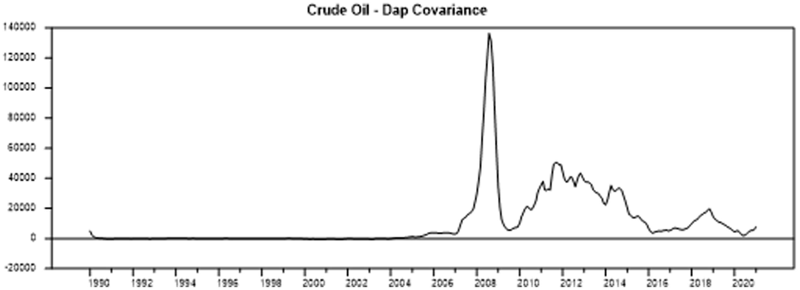
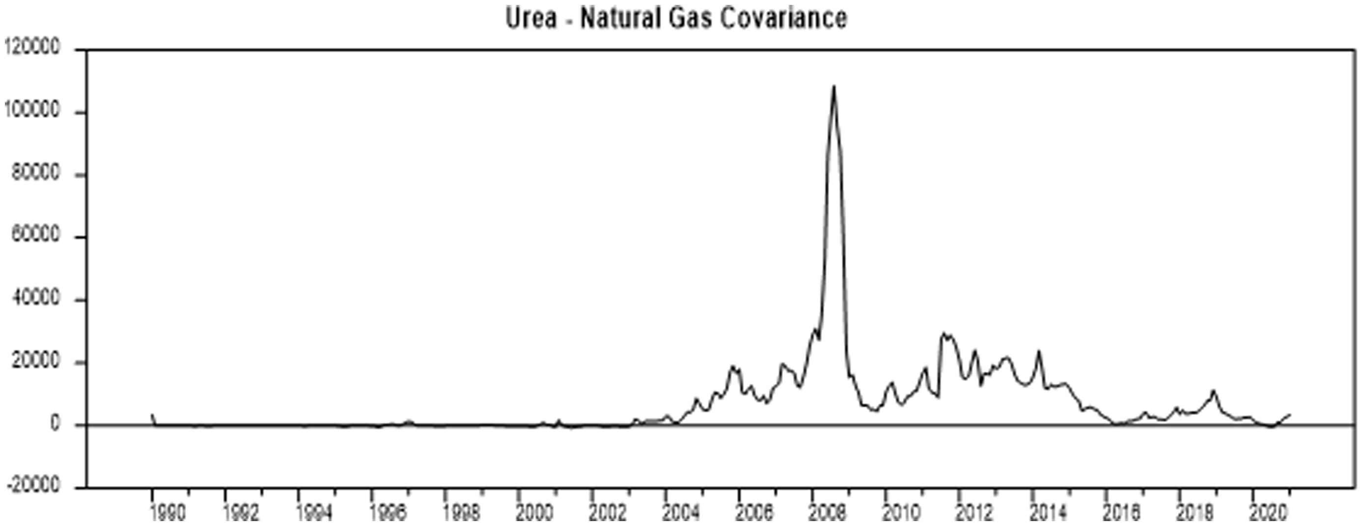
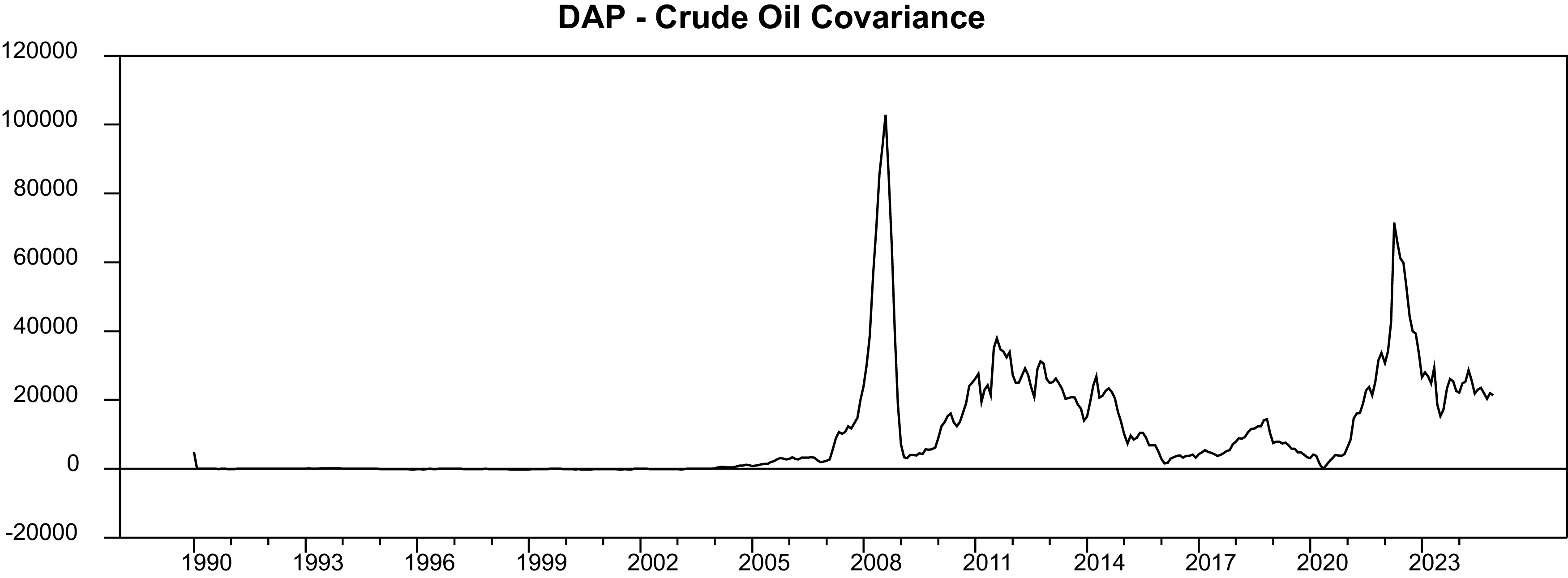
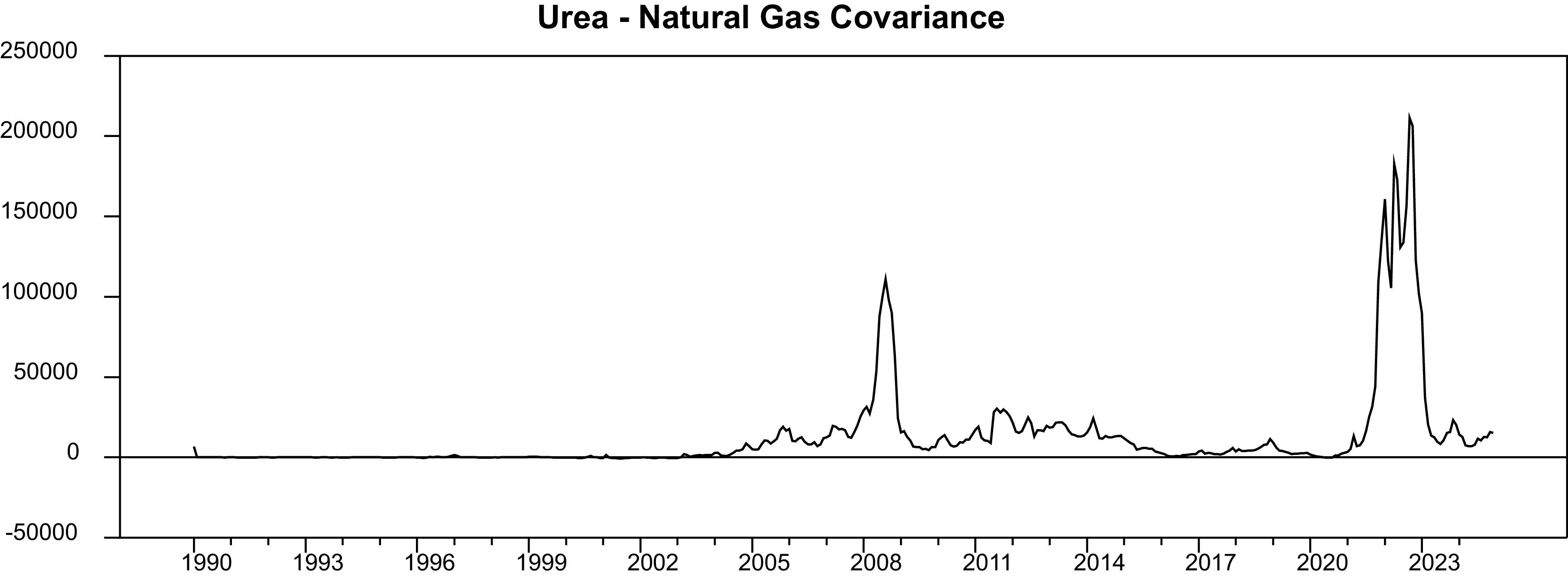
The price of Di-ammonium Phosphate (Urea) and the price of crude oil (natural gas) are both assumed to be I(0) processes in the econometric approach described above. Figures 4 and 5 show the covariance’s in detail. In light of this, it is shown that covariances accurately reflect the obvious peaks around the 2008 financial crisis and the volatile period aftermath.
Conditional covariance of crude oil and Di Ammonium phosphate.
(Source: World Bank and Authors calculations).

Conditional covariance of urea and natural gas.
(Source: World Bank and Authors calculations).

Analyzing the pairwise conditional covariances from Equations (5) and (6) the p-values (0.009 and 0.000 respectively) indicate strong statistical significance, suggesting the conditional covariance between the respective commodity pairs is dynamic and non-zero, and varies over time. Thus it is possible to confer that the conditional covariance estimates from the BEKK GARCH(1,1) model indicate significant time-varying co-movement between Crude Oil and Di-Ammonium Phosphate, and between Urea and Natural Gas. Additionally, the covariance series capture strong co-movement during systemic shocks such as the 2008 financial crisis, suggesting that external macroeconomic volatility propagates through both energy and fertilizer markets. The pattern is especially pronounced for the Urea–Natural Gas pair, reflecting the technological link via ammonia synthesis (gas-intensive), whereas the Oil–DAP pair additionally embeds broader energy-related pass-through via transport and processing costs. These facts support the hypothesis that fertilizer markets are partially integrated with global energy markets, with nontrivial implications for input price hedging and agricultural risk management.
In this framework, a high covariance between energy and fertilizer prices signifies periods of joint volatility, typically occurring during shocks (e.g., the 2008 financial crisis). During such episodes, uncertainty regarding input costs becomes more pronounced, prompting risk-averse behavior among producers and intermediaries. This behavior may manifest in the form of delayed production decisions, increased hedging activities, or restricted speculative inventory holdings, all of which can exert downward pressure on grain prices in the short term. In other words, elevated covariances act as “joint volatility states” that trigger a set of economic mechanisms – precautionary adjustment, de-stocking, and improved hedging alignment – that collectively dampen spot grain prices despite rising input costs. This interpretation, may be labeled as the “risk-intensification effect,” highlighting that stronger co-movement in input markets tempers short-run commodity price surges rather than amplifying them. Hence, the negative and statistically significant coefficients associated with conditional covariances should be interpreted as indicators of this risk – intensification effect. We should underline that, this negative effect of covariances does not contradict the positive pass-through of energy price levels into grain prices, but rather reflects an additional state variable that is activated in turbulent periods, offsetting part of the upward price pressure with a distinct short-run dampening mechanism.
Furthermore, the incorporation of conditional covariances aids in mitigating multicollinearity between energy and fertilizer price series, which are otherwise highly correlated. By capturing their joint variance dynamics within a single measure, the model avoids redundant information and improves coefficient estimation. The inclusion of covariances refines the computation of standard errors and t-statistics, as part of the heteroskedasticity is filtered out through the variance-covariance structure. In this regard, covariances serve both as an indicators of market co-movement and as econometric adjustments that improve the reliability and interpretability of the results. This dual role underscores their substantive contribution to the empirical framework.
More specifically, including conditional covariances allows the joint variance structure of the variables to be explicitly incorporated into the model. This reduces the impact of heteroskedasticity and potential autocorrelation in the residuals, leading to more accurate computation of standard errors and, consequently, more reliable t-statistics (Su and Hung Reference Su and Hung2018). Such an adjustment is particularly valuable in settings where market series exhibit high volatility and strong co-movement, as it helps to reduce parameter uncertainty and enhances the overall robustness of the estimation results (Brooks et al. Reference Brooks, Burke and Persand2003). Consistent with this interpretation, our estimates show that even relatively small negative covariance coefficients (≈−0.001) are statistically significant and state-dependent, aligning with the prediction that their magnitude should increase during high-volatility subsamples such as 2007–2010 or 2020.
A potential concern is whether fertilizer prices can be considered exogenous in the crop-price regressions, since they are strongly shaped by developments in energy markets. We address this by making the identification strategy explicit: crude oil and natural gas are treated as the primary drivers, while fertilizer prices are interpreted as contingent outcomes of energy cost pass-through. This structure reflects the technological asymmetry in production – fertilizer manufacturing is highly energy-intensive, with natural gas accounting for roughly 70% of ammonia/urea variable costs, and with the sector representing only a fraction of the scale of global oil and gas markets. Ammonia production accounts for about 2% of global final energy use, while the oil and gas market is much larger and deeper. Given these scale differences, feedback from fertilizers to energy is regarded as economically and theoretically negligible.
Within this framework, fertilizers are not modeled as independent shocks but as transmission channels of energy into agriculture. To further limit spurious attribution, the baseline already controls for oil and gas prices directly and incorporates conditional covariances between energy and fertilizers, ensuring that fertilizer coefficients are interpreted net of contemporaneous energy shocks. This treatment acknowledges the close link between the two markets while remaining consistent with the one-way cost-push causality from energy to fertilizers and to grains.
As mentioned earlier, the effects of the post-2021 crisis are reflected in the covariance dynamics presented in Appendix Figure 2. Although the covariances – i.e., co-movements – between DAP and crude oil exhibit a similar pattern to those between urea and natural gas, the magnitude of the urea – natural gas covariance is considerably higher. It is worth noting that in contrast to the 2007 crisis, the 2021 crisis has not yet stabilized, which accounts for the heightened volatility observed in both covariance measures. Moreover, it should be noted that the descriptive statistics and standard unit root test results provided in the section are based on the full sample, while the main statistical properties and test results of the variables are valid for both samples.
Results
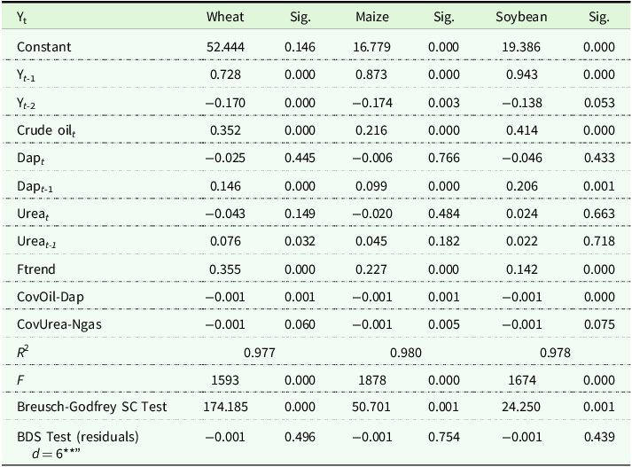
The stochastic time series characteristics are assessed to identify the most consistent model with the data. The results show that the time series in concern is governed by time-dependent non-linear Fourier trends. When these features are accounted for the series becomes stationary and there is no need for differencing. Then the conditional covariances (Crude oil-DAP, NGas-Urea) are obtained from BEKK GARCH (1,1) to employ them in the final model. Finally, the equation stated below could be estimated by ordinary least squares (OLS).
 $${Y_{{x_i},t}} = {\alpha _{{x_i}}} + \mathop \sum \nolimits_{j = 1}^n {\beta _i}{Y_{xi,t - j}} + \mathop \sum \nolimits_{j = 1}^k {C_j}\ {\rm{Crudeoi}}{{\rm{l}}_{t - j}} + \mathop \sum \nolimits_{j = 1}^m {H_j}{\rm{DA}}{{\rm{P}}_{t - j}} + \mathop \sum \nolimits_{j = 1}^r {G_j}{\rm{URE}}{{\rm{A}}_{t - j}} + {\rm{Ftren}}{{\rm{d}}_{xi,t}} + {\rm{CO}}{{\rm{V}}_{Oil - dap,t}} + {\rm{CO}}{{\rm{V}}_{urea - ngas,t}} + {\varepsilon _t}\;$$
Equation (7) will be estimated separately for wheat, maize, and soybean. Here Yxi gives wheat, maize, and soybeans with lags on the right-hand side. Cj is used for crude oil, Hj for Di-ammonium Phosphate, and Gj for Urea prices with necessary lags. The Fourier trend is depicted by Ftrend and the co-movements (covariances) of crude oil-dap and Urea-natural gas are also given by COV parameters.
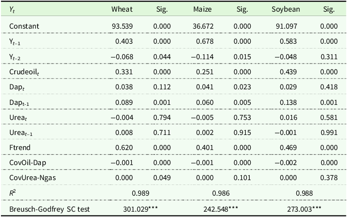
The estimation results of Equation (7) are given in Table 6:
Estimation results*

*To account for serial correlation, the Newey-West adjusted standard errors are used and robust or HAC standard errors are obtained.
**Bootstrap probabilities with 2500 iterations are used. Only dimension 6 is reported.
Source: Authors calculations.
Here, the nonlinearity Broock–Dechert–Scheinkma (BDS) approach (Brock et al. Reference Brock, Dechert, LeBaron and Scheinkman1996) has been selected to identify the residuals derived from Equation (7). The null hypothesis in the BDS test with independent and identical distribution was accepted (Table 6), indicating that the time series does not exhibited nonlinear characteristics across various dimensions. This indicates that the Fourier trend resolved the nonlinearity. The modelFootnote 3 solves serial correlationFootnote 4 and non-linear trend problems. Rather than being non-stationary, the series involved in this study are governed by non-linear trend structures. The coefficients of the Fourier trends do not exhibit big differences across the commodities (0.355, 0.227, 0.147 in wheat, maize, and soybeans respectively) and are significant in all cases. In the estimation equation log-specified variables are interpreted as elasticities; conditional covariance coefficients are interpreted in levels as state-dependent co-movement indicators. The estimated coefficients for the conditional covariances, although small in magnitude (–0.001 across all cases), are statistically significant and indicate that even minor fluctuations in the co-movements between energy and fertilizer markets have a measurable effect on grain prices. The negative and significant effect of the CovOil-DAP term across wheat, maize, and soybeans suggests that when crude oil and di-ammonium phosphate prices move more closely together. This relatively closer co-movement has a potential to dampen commodity price increases. This could reflect increased uncertainty in input markets during global shocks, such as the 2008 financial crisis, leading to risk-averse behavior among producers. Similarly, the Cov(Urea-NGas) term is negative and statistically significant for maize, marginally significant for wheat, and borderline significant for soybeans, indicating that higher co-movement between urea and natural gas prices may also contribute to downward pressure on grain prices. The statistical significance of these coefficients highlights that co-movements between markets contain important information about the dynamics of commodity price formation. This underscores the importance of considering not just price levels, but also the relationships between input markets (and for that matter the input price volatility) when analyzing agricultural price behavior. Using the appropriate trend structures in the wheat, maize, and soybean price equation, it is found that the conditional covariance between energy and fertilizer markets has a significant role in price determination. In all cases the coefficients of conditional covariances are very low and also significant. The two lags of the dependent variable used in the estimation are significant in all cases. The coefficient of crude oil price is significant for wheat, maize, and soybean and directly affects prices. Especially the crude oil coefficient is high in soybean with 0.414, wheat with 0.352, and maize with 0.217. Even though the highly subsidized nature of soybean and maize is considered, one can say energy plays a crucial role (directly and indirectly) in the price formation of these commodities. DAP fertilizer also plays a crucial role. As seen from the estimation results, at time t, the DAP coefficient is negative in contrast to expectations (−0.025, 0.006, −0.046 for wheat, maize, and soybeans respectively) but it is insignificant in all cases. The coefficient turns out to be expected positive in the first lag. This shows that price changes in the DAP fertilizer are positively transferred to the prices of wheat, maize, and soybeans with one lag. The Urea fertilizer follows similar patterns with DAP in wheat. A price change in Urea is positively affecting the price of wheat after one lag. The results are interesting for maize and soybean. Although the coefficients are positive in all used lags, they are insignificant. This can be a result of the heavily subsidized nature of maize and soybean globally.
The findings show that energy plays a crucial role in the price determination of selected grains. The crude oil parameter is positive and significant in all cases. There is almost an immediate impact of a change in the price of crude oil over commodity prices. The DAP fertilizer is positive and significant in the second lag. This suggests that a change in the price of oil first affects the price of fertilizer before eventually affecting the price of commodities. The effect of a price change in Urea fertilizer moves similarly with DAP fertilizer except in maize and soybeans although the coefficients are small.
The fertilizer coefficients should therefore be interpreted as marginal effects, conditional on the inclusion of energy prices and covariance terms. In other words, they capture the additional pass-through from fertilizers to grains once direct energy influences have been accounted for. This means that fertilizer effects primarily reflect lagged transmission of input-cost pressures rather than independent exogenous variation.
The urea shock was particularly severe because nitrogen fertilizers – unlike phosphate – are overwhelmingly gas-based. Many studies point out that natural gas accounts for a hefty share of variable costs in ammonia/urea production, compared with a smaller portion of oil-linked inputs in diammonium phosphate (DAP) (see Duhalt Reference Duhalt2018; Heffer and Prud’homme Reference Heffer and Prud’homme2016; IFA 2023). This explains why rising natural gas prices translated disproportionately into urea costs, reinforcing the tight coupling of urea and gas in sample.
However, the transmission weakened over time due to adaptive responses and policy interventions. Agricultural producers substituted away from nitrogen fertilizers, particularly from urea, toward alternative inputs or adopted more efficient application practices, while governments in both advanced and developing economies deployed subsidy programs, tariff suspensions, and emergency procurement to shield domestic producers from global price volatility (FAO 2022; OECD/FAO 2022). Moreover during this period, fertilizer markets moved from a single-crisis environment in 2008 into a broader polycrisis setting by 2022. While the immediate fertilizer shock moderated, global agriculture was hit simultaneously by energy volatility, El Niño–linked weather extremes, food export bans, and Red Sea shipping disruptions (Bogetic et al. Reference Bogetic, Zhao, Le Borgne and Krambeck2024; FAO 2023). This compounded shock environment fogs the outlook and hence the transmission channels. Meanwhile, as Europe diversified LNG imports and additional fertilizer capacity came online in other regions, natural gas markets stabilized in 2023–2024 easing pressure on urea prices (IFA 2023). Consequently, the explanatory power of urea in grain-price equations has relatively declined. It is worth noting again that in the post-2022 period, their role as the dominant conduit of energy shocks was superseded/overpowered by multiple overlapping crises and broader supply-chain pressures. Thus, although the dataset extends until December 2024, the empirical analysis in this paper concentrates on the period up to February 2021.
The subsequent period is characterized by the outbreak of the Russian–Ukrainian War and the emergence of overlapping shocks in energy, fertilizer, and food markets. These ongoing disruptions represent a polycrisis environment marked by unresolved supply chain bottlenecks, export restrictions, input price spikes, and unprecedented policy interventions. Because these dynamics have yet to reach a resolution, their inclusion obscures the underlying structural relationships that this study seeks to uncover. Focusing on the pre–Russian–Ukrainian War period therefore ensures that the estimated effects reflect more fundamental mechanisms, as opposed to transitory, war-specific shocks, and provides a clearer foundation for interpreting both the direct and indirect linkages between energy and agricultural markets. Nevertheless, the full-sample analysis and results are reported in the annex section of the study.
We should note that when the dataset is extended beyond 2021 to include the ongoing Russian-Ukrainian War from February 2022 to end of 2024, the previously strong indirect channel from natural gas to crop prices via urea becomes weaker. This result might be attributed to several structural developments in global fertilizer markets. The Russian–Ukrainian war triggered an unprecedented surge in urea prices, as Russia and Belarus – both key exporters of nitrogenous fertilizers – faced sanctions and supply disruptions (FAO/WTO 2022). FAO/WTO (2022) calculations based on Trade Data Monitor data display a rather stable trend of Russian exports, indicating a significant decline in export volume, as the prices were almost tripled between 2020 and 2022. Hence, initially, this shock amplified input costs for grain production, consistent with our earlier results.
Discussion & conclusion
Agriculture has become industrialized, specialized, and integrated. In many nations, production shifts from family-based, small-scale agriculture to industrial-style agricultural institutions that rely more heavily on energy utilization. Therefore, it is not wrong to state that modern agriculture is distinguished by energy-intensive mass production and high input utilization through national input markets that are connected to global sourcing, particularly in developing countries.
It is clear that a variety of factors, including the drought, have an impact on agricultural productivity and prices. However, it is also true that all aspects of modern intensive farming, including production, processing, transportation, etc., are directly related to energy. Enhanced seeds used in the cultivation of wheat, maize, and soybeans are more responsive to industrial inputs such as inorganic fertilizers, pesticides, and fuel, among others. These new, higher-yielding varieties require larger amounts of fertilizer. However, prolonged use of synthetic fertilizer leads to soil degradation, necessitating even greater quantities of fertilizer to maintain productivity. Since the manufacturing and transportation of DAP rely on crude oil, and urea relies on natural gas, higher fertilizer production increases the demand for energy. As production scales up, the demand for improved mechanization, such as powerful tractors and harvesters, also increases. The use of mechanization equipment, such as tractors and harvesters, is energy-intensive. Therefore, this higher level of mechanization and technological advancements results in a greater demand for fuel. Furthermore, the processing and distribution to end users also require complex transportation systems that rely on energy both domestically and internationally. Thus, the study’s findings are consistent with the dependance of agricultural production on energy. Improvements in energy markets directly (crude oil) transmits to grain prices and indirectly (crude oil and ngas) through inputs (fertilizers). The results of this study are consistent with this interpretation: energy prices remain the dominant direct driver of grain prices, while fertilizer effects materialize with lags and in interaction with energy volatility. This supports the economic view that fertilizers act as a secondary propagation channel of energy shocks into agricultural markets, rather than as autonomous sources of price formation. Moreover, results show that covariance effects are economically small in tranquil periods but substantively larger during high-volatility episodes, consistent with the joint-volatility (risk-intensification) interpretation.
The international prices of major agricultural commodities have been consistently increasing, influenced by various factors such as supply and demand shocks. Energy, in particular, plays a significant role in this trend. Countries that rely on imported oil, agricultural commodities, or fertilizers for domestic agricultural production may consequently become dependent on energy for their agriculture. When a country relies on foreign sources for agricultural inputs, it is impossible to avoid fluctuations in international energy markets. Consequently, these fluctuations in international energy prices will inevitably impact domestic prices. Therefore, the dependency of agriculture on energy prices makes them vulnerable to changes and crises in energy markets. As a result, policymakers should implement several measures to mitigate the impact of energy price fluctuations on agricultural production and productivity. To ensure long-term stability, it is necessary to undergo structural transformations that reduce dependance on energy. For example, through an examination of the energy dependance structure and adverse environmental impacts of chemical fertilizers, the reduction of their utilization can be accomplished by increasing farmers’ awareness and advocating for the use of organic fertilizers, such as compost, which are sourced from domestic resources and have lower energy requirements.
Maintaining price stability for agricultural commodities is of strategic importance on a global scale. Therefore, in response to concerns regarding food price inflation and the unintended environmental consequences of energy-intensive farming, stringent policy measures must be implemented worldwide in the coming years to decrease energy consumption in agricultural commodities and the use of agricultural commodities for energy.
Finally, the study’s findings indicate that the coefficients are as expected, and that non-linear trends and conditional covariances should be incorporated in future work to accurately measure the stationarity properties of commodity prices. Furthermore, during volatile times, conditional covariance between markets tends to increase. As a result, the covariance effect becomes especially relevant during such crises and should be carefully considered when creating strategies in response to the crisis. Accordingly, future research should revisit and extend this analysis once the current polycrisis period has subsided (Appendix of this study provides initial results even though the polycrisis period is yet to end), so that results can be evaluated under these market conditions and disentangled from the extraordinary ongoing shocks that dominate the recent subsample.
Data availability statement
The data that support the findings of this study are available from publicly accessible sources and compiled by the authors. The data and code used in this study are available upon request from the corresponding author. There are no restrictions on access.
Acknowledgements
The authors gratefully acknowledge Prof. Dr. Tolga Omay for his invaluable support, insightful comments, and thoughtful suggestions during the preparation of this manuscript. His expertise and guidance played an important role in shaping the paper. Any remaining errors are, of course, the authors’ own.
Funding statement
This research received no specific grant from any funding agency, commercial or not-for-profit sectors.
Competing interests
The authors declare no competing interests.
Appendix
The descriptive statistics of the variables for the extended sample range (1991–2024) are presented in Appendix Table 1.
Descriptive statistics

Source: Authors calculation.
The standard unit-root test results are reported in Appendix Table 2. These indicate that the fertilizer series (DAP and Urea) are stationary in levels, whereas the remaining variables are integrated of order one I(1).
Unit root test results

Notes: *1%, **5% and ***10%, Critical values for Dickey-Fuller and Philips-Perron are −3.446, −2.868,−2.570 (1%,5%,10% respectively).
The results of additional unit root tests are reported below in Appendix Table 3. To capture potential nonlinear (state- or time-dependent) dynamics, The Leybourne, Newbold, and Vougas (LNV, 1998) and Kapetanios, Shin, and Snell (KSS, 2003) test results once again show that the LNV model-b provides the better fit, while the wheat, maize, and soybean series remain statistically insignificant.
Unit root test results
Notes: *1%, **5% and ***10%.
1-raw data; 2-De-meaned; 3-De-meaned and de-trended; 4-Lnv Model-a; 5-Lnv Model-b; 6-Lnv Model-c.
Critical values for KSS – raw data −2.82, −2.22, −1.92; De-meaned, −3.48, −2.93, −2.66; De-trended, −3.93, −3.40,−3.13 (1%,5%,10% respectively).
Critical Values for LNV – Model a, −4.88,−4.23,−3.91; Model b, −5.48, −4.77, −4.43; Model c, −5.65, −5.01, −4.70 (1%,5%,10% respectively).
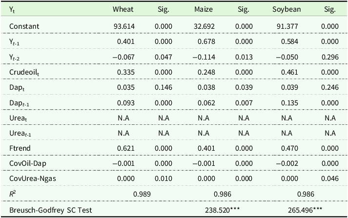
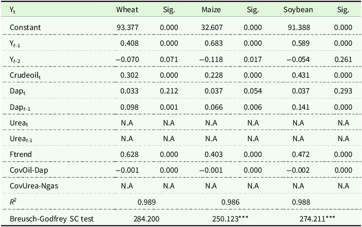
Estimation results for the Equation (7)’s alternative identifications are provided in Appendix Table 4, Appendix Table 5 and Appendix Table 6, respectively. In the analysis conducted with the extended data, the Fourier frequency increased by one (k = 4) according to the AIC.
Estimation results for Equation (7) using Alternative Identification Strategy 1

Notes: *1%, **5% and ***10%.
Estimation results for Equation (7) using Alternative Identification Strategy 2

Notes: *1%, **5% and ***10%.
Estimation results for Equation (7) using Alternative Identification Strategy 3

Notes: *1%, **5% and ***10%.
DAP Crude Oil Covariance.

Urea Natural Gas Covariance.


 Open access