


1 Introduction
The computation of viscous flow in channels of varying cross-section continues to be of significant interest. As indicated by Shub [Reference Shub24], there are several industrial applications involving channels for which the cross-sectional area varies periodically in the streamwise flow direction. One such application concerns the development of smaller cooling devices, which require outflow pipes with enhanced heat-exchange properties, and this is discussed by Sui et al. [Reference Sui, Teo and Lee26]. Invariably, numerical methods are needed to solve these problems, because the Navier–Stokes equations of viscous fluid flow are difficult and nonlinear, and, in addition, the irregular shapes of the oscillatory channel walls make the imposition of boundary conditions particularly difficult. Accordingly, many authors have employed finite-difference or finite-element methods to give the numerical solutions they require. One such example is the article by Wang and Chen [Reference Wang and Chen33] who transform the Navier–Stokes equations to a nonorthogonal boundary-fitting coordinate system and obtain solutions using finite differences. An interesting alternative to these techniques is provided by Al-Zoubi and Brenner [Reference Al-Zoubi and Brenner1], who used a lattice-Boltzmann method to solve for flow in which the oscillations only appeared on one wall of the channel, in an application from lubrication theory. Other general approaches include body-fitted unstructured meshes [Reference Ferziger and Perić12] and spectral element methods [Reference Patera20].
A numerical solution for two-dimensional incompressible fluid flow in a channel having periodically oscillating walls is presented by Bahaidarah and Sahin [Reference Bahaidarah and Sahin2]. They consider a channel in which both the top and bottom walls vary sinusoidally with the same wavelength, creating a varicose channel with wide and narrow segments alternating in the flow direction x. They generated a nonrectangular grid system by scaling the other coordinate y to make it fit to the upper and lower channel walls at each value of x. A computer package then solved the transformed equations. In the cases they considered, a steady-state flow configuration was evidently achieved within a few wavelengths in x.
Two types of periodic oscillatory wall shapes were considered by Nishimura and Matsune [Reference Nishimura and Matsune18], and, similarly to the work of Bahaidarah and Sahin [Reference Bahaidarah and Sahin2], they allowed oscillatory structures of the same wavelength on both walls. One of their configurations was also a varicose structure, in which the oscillations on the top wall were of the opposite phase to those on the bottom wall. Their second configuration required the oscillations on both walls to have the same phase, giving a serpentine-shaped outflow channel. They solved their equations for unsteady pulsatile incompressible flow using a finite-element scheme, and showed the presence of detached vortices for both channel types. Interestingly, they observed that heat and mass transfer in the oscillatory channel are enhanced significantly by the presence of large-amplitude fluid oscillations; from the mathematical point of view, this is precisely the nonlinear domain, and so underscores the importance of reliable, accurate numerical solutions. A similar remark is offered by Cho et al. [Reference Cho, Kim and Shin8], who highlight the influence that the geometric shape of the walls can have, and that possibly internal vortex generation may be a large factor in this.
If there are no oscillations on the channel walls, a steady-state flow is, of course, possible. This is simply the well-known plane Poiseuille flow (see Batchelor [Reference Batchelor3, page 183]) in which the fluid speed u is parabolic in y and falls to zero at the two walls. When the walls vary periodically in x, however, the question arises as to whether a stable steady flow continues to exist. An experimental study by Nishimura et al. [Reference Nishimura, Bian, Matsumoto and Kunitsugu17] did indeed find steady flows for sufficiently small Reynolds number. Linearized analyses have been carried out by Selvarajan et al. [Reference Selvarajan, Tulapurkara and Vasanta Ram22], and later by Trifonov [Reference Trifonov29], who computed a steady numerical solution for a two-dimensional flow in a corrugated channel, and then assessed the linear stability when small disturbances are applied by carrying out a rather comprehensive eigenvalue and Floquet analysis numerically.
The treatment of the boundary conditions on the undulating channel wall(s) is the most difficult numerical task. Perhaps the simplest way of approaching this is to scale a coordinate transverse to the walls; thus, if the two channels walls are at
 $y=f_L(x)$
and
$y=f_L(x)$
and
 $y=f_U(x)$
, then a new coordinate
$y=f_U(x)$
, then a new coordinate
 $\eta = ( 2y - f_U - f_L ) / ( f_U - f_L )$
takes the value
$\eta = ( 2y - f_U - f_L ) / ( f_U - f_L )$
takes the value
 $\eta = -1$
at
$\eta = -1$
at
 $y = f_L$
and
$y = f_L$
and
 $\eta = 1$
at
$\eta = 1$
at
 $y = f_U$
. This creates a rectangular domain in the
$y = f_U$
. This creates a rectangular domain in the
 $( x , \eta )$
coordinates, and now standard numerical approaches can be applied. Trifonov [Reference Trifonov29] adopted this scheme, as did Cho et al. [Reference Cho, Kim and Shin8] and Wang and Chen [Reference Wang and Chen33], along with many others. It should be noted that the
$( x , \eta )$
coordinates, and now standard numerical approaches can be applied. Trifonov [Reference Trifonov29] adopted this scheme, as did Cho et al. [Reference Cho, Kim and Shin8] and Wang and Chen [Reference Wang and Chen33], along with many others. It should be noted that the
 $( x , \eta )$
variables form a nonorthogonal coordinate system. This is likely to be of little concern for small-amplitude channel oscillations, but its reliability for large wall oscillations remains uncertain, where it might conceivably result in ill conditioning should the angle between coordinates become small. In a variant of this approach, Kaliakatsos et al. [Reference Kaliakatsos, Pentaris, Koutsouris and Tsangaris15] used an artificial compressibility technique, in which a steady incompressible channel flow was computed by allowing the fluid density to vary with time, and then integrating forward in time until the density became constant.
$( x , \eta )$
variables form a nonorthogonal coordinate system. This is likely to be of little concern for small-amplitude channel oscillations, but its reliability for large wall oscillations remains uncertain, where it might conceivably result in ill conditioning should the angle between coordinates become small. In a variant of this approach, Kaliakatsos et al. [Reference Kaliakatsos, Pentaris, Koutsouris and Tsangaris15] used an artificial compressibility technique, in which a steady incompressible channel flow was computed by allowing the fluid density to vary with time, and then integrating forward in time until the density became constant.
An alternative scheme for coping with irregularly shaped channel walls is to embed the physical region within a larger rectangular coordinate system. This idea has been used for inviscid fluids with interfaces for some time, and involves regarding the unknown interface as a level curve of some higher-dimensional function. A review of these “level set methods” is given by Sethian and Smereka [Reference Sethian and Smereka23]. For viscous fluids in irregularly shaped regions, a somewhat equivalent approach is the use of “fictitious domain” methods, in which the equations are solved in some larger “fictitious” domain, and the boundary conditions on the true domain are imposed using a Lagrange-multiplier technique. Glowinski et al. [Reference Glowinski, Pan and Periaux13] give examples of the computation of viscous flows using this method. “Overset grid methods” invoke a similar philosophy, and Vreman [Reference Vreman31] points out that the use of a rectangular grid carries a number of numerical advantages. A review of some aspects of the computation of nonlinear flows using a fictitious domain method is presented by Yu and Shao [Reference Yu and Shao34]. A somewhat more controversial scheme of this type has been developed for flows in irregular channels by Szumbarski and Floryan [Reference Szumbarski and Floryan27]. It expresses the solution in spectral form as Fourier series, but imposes boundary conditions along some curve within the fluid region. The authors had success with this approach, but caution that it probably cannot be guaranteed to succeed in all cases. Boyd [Reference Boyd7] suggests that their method relies so heavily on analytic continuation that it would, in general, be subject to creating false internal singularities and branch lines, and thus be likely to fail. The fact that it did not is attributed, by Boyd [Reference Boyd7], to divine benevolence.
In principle, the most precise way of enforcing the boundary conditions, in two-dimensional flow, is to use conformal mapping. The irregularly shaped fluid domain would be mapped to a rectangular one, in which numerical schemes could then impose correct boundary conditions exactly. However, it is usually not possible to do the conformal mapping in closed form, so that a numerical mapping would be needed for an arbitrary wall shape. For inviscid fluids, King and Bloor [Reference King and Bloor16] developed a numerical Schwarz–Christoffel technique, which they used to solve for free-surface flows under gravity, over bottom topography. The Schwarz–Christoffel mapping is not always straightforward to implement, however, since it introduces branch lines as part of the technique. Rivera-Alvarez and Ordonez [Reference Riviera-Alvarez and Ordonez21] instead solved Laplace’s equation to perform their conformal mapping numerically, so as to study viscous flow in a wavy channel.
After conformal mapping has been performed, the task is now to carry out the numerical solution of the nonlinear fluid equations in a simple periodic (mapped) domain. The finite-difference and finite-element techniques discussed above are certainly available for this purpose, but, in these simple geometries, global spectral methods are well known to be highly accurate, with exponential convergence for quadratures, and for matching boundary conditions. Details are given in the book by Boyd [Reference Boyd6]. The purpose of this current paper is therefore to present a novel but straightforward method for implementing global spectral methods to combine conformal mapping with equation solving, to solve the Navier–Stokes equations in an arbitrary smooth periodic two-dimensional channel.
The current work is presented in two halves. In the first half, the spectral method is set out for a straight channel, choosing appropriate basis functions for the no-slip walls, and describing the treatment of pressure, continuity and the Navier–Stokes equations, as well as the time-stepping method. The second half introduces conformal mapping to allow a periodic channel section with a smooth wavy wall to be mapped to a rectangular region. The equations are transformed using this mapping, and then the straight-channel algorithm is applied, with the mapped equations.
In the first half, the method is carefully checked against known or analytic solutions. These are generally not available in the case of a wavy channel. However, lubrication theory predicts the amount of drag due to such wall undulations, so these are used to check the accuracy of the numerics for laminar flow. In the case of high Reynolds’ number flow, a convergence study has been presented, along with some benchmarking data so that other methods may be compared with the one presented here.
Following this introduction, the paper is presented as follows. Section 2 lays out the methodology for solving unsteady flow in a two-dimensional straight-walled channel section, describing governing equations, boundary conditions and related basis functions, treatment of the pressure term and the numerical approach. In Section 3, this numerical scheme is tested against analytic solutions for unidirectional channel flow, and for vortices in the creeping flow limit, as well as a qualitative check of nonlinear decay rate for a pair of counter-rotating vortices. Section 4 introduces conformal mapping for a wavy-walled channel, and the governing equations are transformed via this mapping. Section 5 presents a comparison with the predictions from lubrication theory, and Section 6 shows numerical results for some simple wall shapes, finishing with a high Reynolds’ number (
 $Re=10^5$
) flow through a wavy-walled channel. Final remarks and suggestions for future work are given in the conclusion.
$Re=10^5$
) flow through a wavy-walled channel. Final remarks and suggestions for future work are given in the conclusion.
2 Planar channel: spectral-Galerkin framework
In this section, we present a spectral-Galerkin formulation for the flow of a homogeneous, incompressible fluid in a two-dimensional channel with straight rigid walls. The focus here is to develop the structure of the chosen numerical method, and to validate it in this well-known geometry, by testing accuracy against some known solutions of the flow equations. Doing so allows us to move into more arbitrary channel shapes with confidence that each element of the solution scheme is functioning correctly. This method will be reused when nonrectangular geometries are considered.
The format of this section is as follows. First, the equations governing the flow are presented in the form of the continuity equation, the streamwise momentum equation and the vorticity transport equation. These are nondimensionalized to reduce the number of independent parameters. The streamfunction is then introduced to satisfy continuity implicitly. Pressure is treated as an auxiliary quantity required for solving the momentum equation, so its Poisson equation and corresponding solution method are then described. Next, boundary conditions for both velocity and pressure are described and met exactly through the construction of suitable basis functions. These bases are used to transform between spectral and physical space, facilitating accurate and efficient integration of the governing equations. The time-stepping integration scheme is then explained, followed by details of the numerical approach to be taken.
2.1 Flow equations
For incompressible flow in two dimensions, the governing equations are the continuity equation (incompressibility condition)
 $$ \begin{align} \nabla \cdot \mathbf{q} = 0 \end{align} $$
and the Navier–Stokes (momentum) equation, which balances forces per unit volume,
 $$ \begin{align} \rho \bigg(\frac{\partial \mathbf{q}}{\partial t} + (\mathbf{q} \cdot \nabla) \mathbf{q}\bigg) & = -\nabla P + \mu \nabla^2 \mathbf{q} + \mathbf{f}. \end{align} $$
In these equations, q = (u, v) is the velocity field,
 $\rho $
is the (constant) density, P is the pressure field, μ is the dynamic viscosity and f = ρ
g is the gravity forcing term, with gravitational acceleration g = g(sin(θ)î − cos(θ)ĵ). That is, the channel is rotated clockwise from the horizontal by an angle
$\rho $
is the (constant) density, P is the pressure field, μ is the dynamic viscosity and f = ρ
g is the gravity forcing term, with gravitational acceleration g = g(sin(θ)î − cos(θ)ĵ). That is, the channel is rotated clockwise from the horizontal by an angle
 $\theta $
. The pressure gradient in this equation is dependent on the velocity field, and must be calculated at each time step. This will be described in detail below. In seeking a stable numerical solution it is convenient to take the curl of the momentum equation to yield the vorticity equation
$\theta $
. The pressure gradient in this equation is dependent on the velocity field, and must be calculated at each time step. This will be described in detail below. In seeking a stable numerical solution it is convenient to take the curl of the momentum equation to yield the vorticity equation
 $$ \begin{align} \frac{\partial \omega}{\partial t} + (\mathbf{q} \cdot \nabla) \omega & = \frac{\mu}{\rho} \nabla^2 \omega. \end{align} $$
The scalar vorticity is defined to be
 $\omega =\partial v/\partial x-\partial u/\partial y$
.
$\omega =\partial v/\partial x-\partial u/\partial y$
.
Considering a rectangular channel section,
 $-L \pi <x<L\pi $
,
$-L \pi <x<L\pi $
,
 $-H<y<H$
, we now introduce dimensionless variables, by scaling with the half-height H of the channel, the density
$-H<y<H$
, we now introduce dimensionless variables, by scaling with the half-height H of the channel, the density
 $\rho $
and the centreline Poiseuille velocity
$\rho $
and the centreline Poiseuille velocity
 $U_c$
. This velocity is calculated by considering one-dimensional steady flow, with the channel rotated for maximum flow (
$U_c$
. This velocity is calculated by considering one-dimensional steady flow, with the channel rotated for maximum flow (
 $\sin \theta =1$
). In this case, the momentum equation simplifies to
$\sin \theta =1$
). In this case, the momentum equation simplifies to
 $$ \begin{align*} 0=\rho g+\mu \frac{\partial^2 u}{\partial y^2}, \end{align*} $$
in which u is the velocity component along the channel. Applying boundary and symmetry conditions gives the velocity on the centreline (
 $y=0$
) to be
$y=0$
) to be
 $$ \begin{align*} U_c=u(0)= \frac{\rho g}{2 \mu}H^2. \end{align*} $$
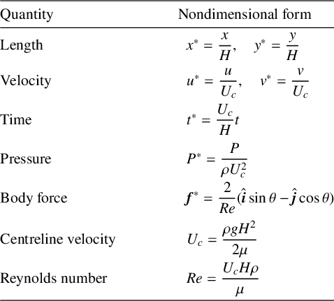
Although it may be unusual to define the centreline velocity in this way, it is convenient for the analysis that follows, resulting in the simplest form for the Poiseuille flow. This is an arbitrary choice for the current work. The nondimensionalization of the variables is shown in Table 1.
Nondimensionalization for gravity-driven Poiseuille flow down a sloped channel.
Employing these new variables, but removing the stars for readability, equation (2.2) becomes
 $$ \begin{align} \frac{\partial \mathbf{q}}{\partial t} + (\mathbf{q} \cdot \nabla) \mathbf{q} & = -\nabla P + \dfrac{1}{Re}\nabla^2 \mathbf{q} + \dfrac{2}{Re}(\hat {\boldsymbol i} \sin \theta-\hat {\boldsymbol j}\cos \theta), \end{align} $$
on a grid
 $-S \pi <x<S\pi $
,
$-S \pi <x<S\pi $
,
 $-1<y<1$
, for scale factor
$-1<y<1$
, for scale factor
 $S=L/H$
.
$S=L/H$
.
2.2 Streamfunction formulation
To enforce incompressibility, we introduce the streamfunction ψ. Using subscripts to denote partial derivatives,
 $\psi $
is related to the velocity components by
$\psi $
is related to the velocity components by
 $$ \begin{align*} u = \psi_y, \quad v = -\psi_x, \end{align*} $$
which automatically satisfies the incompressibility condition (2.1).
The velocity field is fully determined by the streamfunction, and thus we need to compute only ψ, which simplifies the formulation of the problem.
2.3 PPE
With flow in a channel, we can conceptually differentiate between the average streamwise velocity and the velocity components relating to the vorticity. The solution requires both parts. Although the vortical components may be determined from the vorticity equation, in which the pressure term has been removed via the curl operator, the average streamwise components require knowledge of the pressure gradient. The issue of how to deal with this pressure gradient term in the momentum equation remains an active area of interest. Arguably, it has been one of the most difficult and fundamental challenges in numerical fluid flow modelling. Unlike velocity, pressure does not have an explicit evolution equation, but must be determined through its coupling with the velocity field, leading to iterative procedures in primitive variable formulations. Various procedures have been developed to handle this coupling, including staggered-grid schemes [Reference Harlow and Welch14], projection methods [Reference Chorin9] and pressure-correction iterative schemes [Reference Patankar and Spalding19].
In this work, we use a streamfunction which solves the continuity equation identically by construction. With the pressure Poisson equation (PPE) no longer needing to enforce continuity, the complexities involved with pressure–velocity coupling may be sidestepped, and the pressure calculated explicitly at each stage of the Runge–Kutta (RK) method. We have used a one-step direct spectral method, avoiding iterative procedures, but any suitable Poisson solving technique may be used. An advantage of this approach is that high-order temporal integrators may be employed in a straightforward way.
The PPE, is derived in the normal way, from the divergence of the Navier–Stokes equation combined with the incompressibility condition. In nondimensional form, this is
 $$ \begin{align*} \nabla^2 P & = - (u_x^2+2u_y v_x+v_y^2), \end{align*} $$
noting that
 $u_x^2=v_y^2$
by the incompressibility condition. The important point is that the pressure Laplacian is dependent only on the current velocity components. Because the pressure boundary conditions are also dependent on the current velocity, the pressure may be determined at any time, and the pressure gradient can be calculated and applied to the momentum equation to determine the instantaneous acceleration field. No iterative procedure is necessary. This greatly simplifies the algorithm, avoiding the need for convergence criteria and tolerance tuning.
$u_x^2=v_y^2$
by the incompressibility condition. The important point is that the pressure Laplacian is dependent only on the current velocity components. Because the pressure boundary conditions are also dependent on the current velocity, the pressure may be determined at any time, and the pressure gradient can be calculated and applied to the momentum equation to determine the instantaneous acceleration field. No iterative procedure is necessary. This greatly simplifies the algorithm, avoiding the need for convergence criteria and tolerance tuning.
Boundary conditions are derived by taking the dot product of the boundary normal with the momentum equation. Using vector notation, this is
 $$ \begin{align*} \boldsymbol n\cdot\boldsymbol \nabla P=\boldsymbol n\cdot \bigg(\mathbf{f}-\frac{\partial \boldsymbol q}{\partial t} - ( \boldsymbol q \cdot \boldsymbol \nabla)\boldsymbol q+ \frac{1}{Re}\nabla^2 \boldsymbol q \bigg) \quad \text{on walls.} \end{align*} $$
With incompressible fluid (
 $\nabla \cdot \mathbf {q} = 0$
) and no-slip walls (
$\nabla \cdot \mathbf {q} = 0$
) and no-slip walls (
 $\mathbf {q}=0$
on walls), this simplifies to
$\mathbf {q}=0$
on walls), this simplifies to
 $$ \begin{align*} \boldsymbol n\cdot\boldsymbol \nabla P=\frac{1}{Re} \frac{\partial^2 v}{\partial n^2}+ \boldsymbol n\cdot \boldsymbol f \quad \text{on walls.} \end{align*} $$
For a straight-walled channel, set at angle
 $\theta $
to the horizontal, this becomes
$\theta $
to the horizontal, this becomes
 $$ \begin{align*} \frac{\partial P}{\partial y}=\frac{1}{Re} \frac{\partial^2 v}{\partial y^2}- \frac{2}{Re}\cos \theta \quad \text{on walls.} \end{align*} $$
Thus the PPE boundary conditions are dependent purely on the boundary velocity at the current time. Details of the chosen solution method for the PPE are given in Section 2.6.2.
2.4 Dynamic equations
The x-component of the momentum equation (2.4) will determine the mean velocity. This is presented in nondimensional form in Table 2.
Summary of governing equations and boundary conditions for the planar channel. Subscripts indicate spatial or temporal derivatives.

The remainder of the velocity field is determined via the vorticity equation, which is formed in the usual way, by taking the curl of the momentum equation (2.4). This is given in terms of
 $\psi $
in Table 2. In two dimensions, the vorticity
$\psi $
in Table 2. In two dimensions, the vorticity
 $\omega $
is defined in terms of the Laplacian of
$\omega $
is defined in terms of the Laplacian of
 $\psi $
in the normal way as
$\psi $
in the normal way as
 $\omega =-\Delta \psi \equiv -(\psi _{xx}+\psi _{yy})$
, and then
$\omega =-\Delta \psi \equiv -(\psi _{xx}+\psi _{yy})$
, and then
 $\omega $
satisfies the well-known vorticity equation
$\omega $
satisfies the well-known vorticity equation
 $$ \begin{align*} \frac{\partial \omega}{\partial t}+u \frac{\partial \omega}{\partial x}+v \frac{\partial \omega}{\partial y} & =\frac{\mu}{\rho} \bigg(\frac{\partial^2 \omega}{\partial x^2}+\frac{\partial^2 \omega}{\partial y^2}\bigg) \end{align*} $$
described by Batchelor [Reference Batchelor3].
2.5 Summary of governing equations and boundary conditions
The governing equations and the PPE along with their boundary conditions, written in terms of the streamfunction
 $\psi $
are summarized in Table 2, where
$\psi $
are summarized in Table 2, where
 $\Delta \equiv \partial _{xx}+\partial _{yy}$
denotes the Laplacian operator.
$\Delta \equiv \partial _{xx}+\partial _{yy}$
denotes the Laplacian operator.
With these equations and boundary conditions, the flow may be evolved in time, solving two Poisson equations and the momentum equation in the x-direction, subject to their boundary conditions at each time step. We are now ready to proceed with the numerical strategy, basis functions and integration methods.
2.6 Basis functions
In this spectral method, we choose basis functions that exactly enforce the boundary conditions. In the direction of flow down the channel, which is chosen to be periodic, it is natural and efficient to choose a Fourier basis. In the y-direction, there are strict boundary conditions that must be met, and these differ for the streamfunction and the pressure. A common technique for implementing a suitable basis is to use “basis recombination”, whereby a sum of simple basis functions are combined in a way that meets the required boundary conditions.
2.6.1 Streamfunction
On the upper and lower walls (at
 $y=\pm 1$
), the “no-slip” conditions apply, as well as no flow through the boundaries. That is, both velocity components are zero there, so
$y=\pm 1$
), the “no-slip” conditions apply, as well as no flow through the boundaries. That is, both velocity components are zero there, so
 $$ \begin{align*} \frac{\partial \psi}{\partial x}=\frac{\partial \psi}{\partial y}=0 \quad \text{on } y=\pm 1. \end{align*} $$
We choose to approximate the streamfunction as
 $$ \begin{align*} \psi(x,y,t) & = \sum_{n=1}^N F_{n}(x,t) G_n(y)+A_{0,n}(t) H_n(y), \end{align*} $$
in which we define the Fourier basis functions in x as
 $$ \begin{align*} F_{n}(x,t) & =\sum_{m=1}^{M} A_{m,n}(t) \cos[m x/S]+\sum_{m=1}^{M} B_{m,n}(t) \sin[m x/S]. \end{align*} $$
The
 $A_{0,n}$
coefficients represent the streamwise-averaged component of the velocity (in analogy with electricity, the “direct current” (DC) component of u), and the
$A_{0,n}$
coefficients represent the streamwise-averaged component of the velocity (in analogy with electricity, the “direct current” (DC) component of u), and the
 $A_{m,n}$
and
$A_{m,n}$
and
 $B_{m,n}$
coefficients handle all remaining velocity components and fully describe the vorticity. To meet the no-slip boundary conditions, the functions
$B_{m,n}$
coefficients handle all remaining velocity components and fully describe the vorticity. To meet the no-slip boundary conditions, the functions
 $G_n$
and
$G_n$
and
 $H_n$
must be chosen appropriately. In fact, only derivatives of
$H_n$
must be chosen appropriately. In fact, only derivatives of
 $H_n$
appear in the Navier–Stokes equations, the velocity components being
$H_n$
appear in the Navier–Stokes equations, the velocity components being
 $$ \begin{align*} \begin{aligned} u(x,y,t)& = \sum_{n=1}^N F_{n}(x,t) G_n'(y)+A_{0,n} H_n'(y), \\ v(x,y,t) &= \sum_{n=1}^N F_{n}'(x,t) G_n(y), \\ \end{aligned} \end{align*} $$
with primes indicating spatial derivatives.
The required boundary conditions for
 $G_n$
are combined homogeneous Dirichlet and homogeneous Neumann. For
$G_n$
are combined homogeneous Dirichlet and homogeneous Neumann. For
 $H_n'$
the requirement is for homogeneous Dirichlet (that is,
$H_n'$
the requirement is for homogeneous Dirichlet (that is,
 $H_n$
are homogeneous Neumann functions). Many bases were considered including various combinations of Chebyshev polynomials and even recombined trigonometric functions. Unsurprisingly, trigonometric bases performed poorly at integrating nonperiodic functions. Perhaps more importantly, they are overly constrained in that they force higher derivatives of the velocity components to be zero at the walls, in contrast with the physics. A clear example of this may be seen in considering the generation of a pressure gradient through interaction with the walls in Poiseuille flow. The boundary conditions for pressure are
$H_n$
are homogeneous Neumann functions). Many bases were considered including various combinations of Chebyshev polynomials and even recombined trigonometric functions. Unsurprisingly, trigonometric bases performed poorly at integrating nonperiodic functions. Perhaps more importantly, they are overly constrained in that they force higher derivatives of the velocity components to be zero at the walls, in contrast with the physics. A clear example of this may be seen in considering the generation of a pressure gradient through interaction with the walls in Poiseuille flow. The boundary conditions for pressure are
 $$ \begin{align*} P_y=\dfrac{1}{Re} v_{yy}-\dfrac{2}{Re}\cos \theta \quad \text{on walls.} \end{align*} $$
If a Fourier basis in y is used, v would have a dependence on y such as
 $\sin (n \pi y)$
, which makes v zero on the upper and lower walls, as required. However, its second derivative
$\sin (n \pi y)$
, which makes v zero on the upper and lower walls, as required. However, its second derivative
 $v_{yy}$
would also be zero on the walls (as well as all higher even derivatives), removing the interaction with the walls from the pressure calculation, and thus introducing a significant nonphysical element.
$v_{yy}$
would also be zero on the walls (as well as all higher even derivatives), removing the interaction with the walls from the pressure calculation, and thus introducing a significant nonphysical element.
After some experimentation, it was found that a suitable basis is
 $$ \begin{align*} G_n(y) = \frac{T_{n-1}(y)-T_{n+1}(y)}{n} + \frac{T_{n+3}(y)-T_{n+1}(y)}{n+2}, \end{align*} $$
where
 $T_n(y)=\cos (n\ \text {arc}\cos (y))$
are the Chebyshev polynomials of the first kind. These functions,
$T_n(y)=\cos (n\ \text {arc}\cos (y))$
are the Chebyshev polynomials of the first kind. These functions,
 $G_n(y)$
, which we call the “no-slip-Chebyshev” (NSC) basis functions, are zero on
$G_n(y)$
, which we call the “no-slip-Chebyshev” (NSC) basis functions, are zero on
 $y=\pm 1$
and also have zero derivatives on
$y=\pm 1$
and also have zero derivatives on
 $y=\pm 1$
. This ensures that both velocity components are zero on the top and bottom walls, but are otherwise unrestricted. We deem this basis “suitable” in the sense that, as well as satisfying the boundary conditions, it is numerically stable in transforming to and from spectral space.
$y=\pm 1$
. This ensures that both velocity components are zero on the top and bottom walls, but are otherwise unrestricted. We deem this basis “suitable” in the sense that, as well as satisfying the boundary conditions, it is numerically stable in transforming to and from spectral space.
The single series functions
 $H_n'$
must be zero at
$H_n'$
must be zero at
 $y=\pm 1$
and are chosen to be
$y=\pm 1$
and are chosen to be
 $$ \begin{align*} H_n'(y) = T_{n+1}(y)-T_{n-1}(y). \end{align*} $$
If calculation of the streamfunction itself is desired, the
 $H_n$
functions themselves may be found by integration to be
$H_n$
functions themselves may be found by integration to be
 $$ \begin{align*} H_n(y) =\begin{cases}\displaystyle\frac{1}{2} \dfrac{T_{n-2}(y)}{n-2} - \dfrac{T_n(y)}{n} + \displaystyle\frac{1}{2} \dfrac{T_{n+2}(y)}{n+2} \quad \text{if } n \neq 2, \nonumber\\ y^2(y^2 - 2) \qquad\qquad\qquad\ \ \ \ \qquad\, \text{if } n = 2. \nonumber\end{cases} \end{align*} $$
These Chebyshev polynomials and their derivatives are generated using the recurrence relation rather than via the trigonometric identity, as this avoids catastrophic cancellation errors at
 $y=\pm 1$
. The bases are set up and stored at the beginning of the code. It was found that these particular bases
$y=\pm 1$
. The bases are set up and stored at the beginning of the code. It was found that these particular bases
 $G_n(y)$
and
$G_n(y)$
and
 $H_n'(y)$
can be inverted in a consistently stable way, even when retrieving the coefficients from the Laplacian of the spatial variables, as is required for solving the Poisson equations. Not all recombined bases were found to be so amenable to forward and backward transforms.
$H_n'(y)$
can be inverted in a consistently stable way, even when retrieving the coefficients from the Laplacian of the spatial variables, as is required for solving the Poisson equations. Not all recombined bases were found to be so amenable to forward and backward transforms.
2.6.2 Pressure
We have stressed that the use of a streamfunction solves the continuity equation identically by construction. Consequently, the role of the PPE is purely to determine the pressure gradient field in order to solve the momentum equation, rather than to enforce continuity as in some primitive variable formulations. This eliminates pressure-coupling iterations, facilitating straightforward use of high-order time-stepping methods.
The PPE is thus an auxiliary equation to be solved at each stage of the forward integration method. It may be solved in whichever way is most suitable, and many methods are suggested in the literature. Here we choose to follow the same spectral method as is used for determining the streamfunction updates, allowing reuse of the Fourier series and avoiding an iterative Poisson scheme, which would add complexity into the time-stepping calculations.
Pressure has inhomogeneous boundary conditions. To solve it using a spectral method, it is split into an inhomogeneous part and a homogeneous part:
 $$ \begin{align*} P(x,y,t) = P_H+P_I. \end{align*} $$
The homogeneous part may now be represented using the homogeneous Neumann basis functions
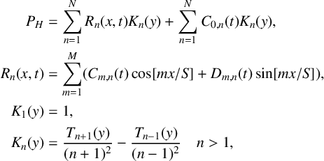 $$ \begin{align*} \begin{aligned} P_H&= \sum_{n=1}^N R_{n}(x,t) K_{n}(y)+\sum_{n=1}^N C_{0,n}(t) K_{n}(y), \\ R_{n}(x,t)&=\sum_{m=1}^M(C_{m,n}(t) \cos[m x/S]+D_{m,n}(t) \sin[m x/S]), \\ K_1(y)&=1, \\ K_n(y)&=\frac{T_{n+1}(y)}{(n+1)^2}-\frac{T_{n-1}(y)}{(n-1)^2} \quad n>1, \end{aligned} \end{align*} $$
where the
 $T_n$
are again the Chebyshev polynomials. The
$T_n$
are again the Chebyshev polynomials. The
 $K_n(y)$
(the Neumann– Chebyshev basis functions) have zero derivatives on
$K_n(y)$
(the Neumann– Chebyshev basis functions) have zero derivatives on
 $y=\pm 1$
, and the inhomogeneous part is met by a field
$y=\pm 1$
, and the inhomogeneous part is met by a field
 $P_I$
, constructed to match the boundary conditions on the walls. In fact, only
$P_I$
, constructed to match the boundary conditions on the walls. In fact, only
 $P_x$
is required, and not P itself, to solve the flow equations, so the single series may safely be ignored unless the pressure itself is desired as an output. To determine the inhomogeneous part
$P_x$
is required, and not P itself, to solve the flow equations, so the single series may safely be ignored unless the pressure itself is desired as an output. To determine the inhomogeneous part
 $P_I$
, we specify
$P_I$
, we specify
 $$ \begin{align*} P_I=\tfrac{1}{4}((y+1)^2 f_2(x)-(y-1)^2 f_1(x)), \end{align*} $$
in which
 $f_1$
and
$f_1$
and
 $f_2$
meet the pressure boundary conditions on
$f_2$
meet the pressure boundary conditions on
 $y=-1$
and
$y=-1$
and
 $y=1$
, respectively. That is, at each time,
$y=1$
, respectively. That is, at each time,
 $$ \begin{align*} f_{1}(x,t)&= - \dfrac{1}{Re} \psi_{xyy}(x,-1,t)-\dfrac{2}{Re}\cos \theta , \\ f_{2}(x,t)&= - \dfrac{1}{Re} \psi_{xyy}(x,1,t)-\dfrac{2}{Re}\cos \theta. \end{align*} $$
The Laplacian of
 $P_I$
and its x-derivative are determined by straightforward differentiation of the basis functions. This allows the isolation of
$P_I$
and its x-derivative are determined by straightforward differentiation of the basis functions. This allows the isolation of
 $\Delta P_H=\Delta P-\Delta P_I$
, and thus the calculation of the coefficients
$\Delta P_H=\Delta P-\Delta P_I$
, and thus the calculation of the coefficients
 $C_{m,n}$
and
$C_{m,n}$
and
 $D_{m,n}$
. Then
$D_{m,n}$
. Then
 $P_x$
is calculated from these coefficients and from
$P_x$
is calculated from these coefficients and from
 $({\partial }/{\partial x})P_I$
.
$({\partial }/{\partial x})P_I$
.
2.7 Integration scheme overview
The overall integration scheme is an explicit RK method consisting of the following calculations at each RK stage.
-
(1) Calculate required spatial variables from the streamfunction coefficients. These are expressed as derivatives of the streamfunction
 $\psi $
.
$\psi $
. -
(2) Solve the vorticity equation to update streamfunction coefficients
$A_{m,n}$
and
$B_{m,n}$
. It was found to be much more stable to use the vorticity equation for this than the momentum equation. -
(3) Solve the PPE for the pressure field P.
-
(4) Solve the momentum equation in the flow direction to compute (∂/∂t)ψ y based on the pressure gradient and gravity forcing. This gives the update to the streamwise velocity coefficients
$A_{0,n}$
.


Thus, to evolve the streamfunction, we consider it to consist of two parts: a “DC” component (the streamwise-averaged part) describing the bulk flow along the channel, and an “AC” component describing the vorticity. The DC component is updated via the momentum equation in the flow direction, and the AC part is updated via the vorticity equation, both given in Table 2.
2.8 Numerical approach
As the governing equations must be solved at each RK step, efficient solution of the governing equations is highly desirable. Accordingly, all variables that are not time dependent are calculated once and cached. The time stepping consists of recreating spatial variables (
 $\psi $
and its derivatives) from the coefficients, solving the two Poisson equations and the momentum equation, and transforming these solutions back into spectral space to update the coefficients.
$\psi $
and its derivatives) from the coefficients, solving the two Poisson equations and the momentum equation, and transforming these solutions back into spectral space to update the coefficients.
The vast majority of the computations may be written in the form of matrix multiplications, the remainder being simple pointwise additions and multiplications. Approximately 90% of processing time is spent on these matrix multiplications. Therefore, efficiency depends almost entirely on an efficient matrix multiplication (“matmul”) routine.
Matrix multiplication is very parallelizable so it is well suited to being solved on a graphical processing unit (GPU). Testing was done with various custom matmul kernels on the GPU, as well as the cuBLAS library and also the Fortran intrinsic “matmul” on the central processing unit. Unsurprisingly, the cuBLAS routines were the fastest, although simple custom cuda kernels were not far behind for small to moderate matrix sizes, especially if they included suitable tiling or fusing of operations.
Note that, for fluid simulations, the use of double precision (64 bit floats) is essential to avoid “round-off” error accumulating and disturbing the results (see Walters and Forbes [Reference Walters and Forbes32] for a comparison of the use of 32 and 64 bit reals in the Rayleigh–Taylor instability). We also note that memory transfers between GPU memory and main memory are very slow compared with the calculations applied to that data, and so they have been entirely avoided within the time-stepping routine. That is, all data is loaded onto the GPU at the start and results are only retrieved when required for plotting. All of the forward integration calculation is processed solely on the GPU, apart from the very small calculation of the truncation error used to adjust the time-step size.
To avoid aliasing issues due to quadratically nonlinear terms in the governing equations, the number of spatial points was set to three times the number of modes, unless otherwise specified. We acknowledge that efficiency may be improved by only using twice as many points as modes and explicitly de-aliasing the nonlinear terms, at the cost of some additional algorithmic complexity. For comparison purposes, the channel was set vertically in all cases (
 $\sin \theta =1, \cos \theta =0$
). In terms of the flow in the channel, this is equivalent to a simple scaling of the gravitational force.
$\sin \theta =1, \cos \theta =0$
). In terms of the flow in the channel, this is equivalent to a simple scaling of the gravitational force.
3 Planar channel–analytic comparison
We now present some exact or analytic solutions for flow in a channel, to confirm that the numerical methods are accurately solving problems according to the governing equations and boundary conditions. This should afford some assurance that the numerical algorithm is correctly set up. For each test, the analytic solution is described, followed by a numerical comparison, and a short discussion. When comparing solutions, the difference considered is simply the greatest absolute difference when the solutions are compared pointwise. All arithmetic is approximated using 64-bit variables throughout this study.
Some simple analytic models are presented for testing the numerical methods and comparisons are shown that validate the numerical algorithm. These solutions include the well-known Poiseuille flow starting from rest, as well as the decay of that flow on removal of the forcing term. This will test the correct calculation of the mean velocity along the channel. To validate the calculation of vorticity, a linearized solution is presented for the lowest eigenmode (two counter-rotating vortices) decaying over time. These two decaying structures (vortices and Poiseuille flow) are superposed and tested. Finally, the full nonlinear numerics are tested by showing that they asymptotically approach the linearized solution over time, as the viscous interaction with the walls becomes dominant. In addition, the energy decay rate is considered and assessed to determine whether the nonlinear behaviour is reasonable.
3.1 Driven Poiseuille flow
The first test is to model flow in a straight-walled channel section, starting from rest and driven by gravity. This should approach the well-known Poiseuille parabolic velocity profile ([Reference Batchelor3, page 183], page 183). For convenience and readability, we let the channel be maximally rotated, with
 $\sin \theta =1$
.
$\sin \theta =1$
.
-
• Analytic solution. We seek a solution of (2.2) but where the flow is in the x-direction only (
$v=0$
), and is independent of x (
$({\partial }/{\partial x})=0$
). In this case, the nondimensionalized momentum equation simplifies to If we assume that
$$ \begin{align*} \frac{\partial u}{\partial t} = \dfrac{1}{Re} \frac{\partial^2 u}{\partial y^2}+ \dfrac{2}{Re}. \end{align*} $$
${\partial u}/{\partial t}=0$
and apply the boundary conditions, we find the steady solution to be Poiseuille flow,
$u_s = 1-y^2$
. The unsteady part may now be found using separations of variables, yielding a series solution for u,
$$ \begin{align*} u & = 1-y^2-\frac{4}{\pi^3}\sum_{n=1}^\infty \frac{\sin[\pi(n-\tfrac{1}{2})(y+1)]\text{Exp }[-\pi^2(n-\tfrac{1}{2})^2 t / Re]}{(n-\tfrac{1}{2})^{3}}. \end{align*} $$
-
• Numerical comparison. The analytic solution is plotted in Figure 1 as dotted lines over the numerical solutions (solid lines). This is shown for four early times
$t=1,2,3,4$
, when acceleration along the centre line is almost constant, and also for times
$10,30,60,200$
to show the development of the flow profile towards the parabolic steady state. It is apparent that the analytic and numerical solutions agree at each time. In fact, they are visually indistinguishable with only 16 modes in each direction, and agree to 64-bit machine precision with number of modes
$\geq 64$
. Reynolds number for this solution is
$Re=100$
. The maximum (dimensionless) velocity along the centre line
$y=0$
approaches
$1$
, as expected. -
• Discussion. The numerical solution is found to agree with the analytic Poiseuille flow. Convergence is rapid, with machine-precision agreement using 64 modes and 320 points in each direction. This confirms that the single-series coefficients
$A_{0,n}$
are correctly calculated through the integration and matrix inversion methods, and that these coefficients are sufficient to describe the streamwise-averaged component of velocity.


Comparison between analytic and numerical solutions for plane Poiseuille flow with
 $Re=100$
. The analytic solution (dotted line), overlays the numerical (solid lines). The solutions at four times are shown in each figure, as marked. The analytic and numerical solutions agree to machine precision for number of modes
$Re=100$
. The analytic solution (dotted line), overlays the numerical (solid lines). The solutions at four times are shown in each figure, as marked. The analytic and numerical solutions agree to machine precision for number of modes
 $\geq 64$
. By time
$\geq 64$
. By time
 $t=200$
, the velocity curve is close to the well-known parabolic profile
$t=200$
, the velocity curve is close to the well-known parabolic profile
 $1-y^2$
with dimensionless speed
$1-y^2$
with dimensionless speed
 $U_c$
in the centre approaching
$U_c$
in the centre approaching
 $1$
.
$1$
.

3.2 Decaying Poiseuille flow
An analytic decaying solution for one-dimensional flow in a channel may also be found, by allowing an established Poiseuille flow to decay on removal of the forcing term.
-
• Analytic solution. Assuming that the flow starts with the steady parabolic profile, and that the forcing term is removed, the velocity profile may be found in the same way as in the previous section to be
The lowest mode decays most slowly, so the initial parabolic profile rapidly approximates the half-period sine wave as it decays to zero.
$$ \begin{align*} u= \frac{4}{\pi^3}\sum_{n=1}^\infty \frac{\sin[\pi(n-\tfrac{1}{2})(y+1)]\text{Exp }[-\pi^2(n-\tfrac{1}{2})^2 t / Re]}{(n-\tfrac{1}{2})^{3}}. \end{align*} $$
-
• Numerical comparison. The results of the numerical and analytic solution are shown in Figure 2, where the two solutions are superposed. Again, the velocity profile across the channel is plotted against the y coordinate. This time, the largest velocity curve corresponds to the initial condition, with times shown near the curves.
-
• Discussion. With only 16 modes and 80 points in each direction, the numerical method using the NSC basis has an error of
$10^{-8}$
. This drops to machine precision on doubling the number of modes and points. It is interesting to note that if we instead use recombined trigonometric functions, the error with 16 modes and 80 points is also of order
$10^{-8}$
, but doubling the number of modes and points only decreases this to
$10^{-9}$
, showing very slow convergence. Note that this is in a system that is decaying to a sinusoidal shape, which explains why the Fourier basis performs even as well as it does here. As mentioned earlier, the Fourier basis cannot properly meet the boundary conditions owing to overly constrained higher derivatives. This is a nice demonstration of the need for a basis that correctly implements boundary conditions.


An initially parabolic Poiseuille profile with forcing removed. The profile decays away, forming a half-period sine profile as it does so. The numerical solution is shown in solid lines with the analytic solution (dots), lying on top of it. The profile rapidly changes from parabolic to sinusoidal.

3.3 Decaying eigenmode behaviour
We now move on to check the accuracy of the numerical solution in solving the vorticity equation. This will test the recovery of the double series coefficients
 $A_{m,n}$
and
$A_{m,n}$
and
 $B_{m,n}$
.
$B_{m,n}$
.
-
• Analytic solution. To provide an analytic solution for comparison, we consider a pair of counter-rotating vortices, obeying the linearized vorticity equation
subject to no-slip boundary conditions in y and periodic boundary conditions in x. We seek a solution of the form
$$ \begin{align*} \frac{\partial \omega}{\partial t}=\frac{1}{Re} \nabla^2 \omega, \end{align*} $$
where
$$ \begin{align*} \psi(x,y,t)=\psi_0(x,y) e^{-\gamma t}, \end{align*} $$
$\psi _0(x,y)$
satisfies the biharmonic eigenvalue problem. The streamfunction
$\psi _0$
is expanded in terms of a Fourier basis in x and a no-slip-compliant basis in y. Using separation of variables and projecting onto the NSC basis leads to a generalized matrix eigenvalue problem. Finding the dominant eigenvalue
$\lambda _1$
of that system using a power iteration yields an initial set of coefficients
$B_n$
such that we have the decaying streamfunction
$$ \begin{align*} \psi=\sum_{n=1}^N[B_n G_n(y)]\sin(x)e^{t/(\lambda_1 Re)}. \end{align*} $$
-
• Numerical comparison. The analytic solution is used to check that the time-stepping method is working correctly. As they use the same basis, the match is accurate to machine precision, so the comparison is not shown here. Instead, as both the decaying vortices and the decaying Poiseuille flow are linear systems, we may superpose them to verify the numerical code when both the vortical components and the DC velocity components are nonzero.
The comparison between analytic and numerical solutions is shown in Figure 3 for times from 0 to 20, with
$Re=100$
. Using 16
$\times $
16 modes, the difference between the two is of order
$10^{-8}$
. At
$32\times 32$
, this difference has dropped to machine precision (
$<10^{-14}$
).Figure 3Comparison between analytic and numerical solutions for an initial condition containing the lowest eigenmode and Poiseuille flow. The velocity component u is shown here, measured at
$x=\pi S/2$
through the centre of the right vortex. The numerical and analytic results are visually identical. The largest amplitude curve is the initial condition (
$t=0$
), and the decayed profile is shown at
$t=5,10,15,20$
, for Reynolds number
$Re=100$
. -
• Discussion. The correct evolution of the velocity coefficients, both for the double series and the single series has been demonstrated here, and provides a check that the components of the numerical method (integrals, time stepping and so on) are functioning correctly. Furthermore, we see that there is no interaction between the two separate modes when the convective terms are ignored, as expected.


3.4 Nonlinear decay
We do not have an analytic solution for the full nonlinear equations. However, we may check for errors by comparing a decaying vortex-pair with the linear solution found above. Over time, we expect that the nonlinear terms will decay more rapidly, with the system approaching the dominant eigenmode from the linear system, as viscosity becomes more important. This is indeed found to be the case, and is seen in Figure 4 where the nonlinear and linearized solutions are shown. Starting from the same initial flow, the linear solution decays as expected (that is, with the same profile at each time). By contrast, the fully nonlinear system “pushes” velocity out towards the walls at
 $y=\pm 1$
, thereby increasing losses. At later times (shown in the panel on the right), as velocities decrease, the viscous term becomes pre-eminent, and the velocity profile approaches the dominant eigenmode of the linear system. Reynolds number was set to
$y=\pm 1$
, thereby increasing losses. At later times (shown in the panel on the right), as velocities decrease, the viscous term becomes pre-eminent, and the velocity profile approaches the dominant eigenmode of the linear system. Reynolds number was set to
 $Re=100$
, and times are shown from
$Re=100$
, and times are shown from
 $0$
up to
$0$
up to
 $19$
.
$19$
.
Linear versus nonlinear decay over time. These are again plots of
 $u(y)$
at
$u(y)$
at
 $x=\pi S/2$
. The dashed lines show the decay of the linearized system, which maintains the single eigenmode profile throughout. The dotted lines show the nonlinear system evolution. The profile changes shape at early times due to the convective terms. As those terms diminish, the viscous term dominates, reasserting the single eigenmode structure. Reynolds number is
$x=\pi S/2$
. The dashed lines show the decay of the linearized system, which maintains the single eigenmode profile throughout. The dotted lines show the nonlinear system evolution. The profile changes shape at early times due to the convective terms. As those terms diminish, the viscous term dominates, reasserting the single eigenmode structure. Reynolds number is
 $Re=100$
, and times are
$Re=100$
, and times are
 $0,3,6,9$
on the left and
$0,3,6,9$
on the left and
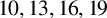 $10,13,16,19$
on the right.
$10,13,16,19$
on the right.

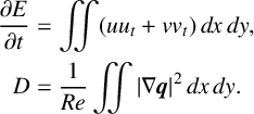
As an additional check, the energy loss and dissipation terms are calculated from the velocities, for both the linearized and nonlinear Navier–Stokes systems as
 $$ \begin{align*} \frac{\partial E}{\partial t}&=\iint (u u_t+v v_t) \, dx\, dy, \\ D&=\frac{1}{Re}\iint |\nabla \boldsymbol q|^2 \, dx \, dy. \end{align*} $$
Then a check of
 $D+({\partial E}/{\partial t})$
is made at each time, and found to be zero, apart from quadrature error (which decreases with grid refinement). This confirms accuracy and consistency in the spectral transforms and time integration. A final check is made by tracking the instantaneous normalized energy decay rate,
$D+({\partial E}/{\partial t})$
is made at each time, and found to be zero, apart from quadrature error (which decreases with grid refinement). This confirms accuracy and consistency in the spectral transforms and time integration. A final check is made by tracking the instantaneous normalized energy decay rate,
 $\gamma _E (t)=-({\partial E}/{\partial t})/E$
, which measures dissipation per unit energy. As expected, this is in constant with the linearized system, being twice the velocity decay constant
$\gamma _E (t)=-({\partial E}/{\partial t})/E$
, which measures dissipation per unit energy. As expected, this is in constant with the linearized system, being twice the velocity decay constant
 $\gamma $
. BY contrast, the nonlinear system decay rate increases rapidly at early times, as the convective terms “push” energy towards the walls, increasing viscous dissipation. The viscous term eventually dominates, returning the decay rate to the predicted linear value. This is shown in Figure 5, with the theoretical prediction and the numerical linear results being identical constants, and the nonlinear result showing expected transient behaviour before relaxing back to the linear profile.
$\gamma $
. BY contrast, the nonlinear system decay rate increases rapidly at early times, as the convective terms “push” energy towards the walls, increasing viscous dissipation. The viscous term eventually dominates, returning the decay rate to the predicted linear value. This is shown in Figure 5, with the theoretical prediction and the numerical linear results being identical constants, and the nonlinear result showing expected transient behaviour before relaxing back to the linear profile.
Linear versus nonlinear energy decay rate over time for
 $Re=100$
. The dashed line shows the theoretical value
$Re=100$
. The dashed line shows the theoretical value
 $2\gamma $
and matches the constant red line showing decay of the linearized system, which maintains the single eigenmode profile throughout. The solid blue line shows the nonlinear system decay rate, which shows a transient surge in early times until settling back to the theoretical value by about time
$2\gamma $
and matches the constant red line showing decay of the linearized system, which maintains the single eigenmode profile throughout. The solid blue line shows the nonlinear system decay rate, which shows a transient surge in early times until settling back to the theoretical value by about time
 $t=80$
.
$t=80$
.

3.5 Validation discussion
We sought out analytic solutions in order to validate the numerical code where possible. We have done this in different regimes: driven Poiseuille flow (testing treatment of body force, boundary conditions and steady-state behaviour); decaying one-dimensional flow (checking temporal accuracy and wall damping effects); dominant eigenmode behaviour (testing spectral accuracy and spectral transform methods); an nonlinear behaviour (checking that the solution approaches the dominant eigenmode in the correct regime, testing energy decay rates).
These tests have applied to the simple geometry where analytic solutions are obtainable. The numerical code may now be applied with some confidence to more irregular geometry, which is described in the next section.
4 Undulating lower boundary–framework
We now consider the more general case of flow in a channel with a periodically structured lower boundary. As above, the channel is inclined at an angle to the gravitational field, but now the lower boundary has profile
 $y=f(x)$
for some function
$y=f(x)$
for some function
 $f(x)$
periodic on
$f(x)$
periodic on
 $-\pi <x<\pi $
. The upper plate is flat and located at
$-\pi <x<\pi $
. The upper plate is flat and located at
 $y = 1$
. To facilitate analysis, the domain is conformally mapped to a rectangular region
$y = 1$
. To facilitate analysis, the domain is conformally mapped to a rectangular region
 $-\pi \leq \xi \leq \pi $
,
$-\pi \leq \xi \leq \pi $
,
 $\eta _0 \leq \eta \leq 1$
, with the value of
$\eta _0 \leq \eta \leq 1$
, with the value of
 $\eta _0$
to be determined. The transformation ensures correct boundary conditions on the sides and top, whereas the lower boundary condition is used to solve for
$\eta _0$
to be determined. The transformation ensures correct boundary conditions on the sides and top, whereas the lower boundary condition is used to solve for
 $\eta _0$
and the mapping coefficients
$\eta _0$
and the mapping coefficients
 $\beta _n$
numerically (described below in Section 4.1).
$\beta _n$
numerically (described below in Section 4.1).
To simplify subsequent computations, the mapped domain is further scaled and translated so that the upper and lower boundaries lie at
 $\eta =\pm 1$
. In consequence, the left and right boundaries are moved to
$\eta =\pm 1$
. In consequence, the left and right boundaries are moved to
 $-S\pi \leq \xi \leq S\pi $
for the required scaling factor S. The computational region now matches that of Section 2, facilitating reuse of the basis functions and coefficient-space transforms used there.
$-S\pi \leq \xi \leq S\pi $
for the required scaling factor S. The computational region now matches that of Section 2, facilitating reuse of the basis functions and coefficient-space transforms used there.
In this section we carefully describe the following: conformal mapping and calculation of metric components; transformation of governing equations into the mapped plane; spectral representation of streamfunction and pressure fields; spectral reconstruction; and implementation details.
4.1 Conformal mapping
To enable the use of simple global basis functions, we map the channel section to a rectangular domain. We choose specifically to make this mapping conformal, as this provides many benefits. These include: preservation of local angles, avoiding artificial anisotropy, and keeping velocity and vorticity fields faithful to the geometry; simplified Laplacian under mapping, reduced number of terms to process in the numerics, particularly in the required Poisson solution; and better spectral efficiency owing to smooth metric coefficients. Conformal mapping is a well-established method for potential flow and linearized Stokes flow problems, but less commonly applied to the full unsteady Navier–Stokes equations.
We thus implement a conformal mapping, based on the requirement that the section of channel must be periodic in x and therefore also in
 $\xi $
. To make the mapping conformal, this requires hyperbolic functions in
$\xi $
. To make the mapping conformal, this requires hyperbolic functions in
 $\eta $
. This Fourier-hyperbolic mapping may be approximated by the finite sum
$\eta $
. This Fourier-hyperbolic mapping may be approximated by the finite sum
 $$ \begin{align} \begin{aligned} x&=\xi/S-\sum_{n=1}^N \beta_n \sin(n \xi/S)\frac{\cosh(n/S(\eta-1))}{\sinh(n(1-\eta_0))},\\ y&=1+\frac{\eta-1}{S}-\sum_{n=1}^N \beta_n \cos(n \xi/S)\frac{\sinh(n/S(\eta-1))}{\sinh(n(1-\eta_0))}, \end{aligned} \end{align} $$
in which
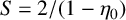 $S=2/(1-\eta _0)$
. The unknown
$S=2/(1-\eta _0)$
. The unknown
 $\eta _0$
and the N coefficients
$\eta _0$
and the N coefficients
 $\beta _n$
are determined using Newton’s method.
$\beta _n$
are determined using Newton’s method.
Figure 6 shows the physical and computational regions, and positioning of grid points, for a chosen boundary
 $y=f(x)$
. Points in
$y=f(x)$
. Points in
 $\xi $
are evenly spaced, whereas points in
$\xi $
are evenly spaced, whereas points in
 $\eta $
are the Chebyshev–Gauss interpolation points (that is, evenly spaced points on a semicircle, projected down onto the plane; specifically,
$\eta $
are the Chebyshev–Gauss interpolation points (that is, evenly spaced points on a semicircle, projected down onto the plane; specifically,
 $\eta (n)=\cos (n-1)\pi /(N-1)$
for
$\eta (n)=\cos (n-1)\pi /(N-1)$
for
 $n=1,\ldots ,N$
). That is, points in the (
$n=1,\ldots ,N$
). That is, points in the (
 $\xi ,\eta $
) grid are placed in exactly the same way as they were for
$\xi ,\eta $
) grid are placed in exactly the same way as they were for
 $x,y$
in the straight channel. For clarity, only 32 by 32 points are shown.
$x,y$
in the straight channel. For clarity, only 32 by 32 points are shown.
Left: the physical space (
 $-\pi <x<\pi ,f(x)<y<1$
) with the lower wall located at
$-\pi <x<\pi ,f(x)<y<1$
) with the lower wall located at
 ${y=f(x)=-5+0.8 \cos x}$
. Right: the mapped computational region (
${y=f(x)=-5+0.8 \cos x}$
. Right: the mapped computational region (
 $\xi ,\eta $
) showing uniform spacing in
$\xi ,\eta $
) showing uniform spacing in
 $\xi $
and Chebyshev spacing in
$\xi $
and Chebyshev spacing in
 $\eta $
(points clustered near the walls).
$\eta $
(points clustered near the walls).

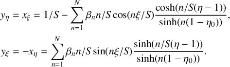
The derivatives of the mapping equations (4.1) will be required in the solution of the flow equations. The derivatives are related by the Cauchy–Riemann equations, so only need to be specified for either x or y. Thus, an immediate benefit of using a conformal map is only having to store half as many terms. We arbitrarily choose the y terms here:
 $$ \begin{align*} y_\eta&=x_\xi=1/S-\sum_{n=1}^N \beta_n n/S \cos(n \xi/S)\frac{\cosh(n/S(\eta-1))}{\sinh(n(1-\eta_0))} ,\\ y_\xi&=-x_\eta=\sum_{n=1}^N \beta_n n/S \sin(n \xi/S)\frac{\sinh(n/S(\eta-1))}{\sinh(n(1-\eta_0))}. \end{align*} $$
Higher derivatives
 $y_{\xi \xi },y_{\eta \eta }$
and so on are derived by straightforward differentiation. Since the mapping (4.1) involves analytic function theory, it follows that x and y and their derivatives satisfy Laplace’s equation in
$y_{\xi \xi },y_{\eta \eta }$
and so on are derived by straightforward differentiation. Since the mapping (4.1) involves analytic function theory, it follows that x and y and their derivatives satisfy Laplace’s equation in
 $\xi $
and
$\xi $
and
 $\eta $
. These arrays do not change over time, so may be computed once and cached in memory for use throughout the numerical routine.
$\eta $
. These arrays do not change over time, so may be computed once and cached in memory for use throughout the numerical routine.
4.2 Flow equations in the mapped domain
The governing equations must now be transformed to the computational (
 $\xi ,\eta $
) plane, to allow solution in a geometry that enables the use of the efficient spectral methods used in the previous section. This will add many terms to the vorticity, momentum and pressure equations. However, the orthogonality of the conformal mapping greatly simplifies and reduces the number of terms required. In addition, we are still able to use the streamfunction formulation, implicitly satisfying the incompressibility condition.
$\xi ,\eta $
) plane, to allow solution in a geometry that enables the use of the efficient spectral methods used in the previous section. This will add many terms to the vorticity, momentum and pressure equations. However, the orthogonality of the conformal mapping greatly simplifies and reduces the number of terms required. In addition, we are still able to use the streamfunction formulation, implicitly satisfying the incompressibility condition.
In this section, we describe the coordinate transform and associated identities. Then the four transformed flow equations are described (continuity, vorticity, pressure, momentum). A summary of these equations is provided at the end.
4.2.1 Coordinate transform and identities
Starting with the velocity vector
 $\boldsymbol q=u \boldsymbol i + v \boldsymbol j$
in Cartesian coordinates, its components in the
$\boldsymbol q=u \boldsymbol i + v \boldsymbol j$
in Cartesian coordinates, its components in the
 $(\xi ,\eta )$
plane are written
$(\xi ,\eta )$
plane are written
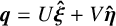 $\boldsymbol q=U \boldsymbol {\hat \xi } + V \boldsymbol {\hat \eta }$
, where the new coordinate unit vectors are
$\boldsymbol q=U \boldsymbol {\hat \xi } + V \boldsymbol {\hat \eta }$
, where the new coordinate unit vectors are
 $$ \begin{align*} \boldsymbol{\hat\xi}&=\frac{x_\xi \boldsymbol i+y_\xi \boldsymbol j}{\sqrt{x_\xi^2+y_\xi^2}}, \quad \boldsymbol{\hat\eta}=\frac{x_\eta \boldsymbol i+y_\eta \boldsymbol j}{\sqrt{x_\eta^2+y_\eta^2}}. \end{align*} $$
Because the mapping is conformal, the Cauchy–Riemann equations hold, so
 ${x_\xi =y_\eta }$
and
${x_\xi =y_\eta }$
and
 $x_\eta =-y_\xi $
. Thus the metric conversion may be described using only two of these. As already mentioned, in this paper we will use
$x_\eta =-y_\xi $
. Thus the metric conversion may be described using only two of these. As already mentioned, in this paper we will use
 $y_\eta $
and
$y_\eta $
and
 $y_\xi $
. For readability, we introduce
$y_\xi $
. For readability, we introduce
 $\kappa (\xi ,\eta )=(x_\xi ^2+y_\xi ^2)^{-1}=(x_\eta ^2+y_\eta ^2)^{-1}=(y_\xi ^2+y_\eta ^2)^{-1}$
. Note that, due to conformality,
$\kappa (\xi ,\eta )=(x_\xi ^2+y_\xi ^2)^{-1}=(x_\eta ^2+y_\eta ^2)^{-1}=(y_\xi ^2+y_\eta ^2)^{-1}$
. Note that, due to conformality,
 $\xi _y=\kappa y_\xi $
and
$\xi _y=\kappa y_\xi $
and
 $\eta _y=\kappa y_\eta $
. Therefore the conversion of velocity components is written as
$\eta _y=\kappa y_\eta $
. Therefore the conversion of velocity components is written as
 $$ \begin{align*} u&=\kappa^{1/2}(y_\eta U-y_\xi V),\\ v&=\kappa^{1/2}(y_\xi U+y_\eta V). \end{align*} $$
In this paper capitalized
 $U,V$
always refer to the velocity components in the mapped (
$U,V$
always refer to the velocity components in the mapped (
 $\xi ,\eta $
) space, whereas lower case
$\xi ,\eta $
) space, whereas lower case
 $u,v$
are the standard components in physical (
$u,v$
are the standard components in physical (
 $x,y$
) space. As we are now working in (
$x,y$
) space. As we are now working in (
 $\xi ,\eta $
) space, we designate
$\xi ,\eta $
) space, we designate
 $\nabla _{x,y}$
to be the grad operator in physical space and
$\nabla _{x,y}$
to be the grad operator in physical space and
 $\Delta _{x,y}$
to mean
$\Delta _{x,y}$
to mean
 $\partial _{xx}+\partial _{yy}$
, and we redefine
$\partial _{xx}+\partial _{yy}$
, and we redefine
 $\nabla \equiv (\partial _\xi ,\partial _\eta )$
and
$\nabla \equiv (\partial _\xi ,\partial _\eta )$
and
 $\Delta \equiv \partial _{\xi \xi }+\partial _{\eta \eta }$
. The scalar Laplacian operator under the conformal mapping has the identity
$\Delta \equiv \partial _{\xi \xi }+\partial _{\eta \eta }$
. The scalar Laplacian operator under the conformal mapping has the identity
 $$ \begin{align*} \Delta_{x,y} =\kappa \Delta. \end{align*} $$
The time-independent metric term
 $\kappa $
and its required derivatives may be calculated using straightforward differentiation and cached at the start of the numerical routine, from the conformal mapping
$\kappa $
and its required derivatives may be calculated using straightforward differentiation and cached at the start of the numerical routine, from the conformal mapping
 $$ \begin{align*} \kappa&=(y_\xi^2+y_\eta^2)^{-1},\\ \kappa_\xi&=-2\kappa^2(y_\xi y_{\xi\xi}+y_\eta y_{\xi\eta}),\\ \kappa_\eta&=-2\kappa^2(y_\xi y_{\xi\eta}-y_\eta y_{\xi\xi}),\\ \kappa_{\xi\xi}&=2\kappa_\xi^2/\kappa-2\kappa^2(y_{\xi\xi}^2+y_{\xi\eta}^2+y_\eta y_{\xi\xi\eta}+y_\xi y_{\xi\xi\xi}),\\ \Delta \kappa&=4\kappa^2(y_{\xi\xi}^2+y_{\xi\eta}^2). \end{align*} $$
These are all the derivatives of
 $\kappa $
required for the numerical method.
$\kappa $
required for the numerical method.
4.2.2 Continuity equation
Under the conformal mapping, the continuity equation
 $\boldsymbol {\nabla }_{x,y} \cdot \mathbf {q}=\mathbf {0}$
can be shown to be
$\boldsymbol {\nabla }_{x,y} \cdot \mathbf {q}=\mathbf {0}$
can be shown to be
 $$ \begin{align*} & \frac{\partial}{\partial \xi}\bigg(\frac{U}{\kappa^{1/2}}\bigg)+\frac{\partial}{\partial \eta}\bigg(\frac{V}{\kappa^{1/2}}\bigg)=0, \end{align*} $$
allowing U and V to be written in terms of a streamfunction as
 $$ \begin{align*} U & =\kappa^{1/2}\frac{\partial\psi}{\partial\eta}, \quad V=-\kappa^{1/2}\frac{\partial\psi}{\partial\xi}. \end{align*} $$
As in the straight-channel case, continuity may be satisfied through the use of a streamfunction.
4.2.3 Vorticity equation
The vorticity
 $\omega =-\Delta _{x,y} \psi $
is evolved via (2.3), which we rewrite here as
$\omega =-\Delta _{x,y} \psi $
is evolved via (2.3), which we rewrite here as
 $$ \begin{align*} \omega_t & =\dfrac{1}{Re} \Delta_{x,y} \omega - (u \omega_x+v \omega_y). \end{align*} $$
The conversions for the components of the vorticity equation are found to be
 $$ \begin{align*} u&=\kappa(y_{\eta}\psi_{\eta}+y_{\xi}\psi_{\xi}),\\ v&=\kappa(y_{\xi}\psi_{\eta}-y_{\eta}\psi_{\xi}),\\ \omega&=-\kappa \Delta \psi , \\ \omega_x&=\kappa(y_\xi \kappa_\eta-y_\eta \kappa_\xi) \Delta \psi +\kappa^2 (y_\xi \Delta \psi_\eta-y_\eta \Delta \psi_\xi),\\ \omega_y&=-\kappa(y_\xi \kappa_\xi+y_\eta \kappa_\eta) \Delta \psi -\kappa^2(y_{\xi}\Delta \psi_\xi+y_{\eta}\Delta \psi_\eta),\\ \Delta_{x,y}\omega&=-\kappa^2 \Delta^2 \psi-2\kappa^2(\kappa_\xi \Delta \psi_\xi+\kappa_\eta \Delta \psi_\eta)-\kappa \Delta \psi \Delta \kappa. \end{align*} $$
Using these formulations for vorticity and its derivatives in terms of
 $\psi $
, the mapped vorticity equation, although initially very complicated, simplifies significantly to
$\psi $
, the mapped vorticity equation, although initially very complicated, simplifies significantly to
 $$ \begin{align*} \Delta \psi_t&=\dfrac{1}{Re}(\kappa\Delta^2 \psi+2(\kappa_\xi \Delta \psi_\xi+\kappa_\eta \Delta \psi_\eta) + \Delta \psi \Delta \kappa) \\ &\quad+\Delta \psi(\kappa_\eta \psi_\xi-\kappa_\xi \psi_\eta)+\kappa(\psi_\xi \Delta \psi_\eta-\psi_\eta \Delta \psi_\xi). \end{align*} $$
This is now in a form analogous to Section 2, and is amenable to solution using the same spectral integration method.
4.2.4 PPE
Incorporating the incompressibility condition, the PPE is
 $$ \begin{align*} \Delta_{x,y} P & = - 2 (u_x^2+u_y v_x). \end{align*} $$
Applying the chain rule to these velocity derivatives and the scalar Laplacian, we can write
 $$ \begin{align*} \Delta P&= - \frac{2}{\kappa}(u_x^2+u_y v_x) \\ &= - 2\kappa[(y_\eta u_\xi-y_\xi u_\eta)^2+(y_\xi u_\xi+y_\eta u_\eta) (y_\eta v_\xi-y_\xi v_\eta)] \\ &= 2\kappa(\psi_{\xi\xi} \psi_{\eta\eta}-\psi_{\xi\eta}^2)-\dfrac{1}{2}(\psi_{\xi}^2+\psi_{\eta}^2)\Delta \kappa \\ &\quad+(\kappa_\eta \psi_\eta-\kappa_\xi \psi_\xi)(\psi_{\xi\xi} - \psi_{\eta\eta})-2 \psi_{\xi\eta}(\kappa_\xi \psi_\eta + \kappa_\eta \psi_\xi), \end{align*} $$
which is a suitable form for efficient computation using the methods from Section 2.
The pressure boundary conditions must also be transformed into (
 $\xi ,\eta $
) space. The no-slip boundaries imply that
$\xi ,\eta $
) space. The no-slip boundaries imply that
 $\psi _\eta $
and
$\psi _\eta $
and
 $\psi _\xi $
are both zero on the boundaries
$\psi _\xi $
are both zero on the boundaries
 $\eta =\pm 1$
, as are all of their
$\eta =\pm 1$
, as are all of their
 $\xi $
-derivatives, allowing the mapped form of the pressure boundary conditions to be written as
$\xi $
-derivatives, allowing the mapped form of the pressure boundary conditions to be written as
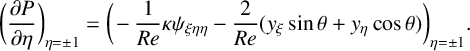 $$ \begin{align*} \bigg(\frac{\partial P}{\partial \eta}\bigg )_{\eta=\pm1} & =\bigg(\!-\dfrac{1}{Re} \kappa \psi_{\xi\eta\eta}- \dfrac{2}{Re}(y_\xi \sin \theta + y_\eta \cos \theta)\bigg )_{\eta=\pm1}. \end{align*} $$
Thus the pressure again has Neumann boundary conditions. To represent pressure using global basis functions while enforcing these boundary conditions, we again split pressure into a part with homogeneous boundaries and an inhomogeneous part, that is,
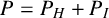 $P=P_H+P_I$
, as for the straight channel. This is directly analogous to what was done in Section 2, but now includes some additional terms due to the mapping. So, we define the inhomogeneous part via boundary conditions, denoted
$P=P_H+P_I$
, as for the straight channel. This is directly analogous to what was done in Section 2, but now includes some additional terms due to the mapping. So, we define the inhomogeneous part via boundary conditions, denoted
 $f_1(\xi )$
and
$f_1(\xi )$
and
 $f_2(\xi )$
, as
$f_2(\xi )$
, as
 $$ \begin{align*} P_I&=\dfrac{1}{4}[(\eta+1)^2 f_2(\xi)-(\eta-1)^2 f_1(\xi)],\\ f_{1,2}(\xi)&=\bigg(\!-\frac{1}{Re} \kappa \psi_{\xi\eta\eta}- \frac{2}{Re}(y_\xi \sin \theta + y_\eta \cos \theta)\bigg )_{\eta=-1,1}, \end{align*} $$
so that
 $\partial P_I/\partial \eta $
is equal to
$\partial P_I/\partial \eta $
is equal to
 $f_1$
on
$f_1$
on
 $\eta =-1$
and
$\eta =-1$
and
 $f_2$
on
$f_2$
on
 $\eta =1$
. The derivatives of
$\eta =1$
. The derivatives of
 $f_1$
and
$f_1$
and
 $f_2$
are required to calculate
$f_2$
are required to calculate
 $\partial P_I/\partial \xi $
for the momentum equation, and also to calculate the Laplacian of
$\partial P_I/\partial \xi $
for the momentum equation, and also to calculate the Laplacian of
 $P_I$
for solving the PPE itself.
$P_I$
for solving the PPE itself.
 $$ \begin{align*} f^{\prime}_{1,2}(\xi)&=\bigg(\!-\frac{1}{Re} (\kappa_\xi \psi_{\xi\eta\eta}+\kappa \psi_{\xi\xi\eta\eta})-\frac{2}{Re}(y_{\xi\xi} \sin \theta+y_{\xi\eta} \cos \theta)\bigg)_{\eta=-1,1}, \\ f^{\prime\prime}_{1,2}(\xi)&=\bigg(\!-\frac{1}{Re} (\kappa_{\xi\xi} \psi_{\xi\eta\eta}+2\kappa_\xi \psi_{\xi\xi\eta\eta}+\kappa \psi_{\xi\xi\xi\eta\eta}) -\frac{2}{Re}(y_{\xi\xi\xi} \sin \theta + y_{\xi\xi\eta} \cos \theta)\bigg)_{\eta=-1,1}. \end{align*} $$
4.2.5
$\xi $
-Momentum equation

It remains to present the
 $\xi $
-momentum equation in the (
$\xi $
-momentum equation in the (
 $\xi ,\eta $
) domain. The conversion yields
$\xi ,\eta $
) domain. The conversion yields
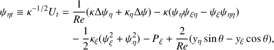 $$ \begin{align*} \psi_{\eta t} \equiv \kappa^{-1/2} U_t & =\frac{1}{Re}(\kappa \Delta \psi_\eta+\kappa_\eta \Delta \psi)-\kappa(\psi_\eta \psi_{\xi\eta}-\psi_\xi \psi_{\eta\eta})\\ &\quad - \dfrac{1}{2}\kappa_\xi(\psi_\xi^2+\psi_\eta^2)-P_\xi+\frac{2}{Re}(y_\eta \sin \theta - y_\xi \cos \theta ), \end{align*} $$
in which the total pressure gradient is constructed from both homogeneous and inhomogeneous parts, that is
 $P_\xi =({\partial }/{\partial \xi })(P_I)+({\partial }/{\partial \xi })(P_H)$
.
$P_\xi =({\partial }/{\partial \xi })(P_I)+({\partial }/{\partial \xi })(P_H)$
.
4.2.6 Summary of governing equations
As a simple check, it may be shown that, for a trivial mapping of a rectangular region back to itself, we have
 $x_\xi =y_\eta =1$
and
$x_\xi =y_\eta =1$
and
 $x_\eta =y_\xi =0$
, and so
$x_\eta =y_\xi =0$
, and so
 $\kappa =1$
,
$\kappa =1$
,
 $\kappa _\xi =\kappa _\eta =0$
,
$\kappa _\xi =\kappa _\eta =0$
,
 $U=u$
and
$U=u$
and
 $V=v$
, recovering the standard equations for a straight channel, as summarized in Table 2. The summary of the conformally mapped equations to be solved is shown in Table 3.
$V=v$
, recovering the standard equations for a straight channel, as summarized in Table 2. The summary of the conformally mapped equations to be solved is shown in Table 3.
Summary of governing equations and boundary conditions for the wavy channel. Subscripts indicate spatial or temporal derivatives.

As for the straight-channel case, the flow may again be solved by evolution in time by solving two Poisson equations and the momentum equation in the
 $\xi $
direction, subject to their boundary conditions. We are now ready to proceed with the numerical strategy, basis functions and integration methods.
$\xi $
direction, subject to their boundary conditions. We are now ready to proceed with the numerical strategy, basis functions and integration methods.
4.3 Basis functions
The computational approach is now described in terms of basis functions for the velocity streamfunction and for pressure, test functions, time-integration scheme and spectral calculations. This follows closely the approach given for the straight channel, so will be described in brief.
The velocity streamfunction is represented using the same NSC basis that was used in the straight-walled channel, Section 2: that is,
 $$ \begin{align*} \psi(\xi,\eta,t) &= \sum_{n=1}^N F_{n}(\xi,t) G_n(\eta)+A_{0,n} H_n(\eta), \end{align*} $$
in which we define the functions in exact analogy to those in the straight-walled channel, Section 2,
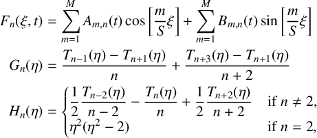 $$ \begin{align*} F_{n}(\xi,t)&=\sum_{m=1}^{M} A_{m,n}(t) \cos\bigg[\frac{m}{S} \xi\bigg]+\sum_{m=1}^{M} B_{m,n}(t) \sin\bigg[\frac{m}{S} \xi\bigg]&&\nonumber\\G_n(\eta) &= \frac{T_{n-1}(\eta)-T_{n+1}(\eta)}{n} + \frac{T_{n+3}(\eta)-T_{n+1}(\eta)}{n+2}&&\nonumber\\H_n(\eta) &=\begin{cases}\displaystyle\frac{1}{2} \dfrac{T_{n-2}(\eta)}{n-2} - \dfrac{T_n(\eta)}{n} + \displaystyle\frac{1}{2} \dfrac{T_{n+2}(\eta)}{n+2} \quad\text{if } n \neq 2, \nonumber\\ \eta^2(\eta^2 - 2) \qquad\qquad\qquad\ \ \ \,\qquad\ \hspace{0.4pt} \text{if } n = 2, \nonumber\end{cases} \end{align*} $$
so that
 $H_n'(\eta )=T_{n+1}(\eta )-T_{n-1}(\eta )$
are the appropriate Neumann–Chebyshev functions for the uniform flow.
$H_n'(\eta )=T_{n+1}(\eta )-T_{n-1}(\eta )$
are the appropriate Neumann–Chebyshev functions for the uniform flow.
Also in direct analogy with the straight-channel analysis, pressure has inhomogeneous boundary conditions, so it is split into an inhomogeneous part and a homogeneous part:
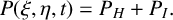 $$ \begin{align*} P(\xi,\eta,t) =P_H+P_I. \end{align*} $$
The homogeneous part may now be described using the same homogeneous Neumann basis functions, but in terms of (
 $\xi ,\eta $
) as
$\xi ,\eta $
) as
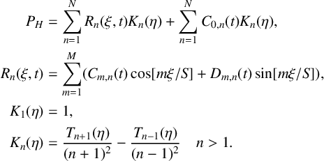 $$ \begin{align*} \begin{aligned} P_H&= \sum_{n=1}^N R_{n}(\xi,t) K_{n}(\eta)+\sum_{n=1}^N C_{0,n}(t) K_{n}(\eta),\\ R_{n}(\xi,t)&=\sum_{m=1}^M(C_{m,n}(t) \cos[m \xi/S]+D_{m,n}(t) \sin[m \xi/S]),\\ K_1(\eta)&=1 ,\\ K_n(\eta)&=\frac{T_{n+1}(\eta)}{(n+1)^2}-\frac{T_{n-1}(\eta)}{(n-1)^2} \quad n>1. \end{aligned} \end{align*} $$
4.4 Time-integration scheme
The exact same explicit RK method is used as described for the straight channel. That is, we create spatial variables from the streamfunction coefficients, and solve the Poisson equations for vorticity and pressure, and the streamwise momentum equation. Then we update the streamfunction coefficients
 $A_{m,n}$
,
$A_{m,n}$
,
 $A_{0,n}$
and
$A_{0,n}$
and
 $B_{m,n}$
at each full time step of the RK method.
$B_{m,n}$
at each full time step of the RK method.
4.5 Numerical approach
The numerical approach is identical to the straight-channel model, except for four subroutines, which are those that return the right-hand side values for the vorticity, pressure and momentum equations, and the pressure boundary functions
 $f_1, f_2$
and their derivatives. These four functions compute the left-hand side of the equations shown in Table 3. As before, the majority of the required computational load is in performing matrix multiplications on the GPU.
$f_1, f_2$
and their derivatives. These four functions compute the left-hand side of the equations shown in Table 3. As before, the majority of the required computational load is in performing matrix multiplications on the GPU.
5 Undulating wall–semianalytic comparison
In the case of a channel with an undulating wall, it is difficult to find analytic results for comparison. There has, however, been a significant amount of work in the field of lubrication theory for a channel of slowly varying width. We follow the approach of Tavakol et al. [Reference Tavakol, Froehlicher, Holmes and Stone28] to estimate the pressure drop due to the undulating wall. With the full height of our channel being
 $H(x)=2-\epsilon \cos (x)$
, we have the leading-order term
$H(x)=2-\epsilon \cos (x)$
, we have the leading-order term
 $$ \begin{align*} \Delta P_0=\frac{3}{\pi}\int_{-\pi}^\pi H^{-3}\, dx. \end{align*} $$
Using residue theory, this was evaluated to
 $$ \begin{align*} \Delta P_0=3 \frac{8+\epsilon^2}{(4-\epsilon^2)^{5/2}}. \end{align*} $$
The corresponding flux through the channel in our model is then given by
 $Q=1/\Delta P_0$
. The effect of these wall perturbations on the fluid flux along the channel is measured and compared with standard Poiseuille flow. The flux here is defined as the integral of the streamwise velocity component along a vertical line from wall to wall. That is, for bottom wall profile
$Q=1/\Delta P_0$
. The effect of these wall perturbations on the fluid flux along the channel is measured and compared with standard Poiseuille flow. The flux here is defined as the integral of the streamwise velocity component along a vertical line from wall to wall. That is, for bottom wall profile
 $y=f(x)$
,
$y=f(x)$
,
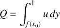 $$ \begin{align*} Q=\int_{f(x_0)}^1 u \, dy \end{align*} $$
for any vertical line
 $x=x_0$
. For the Poiseuille flow in our nondimensional units, with
$x=x_0$
. For the Poiseuille flow in our nondimensional units, with
 $u=1-y^2$
(that is, with
$u=1-y^2$
(that is, with
 $f(x)=-1$
), this yields
$f(x)=-1$
), this yields
 $Q=4/3$
. On conversion to the (
$Q=4/3$
. On conversion to the (
 $\xi ,\eta $
) coordinates, the flux may be expressed as
$\xi ,\eta $
) coordinates, the flux may be expressed as
 $$ \begin{align*} Q=\int_{-1}^1 \frac{\partial \psi}{\partial \eta} \, d \eta = \psi(\xi_0,1)-\psi(\xi_0,-1) \end{align*} $$
for any chosen line
 $\xi =\xi _0$
, corresponding to normal flux through a curve that joins top and bottom walls.
$\xi =\xi _0$
, corresponding to normal flux through a curve that joins top and bottom walls.
Another approach to approximate the flow is to formally linearize the system, based on the small parameter
 $\epsilon $
, the wall perturbation. We approximate the velocities and the pressure for the Stokes flow equations as
$\epsilon $
, the wall perturbation. We approximate the velocities and the pressure for the Stokes flow equations as
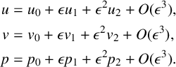 $$ \begin{align*} u&=u_0+\epsilon u_1+\epsilon^2 u_2+O(\epsilon^3),\\ v&=v_0+\epsilon v_1+\epsilon^2 v_2+O(\epsilon^3),\\ p&=p_0+\epsilon p_1+\epsilon^2 p_2+O(\epsilon^3). \end{align*} $$
Using these to expand the Stokes flow equations
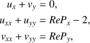 $$ \begin{align*} u_x+v_y&=0,\\ u_{xx}+u_{yy}&=Re P_x - 2,\\ v_{xx}+v_{yy}&=Re P_y, \end{align*} $$
we find
 $u_0=1-y^2$
,
$u_0=1-y^2$
,
 $v_0=0$
and
$v_0=0$
and
 $P_0=0$
(that is, Poiseuille flow). At the next order, projecting the lower boundary conditions onto
$P_0=0$
(that is, Poiseuille flow). At the next order, projecting the lower boundary conditions onto
 $y=-1$
using Taylor series, we find
$y=-1$
using Taylor series, we find
 $$ \begin{align*} u_1&=\cos(x) F(y),\\ v_1&=\sin(x) G(y),\\ p_1&=\sin(x) S(y), \end{align*} $$
where
 $$ \begin{align*} F(y)=(A+B y)\mathrm{e}^y+(C+D y)\mathrm{e}^{-y}, \end{align*} $$
and
 $G'=F$
. The constants
$G'=F$
. The constants
 $A, B, C, D$
are determined from the boundary conditions to be
$A, B, C, D$
are determined from the boundary conditions to be
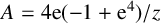 $A=4 \mathrm {e} (-1+\mathrm {e}^4)/z$
,
$A=4 \mathrm {e} (-1+\mathrm {e}^4)/z$
,
 $B=-2 \mathrm {e} (1+3\mathrm {e}^4)/z$
,
$B=-2 \mathrm {e} (1+3\mathrm {e}^4)/z$
,
 $C=16 \mathrm {e}^3/z$
and
$C=16 \mathrm {e}^3/z$
and
 $D=2 \mathrm {e}^3 (-5+\mathrm {e}^4)/z$
, in which
$D=2 \mathrm {e}^3 (-5+\mathrm {e}^4)/z$
, in which
 $z=(1-18 \mathrm {e}^4+\mathrm {e}^8)$
.
$z=(1-18 \mathrm {e}^4+\mathrm {e}^8)$
.
It turns out that
 $\int _{-1}^1 F(y) \, dy=0$
, so there is no contribution to bulk flux at first order. Following a similar process to second order, we find that there is a contribution, so that bulk flow is
$\int _{-1}^1 F(y) \, dy=0$
, so there is no contribution to bulk flux at first order. Following a similar process to second order, we find that there is a contribution, so that bulk flow is
 $$ \begin{align*} \begin{aligned} Q&=Q_0+\epsilon^2 Q_2+O(\epsilon^3), \\ Q&=4/3+\epsilon^2 \bigg(\frac{5+14 \mathrm{e}^4-3 \mathrm{e}^8}{2-36 \mathrm{e}^4+2 \mathrm{e}^8}+\dfrac{1}{2} \bigg)+O(\epsilon^3). \end{aligned} \end{align*} $$
This flux is shown in Figure 7, along with the leading-order lubrication theory and the numerical results, where a low Reynolds number (
 $Re=1$
) was used to keep the flow laminar and vortex free. In addition, to match the analytic approximations (for Stokes flow), the nonlinear terms in the vorticity and momentum equation were set to zero. We see that, for small
$Re=1$
) was used to keep the flow laminar and vortex free. In addition, to match the analytic approximations (for Stokes flow), the nonlinear terms in the vorticity and momentum equation were set to zero. We see that, for small
 $\epsilon $
, the approximations are very close to the numerical results, with the perturbation expansion visually indistinguishable up to about
$\epsilon $
, the approximations are very close to the numerical results, with the perturbation expansion visually indistinguishable up to about
 $\epsilon =0.2$
. The linearization becomes less accurate for larger
$\epsilon =0.2$
. The linearization becomes less accurate for larger
 $\epsilon $
, as expected. We have found that this approximation may be made more accurate as higher-order terms in
$\epsilon $
, as expected. We have found that this approximation may be made more accurate as higher-order terms in
 $\epsilon $
are included. The lubrication theory is a reasonably good approximation for large
$\epsilon $
are included. The lubrication theory is a reasonably good approximation for large
 $\epsilon $
, as it uses the full lower-wall function, linearizing with just the aspect ratio of the channel rather than the boundary parameter
$\epsilon $
, as it uses the full lower-wall function, linearizing with just the aspect ratio of the channel rather than the boundary parameter
 $\epsilon $
itself. Overall, these results are consistent with the numerical model being close to the true solution.
$\epsilon $
itself. Overall, these results are consistent with the numerical model being close to the true solution.
Flux for laminar flow through the channel at various amplitudes of the lower-wall function, from
 $\epsilon =0$
to
$\epsilon =0$
to
 $\epsilon =1$
. The simulation is shown with a solid line, the second-order linearization correction is shown with a dashed line and the leading-order lubrication approximation is a dashed–dotted line.
$\epsilon =1$
. The simulation is shown with a solid line, the second-order linearization correction is shown with a dashed line and the leading-order lubrication approximation is a dashed–dotted line.

6 Numerical results
Some sample computational results are now presented for various wall shapes. We begin with some less demanding channel shapes and low Reynolds number flows. We first consider the evolution of the flow with smooth wall shapes. We define an effective flux as
 $$ \begin{align*} Q_{\text{eff}}=\frac{Q}{Q_0}, \end{align*} $$
where Q is the flux and
 $Q_0=4/3$
is the flux for pure Poiseuille flow. This gives bulk flow through the channel relative to developed straight-channel flow for a channel
$Q_0=4/3$
is the flux for pure Poiseuille flow. This gives bulk flow through the channel relative to developed straight-channel flow for a channel
 $-1<y<1$
. The evolution of fluid flow over a large trough is shown in Figure 8. Three distinct stages may be observed. Vortex-free flow exists up until
$-1<y<1$
. The evolution of fluid flow over a large trough is shown in Figure 8. Three distinct stages may be observed. Vortex-free flow exists up until
 $t=80$
, when a vortex forms on the upwind side of the trough, at
$t=80$
, when a vortex forms on the upwind side of the trough, at
 $x\approx -0.9$
, with an effective flux of
$x\approx -0.9$
, with an effective flux of
 $Q_{\text {eff}}\approx 0.15$
. This single vortex slowly stretches until it fills the trough by about
$Q_{\text {eff}}\approx 0.15$
. This single vortex slowly stretches until it fills the trough by about
 $t=700$
, with
$t=700$
, with
 $Q_{\text {eff}}\approx 0.52$
. By
$Q_{\text {eff}}\approx 0.52$
. By
 $t=720$
, the vortex is oscillating, and by
$t=720$
, the vortex is oscillating, and by
 $t=800$
has split in two, the vortices “rolling along” the trough, forming on the upstream side and dissipating on the downstream side. This limits the flow to about
$t=800$
has split in two, the vortices “rolling along” the trough, forming on the upstream side and dissipating on the downstream side. This limits the flow to about
 $Q_{\text {eff}}=0.54$
, forming a quasisteady state. For clarity, only the lower half of the channel is shown, and the contour lines have been weighted to show more detail near the lower wall.
$Q_{\text {eff}}=0.54$
, forming a quasisteady state. For clarity, only the lower half of the channel is shown, and the contour lines have been weighted to show more detail near the lower wall.
The evolution of the vortex structure in a sinusoidal trough with nominal
 $Re=1200$
is shown in the four plots. The background colour indicates local fluid speed. Plots are shown for times 80, 700, 720 and 800, from top to bottom.
$Re=1200$
is shown in the four plots. The background colour indicates local fluid speed. Plots are shown for times 80, 700, 720 and 800, from top to bottom.

In a similar layout, the time evolution of fluid flow over a large asymmetric bump is shown in Figure 9, with nominal Reynolds number
 $Re=1200$
, at times 100, 600, 720 and 1200. The early flow is seen in the top frame, where a vortex has just formed on the trailing edge. The second frame shows a large vortex filling the trough between the (periodic) bumps. Again, this oscillates and forms the creation absorption cycle (third frame), but with largely horizontal flow in the upper part of the channel. This is the time of fastest flow. The fourth frame shows that the vortices are interacting strongly with the main flow, pulling high-speed fluid close to the walls. This results in loss of energy to the walls, reducing the bulk flux through the channel. Effective flux
$Re=1200$
, at times 100, 600, 720 and 1200. The early flow is seen in the top frame, where a vortex has just formed on the trailing edge. The second frame shows a large vortex filling the trough between the (periodic) bumps. Again, this oscillates and forms the creation absorption cycle (third frame), but with largely horizontal flow in the upper part of the channel. This is the time of fastest flow. The fourth frame shows that the vortices are interacting strongly with the main flow, pulling high-speed fluid close to the walls. This results in loss of energy to the walls, reducing the bulk flux through the channel. Effective flux
 $Q_{\text {eff}}$
from top to bottom is 0.14, 0.52, 0.71 and 0.26, showing a dramatic loss of energy once a large vortex interacts strongly with the flow. This is shown in Figure 10, where the square root of kinetic energy, integrated over the domain, is plotted against time.
$Q_{\text {eff}}$
from top to bottom is 0.14, 0.52, 0.71 and 0.26, showing a dramatic loss of energy once a large vortex interacts strongly with the flow. This is shown in Figure 10, where the square root of kinetic energy, integrated over the domain, is plotted against time.
The evolution of the vortex structure between asymmetric bumps with nominal
 $Re=1200$
is shown in the four plots, with the dimensionless time t shown in each frame. Again, the background colour indicates local fluid speed.
$Re=1200$
is shown in the four plots, with the dimensionless time t shown in each frame. Again, the background colour indicates local fluid speed.
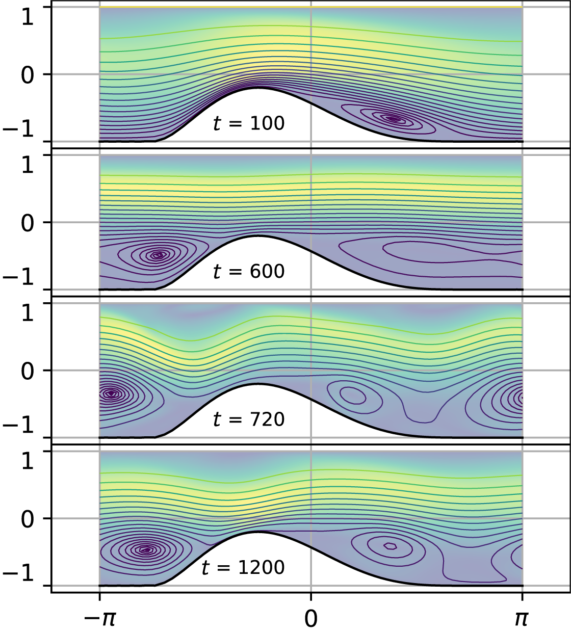
Energy–time plot for the simulation of Figure 9, showing a large drop in kinetic energy caused by vortices directing fast moving fluid near to the lower wall. The wiggles in the energy represent formation and detachment of vortices near the wavy wall.

Flow over a narrow trough is presented in Figure 11, for nominal
 $Re=2000$
. A vortex forms in the trough, with horizontal flow above. Once the fluid is moving fast enough to drag the vortex out of the trough, it interferes with the main flow, drawing faster fluid close to the wall and reducing the bulk flow through the channel. This reduction is seen in the energy–time plot in Figure 12. Effective flux
$Re=2000$
. A vortex forms in the trough, with horizontal flow above. Once the fluid is moving fast enough to drag the vortex out of the trough, it interferes with the main flow, drawing faster fluid close to the wall and reducing the bulk flow through the channel. This reduction is seen in the energy–time plot in Figure 12. Effective flux
 $Q_{\mathrm{eff}}$
from top to bottom is 0.08, 0.15, 0.43 and 0.66.
$Q_{\mathrm{eff}}$
from top to bottom is 0.08, 0.15, 0.43 and 0.66.
Flow over a narrow trough with nominal
 $Re=2000$
is shown in the four plots. Again, the background colour indicates local fluid speed. Times from top to bottom are 60, 120, 480 and 2000. Once the vortex is interacting strongly with the main flow, the bulk flow through the channel is reduced, as seen in the reduction in energy in Figure 12.
$Re=2000$
is shown in the four plots. Again, the background colour indicates local fluid speed. Times from top to bottom are 60, 120, 480 and 2000. Once the vortex is interacting strongly with the main flow, the bulk flow through the channel is reduced, as seen in the reduction in energy in Figure 12.

Energy–time plot for the simulation of Figure 11, showing a drop in kinetic energy caused by vortices interacting with the main flow, and again directing fast moving fluid into the lower-wall boundary layer.
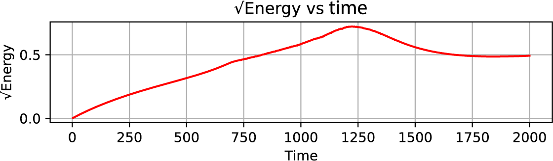
We now test convergence of the method for a more demanding simulation, high Reynolds number flow over an undulating wall. This is an opportunity to determine the performance of the scheme where higher accuracy is demanded. We consider flow with nominal Reynolds number
 $Re=10^5$
, in a channel
$Re=10^5$
, in a channel
 $-\pi <x<\pi,\ f(x)<y<1 $
,
$-\pi <x<\pi,\ f(x)<y<1 $
,
 $f(x)=-1-0.1 \cos x$
. At high flow rates, the vortex shedding becomes moderately periodic, and we track the total kinetic energy in Figure 13.
$f(x)=-1-0.1 \cos x$
. At high flow rates, the vortex shedding becomes moderately periodic, and we track the total kinetic energy in Figure 13.
The total kinetic energy for nominal
 $Re=10^5$
is shown for increasing grid fineness from top to bottom. The top plot is for the coarsest grid,
$Re=10^5$
is shown for increasing grid fineness from top to bottom. The top plot is for the coarsest grid,
 $M=N=16$
, with three points per mode. The second plot has twice that number of modes and points in each direction and the bottom plot has five times as many. The fluctuations are not of numerical origin, but rather correspond to the effects of vortex formation at the lower wall.
$M=N=16$
, with three points per mode. The second plot has twice that number of modes and points in each direction and the bottom plot has five times as many. The fluctuations are not of numerical origin, but rather correspond to the effects of vortex formation at the lower wall.

To get some statistically meaningful comparisons, these runs were continued out to
 $t=10^6$
, and the results are shown in Table 4. Designating a precision level p, such that number of modes in each direction is
$t=10^6$
, and the results are shown in Table 4. Designating a precision level p, such that number of modes in each direction is
 $16p$
, the time-averaged kinetic energy increases from 0.023 to about 0.039 as p increases, plateauing by
$16p$
, the time-averaged kinetic energy increases from 0.023 to about 0.039 as p increases, plateauing by
 $p=3\text {--}4$
, suggesting statistical convergence. The standard deviation (std) also increases up to
$p=3\text {--}4$
, suggesting statistical convergence. The standard deviation (std) also increases up to
 $p=4$
and then plateaus, which is consistent with converged unsteady behaviour. The integral timescale (
$p=4$
and then plateaus, which is consistent with converged unsteady behaviour. The integral timescale (
 $\tau \approx 1.1\times 10^4$
–
$\tau \approx 1.1\times 10^4$
–
 $1.9 \times 10^4$
) indicates a consistent dominant unsteady timescale across precision levels. By extending the run up to
$1.9 \times 10^4$
) indicates a consistent dominant unsteady timescale across precision levels. By extending the run up to
 $t=10^6$
, we obtained effective sample sizes
$t=10^6$
, we obtained effective sample sizes
 $N_{\mathrm {eff}} \approx 26$
–
$N_{\mathrm {eff}} \approx 26$
–
 $47$
, ensuring a statistically meaningful estimate of the mean. The standard error of the mean (SEM) is consistently less than
$47$
, ensuring a statistically meaningful estimate of the mean. The standard error of the mean (SEM) is consistently less than
 $2\%$
of the mean, indicating that the mean kinetic energy is statistically stable. The actual time series are plotted in Figure 13. Based on this data, it is fair to say that the flow has converged to within sampling uncertainty by
$2\%$
of the mean, indicating that the mean kinetic energy is statistically stable. The actual time series are plotted in Figure 13. Based on this data, it is fair to say that the flow has converged to within sampling uncertainty by
 $p=4$
, with 64 modes and 192 points in each dimension.
$p=4$
, with 64 modes and 192 points in each dimension.
Summary statistics for the kinetic energy time series at each precision level p. Mean and std are computed over the statistically stationary portion of the flow. The integral time scale
 $\tau $
and effective sample size
$\tau $
and effective sample size
 $N_{\mathrm {eff}}$
are derived from the autocorrelation function. The SEM is also shown.
$N_{\mathrm {eff}}$
are derived from the autocorrelation function. The SEM is also shown.

Some benchmarking is now provided for higher Reynolds number flow, including runtimes and number of basic operations, to allow comparison with other methods. Counting the average number of operations at each RK stage, for a method with S stages with number of modes M and N, and points
 $N_x$
and
$N_x$
and
 $N_y$
, we find the number of floating point operations (FLOPs) to be
$N_y$
, we find the number of floating point operations (FLOPs) to be
 $$ \begin{align*} FLOPs&=3(S-1)(MN+N/2)+28 M N_x N+34 N_x N N_y +6 M N_y \\ &\quad+106 N_xN_y+45N_x+2NN_y+4N^2N_x+8MN^2 +8N_xN. \end{align*} $$
The
 $S-1$
term may seem strange, but it is due to the calculation of the next evaluation point, which takes a number of additions dependent on all the RK stages before it. To simplify, consider the case where
$S-1$
term may seem strange, but it is due to the calculation of the next evaluation point, which takes a number of additions dependent on all the RK stages before it. To simplify, consider the case where
 $M=N$
and
$M=N$
and
 $N_x=N_y=3M$
, and with
$N_x=N_y=3M$
, and with
 $S=16$
(the 8/9 tableau), this is
$S=16$
(the 8/9 tableau), this is
 $$ \begin{align*} \text{FLOPs}=410N^3+1025N^2+157.5N. \end{align*} $$
Total FLOPs can then be counted by multiplying FLOPs per stage by number of stages by total number of loops. We then divide by wall-clock time for all the loops to get a throughput. This is shown in
 $10^9$
operations per second in Table 5, where timing data, throughput and memory usage are shown for the runs used in the convergence tests in Figure 13, with precision levels p from 1 to 5 and
$10^9$
operations per second in Table 5, where timing data, throughput and memory usage are shown for the runs used in the convergence tests in Figure 13, with precision levels p from 1 to 5 and
 $Re=10^5$
, and where the flow is simulated up to
$Re=10^5$
, and where the flow is simulated up to
 $t=10^6$
. All the adaptive RK simulations in this paper were adjusted via a local relative tolerance of
$t=10^6$
. All the adaptive RK simulations in this paper were adjusted via a local relative tolerance of
 $reltol=10^{-5}$
and an absolute tolerance of
$reltol=10^{-5}$
and an absolute tolerance of
 $abstol=10^{-9}$
, with a global error control target of
$abstol=10^{-9}$
, with a global error control target of
 $rktol=10^{-7}$
. Step size was adjusted to keep the root-mean-square of the normalized local errors less than
$rktol=10^{-7}$
. Step size was adjusted to keep the root-mean-square of the normalized local errors less than
 $rktol$
.
$rktol$
.
Timing, throughput and GPU memory usage data for the runs used in Table 4.
 $Re=10^5$
and the simulations were run up to
$Re=10^5$
and the simulations were run up to
 $t=10^6$
.
$t=10^6$
.

Considering only the
 $410 N^3$
operations and ignoring
$410 N^3$
operations and ignoring
 $O(N)$
and
$O(N)$
and
 $O(N^2)$
operations, the breakdown is
$O(N^2)$
operations, the breakdown is
 $34 N^3$
for retrieving the pressure coefficients
$34 N^3$
for retrieving the pressure coefficients
 $C_{m,n}, D_{m,n}$
,
$C_{m,n}, D_{m,n}$
,
 $18 N^3$
for the single-series coefficients
$18 N^3$
for the single-series coefficients
 $d/dt(A_{0,n})$
,
$d/dt(A_{0,n})$
,
 $34 N^3$
for the vorticity coefficients
$34 N^3$
for the vorticity coefficients
 $d/dt(A_{m,n}), d/dt(B_{m,n})$
, and the remaining
$d/dt(A_{m,n}), d/dt(B_{m,n})$
, and the remaining
 $324 N^3$
operations for creating all the spatial variables from the coefficients. Although
$324 N^3$
operations for creating all the spatial variables from the coefficients. Although
 $O(N^3)$
matrix multiplies have been used for simplicity and ease of parallelization, the use of fast Fourier transforms may significantly reduce runtimes, ideally from
$O(N^3)$
matrix multiplies have been used for simplicity and ease of parallelization, the use of fast Fourier transforms may significantly reduce runtimes, ideally from
 $O(N^3)$
to
$O(N^3)$
to
 $O(N^2 \log (N))$
.
$O(N^2 \log (N))$
.
Theoretical maximum throughput for the GP100 card used is
 $5100$
GFLOPS. For the relatively small matrix sizes used, memory fetches dominate, especially at the smallest sizes. Thus, even though the number of operations scales as
$5100$
GFLOPS. For the relatively small matrix sizes used, memory fetches dominate, especially at the smallest sizes. Thus, even though the number of operations scales as
 $N^3$
, the runtime is scaling much more slowly for small N. It would be surprising if there are not significant further efficiency improvements that could be pursued, but that is beyond the scope of this paper. A more modern GPU with larger memory caches is also expected to perform better.
$N^3$
, the runtime is scaling much more slowly for small N. It would be surprising if there are not significant further efficiency improvements that could be pursued, but that is beyond the scope of this paper. A more modern GPU with larger memory caches is also expected to perform better.
The memory usage appears to follow the expected quadratic scaling, with a fixed overhead of 257 MiB and array usage of
 $\sim 1.36 p^2$
MiB. These two-dimensional arrays are small, relative to the 16GB of GPU memory available, even for
$\sim 1.36 p^2$
MiB. These two-dimensional arrays are small, relative to the 16GB of GPU memory available, even for
 $p=5$
. A value of
$p=5$
. A value of
 $p=100$
(1600 modes in each direction) would fit, although runtime at these tolerances would be infeasibly large. This indicates that GPU memory usage is not likely to be a constraining issue if this method is adapted to three-dimensional flows.
$p=100$
(1600 modes in each direction) would fit, although runtime at these tolerances would be infeasibly large. This indicates that GPU memory usage is not likely to be a constraining issue if this method is adapted to three-dimensional flows.
Finally, we present the performance of five different RK methods for the
 $Re=10^5$
case for a run up to
$Re=10^5$
case for a run up to
 $t=10^4$
. The methods are a third-order (second-order embedded) “bs23” due to Bogacki and Shampine [Reference Bogacki and Shampine4], three fifth-order (fourth-order embedded) Fehlberg’s [Reference Fehlberg11]‘rkf45’, Dormand and Prince’s [Reference Dormand and Prince10] “dopri5”, and Bogacki and Shampine’s “bs45(8)” (based on [Reference Bogacki and Shampine5] with an added eighth stage, coefficients found on Peter Stone’s site [Reference Stone25]) and Verner’s [Reference Verner30] “most robust” sixteen-stage ninth-order, eighth-order embedded method “v89”.
$t=10^4$
. The methods are a third-order (second-order embedded) “bs23” due to Bogacki and Shampine [Reference Bogacki and Shampine4], three fifth-order (fourth-order embedded) Fehlberg’s [Reference Fehlberg11]‘rkf45’, Dormand and Prince’s [Reference Dormand and Prince10] “dopri5”, and Bogacki and Shampine’s “bs45(8)” (based on [Reference Bogacki and Shampine5] with an added eighth stage, coefficients found on Peter Stone’s site [Reference Stone25]) and Verner’s [Reference Verner30] “most robust” sixteen-stage ninth-order, eighth-order embedded method “v89”.
The results for the five RK methods are shown in Table 6. As well as the time to complete the run, we have shown the number of effective stages (the Bogacki–Shampine methods and the Dormand–Prince method have the first-same-as-last property, so they effectively use one fewer stage than their tableaux suggest. At high
 $Re$
, with the tight tolerances used, the third-order method (bs23) was very slow. The three fifth-order methods were much faster, with dopri5 slightly faster than rkf45, and the bs45(8) method being more than twice as fast as rkf45 (we often find this to be the case, at least with smooth fluid flow; the bs45(8) has been tuned for very low truncation error). Verner’s 9(8) method was almost twice as fast again, suggesting that it may be worth trying even higher-order methods. These results highlight that our streamfunction/PPE approach benefits fully from high-order RK integrators, achieving the expected speedups from reduced step counts without the complications of pressure–velocity splitting. In the interests of caution, we note that the timing comparisons are quite different for lower Reynolds number flows. We have included runs at
$Re$
, with the tight tolerances used, the third-order method (bs23) was very slow. The three fifth-order methods were much faster, with dopri5 slightly faster than rkf45, and the bs45(8) method being more than twice as fast as rkf45 (we often find this to be the case, at least with smooth fluid flow; the bs45(8) has been tuned for very low truncation error). Verner’s 9(8) method was almost twice as fast again, suggesting that it may be worth trying even higher-order methods. These results highlight that our streamfunction/PPE approach benefits fully from high-order RK integrators, achieving the expected speedups from reduced step counts without the complications of pressure–velocity splitting. In the interests of caution, we note that the timing comparisons are quite different for lower Reynolds number flows. We have included runs at
 $Re=1000$
and
$Re=1000$
and
 $Re=100$
for comparison. These were run up to
$Re=100$
for comparison. These were run up to
 $t=Re/10$
. For
$t=Re/10$
. For
 $Re=1000$
, all methods gave similar timings, except the ninth-order, which took twice as long. For
$Re=1000$
, all methods gave similar timings, except the ninth-order, which took twice as long. For
 $Re=100$
, neither the bs45(8) nor Verner’s 9(8) method finished in a reasonable time.
$Re=100$
, neither the bs45(8) nor Verner’s 9(8) method finished in a reasonable time.
Performance of different RK methods. The simulation for Table 4 was run for various values of Reynolds number, up to
 $t=Re/10$
, and timed using five different RK methods. “Effective stages” takes into account the models that have the first-same-as-last property. Entries with “dnf” indicate that the run did not finish within a time at least
$t=Re/10$
, and timed using five different RK methods. “Effective stages” takes into account the models that have the first-same-as-last property. Entries with “dnf” indicate that the run did not finish within a time at least
 $10\times $
as large as the next slowest time. Times are in seconds.
$10\times $
as large as the next slowest time. Times are in seconds.
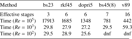
7 Conclusions
We have presented a novel approach to modelling flow in a channel with one undulating wall. It represents a synthesis of established techniques—streamfunction formulation, global spectral approach, numerical conformal mapping and high-order explicit time integration—combined in a new way that gives a clean, efficient and accurate way to model such flows. The accuracy of the method has been evaluated against several analytic or semianalytic solutions, and found to be good, even with a small number of points and modes.
The streamfunction formulation ensures that continuity is satisfied by construction, eliminating the need for iterative pressure–velocity coupling. The PPE is relegated to auxiliary status, and solved directly at each RK stage, with boundary conditions imposed exactly via basis functions.
The approach in this paper therefore facilitates the effective use of high-order explicit time-stepping methods. The numerical analysis shows that at higher Reynolds number and for tight error tolerances (
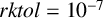 $rktol=10^{-7}$
), our method benefits strongly from higher-order RK methods, with use of a ninth-order method achieving approximate
$rktol=10^{-7}$
), our method benefits strongly from higher-order RK methods, with use of a ninth-order method achieving approximate
 $2\text {--}4 \times $
speedup when compared with fifth-order methods (depending on the particular fifth-order method used), with even larger gains (
$2\text {--}4 \times $
speedup when compared with fifth-order methods (depending on the particular fifth-order method used), with even larger gains (
 $40 \times $
) observed relative to the third-order method. The PPE solution at each RK stage accounts for approximately
$40 \times $
) observed relative to the third-order method. The PPE solution at each RK stage accounts for approximately
 $8\%$
of the dominant computational operations, with the majority of the cost being construction of the spatial variables. This ratio is expected to hold if matrix multiplications are replaced by fast Fourier transform operations, as such optimization would apply uniformly to all such multiplications in the RK loop.
$8\%$
of the dominant computational operations, with the majority of the cost being construction of the spatial variables. This ratio is expected to hold if matrix multiplications are replaced by fast Fourier transform operations, as such optimization would apply uniformly to all such multiplications in the RK loop.
For regions with smooth boundaries, this method gives a good alternative to finite-difference and finite-element methods. No difficulty is anticipated in adapting the conformal mapping to the case where both walls are smooth functions of x. Future areas of research include adapting to more difficult geometries and three-dimensional domains, which may require the use of a quasiconformal mapping based on solutions of the three-dimensional Laplace equation. In addition, parametrization of the wall shape should allow the use of walls with overturning structures, not just functions of x. Optimization of the numerical routines could include replacement of matrix multiplications with fast Fourier transform operations, more efficient anti-aliasing, use of higher-order integrators and consideration of nonexplicit solvers. In addition, if only the steady-state solution is required, rather than the full evolution from rest, other iterative methods may be considered.
The method presented in this study combines the exponential accuracy of a spectral approach, the speed of higher-order RK methods, the explicit treatment of the PPE as an auxiliary equation with direct solve using correct boundary conditions and a numerical conformal mapping. The result is an elegant and straightforward algorithm for modelling two-dimensional flow in a smooth periodic channel with undulating walls.

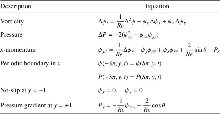
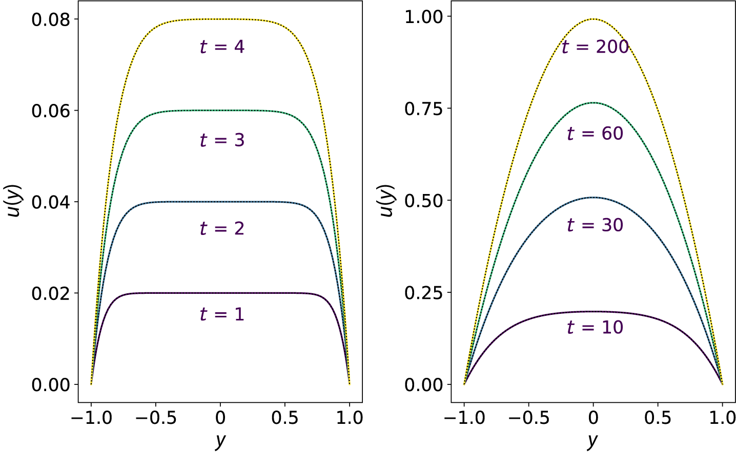


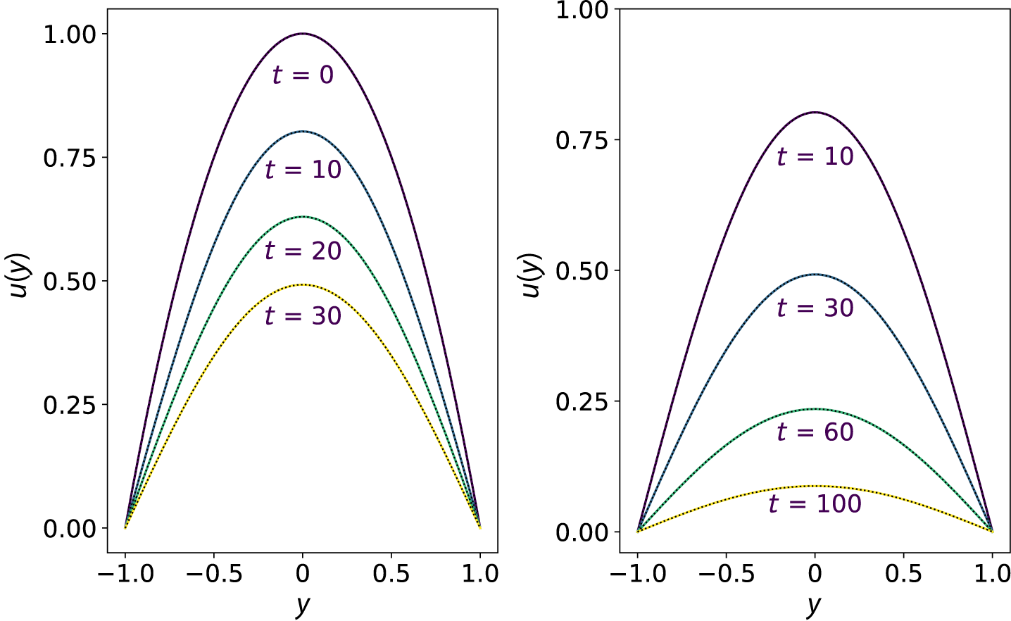
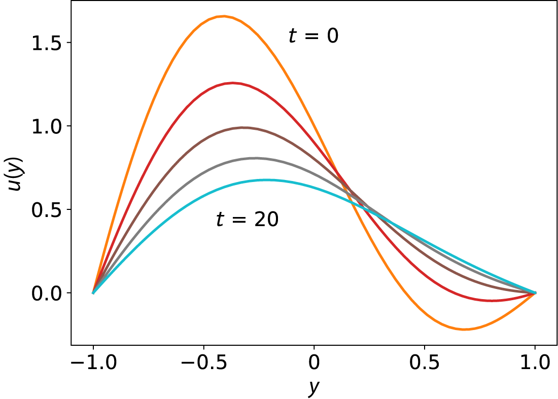


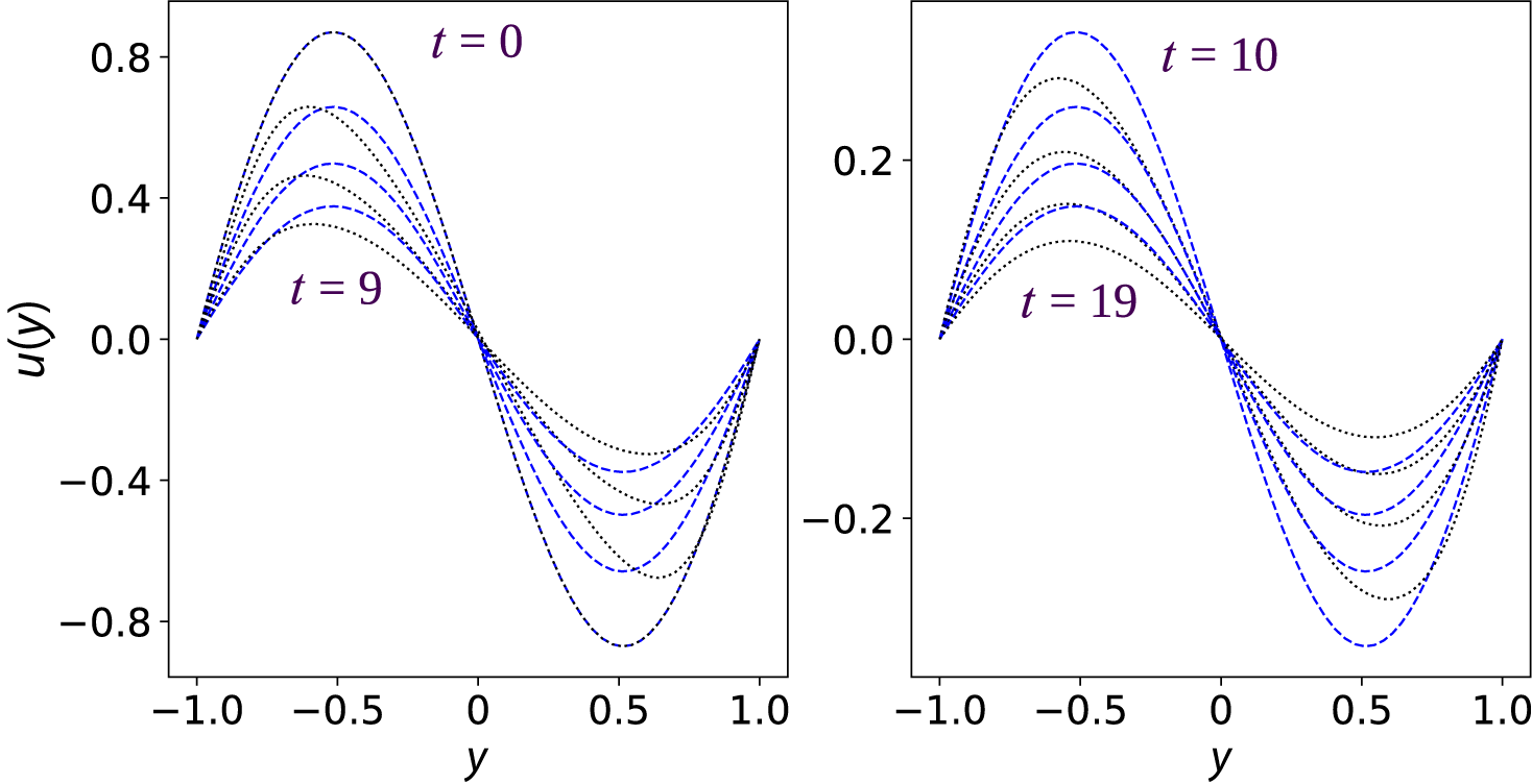


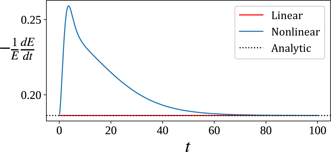


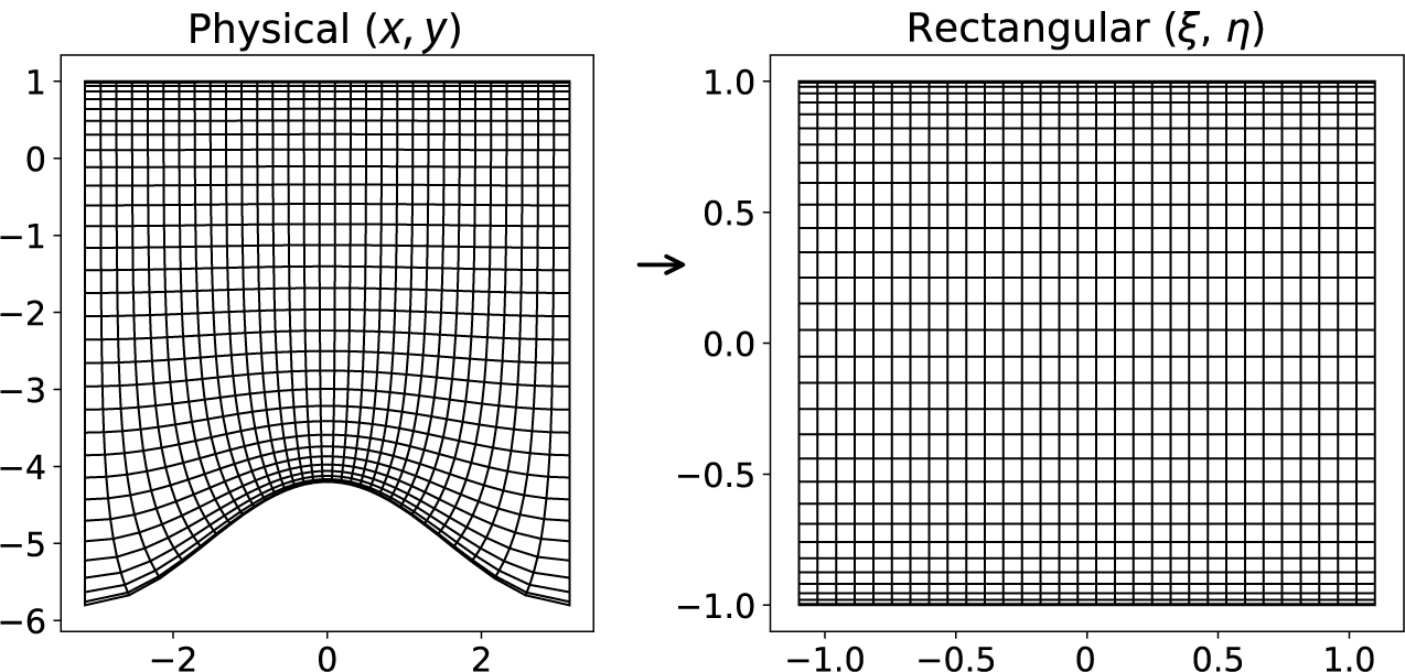


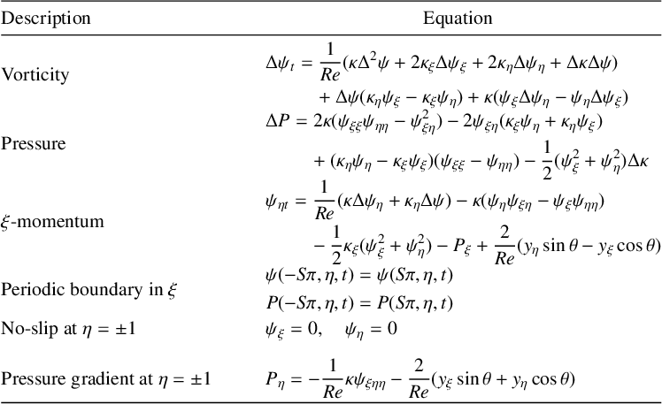
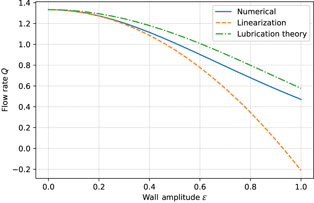


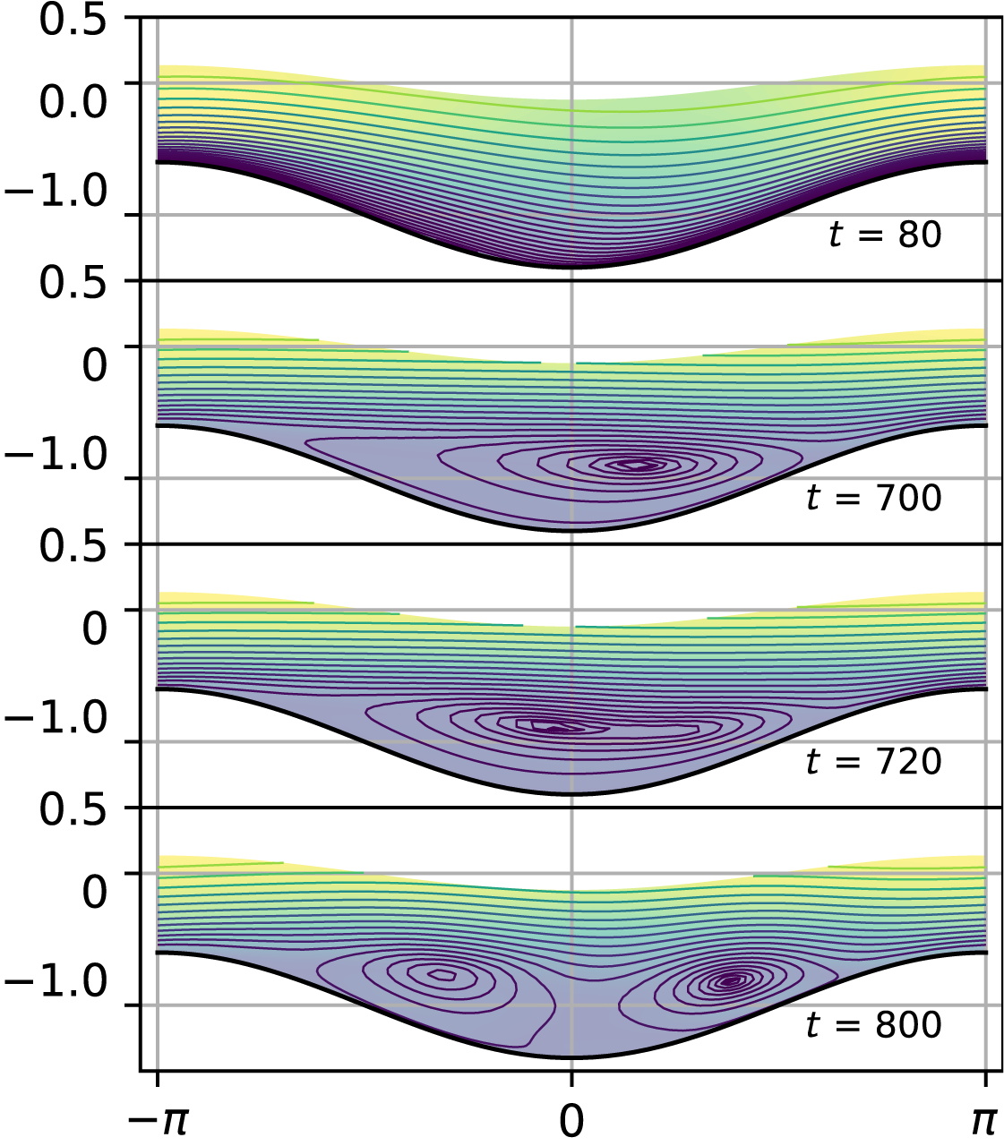


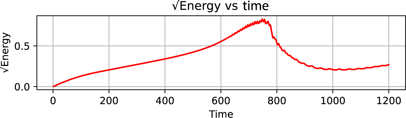
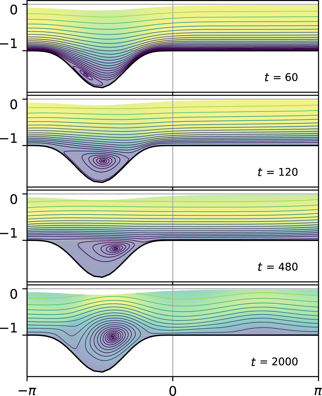


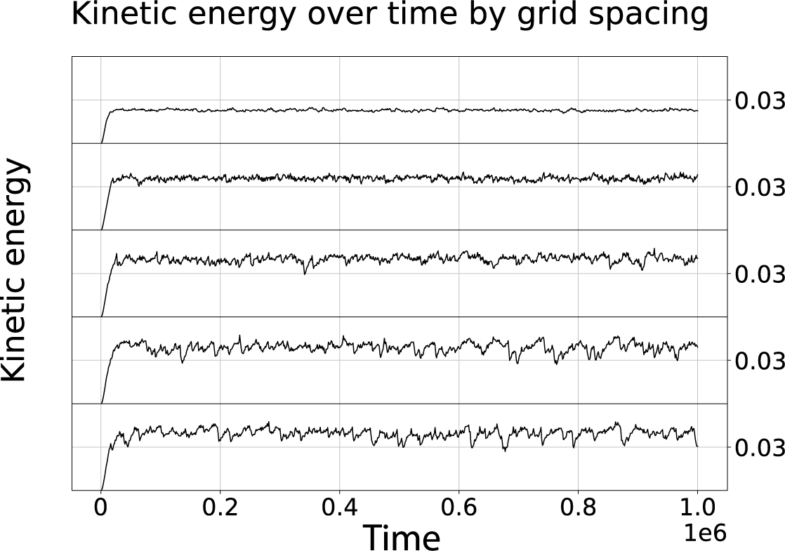


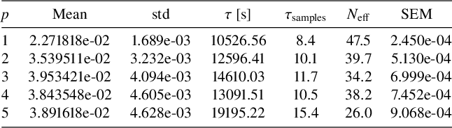


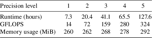


 Open access