

1. INTRODUCTION
Mountain glaciers worldwide have retreated significantly in the past decades as a consequence of an increase in global temperature (Vaughan and others, Reference Vaughan and Stocker2013). This resulted in an important contribution to global sea-level rise (Church and others, Reference Church and Stocker2013; Marzeion and others, Reference Marzeion2017) and profoundly affects water supply, hydro-electricity production, natural hazards and tourism in mountainous regions (e.g. Werder and others, Reference Werder, Bauder, Funk and Keusen2010; Farinotti and others, Reference Farinotti, Usselmann, Huss, Bauder and Funk2012; Vincent and others, Reference Vincent2012; Gilbert and others, Reference Gilbert, Vincent, Gagliardini, Krug and Berthier2015; Huss and Hock, Reference Huss and Hock2015, Reference Huss and Hock2018; Ragettli and others, Reference Ragettli, Immerzeel and Pellicciotti2016; Kääb and others, Reference Klok and Oerlemans2018). Many studies have highlighted these changes for glaciers in the Swiss Alps through a wide range of approaches, based on for instance geodetic methods, LIDAR measurements, Unmanned Aerial Vehicle (UAV) surveys and three-dimensional glacier evolution modelling (Jouvet and others, Reference Jouvet, Huss, Blatter, Picasso and Rappaz2009; Gabbud and others, Reference Gabbud, Micheletti and Lane2015, Reference Gabbud, Micheletti and Lane2016; Zekollari and Huybrechts, Reference Zekollari and Huybrechts2015; Fischer and others, Reference Fischer, Huss, Kummert and Hoelzle2016; Sold and others, Reference Sold2016; Gindraux and others, Reference Gindraux, Boesch and Farinotti2017; Rossini and others, Reference Réveillet, Vincent, Six and Rabatel2018). These changes are largely driven by a strongly negative surface mass-balance (SMB) trend (Huss and others, Reference Huss, Dhulst and Bauder2015; Zemp and others, Reference Zemp2015; Vincent and others, Reference Vincent and Vallon2017), which has been modelled at a variety of horizontal scales and through models of varying complexity for glaciers in the European Alps (e.g. Klok and Oerlemans, Reference Klok and Oerlemans2002; Huss and others, Reference Huss, Bauder, Funk and Hock2008; Machguth and others, Reference Machguth, Paul, Kotlarski and Hoelzle2009; Nemec and others, Reference Nemec, Huybrechts, Rybak and Oerlemans2009; Berthier and Vincent, Reference Berthier and Vincent2012; Gabbi and others, Reference Gabbi, Carenzo, Pellicciotti, Bauder and Funk2014; Huss and Fischer, Reference Huss and Fischer2016; Réveillet and others, Reference Rossini2017). Process-based SMB models are powerful and very useful tools for many applications, but they rely on parameterisations, simplifications and assumptions that influence the relationship between the model input (meteorological data) and output (modelled SMB). In order to better quantify the link between meteorological data and SMB, direct statistical methods therefore represent an attractive alternative. Furthermore, such statistical methods can be useful tools for cases where the necessary measurements needed to setup more sophisticated SMB models (e.g. albedo and radiation measurements) are not available.
The first studies that laid the foundation for multivariate statistical regression between SMB data and meteorological observations were performed at the end of the 1970s (Young, Reference Young1977; Martin, Reference Martin1978; Tangborn, Reference Tangborn1980). Since then, multivariate statistical regressions have been widely applied, under slightly varying forms, among others for glaciers in the Rocky Mountains and Coast Mountains (Western Canada) (Letréguilly, Reference Letréguilly1988), Svalbard (Lefauconnier and Hagen, Reference Lefauconnier and Hagen1990; Lefauconnier and others, Reference Lefauconnier, Hagen, Ørbæk, Melvold and Isaksson1999), Norway (e.g. Trachsel and Nesje, Reference Trachsel and Nesje2015) and in the European Alps (e.g. Chen and Funk, Reference Chen and Funk1990; Vincent and Vallon, Reference Vincent1997; Torinesi and others, Reference Torinesi, Letréguilly and Valla2002). The majority of these studies highlight the importance of summer temperature and winter precipitation, which variables are typically used to describe the observed SMB trends.
Here we analyse a 15-year dataset of SMB measurements from the ablation zone of the Morteratsch glacier complex (Switzerland) and investigate the meteorological variables that best describe the interannual variability in SMB through multiple linear regression analysis (MLRA). Compared with previous studies, where the meteorological input mostly consists of adjacent clusters of months, we introduce a new method in which all possible monthly combinations are considered. Our main objective is to make use of this new method to describe the measured SMB variations through a statistical analysis that is as simple as possible, i.e. relying on a minimal number of predictor variables to describe as much of the SMB variability as possible.
2. LOCATION, FIELDWORK AND DATA
2.1. Location and fieldwork
The Morteratsch glacier complex is situated on the southern side of the European Alps (Engadine, SE Switzerland) and consists of two glaciers, the Morteratsch glacier (Vadret da Morteratsch) and the Pers glacier (Vadret Pers) (Fig. 1). Until 2015, Vadret Pers was the main tributary of the Vadret da Morteratsch (Zekollari and Huybrechts, Reference Zekollari and Huybrechts2015), but now both glaciers have disconnected and act as independent ice bodies. At present, the glacier complex covers an area of ~16 km2 and has a volume of ~1.1 km3 (Zekollari and others, Reference Zekollari, Huybrechts, Fürst, Rybak and Eisen2013).
Overview of the Morteratsch glacier complex and stakes for SMB measurements in the ablation area. The eight stakes used in the multiple linear regression analysis (MLRA) are shown in blue (Vadret da Morteratsch) and red (Vadret Pers), the other stakes are represented in light grey. The terminus is at ~2100 m a.s.l., while the highest mountain peaks are ~4000 m. The SwissTopo Digital Elevation Model (DEM) used to produce this figure is from 2001 (i.e. start of the field campaign). Figure created with TopoZeko toolbox (Zekollari, Reference Zekollari2017).

Since 2001 we measured the SMB on the glacier complex from an elaborate stake network emplaced in its ablation area and around the ELA. These measurements were performed at the very end of September/beginning of October, around the time of the first snowfall events that mark the end of the ablation season and the onset of the accumulation season. For some years, some additional ablation occurred in October, while for others the annual ice ablation already stopped at the time of measurements due to an earlier (September) snowfall event. The stake position was measured with high precision GPS systems, which were corrected with reference base stations until 2013 (see Zekollari and others, Reference Zekollari, Huybrechts, Fürst, Rybak and Eisen2013). More recently Real Time Kinematic (RTK) GPS systems were used.
2.2. Meteorological data
For the analysis, data from two nearby MeteoSwiss stations are used, from a meteorological station in Samedan (1708 m a.s.l., 46°32′N, 9°53′E) and from a station in Segl-Maria (1804 m a.s.l., 46°26′N, 9°46E’) (see Fig. 2a). The temperature signal is very similar for both stations (R 2 = 0.99 for the period 2001–2016), but the station of Samedan shows a slightly higher seasonal contrast with lower winter temperatures (see Fig. 2a). This is a consequence of a stronger winter inversion in the valley at Samedan compared with Segl-Maria. Precipitation is higher at Segl-Maria: for the period covering the SMB measurements, the average annual precipitation at Segl-Maria is 932 mm a−1, while for Samedan it is 683 mm a−1 (27% lower). The higher precipitation in Segl-Maria results from the fact that the precipitation mostly comes from the south over the Maloja pass and that the air dries up when advancing in the Engadine valley towards Samedan. Meteorological conditions at these stations are good indicators for conditions on the glacier, as revealed by measurements from an in situ meteorological station on the Morteratsch glacier (Klok and Oerlemans, Reference Klok and Oerlemans2002, Reference Kuhn2004). Another nearby meteorological station is also available, at Piz Corvatsch (46°25′N, 9°49′E), but due to its high elevation (3302 m), this station is more representative for high mountain conditions and the free troposphere. The local valley meteorological conditions, which mostly affect the ablation area of the glacier due to the often-present temperature inversion, are therefore better represented by the Segl-Maria and Samedan stations. As we are interested in the interannual variability in meteorological parameters, which is very similar for Segl-Maria and Samedan, we opt to use the average temperature and precipitation of both stations for the statistical correlations performed further below. Both stations are at a similar distance from the glacier: 12.2 km in a direct line from the glacier snout for the Samedan station and 13.4 km for the Segl-Maria station.
(a) Mean monthly daily temperature and monthly precipitation for the MeteoSwiss meteorological stations of Segl-Maria and Samedan. (b) Mean seasonal mean daily temperature and seasonal precipitation averaged for the meteorological stations of Segl-Maria and Samedan.

2.3. Ablation measurements
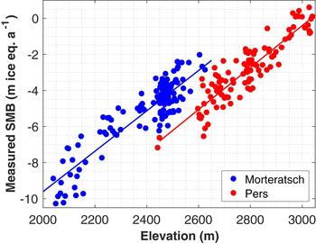
Over the 15-year period, a total of 232 annual mass-balance point measurements are available for the ablation area and around the Equilibrium Line Altitude (ELA) of the Morteratsch glacier complex (Fig. 3). These readings result from annual visits to the glacier, which occur at the very end of September – beginning of October, corresponding to a floating-date system that is very close to the fixed-date system (Cogley and others, Reference Cogley2011). Of the 232 readings, eight have a positive mass balance (up to +0.6 m ice eq a−1) (Fig. 3). A total of 128 readings were performed on Vadret da Morteratsch and 104 on Vadret Pers (see Fig. 1). These readings were obtained from 31 separate stakes (17 on Vadret da Morteratsch, 14 on Vadret Pers), of which 12 stakes have a series of at least 10 years and eight stakes cover the full 15-year period. The entire dataset is available as Supplementary material. For Vadret da Morteratsch, the elevation of the stakes ranges from the front (~2030–2100 m a.s.l. over this period) to ~2600 m a.s.l. (just underneath the icefall, the ‘labyrinth’). Most of this range is covered with stakes, roughly at 100 m height intervals (see also Fig. 1). For Vadret Pers, two SMB observations were taken at the front (~2450 m a.s.l.), but all other measurements are situated between 2600 and 3050 m a.s.l. (~ the ELA). The SMB is significantly lower on Vadret Pers compared with Vadret da Morteratsch (Fig. 3), which is likely related to the orientation and resulting daily insolation cycle for both glaciers. The ablation area of the Pers glacier is oriented towards the WNW (tongue)–NW (upper ablation area) and is more exposed to direct insolation than the Morteratsch glacier, which is exposed to the N and strongly shielded by the high mountain peaks (see also Fig. 1). A simple approach in which a best linear fit (i.e. linear regression) through all stakes is taken clearly illustrates the higher SMB for Morteratsch in the 2000–3000 m elevation range (ablation area):
 $$\eqalign{{\rm SMB}_{\rm MORT} & = 0.01119\; (\pm 0.00098) \;{\rm ELEV} \cr & \quad -31.98 \;(\pm 2.36)\,(R^{2} = 0.80),}$$
 $$\eqalign{{\rm SMB}_{{\rm PERS}} & = 0.01164 \;( \pm 0.00106)\; {\rm ELEV} \cr & \quad -35.31\,( \pm 2.98)\,(R^{2} = 0.82),}$$
where SMBMORT/PERS is the annual measured SMB (in meter ice equivalent), ELEV is the stake elevation (in m a.s.l.) and the uncertainties correspond to the 95% confidence bounds. Based on this very simple approach, for the period 2001–2016, the average ELA for the Morteratsch glacier is expected to occur at 2859 m, which is a slight underestimation compared with remote-sensing observations (Chan and others, Reference Chan, Van Ophem and Huybrechts2009). This is likely related to the fact that the SMB-elevation gradient decreases towards the ELA. For the Pers glacier, the linear correlation suggests that the ELA for this period is at 3035 m, which agrees very well with observations (see Fig. 3). The difference in ELA between both glaciers is typically of the order of 150 m for this period. Direct SMB measurements in the ablation area of the Morteratsch glacier are ~2.1–2.5 m ice eq. a−1 higher than these measured on the Pers glacier at the same elevation. These are large differences in SMB and ELA given the close proximity of both glaciers.

3. DATA HANDLING AND STATISTICAL BACKGROUND
For the MLRA, 120 SMB measurements are considered, which correspond to the eight stakes that cover the whole observational period (i.e. the 15-year record). All eight stakes are in the ablation zone and are in debris-poor areas. Four of these stakes are located on Vadret da Morteratsch and four on Vadret Pers (see Fig. 1). Including SMB measurements from stakes that do not cover this entire period would introduce bias in the anomalies due to the gap in their data record. Since SMB data from the eight stakes covering the full period would be needed to solve these biases, this approach would not add information about total SMB variance.
The SMB stakes undergo elevation changes as time evolves due to their movement along with the glacier flow and due to changes in local ice thickness (Zekollari and others, Reference Zekollari, Fürst and Huybrechts2014; Fischer and others, Reference Fischer, Huss and Hoelzle2015). Over the 15-year period, the elevation change for the eight stakes ranges from −115 m (P33) to −44 m (P21). To account for this effect, all stakes are projected back to their initial elevation (in 2001) based on the SMB-elevation gradients found from the simple linear correlation (Eqns (1) and (2)). For the Pers glacier, this corresponds to 0.0116 m ice eq. a−1 m−1, while for the Morteratsch glacier, this is 0.0112 m ice eq. a−1 m−1. Corrections based on the annual values of the mass-balance gradient lead to almost identical results and do not significantly alter the results as the elevation change is relatively limited and the SMB-elevation gradient varies only little over time.
The individual stake measurements are shown in Figures 4a, b. The highest SMB is observed for the balance years 2003–2004, 2012–2013 and 2013–14, and lowest SMB for 2002–2003 and 2014–2015. The stakes have a consistent annual SMB signal. For these elevation change corrected SMB values, no significant trend is observed over the 15-year period (R 2 = 0.13, p-value F-test = 0.185). The std dev. in SMB per stake over the entire period varies between 0.6 and 0.9 m ice eq. a−1 and is not correlated to elevation (R 2 = 0.04) (Fig. 4c). For the analysis, the elevation-corrected SMB measurements for each stake are converted to perturbations with respect to the 15-year stake mean. As shown on Figure 4d, the annual SMB perturbation is largely similar over the whole ablation area, for both glaciers taken together and for Vadret Pers and Vadret da Morteratsch separately. No link with elevation is observed. This is underscored by the very high correlation (R 2 = 0.85–0.91) between the SMB perturbation of individual stakes and the mean perturbation over all stakes (Table 1). Exceptions are M51 and M62 with a somewhat lower R 2 of between 0.62 and 0.67, where a few individual measurements (M51 in 2005–06 and 2015–16 and M62 in 2008–09 and 2012–13) cause a slight deviation from the mean perturbation. Despite this, the correlation between the perturbation of these individual stakes and the mean perturbation over all stakes is still very significant (p-values of 2 × 10⁻⁴ and 5 × 10⁻⁴, respectively). Furthermore, no link between the meteorological data (temperature and precipitation) and annual SMB elevation gradient is found. The presence of a common SMB signal, which is independent from the location, is a prerequisite for our analyses and is in line with the time-space decomposition as proposed by Lliboutry (Reference Lliboutry1974) and related studies (Meier and Tangborn, Reference Meier and Tangborn1965; Kuhn, Reference Kääb1984; Rasmussen, Reference Rasmussen2004; Eckert and others, Reference Eckert, Baya, Thibert and Vincent2011).
(a) Annual surface mass balance against elevation for different years for the eight selected stakes (before projection to initial elevation); (b) annual surface mass balance against elevation for the eight selected stakes (before projection to initial elevation); (c) standard deviation (σ) per stake over the 15-year period; (d) SMB perturbation for the eight selected stakes for the whole glacier complex and for both glaciers separately. The circles and squares correspond to the individual stakes (cf. panel b).

Correlation (R 2 value and p-value of the F-test) between the eight selected stakes and the mean perturbation (black line on Fig. 4d)

The SMB perturbations over the eight stakes are averaged on an annual basis, and the same is done for the meteorological variables, which are averaged over the two meteorological stations. To assess the glacier's sensitivity to temperature and precipitation changes, which are measured in different units (°C and mm w.e., respectively), these values are standardised through a conversion to a z-score, which corresponds to the number of standard deviations that a value is separated from the mean value.
The correlation between SMB perturbation and meteorological data are tested with MLRA (e.g. Legendre and Legendre, Reference Legendre and Legendre2012):
 $$y = a_{1} x_{1} + a_{2} x_{2} + \ldots + a_n x_n + b.$$
Here y is the dependent variable (also referred to as response variable; the SMB perturbation in this study), a i and b are the regression coefficients and x i are the independent variables (also referred to as predictor variables; the z-score of the meteorological components in this study, i.e. temperature and precipitation). The monthly temperature and precipitation series used in our analyses have a very weak correlation (R 2 = 0.17 when all months are considered, with the highest correlation in spring (MAM): R 2 = 0.21 and lowest correlation in winter (DJF): R 2 = 0.04). They can therefore be considered as being uncorrelated, which is a common approach for MLRAs performed on SMB series (e.g. Lefauconnier and others, Reference Lefauconnier, Hagen, Ørbæk, Melvold and Isaksson1999; Trachsel and Nesje, Reference Trachsel and Nesje2015). Due to the conversion of the meteorological data to a z-score, the regression coefficient (a i) of variables represents the climatic variability of this variable. Under this z-score approach, the standard regression coefficients for temperature and precipitation are directly comparable and, assuming both are entirely uncorrelated, indicate the relative importance of both for the SMB. Furthermore, the standardisation procedure leads to an intercept of the regression analysis (b) that is equal to zero: i.e. under the mean 2001–2016 climatological conditions (z-score of 0 for the independent variables), the mean 2001–2016 SMB is obtained (dependent variable is 0). For each MLRA the error degrees of freedom correspond to the difference between the total number of years (15 in this case) and the number of independent variables in the analysis.
The outcome of each MLRA is expressed as a R 2 value and a p-value for the F-test. The R 2 value corresponds to the fraction of the variability in the response variable that the model explains. The F-test tests for a significant linear regression relationship between the response variable and the predictor variables. The p-value of the F-test, also referred to as calculated probability, is the probability of obtaining a result (a linear correlation) equal to or more extreme than what is observed when the null hypothesis (no linear correlation) is true. The lower the p-value, the higher the confidence (lower significance level) at which the null hypothesis (no linear correlation) can be rejected.
In our MLRA, we opt for the mean monthly temperature and not for the monthly average of the daily maxima, as air temperature can also cause melt during the night time (cf. Letréguilly, Reference Letréguilly1988). The difference between results obtained with mean monthly temperature and the monthly average of the daily maxima is however very limited as the trends in both are very similar (R 2 = 0.97).
4. METEOROLOGICAL DATA MLRA
4.1. Variable selection
Initially, meteorological variables that best describe the observed SMB are considered as time clusters, i.e. as continuous time periods (4.2.), which is in line with most previous studies. Subsequently, a new method is introduced, where all possible monthly combinations (full-spectrum analysis) are considered for describing the observed SMB signal (4.3.). For all MLRAs, the goal is to describe most of the observed SMB variance, by using as few predictor variables as possible. Adding additional predictor variables increases the fraction of the SMB variation that can be explained, but reduces the degrees of freedom. To assess whether it is justified adding additional predictors (i.e. to avoid overfitting), the p-value of the F-test is considered, which should be as low as possible.
4.2. Continuous time periods
Annual periods are used at first (4.2.1.), after which a subdivision is made into half-years (4.2.2.), seasons (4.2.3.) and finally months (4.2.4.).
4.2.1. Annual time period
As a first test, the mean annual temperature (T ann) and the total annual precipitation (P ann) are used to explain the observed SMB variation (i.e. MLRA with 13 error degrees of freedom). An MLRA between these two variables and the measured SMB reveals that ~22% of variance in SMB can be explained by these annual anomalies (R 2 = 0.22, see Fig. 5a and Table 2). The weak significance of this model in describing the measured SMB variance is reflected in the high p-value for the F-test (0.229). Despite the weak correlation, the signs of the variables are logical, being negative for T ann (−0.35, negative correlation between temperature and SMB) and positive for P ann (+0.20, positive correlation between precipitation and SMB).
Observed SMB perturbation and modelled SMB perturbation based on multiple linear regression analysis (MLRA) using the following two predictors: (a) annual temperature (T ann) and annual precipitation (P ann), (b) summer half-year temperature (T SHY) and winter half-year precipitation (P WHY), (c) average May, June, July temperature (T MJJ) and winter half-year precipitation (P WHY). The black line is the observed SMB (cf. black line in Fig. 4d), the grey line is the calculated SMB signal resulting from the MLRA.

Multiple linear regression analysis (MLRA) between z-score standardised meteorological variables (averaged over Segl-Maria and Samedan) and observed SMB perturbations for eight selected stakes covering the period 2001–2016

4.2.2. Half-year time period
In the second step, the year is subdivided in a winter half-year (WHY), consisting of fall (OND: October–November–December) and winter (JFM: January–February–March), and a summer half-year (SHY), which consists of spring (AMJ: April–May–June) and summer (JAS: July–August–September). These monthly clusters rather agree with the glaciological seasons than with the meteorological seasons. They are chosen so that the fall season (OND) starts just after the field measurements, broadly corresponding to the beginning of the accumulation season (i.e. the beginning of the water/hydrological year).
From the MLRA, the importance of the SHY temperature (T SHY) is clear, as this predictor variable alone already explains 35% of the observed SMB variance (R 2 = 0.35). Without this variable, almost none of the SMB variance can be explained in a MLRA with two predictor variables (<4%; p-values F-test above 0.8) (Table 2). The SHY temperature and the WHY precipitation account for almost half of the observed SMB variance (46.4%, Fig. 5b), which rejects the null hypothesis (no linear correlation) at the 5% level (p-value F-test 0.024), but which still leaves a very large part of the SMB unexplained. The larger absolute regression coefficient T SHY (−0.51) compared with P WHY (0.25) indicates a relatively higher importance of the SHY temperature. This is also supported by the fact that the SHY temperature combined with the (supposedly) not very relevant SHY precipitation can explain almost a similar fraction of the observed SMB variance (R 2 = 0.39, see Table 2).
4.2.3. Seasonal time period
In this analysis, the predictor variables were split up in seasonal components, i.e. spring (AMJ), summer (JAS), autumn (OND) and winter (JFM). Combined with the possibility of still using the variables at the half-year time period (WHY and SHY, see previous section), this allows for 36 (62) possible combinations for MLRAs with one temperature and one precipitation predictor variable. With two predictor variables, most of the SMB variability is described by the SHY temperature and the WHY precipitation (cf. Section 4.2.2.), followed by combining the spring temperature and the WHY precipitation (R 2 = 0.46, p-value of F-test = 0.0251). With three predictor variables, most of the variation can be described through the spring and summer temperature normalised anomalies as two separate variables and the WHY normalised precipitation anomaly as one variable: SMB = −0.49 T spr − 0.21 T sum + 0.23 P WHY. The R 2-value of 0.55 is higher than the one for the model based on TSHY and PWHY (see Section 4.2.2.), but the p-value of the F-test (0.0286) is also higher (suggesting overfitting) as the error degrees of freedom are in this case reduced to 12 (vs 13 in the previous analysis). Although the correlation remains relatively low, which suggests that a more refined choice of time periods is needed, the regression coefficients indicate a larger importance for spring temperature compared with the summer temperature.
4.2.4. Monthly time period
A more in-depth analysis, where all different combinations of clustered (subsequent) months are allowed, suggests that the SMB variance is best described by the average May–June–July temperature (T MJJ) and the total precipitation from October to March (i.e. the WHY precipitation, Table 2). This MLRA is statistically very significant (p-value F-test of 1.02 × 10⁻⁵) and accounts for 85.3% of the variance in measured SMB (Fig. 5c), with a clear dominance of the MJJ temperature (regression coefficient of −0.65) compared with the WHY precipitation (regression coefficient of 0.24).
4.3. Discontinuous time periods (full-spectrum analysis)
MLRAs are now performed between the SMB series and all possible monthly combinations of temperature and precipitation. This new setup is still based on two predictor variables, i.e. one for temperature and one for precipitation, and the error degrees of freedom are therefore still equal to 13. For each MLRA, a different combination of temperature and precipitation months is selected and analysed, resulting in a total of 16.8 million (=224) combinations. The total number of combinations arises from combining all the 24 different variables, 12 for the temperature months and 12 for the precipitation months, in every possible way. Performing such a large number of MLRAs is now possible because of increased computational power, which was a limiting factor in the past (e.g. Letréguilly, Reference Letréguilly1988). For each MLRA, the temperature predictor variable is the mean temperature of the selected temperature months, while the precipitation variable is the precipitation sum of all selected precipitation months. As was the case for the continuous time period MLRAs (Section 4.2.), both predictor variables are expressed as anomalies through a z-score conversion to allow for a direct comparison of their individual contribution to explain the SMB series.
The R 2 values of the 224 MLRAs have a right-skewed distribution (skewness of +0.759), with a peak at R 2 = 0.1–0.12 (see Fig. 6a). R 2 values range between 0 and 0.9086. The highest R 2 value (0.9086) is obtained from the mean May–June–July–October–November temperature and the February–May–June–December precipitation. This obtained unique combination is however very sensitive to even small changes in observed SMB, and it is therefore more relevant to consider an ensemble of combinations. The 50 combinations that best describe the observed SMB variance (Fig. 6b; Fig. 7), i.e. the ones with the highest R 2 values (R 2>0.86088), have a clear monthly pattern. For all 50 combinations, the June and July temperatures are included (100% probability inclusion (p.i.)), while 49 combinations include the May temperature (98% p.i.) (Fig. 6c). Subsequently, the October temperature (40% p.i.) and November temperature (24% p.i.) sometimes appear in the top 50 combinations, but for all other months, the effect of the temperature on the SMB variations is close to negligible. For precipitation all months are well represented in the top 50 combinations, except for July and August (Fig. 6d). The most crucial months seem to be those before and at the onset of the ablation season (February–March–April–May–June) and those at the beginning of the accumulation season – early winter (October–November–December).
(a) Probability density of R 2 values for MLRA for all (16.8 million) possible combinations of months. The green area corresponds to R 2 range between 0.74 (lower limit 0.1% highest R 2 values) and 0.86 (lower limit 50 highest R 2 combinations), the red area is the range of the 50 combinations with the highest R 2 value. (b) Zoom on the 50 MLRAs with highest R 2 values, which are visually non-detectable in (a). (c) and (d) Probability that a particular month's temperature or precipitation is included in the 50 combinations with highest R 2 value. (e) and (f) Probability that a particular month's temperature or precipitation is included in the top 0.1% combinations (16 777 combinations) with the highest R 2 value.


When considering the top 0.1% of all combinations, which corresponds to the 16 777 combinations with an R 2 value higher than 0.73599, the importance of the monthly temperatures remains almost unaltered (Fig. 6e). July is the most common month in this selection (98.8% p.i.), closely followed by May (93.3% p.i.), June (92.4% p.i.), and subsequently by October (57.9% p.i.) and November (37.2% p.i.). For the precipitation, the importance of the individual months changes slightly when considering this larger ensemble of combinations (Fig. 6f) compared with the top 50 combinations (Fig. 6d). The summer months still have a slightly more limited contribution to the observed SMB, but for the other months, no clear pattern is obtained and all months have a fairly similar occurrence in the 0.1% top combinations (varying between 41.2 and 73.5% p.i.).
5. DISCUSSION
5.1. Robustness correlations and time-series length
The MLRAs performed for different time periods (annual, half-year, seasonal and monthly) are mutually consistent, which indicates that the correlations are robust. The full-spectrum method, in which discontinuous periods are also considered, supports this, and the dominant months from the continuous time period analysis (May, June, July temperature and WHY precipitation) are confirmed. Furthermore, the importance of other months’ temperature (October, and to a lesser extent November) and precipitation (spring: April, May, June) also appears.
The robustness and significance of the results is supported by statistical evidence. For the best models, low p-values for the F-test and high R 2-values are obtained (R 2 > 0.86 for the best 50 combinations of the full-spectrum analysis). In contrast, when performing the full-spectrum analysis with series of random SMB data and/or meteorological data, the 50 best combinations of monthly meteorological variables are typically only able to explain between 50 and 70% of the SMB variance, significantly less than the 86% found here from the real data.
The length of the record, 15 years, is thus sufficient to obtain meaningful regression coefficients. The main finding of a very limited effect of August and September temperature in fact already appears when a period of 10 years (e.g. 2001–2011) is considered (not shown here). The sufficient length of the 15-year record agrees with the findings by Letréguilly and Reynaud (Reference Letréguilly and Reynaud1989) who state that at least 10 years are needed to obtain qualitative regression coefficients, and Vincent and Vallon (Reference Vincent1997) who mention a 5–10-year period as a minimum.
5.2. Temperature dominance
The results from the MLRAs indicate that there is a strong correlation between temperature and observed SMB, which is the cornerstone for various widely used simplified SMB models (e.g. Reeh, Reference Reeh1989; Hock, Reference Hock2003; Braithwaite and others, Reference Böhm2013). This strong SMB dependence on temperature is also in line with the findings from a previous simple surface energy balance (SEB) modelling study on the Morteratsch glacier (Nemec and others, Reference Nemec, Huybrechts, Rybak and Oerlemans2009). Nemec and others (Reference Nemec, Huybrechts, Rybak and Oerlemans2009) parameterised the longwave radiation and the turbulent heat fluxes as a function of temperature (cf. Oerlemans, Reference Oerlemans2001) and were able to closely reproduce the observed SMB.
The SEB in the ablation area of the Morteratsch glacier complex is mainly driven by the radiation components and the sensible heat flux, while the latent heat flux is much smaller (Klok and Oerlemans, Reference Klok and Oerlemans2002, Reference Kuhn2004). Notice that this is strongly related to the climatic conditions and the location of the glacier (mid-latitude maritime glacier), and in other settings (e.g. continental, polar, tropical), the importance of the individual SMB components may strongly vary (e.g. Benn and Evans, Reference Benn and Evans2010). The fact that temperature explains a very large fraction of the observed SMB variations partly results from its direct influence on the sensible heat flux, which is one of the dominant fluxes in the glacier SEB. Furthermore, temperature correlates with the short-wave radiation component, as a higher temperature leads to surface melt and lowers the surface albedo, which in turn increases the net shortwave radiation. The longwave radiation, despite being the first source of the energy balance (Klok and Oerlemans, Reference Klok and Oerlemans2002), has a limited interannual variability and is therefore of limited importance when considering SMB variations over time (cf. Sicart and others, Reference Sicart, Hock and Six2008).
MLRAs in which additionally radiation components are considered (e.g. Lefauconnier and others, Reference Lefauconnier, Hagen, Ørbæk, Melvold and Isaksson1999) hardly improve the fraction of the observed SMB that can be explained. For instance, if the total monthly hours of sun are added to the analysis, the fraction of the SMB variance that can be explained is almost unaltered. The monthly hours of sun are not significant at the 5% significance level given the other terms (temperature and precipitation for selected months) in the MLRA. Notice that the same is true when a second temperature variable is introduced (i.e. working with three predictor variables), adding additional complexity to the MLRA, with limited to no added value (case of overfitting, as the p-value of the F-test increases).
5.3. Limited effect of mid- to late-summer conditions on SMB variability
In the ablation area of alpine glaciers, most of the surface mass loss occurs during summer, which at the monthly time period used in this study corresponds to July, August and September. During this period, the snow cover that protects the glacier through its high albedo is removed and the glacier ice (low albedo) is directly exposed. Due to its lower albedo, an ice-covered surface absorbs more of the incoming radiation compared with a snow-covered surface and therefore experiences more melt.
According to the MLRA conducted here, the meteorological conditions in August and September have a very limited effect on the interannual SMB variability, as models without these components are able to explain more than 90% of the observed changes in SMB (Fig. 6). The precipitation during these 2 months typically occurs as rain and also the temperature of these months was found to have a very limited contribution to the observed SMB variability. On the other hand, the WHY precipitation and the meteorological conditions at the start and at the end of the ablation season have a much larger effect on the interannual SMB variability in the ablation area of the Morteratsch glacier complex. The latter corresponds to the mid- to late-spring precipitation (April, May), the late-spring to early-summer temperature (May, June, July) and early-autumn precipitation and temperature (October). The WHY precipitation determines the winter balance and determines the thickness of the snow pack at the beginning of the ablation season. The May–June–July temperatures subsequently determine the snow ablation intensity and the precipitation type (snow/rain). A lower mean monthly temperature increases the chance of a precipitation event being a snowfall event, which increases the SMB. The importance of autumn (October and to a lesser extent November) conditions is not surprising, as this period largely determines the transition from the ice-covered to the snow-covered ablation area. Often ice melt still occurs after the SMB measurements (late September to early October), as field observations determined that the ablation area is often not entirely snow-covered at this time.
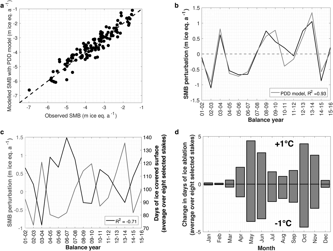
The results from the MLRAs thus suggest that the length of the ablation season, rather than its intensity, determine the interannual SMB variability here. This is related to the interannual melt differences between the summer seasons, which are believed to be much smaller than the intra-annual contrast between snow and ice melt (contrast between the seasons) (cf. Durand and others, Reference Durand2009; Thibert and others, Reference Thibert, Eckert and Vincent2013). Results from a straightforward positive-degree-day (PDD) calculation support the dominant effect of the ice ablation season duration on the glacier's ablation area SMB. The PDD model is run at an hourly time step, and the 2 m temperature at each stake is derived from an interpolation between measured temperatures at Samedan (1708 m) and Corvatsch (3302 m). Precipitation is upscaled from Samedan with an elevation gradient of 1.0 mm w.e. m−1, based on field measurements in the glacier's accumulation area (Sodemann and others, Reference Sodemann, Palmer, Schwierz, Schwikowski and Wernli2006; Nemec and others, Reference Nemec, Huybrechts, Rybak and Oerlemans2009). A distinction is made between snowfall and rainfall depending on the air temperature. The degree-day factors (DDF) for snow and ice are calibrated in order to minimise the RMSE between observed and modelled SMB. For the eight stakes over the 15-year period, an RMSE of 0.385 m w.e. a−1 is obtained (Fig. 8a) with a DDF for snow/ice of 2.8/5.4 mm ice eq. per degree day for the Morteratsch glacier, and 3.5/6.6 mm ice eq. per degree day for the Pers glacier. These DDFs are in good agreement with the values found for other glaciers in the European Alps (e.g. Hock and others, Reference Hock, Iken and Wangler1999). Despite the PDD model's simplicity (e.g. shading effects from the surrounding mountains and refreezing/retention of meltwater in the snowpack are not accounted for), the observed SMB (Fig. 8a) and its interannual variability (R 2 = 0.93, Fig. 8b) are closely reproduced. The PDD model indicates that the number of ice ablation days (averaged over the eight stakes) is strongly anticorrelated with the SMB perturbation (Fig. 8c). The variation in ice ablation days is ~70% anticorrelated to the modelled SMB variance (R 2 = −0.71) and 60% anticorrelated to the observed SMB (R 2 = −0.60). The PDD simulations furthermore indicate that the temperature in the early- and late-ablation season has the largest influence on the ice ablation season length (Fig. 8d, shown for a temperature bias of −1 and +1°C). The effect of changes in the July temperature on the ice ablation season length is found to be limited, as this is usually the warmest month of the year.
(a) Observed vs modelled annual SMB through a PDD approach for the eight selected stakes over the 15-year period. (b) Observed SMB perturbation (black line, cf. Fig. 5) and PDD modelled (grey line) SMB perturbation. (c) PDD modelled SMB perturbation (grey line) and days of ice ablation (averaged over eight selected stakes, black line). (d) Change in number of ice ablation days for a monthly temperature increase/decrease of 1°C, as obtained from the PDD model.
The importance of the WHY precipitation and early- and late-ablation season meteorological conditions is also clear when analysing the 2 years with the lowest SMB (2002–03 and 2014–15) and the 3 years with the highest SMB (2003–04, 2012–13 and 2013–14) (Table 3). The lowest SMB (2002–03) over the period can be explained by the 2003 European heat wave (Beniston, Reference Beniston2004; García-Herrera and others, Reference García-Herrera, Díaz, Trigo, Luterbacher and Fischer2010) (z-score of 1.41 for 2003 T sum), but also the high temperatures in October 2002 and May 2003 have had an important role (z-score of 1.58 for T OctMayJunJul). Notice that the 2002–03 SMB year also had a high winter precipitation (524.4 mm vs an average of 308.8 mm, z-score of 1.89), but this is almost entirely due to the extremely high November precipitation, which is the highest monthly precipitation for the entire period considered in this study 16-year period (392.2 mm, see Fig. 2). A substantial fraction of the precipitation occurred on November 14–16 when temperatures in the ablation area of the glacier were varying between −3.5 and +3.5°C (Fig. 9). It is therefore likely that (a part of) the precipitation over this time period did not occur as snow, which illustrates the aforementioned role of autumn temperatures in delimiting the rain/snowfall regime. The snow accumulation that may have occurred in November likely melted during late autumn and early winter, which winter had moreover a very dry period later on (P Dec→Mar for this balance year is the lowest of the record, 58.8 vs 136.3 mm on average; z-score of −1.26). The year with the second most negative SMB (2014–15) had similar average temperatures for the months of May–June–July–October as 2002–2003, but probably the SMB was slightly less negative due to the higher December–March precipitation, which was close to average (133.6 mm, z-score of −0.05).
Hourly precipitation at Samedan meteorological station and hourly temperature at Samedan meteorological station (1708 m) and Corvatsch meteorological station (3302 m). Temperature series at 2200 m (lowest elevation of SMB measurements) and 2900 m (highest elevation of SMB measurements) are derived through linear interpolation between the Samedan and Corvatsch series. The shaded area roughly corresponds to the rain/snow threshold.

Meteorological variables averaged over the stations of Samedan and Segl-Maria for the 2001–2016 period for selected years. Values between brackets indicate the respective z-score of the values

The 3 years with the highest SMB (2003–04, 2012–13 and 2013–14) are all characterised by low average May–June–July–October temperatures. The limited importance of August and September temperatures on the SMB variability is also illustrated by the relatively high SMB for the years 2003–04 and 2012–13, which years respectively had an average (z-score of −0.05) summer (July–August–September) and an above-average warm summer (11.05 vs 10.69°C on average, z-score of 0.50). The most positive SMB year, 2013–14, had relatively low May–June–July–October temperatures, and here the very high P WHY (z-score of 1.39)/P Dec−Mar (z-score of 2.48) played a major role.
5.4. Comparison to other studies
Most studies correlating temperature and precipitation data to SMB variations found summer temperatures to be the key component. Martin (Reference Martin1978) explained 77% (R 2 = 0.77) of the 1949–75 SMB variance of Glacier de Sarennes by means of maximum summer temperature, precipitation from October to May and a June precipitation component (three predictor variables). For glaciers in the Swiss Alps, Chen and Funk (Reference Chen and Funk1990) used the mean summer temperature and the mean annual precipitation to describe the SMB variations and with this they could explain between 49 and 81% of the observed variance. For these studies on Alpine glaciers, the temperature variations dominate the SMB compared with the precipitation variations, which is also the case in our analysis and confirmed in other SMB modelling studies (e.g. Oerlemans and Reichert, Reference Oerlemans and Reichert2000). In a study on Austre Brøggerbreen (Svalbard) (Lefauconnier and Hagen, Reference Lefauconnier and Hagen1990), 77% of the 19-year net SMB series is explained by the July and August PDDs, which are a measure for air temperature, combined with precipitation from October to May. Later this was updated to 66% of the SMB variance being explained for a 28-year time series by Lefauconnier and others (Reference Lefauconnier, Hagen, Ørbæk, Melvold and Isaksson1999). In a recent study, Trachsel and Nesje (Reference Trachsel and Nesje2015) analysed the SMB of eight Scandinavian glaciers using statistical models and found that summer temperature and winter precipitation explained more than 70% of the variance for maritime glaciers, and between 50 and 70% for continental glaciers.
It is noteworthy that the early- and late-ablation season conditions (e.g. temperatures and precipitation in April, May, June and October), which are key in explaining the SMB variations for the Morteratsch glacier complex, are never included in the above analyses. An exception is the study by Letréguilly (Reference Letréguilly1988) where the June and July temperatures (without August and September) are combined with the October–March precipitation to explain ~70% of the SMB variations for Peyto glacier (Rocky Mountains, Canada). In the same study, the late-spring conditions (T May,June,Jul,Aug and P Oct→May) are also incorporated to explain 65–75% of the SMB variations for Sentinel glacier and Place glacier (Coast Mountains, Canada).
Important to note as well is that the above-mentioned studies consider the glacier-wide SMB, while our analysis is based on stakes only from the glacier's ablation area. In the accumulation area, the snow-ice cover contrast is not present, but also here a seasonal albedo contrast exists. The winter and spring fresh snow have a high albedo, but as the summer advances the snow cover metamorphoses and becomes dirtier (Oerlemans and others, Reference Oerlemans, Giesen and van Den Broeke2009), which in combination with melt and rainfall events (Oerlemans and Klok, Reference Oerlemans and Klok2004) leads to an albedo decrease. Therefore, the differences between the ablation area SMB signal and the glacier-wide SMB signal are expected to be limited. The difference between our results, with a limited effect of August and September conditions and other studies is therefore also believed to be partly linked to differences in methodology (e.g. point measurements vs glacier-wide SMB, see further) and the full spectrum of monthly combinations considered here.
Also for the continuous month approach (4.2.4), i.e. the classic approach, the correlations obtained are very high for our 15-year record (Fig. 5c) compared with other studies. This may again be linked to opting for a different variable than the widely used June–July–August temperatures (here May–June–July is used), but may in part also be related to the quality and homogeneity of the data used in this study. First of all, the data from the MeteoSwiss stations is from a recent period and highly reliable, which is not always the case in earlier studies, as argued for instance by Letréguilly (Reference Letréguilly1988). Especially older temperature and precipitation measurements contain biases and need to be corrected to homogenise the time series (e.g. Böhm and others, Reference Braithwaite, Raper and Candela2010). Second, the systematic error on the Morteratsch SMB is believed to be relatively limited and similar in magnitude over time, as all measurements occurred by the same group of scientists, using the same methodology and with the same materials. This is often not the case and for extended periods of time, the measurement errors can be very large, up to 20–40 cm and even more for older stakes (Letréguilly and Reynaud, Reference Letréguilly and Reynaud1989). Finally, we opted to correlate the meteorological data directly to our SMB measurements, instead of using a spatially averaged/glacier-wide SMB (cf. Vincent and others, Reference Vincent and Vallon2017). The eight stakes used in this study cover the whole period and move only very little, which is corrected with high-precision GPS measurements. Other studies consider spatially averaged SMB or (partially) modelled SMB, which adds an additional uncertainty.
6. CONCLUSION AND OUTLOOK
In this study, we analysed a dataset consisting of 15 years of SMB measurements in the ablation area and around the ELA of the Morteratsch glacier complex, and attempted to describe the SMB variability through a minimal statistical approach. The observed interannual SMB variance is very similar for both glaciers and can largely be explained (>90%) by combining monthly temperature and precipitation data from nearby meteorological stations. The fact that almost the entirety of the SMB variance can be explained by a simple MLRA with one temperature and one precipitation variable makes it redundant to add additional predictor variables (e.g. radiation, additional temperature or precipitation variable) to the analysis. The full-spectrum method introduced in this study relies on increased computational power, which was a limiting factor in the past, and considers the contribution of every month's temperature and precipitation, which are combined in these two predictor variables. The MLRA indicates that the spring-/early-summer and autumn meteorological conditions play a crucial role, as they determine the length of the ablation season. High temperatures and low precipitation in spring advance the transition from a snow- to an ice-covered surface, while in autumn they favour a prolonged ice ablation season. Furthermore, temperatures during these months also influence the SMB perturbation by affecting the precipitation type (rain/snow) over the ablation area of the glacier. The mid- to late-summer (August and September) conditions are found to have only a minor effect on the annual SMB perturbation. These findings are supported by output from a simple PDD model, indicating that early- and late-melting season meteorological conditions are the main drivers for the ice ablation season duration, which is itself strongly anticorrelated to the SMB perturbation. The widely used June–July–August (JJA) temperature index may therefore not always be the most appropriate variable to describe SMB variability through statistical correlation.
Applications of the full-spectrum method to other glaciers and other SMB series will be useful to better understand the meteorological station representativeness, the impact of their distance to the measurements and contrasts between ablation/accumulation measurements and seasonal/annual SMB measurements. Through its minimal character, relying on as few predictor variables as possible, the method is an interesting alternative/complementary approach to the more classic, well-established stepwise selection procedures (e.g. Tinsley and Brown, Reference Tinsley and Brown2000; Whittingham and others, Reference Whittingham, Stephens, Richard and Freckleton2006). In future works, the threshold delimiting the ‘best’ combinations (here set at the best 50 combinations and the top 0.1% combinations) will have to be investigated and could potentially be changed for other studies. In this study, the temperature dependence is very clear, but this is less the case for precipitation. For the latter, the monthly signal changes as the threshold changes, which is related to the fact that the precipitation contributes less to the observed SMB variance than the temperature. Possible extension of the method presented here could for instance separate between the SMB in the ablation and accumulation area, or between winter and summer SMB, if the necessary measurements are available.
SUPPLEMENTARY MATERIAL
The supplementary material for this article can be found at https://doi.org/10.1017/jog.2018.18
ACKNOWLEDGEMENTS
We are grateful to everyone who helped to collect the SMB data on the Morteratsch glacier complex over the past 15 years and thank MeteoSwiss for making all meteorological data available. Harry Zekollari performed this work through a PhD fellowship of the Research Foundation – Flanders (FWO-Vlaanderen) and finalised this research during a research stay at ETH Zürich, financed by a travel grant for a long stay abroad from the Research Foundation Flanders (grant No. V427216N). Matthias Huss is thanked for the fruitful discussions. We thank the Associate Chief Editor H. Jiskoot, the Scientific Editor N. Eckert, and three anonymous reviewers whose comments and suggestions greatly helped to improve the manuscript.


 Open access