


Social media summary
Wealthy urban areas most responsible for Europe's global biodiversity footprint.
1. Introduction
The International Union for Conservation of Nature and Natural Resources (IUCN) estimates that more than 28,000 species are presently threatened with extinction (IUCN 2019). The primary causes of biodiversity loss include habitat loss, climate change, pollution, overexploitation and invasive species (Millennium Ecosystem Assessment 2005; WWF 2016). While the production of goods like coffee or beef is a direct domestic driver for such environmental pressures, the demand for these goods often lies in other regions of the world (Lenzen et al. Reference Lenzen, Moran, Kanemoto, Foran, Lobefaro and Geschke2012; Chaudhary & Kastner Reference Chaudhary and Kastner2016; Moran & Kanemoto Reference Moran and Kanemoto2017; Verones et al. Reference Verones, Moran, Stadler, Kanemoto and Wood2017; Wilting et al. Reference Wilting, Schipper, Bakkenes, Meijer and Huijbregts2017; Wiedmann & Lenzen Reference Wiedmann and Lenzen2018). European countries in particular are responsible for a large share of environmental pressures originating abroad (Tukker et al. Reference Tukker, Bulavskaya, Giljum, Koning, Lutter, Simas and Wood2016; Wood et al. Reference Wood, Stadler, Simas, Bulavskaya, Giljum, Lutter and Tukker2018).
Household consumption is an endpoint of global supply chains and can thus be considered to be a major driver of environmental burdens (Ivanova et al. Reference Ivanova, Stadler, Steen-Olsen, Wood, Vita, Tukker and Hertwich2016). What shapes household consumption will therefore have an impact on global biodiversity loss. Additionally, the composition of household demand is neither static, nor equal across different groups, but rather depends on multiple socio-cultural and economic factors (Froemelt et al. Reference Froemelt, Dürrenmatt and Hellweg2018). As countries and the world as a whole become increasingly urban, it is important to understand how this urbanization process could lead to overall changes in the aforementioned composition of household demand. Do urban, semi-urban and rural households have similar consumption preferences? How much does urbanization alone, rather than changes in income or household size, influence changes in consumption preferences? Whilst the role of urbanization in influencing household carbon footprints has been well studied (Jones & Kammen Reference Jones and Kammen2014; Kanemoto et al. Reference Kanemoto, Moran, Lenzen and Geschke2014; Wiedmann et al. Reference Wiedmann, Chen and Barrett2016; Moran et al. Reference Moran, Kanemoto, Jiborn, Wood, Többen and Seto2018), there is no assessment for biodiversity footprints, which are associated with different consumption categories. That is, biodiversity footprints are associated majorly with food and fibre, whereas carbon footprints are more associated with metals, complex products and services. And while urbanites in wealthy countries tend to have lower emissions, urbanization in developing countries is often linked to increases in wealth and thus higher footprints compared with rural households. Hence, findings on the relationship between urbanization and emissions might differ from those between urbanization and biodiversity footprints.
This paper proceeds as follows: we first discuss the study methodology, after which we present European biodiversity footprints on regional, national and sub-national levels, with a focus on urban vs rural consumption patterns. We outline the influence of selected socio-economic drivers, give detailed accounts of species losses embodied in trade, and describe the role of different product sectors and impact categories. Finally, we discuss these results with regard to current socio-economic developments, and future research.
2. Materials and methods
Much traditional environmental impact analysis studies impacts associated with production. The footprint concept reallocates, through trade and transformation steps, those impacts of primary producers to the households whose final demand ultimately induces them. Thus, for instance, a consumer buying palm oil, or products containing palm oil, may be considered responsible for forest losses in Indonesia and other environmental burdens that occurred along the supply chain of the palm oil product.
To implement this in the present study, we establish a standard environmentally extended Leontief demand-pull model (Leontief Reference Leontief1936, Reference Leontief1970; see also SI6) using a global multi-regional input-output (MRIO) table to estimate consumption footprints. The MRIO database includes detail on average household consumption patterns in each country, but for this study we disaggregated that by incorporating data from consumer expenditure surveys (CESs) in order to obtain detail on consumption patterns by various socio-economic variables. Additionally, the MRIO database natively describes only the physical resources required to satisfy consumption, e.g. hectares of wheat cultivated, cubic metres of roundwood, etc. To evaluate not just the resource demands of consumption but estimate the full ecosystem impact of that consumption, we extend the MRIO model with a life cycle impact assessment (LCIA) model (Verones et al. Reference Verones, Moran, Stadler, Kanemoto and Wood2017). LCIA is commonly used within life cycle assessments (LCA) as a modelling step to convert physical resource demands into estimates of how impactful those pressures are on ecosystems. Extending pressure footprints from MRIO with an LCIA model allows us to model the potential consequences on biodiversity and thus helps to highlight the potential impacts. The analyses were conducted for the years 2005 and 2010.
2.1. Environmentally extended MRIO analysis
Various methods exist for analysing environmental impacts. Although bottom-up approaches such as LCA allow for comparatively higher detail, namely analyses on product or technology level, the top-down accounting method MRIO is preferable for national or regional assessments because of the complete coverage of supply chains and the avoidance of truncation errors (Majeau-Bettez et al. Reference Majeau-Bettez, Strømman and Hertwich2011; Wiedmann & Barrett Reference Wiedmann and Barrett2013; Steen-Olsen et al. Reference Steen-Olsen, Wood and Hertwich2016). MRIO analysis covers both inter-industry and final demand in multiple regions and their bilateral trade interlinkages. By including environmental extensions, MRIO can track environmental pressures associated with trade flows of goods and services.
Environmentally extended MRIO (EE-MRIO) is an established and well-described approach for analysing footprints and environmental burdens associated with supply chains and consumption (Leontief Reference Leontief1936, Reference Leontief1970; Miller & Blair Reference Miller and Blair2009; Kitzes Reference Kitzes2013; Wiedmann & Lenzen Reference Wiedmann and Lenzen2018; see also SI6 for a description of a basic input-output model). EE-MRIO reattributes emissions and resource uses within a nation (production-based account) through multiple trade and transformation steps to final consumers (consumption-based account; Wiebe & Yamano Reference Wiebe and Yamano2016; see SI1 for an introduction into both variations). EE-MRIO analysis has been used in numerous previous studies for calculating footprints regarding environmental pressures (see SI2 for a detailed overview of MRIO applications), e.g. greenhouse gas emissions (Kanemoto et al. Reference Kanemoto, Moran and Hertwich2016; Wiedmann et al., Reference Wiedmann, Chen and Barrett2016; Moran et al., Reference Moran, Kanemoto, Jiborn, Wood, Többen and Seto2018), land use (Ewing et al., Reference Ewing, Hawkins, Wiedmann, Galli, Ertug Ercin, Weinzettel and Steen-Olsen2012), material requirements (Wiedmann et al. Reference Wiedmann, Schandl, Lenzen, Moran, Suh, West and Kanemoto2015; Giljum et al. Reference Giljum, Wieland, Lutter, Bruckner, Wood, Tukker and Stadler2016; Tukker et al. Reference Tukker, Bulavskaya, Giljum, Koning, Lutter, Simas and Wood2016), water stress (Lenzen et al. Reference Lenzen, Moran, Bhaduri, Kanemoto, Bekchanov, Geschke and Foran2013; Lutter et al. Reference Lutter, Pfister, Giljum, Wieland and Mutel2016; Mekonnen & Hoekstra Reference Mekonnen and Hoekstra2011), or threatened biodiversity (Lenzen et al. Reference Lenzen, Moran, Kanemoto, Foran, Lobefaro and Geschke2012; Moran & Kanemoto Reference Moran and Kanemoto2017).
For our analytical EE-MRIO model, we used data from the EXIOBASE MRIO database (Tukker et al., Reference Tukker, Koning, Wood, Hawkins, Lutter, Acosta-Fernández and Kuenen2013; Wood et al., Reference Wood, Stadler, Bulavskaya, Lutter, Giljum, Koning and Tukker2015; Stadler et al., Reference Stadler, Wood, Bulavskaya, Södersten, Simas, Schmidt and Tukker2018) to calculate consumption-based accounts. EXIOBASE v3.4 represents the world economy for the period 1995–2011, distinguishing between 28 EU member countries, 16 major economies, and five rest of the world (RoW) regions, each of the above with a sectoral detail of 163 industries by 200 products. Moreover, EXIOBASE includes an extensive account of environmental pressures, covering a variety of emissions and resource uses (see section 2.4). The rationale for choosing EXIOBASE (over other MRIO databases such as Eora, WIOD or GTAP; see SI3 for a comparative overview) was twofold: first, it provides the highest sector resolution in comparison with other MRIO databases, and second, its individual representation of European countries allowed for a satisfying CES-MRIO data fit.
2.2. Consumer expenditure survey data reconciliation
While the applied EE-MRIO model in its original form provides information on household final demand per country, no further disaggregation of it with respect to socio-economic variables is provided. CESs contain this information, so that complementing the EE-MRIO model with CES data allows the analysis of household final demand on a virtual sub-national level for a multi-region (Steen-Olsen et al. Reference Steen-Olsen, Wood and Hertwich2016; Ivanova et al. Reference Ivanova, Vita, Steen-Olsen, Stadler, Melo, Wood and Hertwich2017).
Eurostat's CES data (Eurostat 2018b) stems from annual large-scale household budget surveys conducted by National Statistical Institutes (Eurostat 2018a). These have been run every 5–6 years since 1988 with 2010 being the newest comprehensive dataset available (Eurostat 2015). 2005 data also had good country coverage.
The extension of the present EE-MRIO model with CES data required several reconciliation steps, the procedure of which followed to a large extent the approach taken by Steen-Olsen et al. (Reference Steen-Olsen, Wood and Hertwich2016) and Ivanova et al. (Reference Ivanova, Vita, Steen-Olsen, Stadler, Melo, Wood and Hertwich2017), and is described in detail in SI4. Essential stages were the upscaling of country-specific mean consumption expenditure per household to the national level, structured by socio-economic parameters and sectors according to the COICOP classification (COICOP is the acronym of ‘Classification of Individual Consumption according to Purpose’; United Nations Statistics Division 2018); the accounting for underreporting, i.e. including detail on the difference between household expenditures reported in CES and MRIO data (Bee et al. Reference Bee, Meyer and Sullivan2012; Steen-Olsen et al., Reference Steen-Olsen, Wood and Hertwich2016; Ivanova et al. Reference Ivanova, Vita, Steen-Olsen, Stadler, Melo, Wood and Hertwich2017); and the COICOP-EXIOBASE sector bridging using country-specific, weighted concordance matrices. In the course of this adjustment, the valuation in purchaser prices had to be converted into basic prices.
CES data were structured according to various socio-economic variables: complete data were available for degrees of urbanization (note that we use the terms ‘degrees of urbanization’ and ‘area types’ interchangeably), income quintiles, age groups and types of households (for most countries for the selected years; Tables S3–S7). While degrees of urbanization are the central point in this study for examining urban vs rural consumption patterns, the other socio-economic variables were examined additionally to account for differences in lifestyle and wealth. As defined by Eurostat (2018b, 2019), the degrees of urbanization classification distinguishes between three parameters (cities/urban, towns/suburban, rural), based on population densities, whereas income is divided into quintiles. Types of households describe the household size, i.e. the number of people living there. As the category of age groups is only accounting for the age of the main income earner per household, resulting footprints were deemed to be less relevant and are therefore only shown in the spreadsheet appendix and SI10.
2.3. Impact assessment methods
For the conversion of environmental pressures to biodiversity impacts, the LCIA methods LC-IMPACT (Verones et al. Reference Verones, Huijbregts, Azevedo, Chaudhary, Cosme, Baan and Hellweg2019) and ReCiPe (Huijbregts et al. Reference Huijbregts, Steinmann, Elshout, Stam, Verones, Vieira and van Zelm2016) were chosen due to their level of detail and ability to expand the impact assessment to endpoint levels (also sometimes called damage levels) such as potentially lost fractions of species as proxy for biodiversity loss via characterization factors. These endpoint characterisation factors quantify the consequence of an anthropogenic intervention on ecosystem quality, human health or resource use (Verones et al. Reference Verones, Huijbregts, Azevedo, Chaudhary, Cosme, Baan and Hellweg2019), which are the three most commonly used Areas of Protection and are used both in ReCiPe and LC-IMPACT. In comparison, midpoint characterization factors quantify impacts at an intermediary step in the cause-effect chain and are usually indicated in emission or resource use equivalents. Here, we focus on endpoint impacts related to ecosystem quality only, scilicet biodiversity losses associated with household final demand. The term biodiversity being ambiguous (Curran et al. Reference Curran, Baan, Schryver, van Zelm, Hellweg, Koellner and Huijbregts2011), it is species richness (or rather, losses of it) that the above impact assessment methods measure via distinct metrics.
Despite their similar applications and foundations, LC-IMPACT and ReCiPe differ considerably. While LC-IMPACT offers spatially explicit endpoint characterization factors of fine granularity, ReCiPe provides only country-specific as well as weighted, globally averaged endpoint characterization factors. Moreover, LC-IMPACT accounts for potential global species losses including the vulnerability of species through corresponding scores, whereas ReCiPe covers potential local species losses. The metrics used for measuring biodiversity loss are the globally potentially disappeared fraction of species over time (PDF; LC-IMPACT) and the time-integrated number of species lost (species.yr; ReCiPe), respectively. As for the actual factors, these are given per emission or resource use, for instance, PDF.yr/m2 for land use (Tables S10–S13).
Both PDF and species.yr are addressing potential biodiversity loss in terms of a loss in species richness. The included taxonomic groups vary for both ReCiPe and LC-IMPACT between the impact categories. For example, while toxicity is based on lab tests and a range of species, terrestrial acidification takes into account vascular plants. In LC-IMPACT, land use takes birds, amphibians, reptiles and mammals into account, while water use is based on birds, amphibians, reptiles, water-dependent mammals and vascular plants (Verones et al. Reference Verones, Huijbregts, Azevedo, Chaudhary, Cosme, Baan and Hellweg2019). In ReCiPe, water use looks at fish and vascular plants and land use includes plants, mammals, birds and arthropods (Huijbregts et al. Reference Huijbregts, Steinmann, Elshout, Stam, Verones, Vieira and van Zelm2016).
The PDF is a relative measure, based on the fraction of species richness lost in relation to the total number of species (in the considered taxonomic groups). The global PDF used in LC-IMPACT considers the global loss of these fractions in a spatially differentiated way by considering the individual species’ vulnerability. This was done by including range area and IUCN threat levels, as explained in Verones et al. (Reference Verones, Saner, Pfister, Baisero, Rondinini and Hellweg2013) and Chaudhary et al. (Reference Chaudhary, Verones, Baan and Hellweg2015). As a simple and extreme example, an endemic species occurring in one region only, would be globally extinct if it is extinct in this region, thus the PDF of that species would be 1.
Species.yr, on the other hand, is an absolute measure of the potential loss of species, which is used in ReCiPe to be able to aggregate impacts across ecosystem types. To arrive at this absolute metric, based on previously calculated local, relative species losses, global species densities per ecosystem type are used (Huijbregts et al., Reference Huijbregts, Steinmann, Elshout, Stam, Verones, Vieira and van Zelm2017).
For calculating biodiversity impact footprints in the present analysis, spatially explicit LC-IMPACT characterization factors and weighted globally averaged ReCiPe mid- to endpoint conversion factors were applied (the latter were applied to the midpoint factors in EXIOBASE). Time constraints prevented the application of ReCiPe's country-specific factors. We used LC-IMPACT's characterization factors for 100-year time horizons and certain effects, and ReCiPe's hierarchist perspective. Footprint results based on LC-IMPACT's extended characterization factors are included in the corresponding Excel spreadsheet in the digital SI. More details on the applied impact assessment methods, as well as the preparation and derivation of factors can be found in SI9.
2.4. Accounts of emissions and resource uses
The environmental satellite account of EXIOBASE covers 1338 stressors of different domains and is given in intensities, i.e. as environmental loads in respective units per monetary unit (Stadler et al. Reference Stadler, Wood, Bulavskaya, Södersten, Simas, Schmidt and Tukker2018). In the present study, multiple impact categories were considered, each of which relied on the aggregation of relevant stressors, when calculating four different footprint types (see SI8).
LC-IMPACT and pressure footprints comprise the impact categories land occupation, blue water consumption, global warming, photochemical ozone formation, freshwater eutrophication, and terrestrial acidification. ReCiPe and characterized pressure footprints encompass land use, water consumption, global warming, terrestrial acidification, and toxicity. Photochemical ozone formation was not assessed for ReCiPe footprints, although a mid- to endpoint conversion factor is available; this is due to the lack of corresponding midpoint characterisation factors in EXIOBASE. For a comparison of the footprints, only impact categories covered by all respective accounts were considered (unless otherwise stated).
While pressure accounts aggregate stressor intensities where applicable and are classified according to the above categories, LC-IMPACT accounts convert these aggregated stressor intensities into endpoint intensities, i.e. environmental impacts per monetary unit, before the actual footprint calculation. For both pressure and LC-IMPACT footprints, the stressors were selected manually. In comparison, characterised pressure and ReCiPe footprints applied both the same selection of EXIOBASE midpoint characterization factors to the stressor intensity matrix, thus retrieving emission and resource use equivalents per monetary unit; that is, no stressors had to be selected manually. In the case of ReCiPe footprints, the stressor equivalents per monetary unit were then multiplied by the corresponding mid- to endpoint conversion factors, thus yielding, similar to LC-IMPACT accounts, environmental impacts per monetary unit. As a modelling choice and due to data limitations, direct household impacts were not considered in either case.
2.5. Methodological limitations
Our approach requires certain considerations. For one, we only examine the biodiversity impacts due to production processes, and not the direct household impacts nor the direct impact of urban expansion in Europe which may potentially fragment existing ecosystems. Furthermore, an allocation of environmental impacts to illegal activities such as illegal logging or poaching was not possible due to data unavailability – although the impacts were potentially accounted for through the impact assessment characterization factors; thus, ecosystem damage due to illegal activities was falsely allocated to legal economic trade flows. Furthermore, the impacts of production were allocated based on expenditure – rather than for example mass – meaning the inter-industry transactions and household consumption were measured in monetary terms (Tukker et al. Reference Tukker, Bulavskaya, Giljum, Koning, Lutter, Simas and Wood2016).
In terms of years studied, we were highly limited to available data for 2005 and 2010 – two years that bridge the global financial crisis and consequent economic restructuring. Moreover, weighted country-specific bridge matrices were only available for 2010. These were applied in the CES data reconciliations for both reference years, as changes were assumed to be negligible.
A temporal mismatch also existed between the MRIO model and the characterization factors of both impact assessment methods, as the characterization factors were mainly valid for 2016 and later. However, it was assumed that over the years the characterization factors would not have changed structurally, but only in their magnitude. In addition, LC-IMPACT and ReCiPe differ considerably in their methodologies and assumptions; hence, a direct comparison between the two respective impact footprints must be treated with caution. Although both impact assessment methods account for biodiversity loss in their respective units, neither of them allows an interpretation of ecosystem functioning. That is, implications of impact footprints depend not only on the presently assessed species richness, but also on ecosystem resilience. However, LC-IMPACT's vulnerability scores already point in this direction. Moreover, taxa coverage differs between the methodologies and even across impact categories. Further, the high spatial detail of the original LC-IMPACT characterization factors gets lost by averaging them per country when preparing for the MRIO calculus, whereas the globally averaged ReCiPe characterization factors provide too little spatial detail. The absence of spatial detail on production is another limitation. In this study it is assumed that all goods exported from a country have national-average biodiversity intensity; in other words, lacking information about the true spatial pattern of production within a country, it is not possible to make use of the spatially explicit characterization factors that are available, so a national average is used instead. Other studies have worked to improve the spatial resolution of production, including Moran & Kanemoto (Reference Moran and Kanemoto2017) and Godar et al. (Reference Godar, Persson, Tizado and Meyfroidt2015). For details on limitations of the applied LCIA methods, the reader is referred to the respective publications.
Uncertainty and sensitivity analyses would add additional detail but would require more information on the source data. Crucially, the level of uncertainty itself is an unknown, so most sensitivity analysis approaches would make an assumption about the degree of confidence (i.e. the relative standard deviation for values) and thus the net information gain from conducting an exercise with a sensitivity can be quite small. There is no uncertainty information available for the LC-IMPACT, ReCiPe or CES data, so making assumptions about the uncertainty of those would not add information about the reliability of the results. In this study, all values reported should be treated as a mean estimate. As for the choice of the MRIO model, other studies on the reliability of MRIO-based results (Inomata & Owen Reference Inomata and Owen2014; Moran & Wood Reference Moran and Wood2014; Rodrigues et al. Reference Rodrigues, Moran, Wood and Behrens2018) indicate that normal consumption-based footprints converge fairly well. The largest variation in carbon footprints across MRIO databases actually comes from the absolute volume of emissions in each country. Excluding this factor, the footprints calculated across different MRIOs agree to approximately within ± 10%. In our experience, the largest source of uncertainty is likely to be the quantification of the biodiversity impact, rather than the pressure, trade or demand portion of the model. Measuring and quantifying biodiversity impact and change is extremely difficult, even for dedicated studies. This will be the overwhelmingly dominant source of uncertainty in the numerical results, yet no better information to quantify these characterization factors exists.
In future research on the present topic, the multi-impact assessment character as presented here must be preserved to avoid potential problem shifting. Additionally, as a next step of the parallel analysis of socio-economic variables undertaken in this study, a simultaneous disaggregation of income and urbanity would deepen the understanding of a combination of drivers and enable adequate policy responses.
3. Results
3.1. European trends
According to either impact methodology, the European biodiversity footprint associated with household final demand in 2010 was in total 2.8E-01 PDF or 4.6E+04 species.yr, and 5.7E-10 PDF or 9.1E-05 species.yr on the per capita level, respectively, from LC-IMPACT (PDF) and ReCiPe (species.yr).Footnote i While a decline of the European average by about 10% and the European total by about 4% can be observed between 2005 and 2010, some countries show increased footprints in one or multiple impact categories, both on national average and per capita (see Figure S5 as well as Tables S14–S19). Particularly countries with low to medium footprints such as Croatia, Lithuania or Poland express this behaviour, but also Italy as a high-impact country does. Normalizing these national footprints against the respective gross domestic product (GDP) reveals that between 2005 and 2010 only biodiversity impacts associated with Italian household consumption increased and that Bulgaria and Romania experienced the largest decreases (Figure S6).
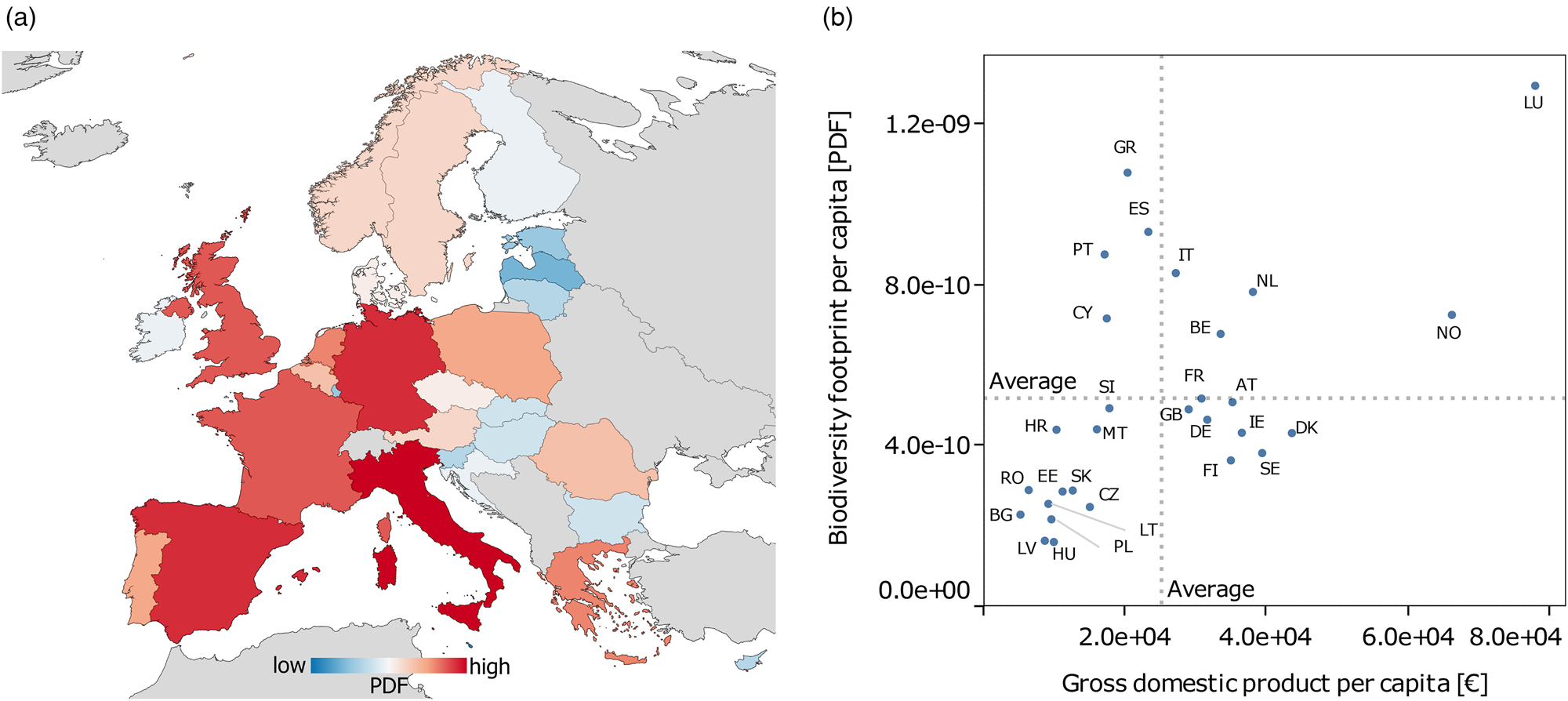
In absolute terms, the countries responsible for the highest absolute biodiversity losses are by far Europe's large economies, i.e. Germany, Italy, Spain, France and the UK (Figure 1a). On a per capita basis, however, results are less unequivocal – which is also linked to the choice of impact methodology (Figures S7 and S8). More specifically, LC-IMPACT footprints exhibit a twofold pattern: Mediterranean countries such as Greece and Spain, and those with high per-capita GDP such as Luxembourg have the highest per capita biodiversity impacts (Figure 1b). Following the ReCiPe-methodology, however, no clear pattern can be identified for the most impactful countries on the per-capita scale, except for the two top GDP-per-capita nations Norway and Luxembourg leading the list, while it is East-European countries that have the lowest impacts.
LC-IMPACT biodiversity footprints of EU28 + Norway for 2010. (a) shows absolute national biodiversity footprints and (b) shows per capita biodiversity footprints against the per capita GDP per country. See Table S2 for country abbreviations. Countries other than EU28 + Norway are grey-shaded in (a). The dotted lines in (b) represent the per capita footprint and GDP averages (see Tables S14–S16).
The major driver of biodiversity losses is found to be land use. On average across Europe and fairly stable over the years with not more than 4% deviation (the per-country fluctuations have a wider range), land use as a mechanism is responsible for 63–81% maximum (from ReCiPe and LC-IMPACT, respectively; cf. country levels in Tables S20–S21) of the total biodiversity impact footprint in 2010. The next largest mechanisms are global warming and terrestrial acidification, at roughly 20% and 13% for ReCiPe and 9% and 8% for LC-IMPACT, all in 2010.
3.2. Trade related biodiversity losses
European countries have a significant share of environmental pressures and impacts embodied in trade. For brevity, the following results only refer to the LC-IMPACT footprints. Only about 31% of species losses attributable to total European household consumption are sourced from inside Europe, and all countries are net importers of biodiversity footprints, i.e. the species losses associated with the import of goods to the respective country are greater than those linked to its exports (Table S22). Around 40% of the exports of European countries stay within European boundaries. With the exceptions of Bulgaria, Spain, Greece and Croatia, all of which have a higher domestic impact, all European countries have more imported biodiversity losses than domestically sourced ones (Table S23). The import shares are highest for countries with high GDP per capita, namely Norway (95%), Belgium (97%), the Netherlands (98%) and Luxembourg (99%). For the remaining countries, import shares range typically from 50 to 70%. While most countries had even higher import shares in 2005, a few countries, most prominently eastern European ones, showed decreases in their domestic share from 2005 to 2010. The most noteworthy change during this period is, however, Italy's drop in import shares from 74 to 57%. A country's characteristic of being a net-importer of species losses is, with slight fluctuations, also reflected in the individual impact categories.
European countries clearly differ as to where the sources of their imported biodiversity losses lie. For instance, RoW Africa is the largest contributor to France's footprint with about 23%, whereas only 5% of species losses attributable to Bulgaria's household consumption are sourced from RoW Africa. Overall, the largest sources for biodiversity footprints embodied in international trade for European consumption are RoW Africa (12.1%), RoW America (14.2%) and Spain (12.7%), followed by Italy (8.8%), RoW Asia and Pacific (6.7%) and France (5.4%) (Figure 2). The largest absolute domestic flows of species losses are in Spain and Italy (Figures S9 and S10).
Total global biodiversity losses due to European household consumption in 2010, measured in PDF. The panel in the bottom-left corner shows the biodiversity losses in Europe due to land use for annual crops (cf. Figure 4), associated with European household consumption in 2010. The countries are grouped according to the EXIOBASE-classification.

3.3. The effect of urbanization
Both LC-IMPACT and ReCiPe biodiversity footprints in cities are, in absolute terms, higher than in towns or rural areas. If not indicated differently, the following results refer to the LC-IMPACT footprints. On the European level, more than 50% of total ecosystem damage is caused by household consumption of urban populations. Towns are accountable for about 27%, and the remainder is due to final demand in rural areas. This same pattern can, however, be observed only across a few individual countries, mainly the ones with high absolute footprints, i.e. Italy, the UK and Germany. While urban areas have the highest share in total biodiversity losses in most countries, e.g. Cyprus (60%), Finland (65%) or the UK (61%), rural areas are often the ones with the second highest contribution, e.g. in Austria (37%), France (37%) or Ireland (34%). But there are also countries where the highest biodiversity footprints are borne by people living in the countryside, for instance, in Hungary, Sweden and Slovakia with between 40 and 60%. The strongest signal of urban biodiversity footprints is in Malta with 93%. In Latvia, cities and rural areas are responsible for about 50% of the national biodiversity footprint each.
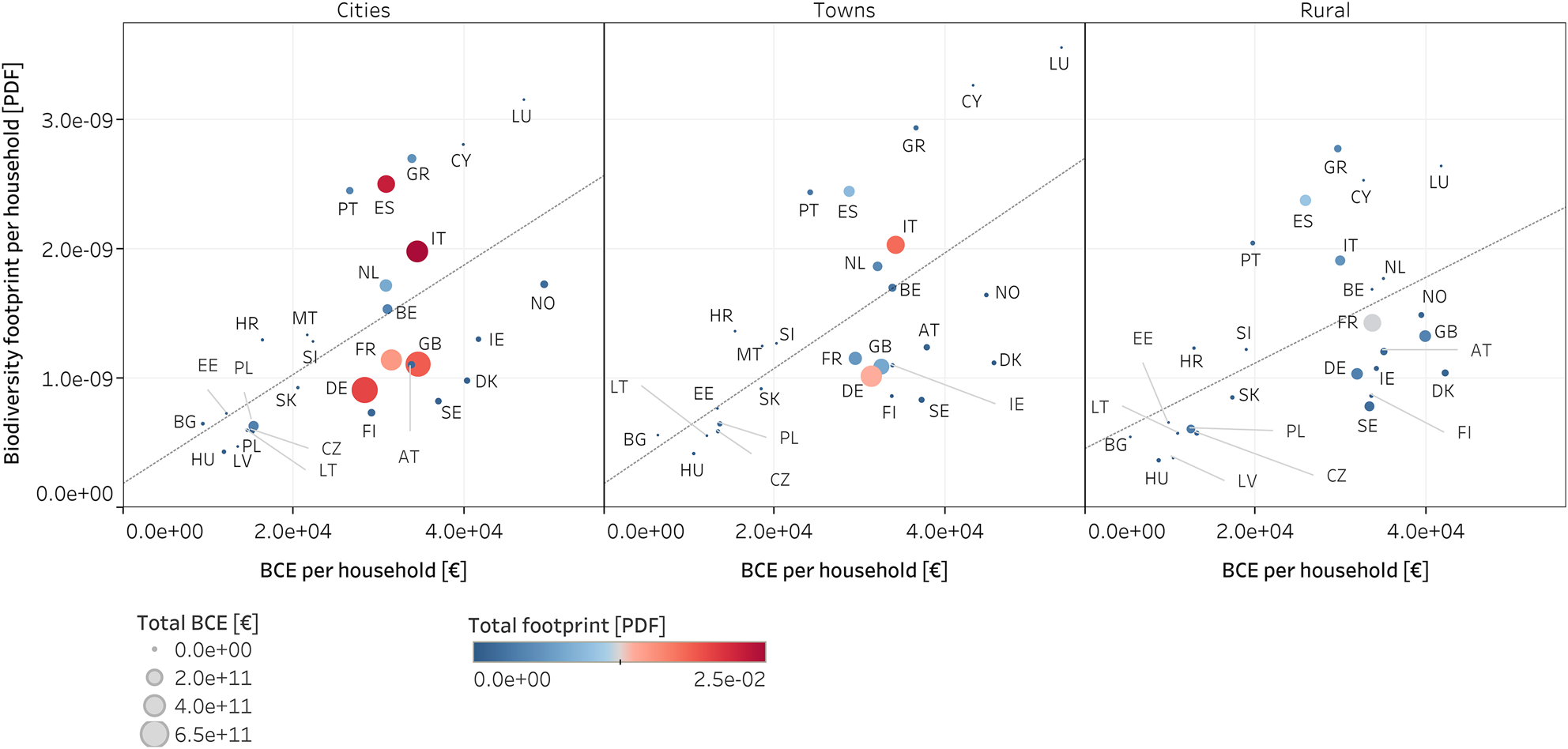
Both on the per capita as well as per household levels, differences are, however less distinct. A city resident in Europe is accountable for about 5% higher biodiversity losses than the average European citizen, whereas suburban residents have biodiversity footprints that are only 2% higher, and rural residents have footprints that are 12% lower than average.Footnote ii While this is also the case in most countries, some exceptions do exist: in smaller economies such as Bulgaria, Croatia, Hungary or Ireland, the per capita biodiversity footprint distribution shares of urban populations are relatively higher than the European city distribution share. Conversely, rural populations in, amongst others, France and the UK have a stronger per capita impact on biodiversity compared with the average European city resident. While the biodiversity footprints of Norwegians living in any area type are highest in direct comparison across Europe according to the ReCiPe assessment, this applies to Luxembourg citizens in cities and towns as well as Greek rural residents when applying the LC-IMPACT methodology. For a comparison on the per household level, see Figure 3 as well as Figure S11. In either case, biodiversity losses disaggregated by degree of urbanization correspond to the balanced consumer expenditure, i.e. the higher the expenditure, the higher the footprint.
LC-IMPACT biodiversity footprints disaggregated by degrees of urbanisation for 2010. The axes show the biodiversity footprints and balanced consumer expenditure (BCE) per household per country; circle sizes indicate the total balanced consumer expenditure (small – low, big – high); colouring denotes the total biodiversity footprint (blue – low, red – high). The dotted lines are linear trend lines. See also Figure S11 and Tables S24–S25.
The relative breakdown of impact categories per degree of urbanization in a country differs only slightly, i.e. max. 3%, compared with national averages, both in absolute and per capita terms for all countries. That is, for instance, Germany's share of land use in all area types of around 78% in 2010 is about the same as in its national average. However, comparing the contributions per impact category across the degrees of urbanization shows that in most countries and impact categories city residents are more accountable than people living in towns or in the countryside. Scaling this to the European level, urban citizens carry higher weights in the categories of land occupation and water stress (up to 7% higher than the average per capita footprint per impact category), whereas people living in towns have higher footprints than the average European citizen regarding ecosystem damage related to emissions of, for example, fossil methane and sulphur hexafluoride (Tables S26–S28).
Land use prevails as the highest contributor to the overall biodiversity footprint across cities, towns and rural areas. While the absolute land use for annual crops, intensive forestry and pastures is of similar magnitude, it is annual crops that have the greatest impact (Figures 4 and S12). The ratios of urbanization degrees within each land use type are comparable to the total.
Differences across urbanization degrees and the importance of land use. a) shows the absolute biodiversity footprint per area type, indicating the share of land use; (b) shows land use pressure and impact disaggregated by land use type and the share of each degree of urbanization. For Ireland, Malta, the Netherlands and Sweden, no disaggregated 2005 data were available; therefore, 2010 data were used for these countries. Romania is not included due to a lack of data in both years.

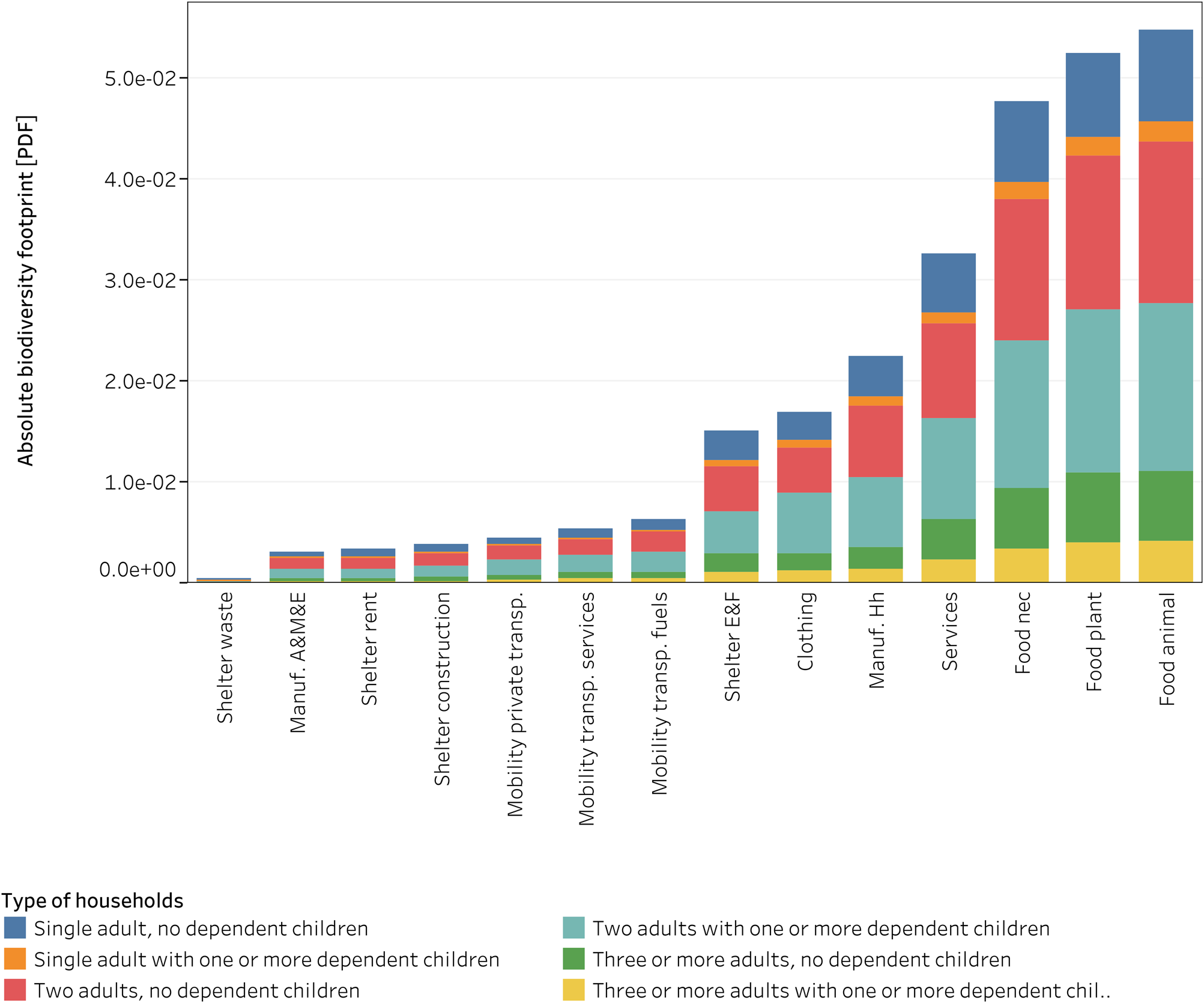
Since land use is the most important mechanism driving biodiversity impact, land-intensive products are seen to be the most intensive product-level drivers (Figure 5). Food, services (including restaurants, and other services, which buy food as part of their business), clothing, and to a lesser extent, building materials, are the largest product drivers. We also observe impacts through water stress, chemical pollution (including from manufacturing and burning gasoline), and eutrophication impacts (including from the production of meat and leather), though these categories are minor (see spreadsheet appendix for full detail). The relative contributions from the various product groups do not change significantly across household types (Figures 5 and S13–S15). In per capita terms, households consisting of three or more adults without dependents are the ones with the highest overall footprints. In absolute terms, the major contribution per sector comes from households with two adults (see also Table S29).
LC-IMPACT biodiversity footprint per sector for 2010. The left axis describes the absolute European footprint disaggregated by types of households. The sector grouping was established using a concordance matrix (EXIOBASE sector to sector group) from Ivanova et al. (Reference Ivanova, Vita, Steen-Olsen, Stadler, Melo, Wood and Hertwich2017). Colouring denotes the distinct types of households. The full sector group names can be found in Table S30.
3.4. Income as a determinant for impact
While we find that both per capita and absolute biodiversity footprints increased with increasing income in 2010, no such development can be observed for 2005 (Figure 6 as well as Figure S16). More specifically, the absolute footprint still follows the former pattern, although less pronounced than in 2010, but per capita biodiversity impacts associated with final demand in low income quintiles are considerably higher in 2005. The per capita footprints attributable to Europe's second income quintile even exceed the footprint attributable to the fifth income quintile in 2005.
LC-IMPACT biodiversity footprints disaggregated by income quintiles. a) shows 2005 footprints, (b) shows 2010 footprints. The primary axes describe per capita footprints, whereas the secondary axes scale absolute footprints (black line). Colouring denotes different impact categories. Note that the 2005 footprints do not include the contribution of Ireland and Sweden due to missing data; replacing these with 2010 data as in Figure 3 is not possible due to the nature of the data. No data on income quintiles in Norway were available in either year.

However, when normalizing the biodiversity footprints against the respective balanced consumer expenditure, the patterns for both years resemble one another (Figure S17). Across both reference years and all European countries, these normalized footprints decrease, the higher the income. Independent of the normalization procedure, land use accounts in both years and across all income quintiles for most of the biodiversity footprint, ranging from around 80% (62% for ReCiPe) for quintile five in 2010 to slightly above 84% (65% for ReCiPe) for the first quintile in 2005.
4. Discussion and conclusion
A decrease in both absolute and per capita footprints in the period 2005–2010 was identified for the European total and most individual countries. Because the GDPs of most European countries increased at the same time, a decoupling of biodiversity impacts from affluence is indicated. With only two reference years that cover the financial crisis, more evidence is needed to state that this is a longer-term trend. Differences within each country exist across impact categories as well as within each impact category across countries.
The ranking of national biodiversity footprints depends largely on the chosen impact assessment methodology. That is, although ReCiPe and LC-IMPACT footprints show a similar overall pattern, they differ in detail across European countries, with location and per-capita wealth being the dominating factors for both footprint types. Already Verones et al. (Reference Verones, Moran, Stadler, Kanemoto and Wood2017) showed the interlinkage between the size of biodiversity footprints and income levels and that biodiversity losses are influenced by levels of endemism, species richness and their vulnerability in richer countries. Deviations between the footprint types can be attributed to their different nature and the underlying methodology. A brief discussion on fundamental implications regarding the choice of impact methodology is provided in SI11.
While urbanization has a major influence on the absolute biodiversity footprints of countries, it is less pronounced on the per capita and per household levels. The high share of species losses attributable to city residents on a national level is mainly due to the size of urban populations in Europe. In times of urban sprawl, related social and demographic changes, as well as society's high impact on the planet, sustainable urban development and regional planning become more important than ever before. Moreover, it can be observed that, with few exceptions, absolute biodiversity footprints in each degree of urbanization follow the magnitude of the total GDP and the population size across all countries and all impact categories. The variation of national per capita footprints across all area types and all impact categories, however, has a less clear signal. Nonetheless, we find that both absolute and per household footprints are correlated to GDP and balanced consumer expenditure across all degrees of urbanization.
In relation to that, it was shown that income is a major driver of biodiversity losses due to household final demand on absolute national averages and for the whole of Europe. That is, the higher the income, the higher the footprint. This is in alignment with studies explaining the magnitude of environmental pressures with both expenditure and income (Jones & Kammen Reference Jones and Kammen2014; Chancel & Piketty Reference Chancel and Piketty2015; Ivanova et al. Reference Ivanova, Stadler, Steen-Olsen, Wood, Vita, Tukker and Hertwich2016, Reference Ivanova, Vita, Steen-Olsen, Stadler, Melo, Wood and Hertwich2017; Steen-Olsen et al. Reference Steen-Olsen, Wood and Hertwich2016). While that holds also for the 2010 per capita level, per capita footprints in 2005 appear to be decoupled from income. Such variation can, however, be explained by expenditure patterns. That is, per capita footprints in proportion to per capita expenditure decrease from low to high income for both reference years. While the raw results of the income-footprint nexus extend the finding of non-saturation regarding environmental pressures with increasing wealth by Hertwich & Peters (Reference Hertwich and Peters2009) and others, the normalized results rather corroborate the controversial hypothesis of the environmental Kuznets curve (Stern Reference Stern2004). A definitive, generalized answer on the role of income across both, absolute and per capita, levels is therefore not possible, but differentiation is necessary.
In line with other biodiversity footprint studies (Verones et al. Reference Verones, Moran, Stadler, Kanemoto and Wood2017; Wilting et al. Reference Wilting, Schipper, Bakkenes, Meijer and Huijbregts2017), land use was found to be the major contributor to biodiversity losses. Land use, in turn, was shown to be mainly driven by the demand for agricultural food products, which is in accordance with Kitzes et al. (Reference Kitzes, Berlow, Conlisk, Erb, Iha, Martinez and Harte2017) and Wilting et al. (Reference Wilting, Schipper, Bakkenes, Meijer and Huijbregts2017). The role of food commodities was also recently highlighted by Castellani et al. (Reference Castellani, Beylot and Sala2019), Crenna et al. (Reference Crenna, Sinkko and Sala2019) and Marques et al. (Reference Marques, Martins, Kastner, Plutzar, Theurl, Eisenmenger and Pereira2019). The impacts of this demand and other European consumption are, however, to a large extent imposed on countries in other regions of the world, whereas domestically caused species losses are considerably lower. Additionally, it must be noted that climate change, on both a local and global level, could take a larger toll on biodiversity in the future given the dramatically increasing concentrations of greenhouse gases in the atmosphere. Moreover, we observe that Europe is a net-importer of biodiversity losses, a result that aligns with earlier studies on both environmental pressures and impacts (Lenzen et al. Reference Lenzen, Moran, Kanemoto, Foran, Lobefaro and Geschke2012; Giljum et al. Reference Giljum, Wieland, Lutter, Bruckner, Wood, Tukker and Stadler2016; Lutter et al. Reference Lutter, Pfister, Giljum, Wieland and Mutel2016; Kitzes et al. Reference Kitzes, Berlow, Conlisk, Erb, Iha, Martinez and Harte2017; Wilting et al. Reference Wilting, Schipper, Bakkenes, Meijer and Huijbregts2017; Wood et al. Reference Wood, Stadler, Simas, Bulavskaya, Giljum, Lutter and Tukker2018). Such an imbalance may be a source for ethical demur and raises the question of producer vs consumer responsibility (Lenzen et al. Reference Lenzen, Murray, Sack and Wiedmann2007) – an answer to which shall not be attempted here.
Additionally, the impact distribution is sector dependent. Therefore, directed intervention via policy instruments such as taxes on certain goods for curbing further ecosystem damage associated with household consumption is not straightforward. With the highest biodiversity losses embodied in agricultural products, the discourse on the role of food and non-food commodities must be widened to reach multiple stakeholders including the public, the scientific community and policymakers. Differences regarding the environmental performance of producers of agricultural products as well as the effectiveness of environmental policies and regulations could not be analysed here but should be addressed in future research. Additionally, our model could be combined with the approach by Froemelt et al. (Reference Froemelt, Dürrenmatt and Hellweg2018) for gaining more insights into consumption patterns of individual countries.
Given that urbanization is expected to increase and that more countries strive for ever more wealth, stronger impacts on the environment would be the consequence, both domestically and, even more so, abroad. Therefore, political action is crucial – yet, not only that: the responsibility of the individual is also asked for to avert further negative environmental corollaries of household consumption. Be it environmental laws and regulations, or just the decision of the individual to abstain from, for instance, meat consumption and do without the extra cup of coffee in the morning, both behavioural and structural changes could reduce humanity's footprint on the planet.
Supplementary material
To view supplementary material for this article, please visit https://doi.org/10.1017/sus.2019.23
Acknowledgements
The authors would like to thank the editor Xuemei Bai and two anonymous reviewers for their constructive suggestions improving the quality of the manuscript.
Author contributions
MK led the work. RW and DM designed the research and assisted with the paper and implementation. AT assisted with the consumer expenditure data. FV contributed the LCIA models and biodiversity metric expertise.
Financial support
This work was supported by the Norwegian Research Council (grant # 255483/E50).
Conflict of interest
The authors declare they have no conflict of interest.


 Open access