2. Related works

Several semi-automated and automated methods exist for surface and bottom tracking in radar images (Crandall and others, Reference Crandall, Fox and Paden2012; Lee and others, Reference Lee, Mitchell, Crandall and Fox2014, Mitchell and others; Mitchell and others Reference Mitchell, Crandall, Fox and Paden2013a; Reference Mitchell, Crandall, Fox, Rahnemoonfar and Paden2013b, Rahnemoonfar and others; Rahnemoonfar and others; Rahnemoonfar and others Reference Rahnemoonfar, Yari and Fox2016; Reference Rahnemoonfar, Abbassi, Paden and Fox2017a; Reference Rahnemoonfar, Fox, Yari and Paden2017b). As mentioned above, tracking internal layers is a significantly different and generally more difficult task because of the large number of layers in close proximity and the number of layers is unknown. Panton (Reference Panton2014) describes a semi-automatic method for tracing internal layers in radio echograms based on the Viterbi algorithm. The algorithm was tested on a relatively short 423 line-km radar depth sounder dataset and showed promising results, but still relied on the use of manually labeled seed points. MacGregor and others (Reference MacGregor2015b) transform the images so that the layers are flattened by using an internal layer slope field. The flattened layers are then tracked with a simple snake algorithm that tracks the peak power column to column. The simple algorithm works well when the layers are contiguous (no gaps in the layer) and flat, but still requires some user input to seed the snake algorithm. Two methods are used to generate the slope fields. One is a phase coherent method that uses a matched filter for specular layer scattering to estimate the layer slopes. Although this algorithm works well for specular (coherent) layers, some layers, including those typically detected by the Snow Radar, are not coherent scatterers and therefore an algorithm relying on phase coherence from column to column is not likely to work well. MacGregor and others (Reference MacGregor2015b) also use a method that works on incoherent scatterers based on Sime and others (Reference Sime, Hindmarsh and Corr2011) which uses filtering, thresholding and feature extraction to estimate layer slopes from the slopes of the features. Using this process of flattening and the simple snake algorithm, the task took a couple years to complete and although many layers were tracked in the imagery that was analyzed, there are still untraced layers due to time limitations. de Paul Onana and others (Reference de Paul Onana, Koenig, Ruth, Studinger and Harbeck2014) describe an algorithm that relies on surface flattening, filtering for horizontal features and automated peak finding to seed layers. The method is largely automated, but still required a manual step to index layers. The algorithm is generally not able to track all human-detectable layers and especially struggles with layers with larger slopes relative to the surface. Carrer and Bruzzone (Reference Carrer and Bruzzone2016) present a locally applied Viterbi algorithm which works well with ice sounder data collected on the Mars north polar ice cap. This method is fully automated after an initial training phase. To the best of our knowledge, there are no internal layer tracking algorithms that utilize deep learning techniques.

Most traditional approaches to edge and contour detection problems fundamentally make use of image spatial derivative operators. Since the derivative operators possess high-pass characteristics of the image, they can effectively enhance edges in an image and make them more pronounced. The downfall of the derivative operator, however, is that it is susceptible to noise. Now in order to reduce the sensitivity of derivative operators to noise, one can employ regularization filters, such as a Gaussian filter. Traditional edge detectors, such as Canny (Reference Canny1986) and Marr and Hildreth (Reference Marr and Hildreth1980), are prime examples of edge detectors that combine regularization with derivative operators.

Traditional edge detection techniques are based on hand-crafted feature engineering and cannot be applied to a large-scale dataset. In recent years, there have been several deep learning techniques for contour detection in optical imagery (Shen and others, Reference Shen, Wang, Wang, Bai and Zhang2015; Bertasius and others, Reference Bertasius, Shi and Torresani2015; Xie and Tu, Reference Xie and Tu2015; Liu and Lew, Reference Liu and Lew2016; Liu and others, Reference Liu, Cheng, Hu, Wang and Bai2017). The pioneering deep learning techniques use fully connected layers so they are limited to images with fixed sizes. However, recent deep learning techniques focus more on fully convolutional networks and multi-scale features to extract both local and global information from the image. There are two main types of network structures to generate multi-scale features. The primary option is to resize the original image and pass it to the network and then combine the results. The more intelligent way is to extract multi-scale features through the hidden layers in a deep neural network; Holistically nested Edge Detection (HED) (Xie and Tu, Reference Xie and Tu2015), Relaxed Deep Supervision (RDS) (Liu and Lew, Reference Liu and Lew2016) and Richer Convolutional Features (RCF) (Liu and others, Reference Liu, Cheng, Hu, Wang and Bai2017) are among the second approach. The early layers in the deep neural network extract the local and detailed information while the last layers extract the global information. Since our radar data are noisy, we have implemented a multi-scale edge detection technique which can extract both local and global information and at the same time address the noise issue.

3. Dataset

We analyze Snow Radar (Rodriguez-Morales and others, Reference Rodriguez-Morales2018) images produced by the Center for Remote Sensing of Ice Sheets for NASA Operation IceBridge. The Snow Radar is a profiling instrument which produces vertical sounding images of snow layers over ice sheets and ice caps. The radar signal is sensitive to shallow annual snow density changes that occur in the top few tens of meters of ice due to the seasonal transitions from summer to winter; this density change results in a snow permittivity change at the interface that scatters the radar signal which is measured by the radar's receiver. For training our network we used the output of semi-supervised layer tracking from de Paul Onana and others (Reference de Paul Onana, Koenig, Ruth, Studinger and Harbeck2014). The layers were quality controlled by a human analyst for Koenig and others (Reference Koenig2016). This included correcting layers, adding missing layers and deleting layers which were in error or too difficult to interpret with sufficient confidence as annual layers. While the tracking is largely comprehensive, there are some layers that are not tracked. In some cases, layers were removed if they were thought to be caused by something other than the annual layer indicating the transition from summer to fall. In other cases, layers that could be tracked by the analyst may not have been due to perceived value in tracking the layer, difficulty to track the layer in question, and time constraints to complete the work. In total, we use 93700 line-km of images collected over Greenland during the 2012 field season that were tracked by Koenig and others (Reference Koenig2016). The images we use have the same preprocessing steps applied as described in Koenig and others (Reference Koenig2016) which includes filtering, decimation and surface flattening. The filtering operates on incoherent power detected data, helps to denoise the data and is analagous to multilooking. The 2012 field season includes coverage of most of Greenland and the dataset is well representative of Snow Radar image variability.

In one of our experiments we used synthetic data for training. The synthetic dataset models the layers as the superposition of many point targets. The scattered signal from each point target is represented by a weighted sinc function. The weight for each sinc function is a complex Gaussian random variable. The thickness of each layer represents the separation between interfaces and is generated by a smoothed Gaussian random process. The mean thickness or separation decreases slightly with depth and starts at 75 pixels for the first layer. The standard deviation of the random process is 10% of the mean thickness. The depth of a layer results from the summation of the thickness of the layer and all layers above it. For each column of the image, the scattered signal for each layer is created by summing the contribution of 100 point targets spread slightly in range. The spreading in range is generated from the summation of a Gaussian distribution and an exponential distribution to simulate the spread of the scatterers over several range bins as well as the backscatter fall-off from each layer as a function of cross-track incidence angle. The mean signal power of each layer follows an exponential decay with depth so that deeper layers have weaker signals on average. The images are power detected, filtered and surface flattened similar to the real radar data. The various parameters used to generate the data are chosen manually to create images that are similar to the Snow Radar data, but no effort is made to precisely match the Snow Radar image statistics. The synthetic images represent a first-order attempt and although they share some resemblance to the Snow Radar images, they are easily distinguished from them.

4. Convolutional neural networks

Convolutional neural networks (CNN) are a class of deep neural networks that mainly focus on analyzing imagery. CNN comprise various convolutional and pooling (subsampling) layers that can be compared to the visual system of humans. Generally, image data are fed into the network that constitutes an input layer and produces a vector of reasonably distinct features associated to object classes. From input to output layers there are many hidden layers including convolution layers, pooling layers and fully connected layers.

To provide understanding of the activities at each layer in a neural network, some explanation of the various processes is provided below.

Convolution: The main building block of a CNN is a convolutional layer. The parameters of this layer include a set of learnable filters (or kernels), which have a small receptive field, but spread through the full depth of the input. Every filter is convolved along the width and height of the input volume and produces a two-dimensional feature vector of that filter. All the feature vectors generated through different filters are stacked together along the depth dimension to form an output volume of the convolution layer (Bustince and others, Reference Bustince, Barrenechea, Pagola and Fernández2009). The input to the layer is represented as a tensor and is used in the convolution operation along with the filter kernel. In order to control the number of parameters in convolutional layers, the parameters are shared.

Activation: Activation functions are used to normalize outputs of a neural network. A common activation is the Rectified Linear Unit, also known as ReLU. This function simply calculates the maximum of zero and the output of the neuron. A variation of this activation function is known as the Leaky ReLU. Here, the function calculates the maximum of the output of the neuron and a small constant value multiplied to the output.

Pooling: The pooling layer is a form of non-linear down-sampling applied to reduce the size of the feature vectors generated through convolution. The idea is to reduce the number of parameters and the computation required and therefore to control overfitting. Several non-linear functions are available to perform pooling such as max pooling, min pooling and average pooling. Max pooling reports the maximum output within a rectangular neighborhood. Average pooling reports the average output of a rectangular neighborhood.The most common approach to apply pooling is between successive convolution layers.

Fully connected layer: After a series of convolutional and pooling layers, finally the abstract-level reasoning is performed using a fully connected layer. In this layer, neurons have full connections to all the activation outputs in the previous layer, similar to classical neural networks. There can be many fully connected layers before the final output layer.

Regularization: A common way to prevent over-fitting for a network is to employ the concept of dropout. In this method, neurons are randomly ignored in a layer. This essentially makes the network into an ensemble of many possible subnets. Following this method, there is less chance that one neuron will ever be relied upon too heavily.

Classification: For every possible class the network is trained to identify, there will be an output neuron. In order for these outputs to follow a probability distribution, a softmax function is applied after the final output of the network. When softmax is used, all the probabilities will add up to one.

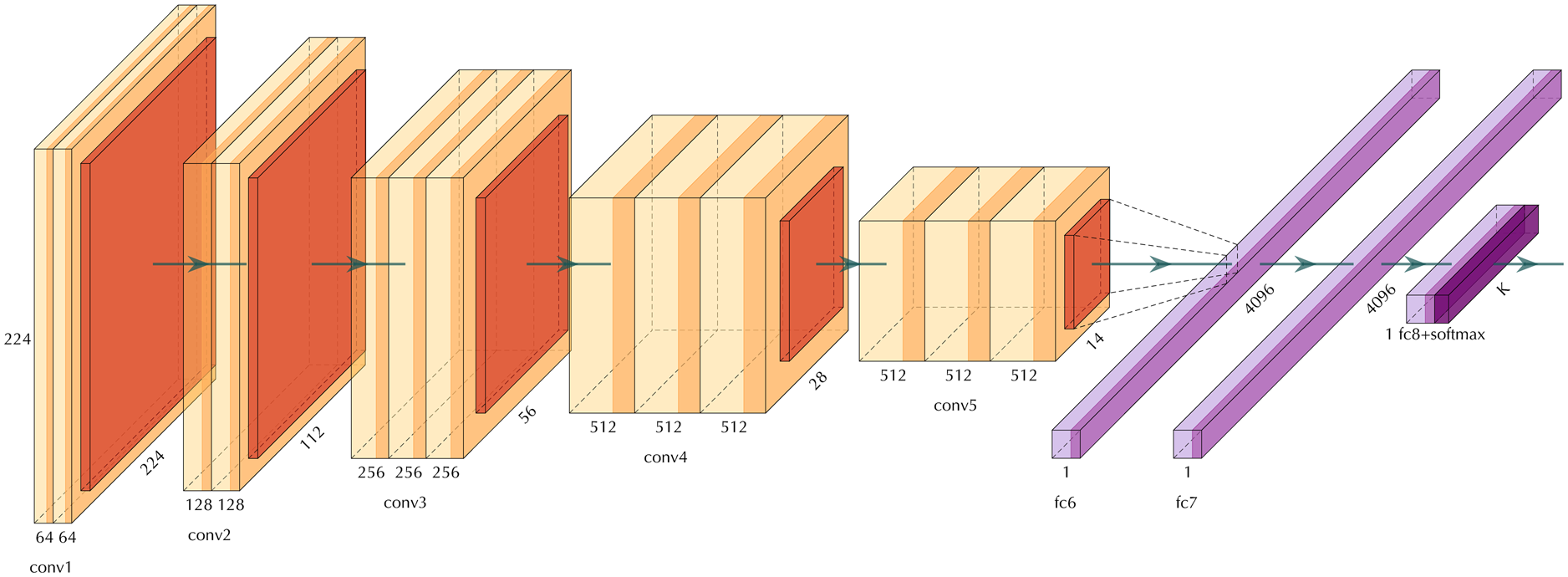
Several deep neural network architectures such as AlexNet (Krizhevsky and others, Reference Krizhevsky, Sutskever and Hinton2012b), VGG-net (Simonyan and Zisserman, Reference Simonyan and Zisserman2015) GoogLeNet (Szegedy and others, Reference Szegedy2015b) and Resnet (He and others, Reference He, Zhang, Ren and Sun2016) have made such significant contributions to the field that they have become widely known standards. AlexNet was the pioneering deep neural network architecture that won the ImageNet Large Scale Visual Recognition Challenge (Deng and others, Reference Deng2009) in 2012. VGGNet won the challenge in 2014 along with GoogLeNet. The VGGNet architecture is depicted in Figure 1. As you can see in this figure, the building blocks of VGGNet includes the convolution, pooling and fully connected layers that were explained previously.

Fig. 1.

The architecture of VGGNet. The orange layers show convolution layers, the red layers are pooling layers, and violet layers are fully connected layers.

5. Methodology

In this research, we employ a multi-scale learning model to trace snow boundary layers for real radar data. Multi-scale deep learning models are characterized by their use of the so-called side-output. Figure 2 provides an example of a multi-scale learning model where several side-outputs at different scales are extracted. Each side-output layer is associated with a classifier and an objective function. The ensemble of the side-outputs generates a fuse prediction at the final stage and is associated with another objective function. Therefore, the model is equipped with several objective functions and learning components at different scales. In terms of the architecture, we base our construct on an existing architecture to take advantage of pre-trained parameters. This approach is particularly helpful for transfer learning purposes.The multi-scale architecture introduced in (Xie and Tu, Reference Xie and Tu2015) takes the VGGNet (Fig. 1) as its parent architecture. Each of the first five blocks of the VGGNet follows the same architecture. It consists of a consecutive number of convolutional layers and activations, followed by a max-polling layer. The max-pooling layer will rescale the image based on the size of the max-pooling feature map. For a two by two max-pooling size, the size of the image will reduce to half the original size in each dimension.

Fig. 2.

The architecture of a multi-scale convolutional neural network. The orange layers show convolution layers, the red layers are pooling layers, and the blue layer is the fused layer.

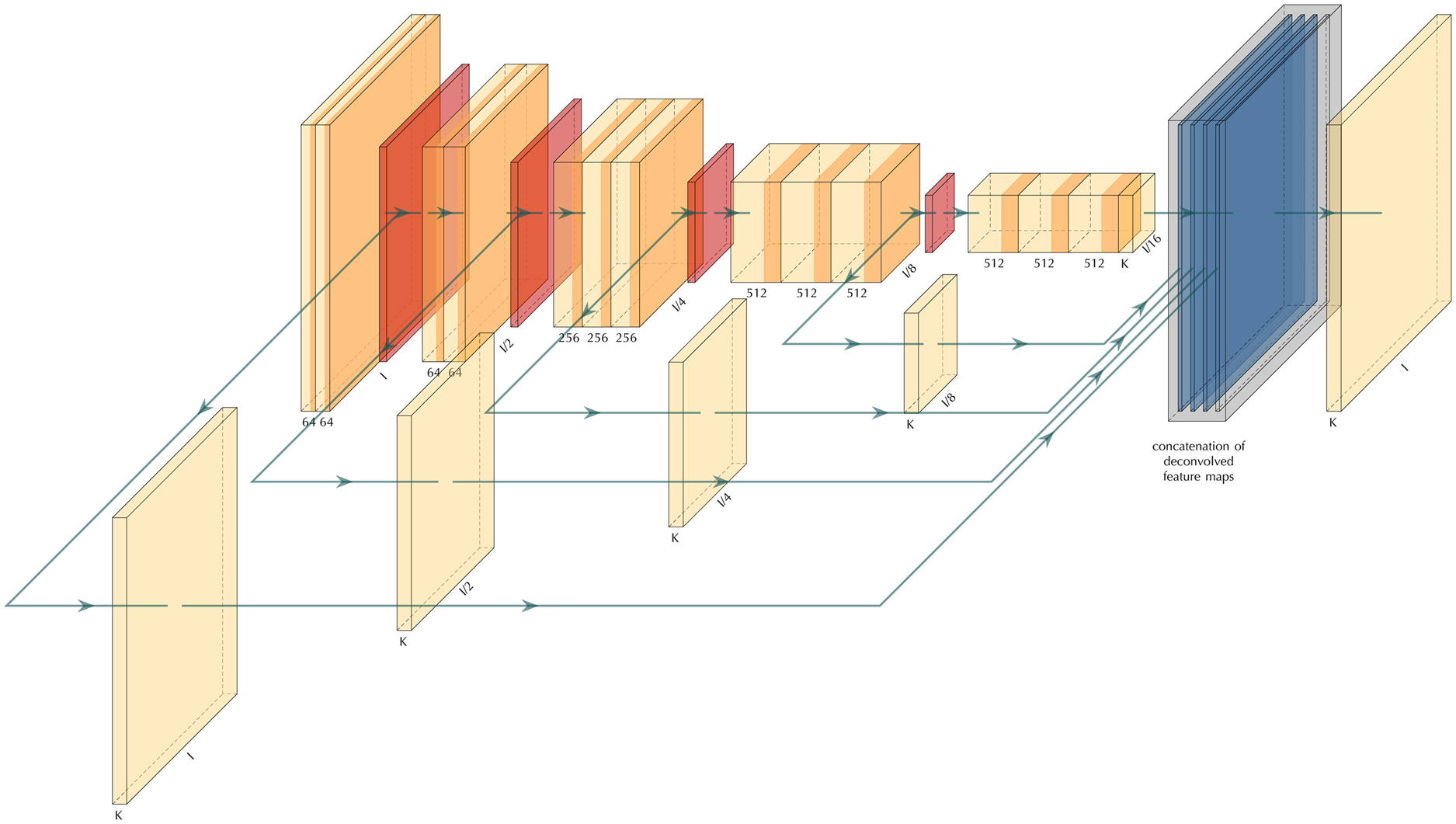
Following the HED model of Xie and Tu (Reference Xie and Tu2015), we extract the side-outputs right before the max-pooling layers and drop the final fully connected layers of the VGGNet. This way, we end up with five side-outputs which we will fuse at the end to produce the final prediction. As mentioned previously, in addition to our final objective function, we have five other objective functions associated with each side-output. Moreover, the fuse weights are part of the learnable parameters; therefore, the model tries to get the best way of fusing the side-outputs as well. Another advantage of this approach is that it facilitates using the various sized input images.

In mathematical terms, we denote the original data in our training dataset by $X = \lcub X_{n}\colon n = 1\dots N\rcub$, where $N$ is the size of the dataset; we also denote the corresponding boundary data by $Y = \lcub Y_{n}\colon n = 1\dots N\rcub$. The HED model pulls out $M$ side-outputs by $Y_{n}^{\lpar m\rpar }$for $m = 1\dots M$, and a final output of the weighted-fusion layer, denoted by $\widetilde {Y}_{n}$. The model includes $M$ image-level loss functions at each side-output layer, denoted by $\ell _{m}$ for side-output $m$, and a loss function at the fusion layer, denoted by $\ell _{{\rm f}}$. We denote all parameters of the classifier associated with the $m^{{\rm th}}$ side-output by $\theta _{m}$. Then the loss function $\ell _{m}$ is defined as a class-balanced cross-entropy function as in Eqn (1):

(1)$$\eqalign{\ell_{m} = \ell_{m}\lpar \theta_{0}\comma\; \theta_{m}\rpar = & -\beta\sum\limits_{\,j\in Y^{ + }}\log \lpar Pr\lpar y_{\,j} = 1\vert X\semicolon\; \theta_{0}\comma\; \theta_{m}\rpar \rpar \cr & - \lpar 1-\beta\rpar \sum\limits_{\,j\in Y_{-}}\log \lpar Pr\lpar y_{\,j} = 0\vert X\semicolon\; \theta_{0}\comma\; \theta_{m}\rpar \rpar }$$

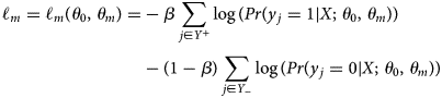
where $\theta _{0}$ represents all other standard network layer parameters, $Y_{-}$and $Y_{ + }$ are the edge and non-edge labels respectively and $\beta = \vert Y_{-}\vert /\vert Y\vert$. The loss function for the final fusion layer is defined by

(2)$$\ell_f\lpar \theta\comma\; w\rpar = CE\lpar Y\comma\; \widetilde{Y}\rpar \comma\; $$

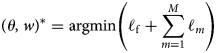
where $CE$ is a cross-entropy loss function that measures dissimilarities of the fused prediction and the ground truth label; $\theta = \lpar \theta _{0}\comma\; \, \theta _{1}\comma\; \, \dots \comma\; \, \theta _{m}\rpar$, and $w = \lpar w_{1}\comma\; \, \dots \comma\; \, w_{m}\rpar$ represents the fusion weights. Putting everything together, the goal is to minimize the following objective function via standard (back-propagation) stochastic gradient descent:

(3)$$\lpar \theta\comma\; w\rpar ^{\ast } = {\rm argmin}\left(\ell_{\rm f} + \sum_{m = 1}^M \ell_m\right)$$

We use a mini-batch gradient descent that computes the gradient of the cost function with respect to the parameters $\theta$ for the entire training dataset: $\theta = \theta -\eta \nabla _{\theta }{\cal L}\lpar \theta \comma\; \, x^{I}\comma\; \, y^{I}\rpar$. Here we used the symbol $\theta$ for all parameters. This minimization approach is based on Nesterov accelerated gradient technique as discussed in Sutskever and others (Reference Sutskever, Martens, Dahl and Hinton2013):

(4)$$v_{t} = \mu v_{t-1} + \eta\nabla_{\theta}{\cal L}\lpar \theta_{t-1}-\mu v_{t-1}\rpar \comma\; \quad \theta_{t} = \theta_{t-1}-v_{t}$$

where $\mu \in \lsqb 0\comma\; \, 1\rsqb$ is the momentum and $\eta \gt 0$ is the learning rate, see Sutskever and others (Reference Sutskever, Martens, Dahl and Hinton2013).

Input images are not resized for training or testing. Since we get the side-outputs right before applying the max pooling, the size of the first output matches with the original input size. But after applying the max pooling, the second side-output is half the size of the first side-output; likewise, each subsequent side-output is going to be half the size of the previous side-output. Therefore, each side-output is generated at a different scale.

In the training process, we have used the following parameters $\gamma = 0.1$, learning rate $\eta = 10^{-6}$ and the momentum $\mu = 0.9$. We have also used weight decay rate of $2\times 10^{-4}$.

6. Experimental results

In this section we report our experimental results on our dataset. We refer to our real dataset of ice radar imagery, as ICE2012, which consists of 2360 training images and 260 test images. We refer to our synthetic dataset as SYNT_ICE, which consists of one thousand synthetic images, and use it for the training phase only. For pre-training and transfer learning models, we use the benchmark BSDS500 dataset (Martin and others, Reference Martin, Fowlkes, Tal and Malik2001). We present the results of three main experiments that we carried out.

1. (1) BSDS: We trained our model on augmented BSDS500.

2. (2) SYNT: We trained the model on the synthetic ice dataset (SYNT_ICE).

3. (3) ICE: We trained the model on ICE2012.

Figure 3 shows the qualitative results for the three experiments on a sample image. Figure 3a shows the input image to our network. In the first experiment, we trained our network on the BSDS500 benchmark dataset and its augmentation. The parameters of the CNN blocks of the model were transferred over from the VGGNet trained on the ImageNet dataset. We used the same hyper parameters as used in Xie and Tu (Reference Xie and Tu2015) and trained it for 10 epochs. In the testing phase, we applied the trained model on our test dataset. Figure 3b shows the result of this experiment on one of the test images. As one can see in this experiment, we can only detect the top layer (surface) and hardly any internal layers are detected.We did some further experiments with transfer learning techniques, but all of them failed to converge; therefore, we have not included their results in this paper. For instance, we transferred VGG16 parameters and continued training the model on our own dataset, ICE2012. In another experiment, we transferred VGGNet parameters, continued training on BSDS500 with augmentation, and continued training it further on ICE2012. Both experiments failed to converge. In fact both algorithms diverged in very early stages.

Fig. 3.

(a) The original image. (b) The test result of our model trained on augmented BSDS500. (c) The test result of our model trained on synthetic data. (d) The result of the model trained on ICE2012. (e) The ground truth.

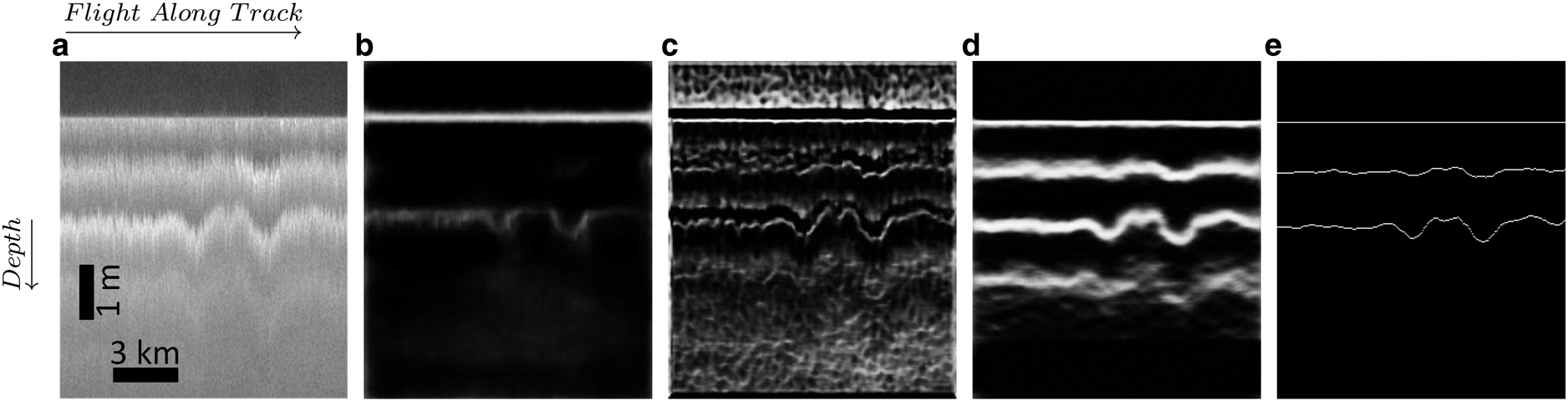
The second experiment produced a better result. We trained the model on a synthetic dataset of 1000 images (SYNT_ICE). Figure 3c shows the result of this experiment on one of the test images. The synthetic data generation process is explained in the Dataset section. As mentioned before, the simulator has not been tuned to match the actual Snow Radar data properties and statistics, but these preliminary results suggest that if we can generate synthetic data with a noise and signal generator better matched to the Snow Radar data, we may be able to achieve good results.The third experiment is conducted on our real dataset, ICE2012, with a random initialization. We notice a considerable improvement in our results. Figure 3d shows the result of this experiment on one of the test images. Figure 3e shows the annotated ground truth contours side by side of the results of our three experiments.

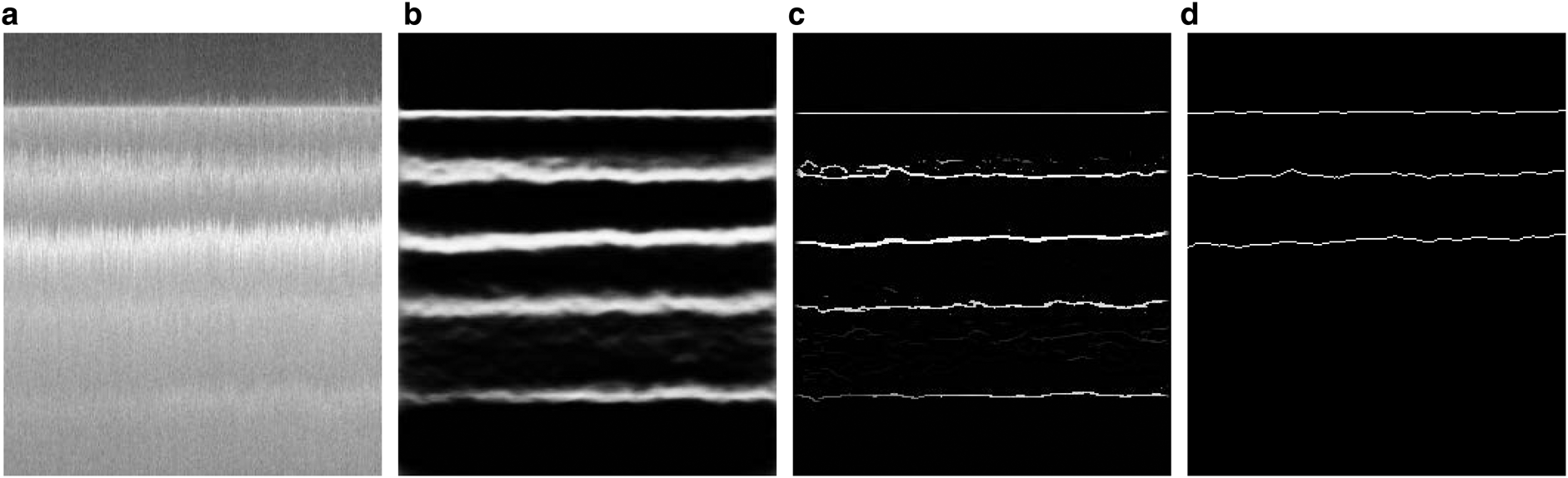
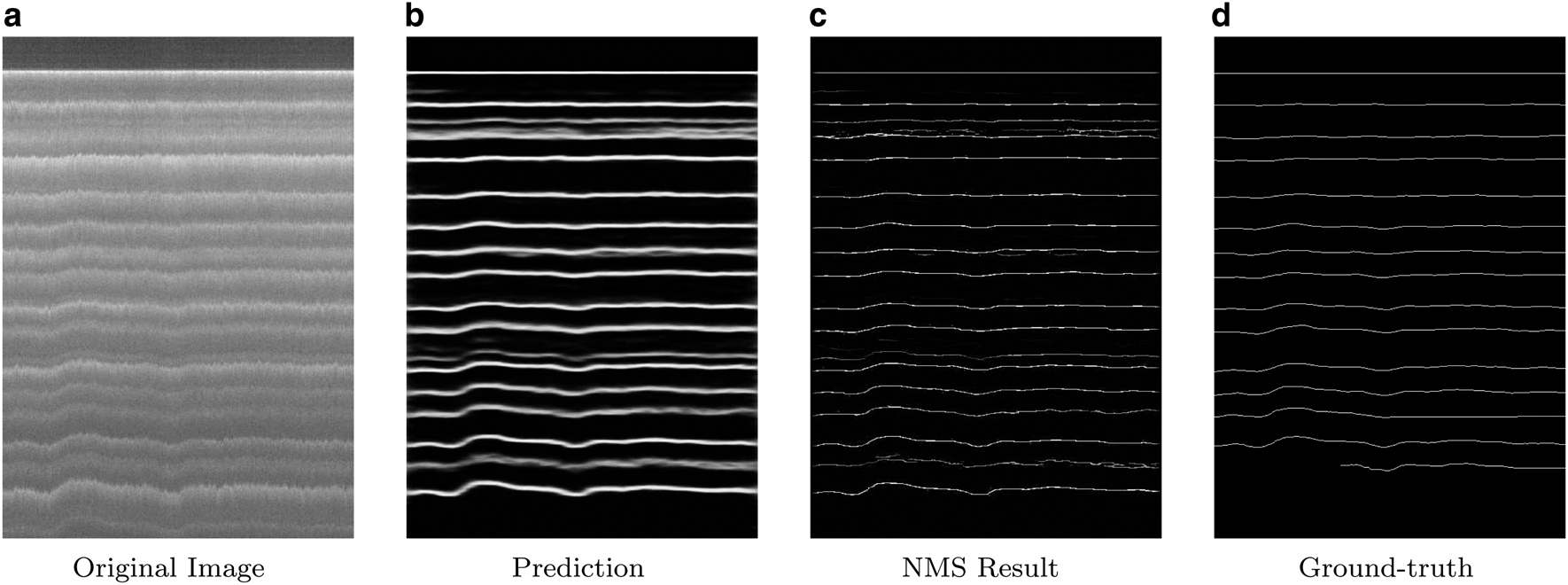
Figure 4 shows another sample of our results. In this figure, in addition to the predicted results by our network (Fig. 4b), we have also shown the post-processing results after non-maximal suppression (Fig. 4c). Non-maximal suppression (NMS) (Dollár and Zitnick, Reference Dollár and Zitnick2014) results in thinned edge maps. As we can see in Figure 4, the original image has five different layers, but only the three top layers are annotated in the ground truth image. With our training strategy, our model has been able to detect all five layers.

Fig. 4.

A test result of the ICE experiment: (a) the original image, (b) the prediction result, (c) the non-maximal suppression result, (d) the ground truth.

As it was pointed out in the previous sections, HED model produces side-outputs in different scales. Figure 5 shows all side outputs of the model and the final fusion for two images. It is apparent that the first side-outputs contain more details of the image while the later side outputs project the general structure of the image. The noise is more apparent in the first side-output while the last side-output is more enhanced.

Fig. 5.

From left to right: the first image is the first side-output which is the same size as the original image; the second image is the second side-output which is half the size of the first side-output; likewise the third side-output is half the size of the second side-output and so on. The utmost right image is the fusion of the five side-outputs.

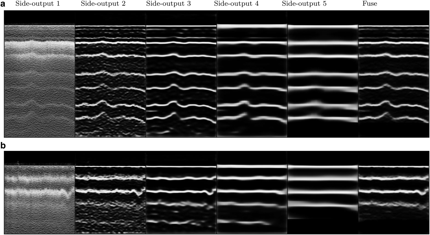
Figure 6 provides a sample result of an image with more fluctuations in the layer boundaries. Compared to the ground truth labels, our method can detect all layers including layers that are difficult to track manually.

Fig. 6.

A test result of the ICE experiment: (a) original image with sharp fluctuations in the layer boundaries, (b) the prediction result, (c) the non-maximal suppression result, (d) the ground-truth.

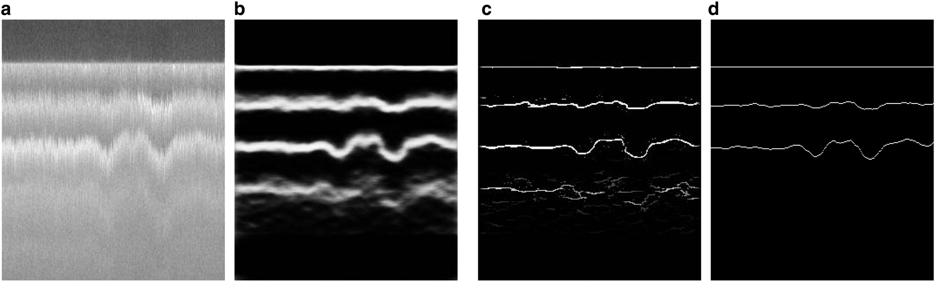
Figure 7 shows another example of how well the model works in the case of images that contain many internal layers. In this figure, the original image contains many layers. Towards the bottom of the image, the ground-truth labeled data miss tracking a couple of layers but our model (Figs b and c) is able to detect them. However, our model does fail to predict the very last bottom layer.

Fig. 7.

Another sample where the image contains a high number of layer boundaries. The model is trained and tested on ICE2012; (a) is the original image; (b) is the prediction of the deep neural network; (c) is the post-processing results after the non-maximal suppression (NMS) and finally (d) is the ground-truth result.

6.1. Quantitative results

To evaluate our results quantitatively, we have used three different metrics; The Optimal Dataset Scale (ODS) or best F-measure on the dataset for a fixed scale, the Optimal Image Scale (OIS) or aggregate F-measure on the dataset for the best scale in each image, and the Average Precision (AP) on the full recall range (equivalently, the area under the precision-recall curve) (Arbelaez and others, Reference Arbelaez, Maire, Fowlkes and Malik2011). Table 1 shows the quantitative results for all three experiments with the three aforementioned metrics (ODS, OIS, AP) for all side-outputs as well as the fuse layer. The first column in Table 1 presents the results for transfer learning in which the model is trained on the BSDS500 dataset, and tested on the real test data. The second column shows the result of the model trained on the synthetic ice data (SYNT_ICE), and tested on the real test data. The final column shows the result of training the model on real data and evaluated on the real test data. As we can see in Table 1, the third experiment (ICE) shows the most accurate results compared to the other two experiments (BSDS and SYNT). Also the fusion of all side-outputs (Fuse) presents the most accurate result compared to each individual side-output.

Table 1.

Evaluation results for the test dataset. The ICE column illustrates the result of our experiment where we trained and tested the model on the real dataset of ice images. ODS is the Optimal Dataset Scale, OIS is the Optimal Image Scale and AP is the Average Precision. This experiment provided the best results shown in bold fonts. The SYNT column: trained on the synthetic images dataset and tested on the real test data. The BSDS column: trained the model on the BSDS500 dataset and tested on the real ice images

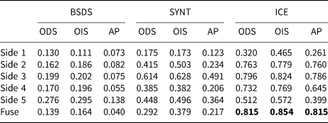
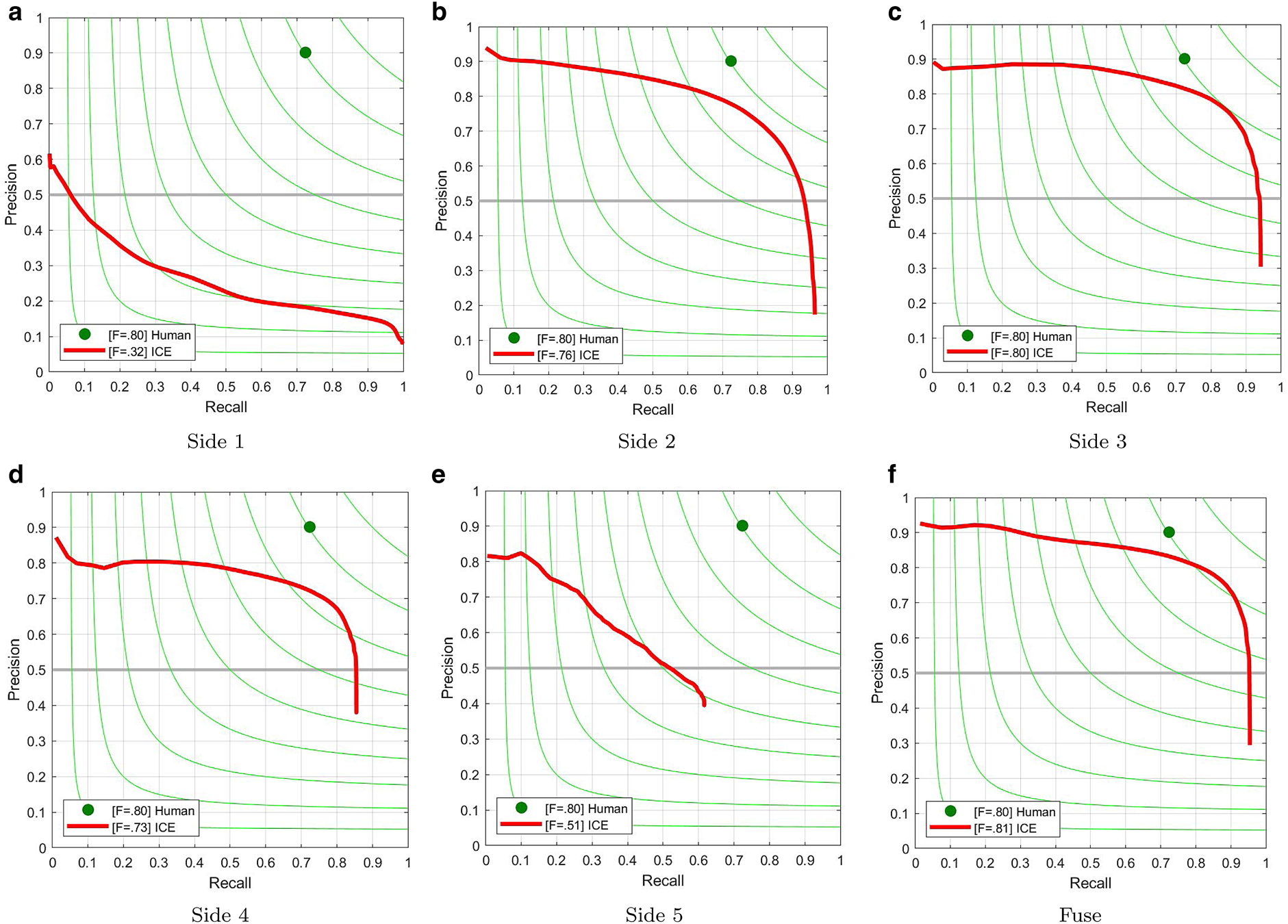
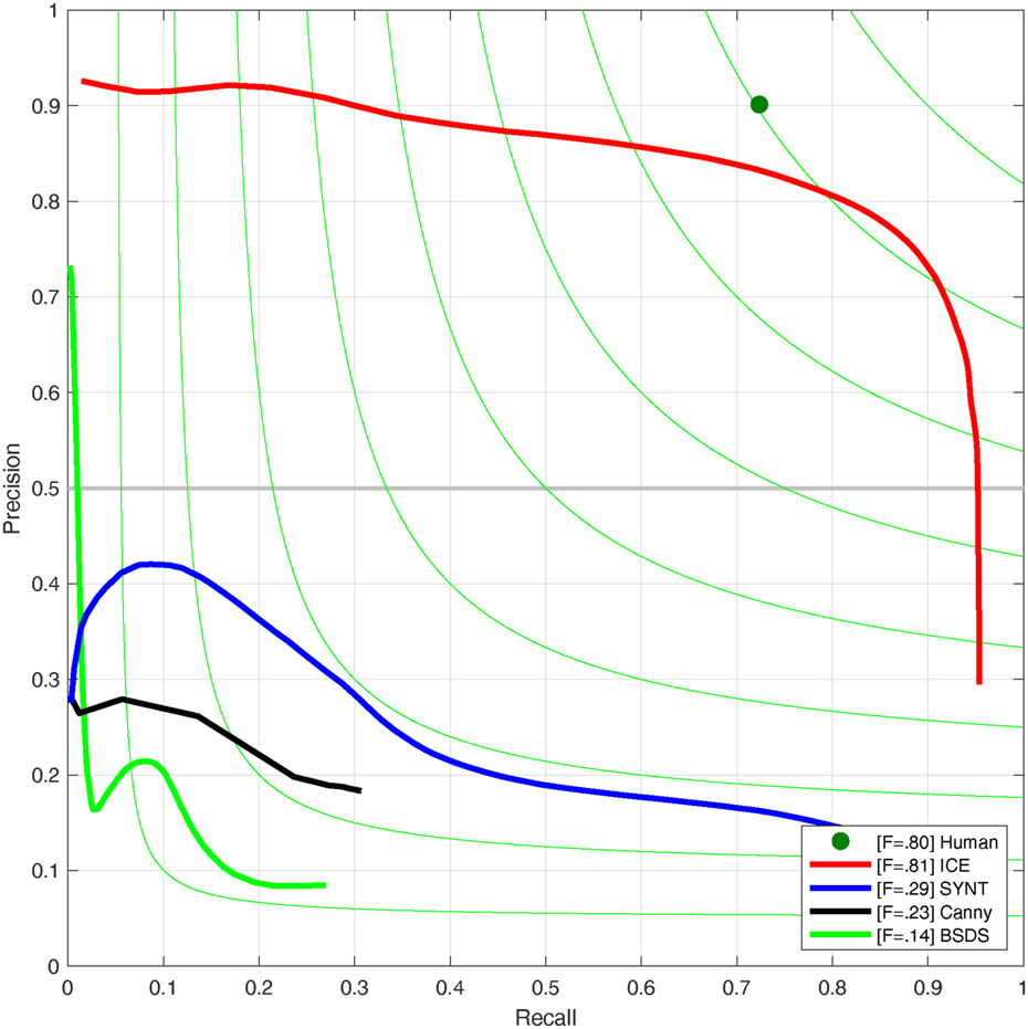
Table 2 shows the result of the three experiments in comparison to a traditional edge detection technique (Canny) using the three different metrics. We can see in this table that the deep learning results, especially the ICE experiments, show more accurate results compared to the traditional edge detection technique (Canny). We also used the precision-recall curve where the green line shows the value for F-measure. Figure 8 shows the precision-recall curve for all side-outputs for our ICE experiment. We can see in this figure that the Fuse result depicts a closer curve to the labeled data (green point).

Fig. 8.

Evaluation of the ICE experiment: precision-recall curve for each side-output and their fusion. (a) Side 1, (b) Side 2, (c) Side 3, (d) Side 4, (e) Side 5, (f) Fuse.

Table 2.

Comparison between a traditional edge detection method such as Canny, with the deep learning method trained in different ways

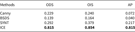
Figure 9 shows the precision-recall curve for all three experiments in addition to the traditional edge detection technique. Here also the ICE experiment presents a closer curve to the labeled data.

Fig. 9.

Evaluation comparison: precision-recall curves of various methods applied on our test set: the result of Canny edge detection method, the result of the deep learning model trained on ICE2012 dataset (ICE), BSDS500 dataset (BSDS) and Synthetic data (SYNT).