


Nomenclature
- A η
-
= control attack parameter (for control input η), per s
- A ηG
-
= guidance control attack, %
- A ηN
-
= number of control attack points, -
- A ηN-n
-
= normalised PePi control attack numbers, -
- A ηR
-
= control attack activity rate, per s
- A ηRC
-
= combined weighted adaptive control attack activity rate for all four controls, per s
- A ηR-Pr
-
= combined weighted adaptive control attack activity rate for primary control(s), per s
- A ηR-Sec
-
= combined weighted adaptive control attack activity rate for secondary control, per s
- A ηS
-
= stabilisation control attack, %
- CoF
-
= cut off frequency, Hz
- r 2
-
= coefficient of determination, -
- XA, XB, XC, XP
-
= Lateral, Longitudinal, Collective and Pedal control inputs, inch
- η
-
= pilot control deflection, inch
- ${\dot \eta _{pk}}$
-
= peak rate of control deflection, %/s

Subscripts
- i
-
= the four (XA, XB, XC and XP) controls
- Tot
-
= total number of control attack points from all four (XA, XB, XC and XP) controls
Superscripts
- avg
-
= average control attack activity rate for whole MTE
- pk
-
= peak control attack activity rate through the MTE
- loc
-
= time-varying localised control attack activity rate
1.0 Introduction
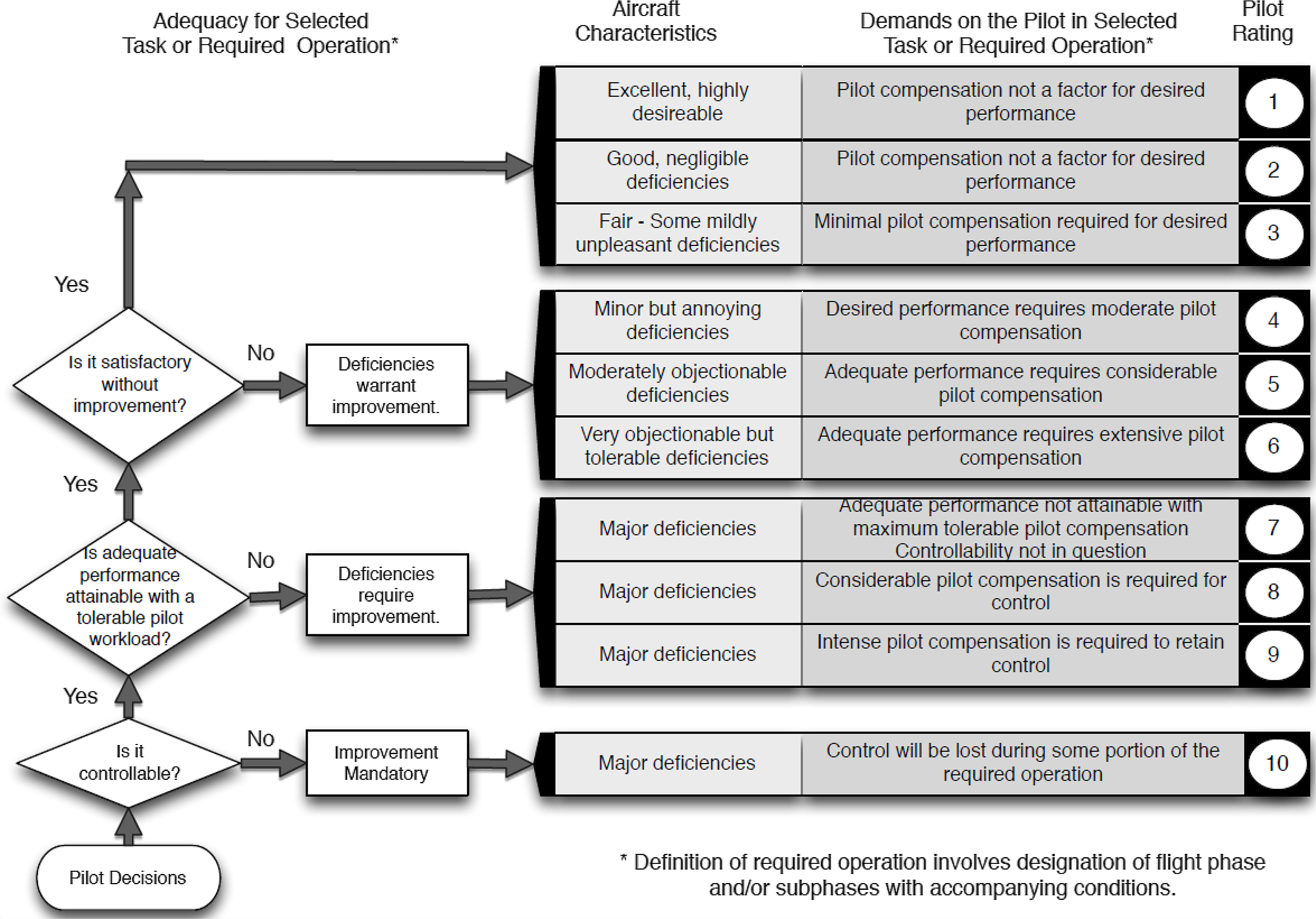
During flight and piloted simulation test campaigns, assessment of the Handling Qualities (HQs) of an aircraft is traditionally undertaken with Test Pilots (TPs) awarding Handling Qualities Ratings (HQRs) using the scale developed by Cooper and Harper in 1969 [Reference Cooper and Harper1]. While the scale was developed for the evaluation of an aircraft’s HQs, it has also been used in the assessment of flight simulation fidelity by comparing HQRs in flight and simulation [Reference Perfect, Gubbels, White, Padfield and Gubbels2–Reference Hess and Malsbury4]. The HQR became a critical component of the US Army’s handling qualities standard, ADS-33E-PRF [5]; the subjective element for the assigned HQs of the HQ assessment process. A fundamental element of the HQR process is to report the control compensation required to overcome any vehicle system deficiencies that could inhibit the pilot from flying a task to operationally relevant performance and safety standards. According to Cooper and Harper [Reference Cooper and Harper1]:
“Pilot compensation as used in the scale is intended to indicate that the pilot must increase his workload to improve aircraft performance. It relates to the pilot’s difficulty in completing a task with the precision required for that task.”
Cooper and Harper defined pilot compensation as [Reference Cooper and Harper1]:
“The measure of additional pilot effort and attention required to maintain a given level of performance in the face of less favourable or deficient vehicle characteristics”
Moreover, Cooper and Harper defined the total pilot workload as [Reference Cooper and Harper1]:
“The workload due to compensation for aircraft deficiencies plus the workload due to the task”
It should be noted that, although the pilot’s workload is reflected in the HQR, the HQR is not strictly a measure of the workload but rather reflects the control compensation element i.e. the additional effort above the task workload to achieve a given level of performance. Understanding that there is always a workload due to the task, that is separate from compensation, is fundamental to awarding an HQR.
The HQR scale incorporates a decision tree structure (Fig. 1), which ensures that the HQR couples:
-
(a) the extent of the HQ deficiencies (no worse than mildly unpleasant (Level 1), minor to very objectionable (Level 2), major (Level 3) or so severe that there is a high risk of loss of control (HQR 10)),
-
(b) with the achieved performance (desired, adequate, inadequate),
-
(c) and the required compensation (not a factor, minimal, moderate, considerable, extensive, maximum tolerable, controllability in question) [Reference Cooper and Harper1].
Cooper-Harper Handling Qualities Rating Scale [Reference Cooper and Harper1].
When an HQR is awarded, it is important that the reason(s) for the rating is (are) made clear. There may be several causal factors and consequent impacts, and they should all be described by the TPs as part of the assessment.
Although the HQRs, along with the achieved performance and the compensation descriptors, provide insight into the consequences of HQ deficiencies of the vehicle system, the ratings will be ‘affected’ by individual pilot biases, the subjective element of making the award [Reference Paul and Rhinehart6]. This includes inter- and intra-pilot variability, training and operational background, situational awareness, fatigue level and environmental factors. The HQR is absolute, not relative, and the scale is a non-linear function of its component influences [Reference Wilson and Riley7, Reference Harper and Cooper8]. There have been concerns regarding how HQRs are awarded by a pilot for tasks [Reference Paul and Rhinehart6] such as the ADS-33 Mission Task Elements (MTEs) [5]. For example, it might be that for 75% of the MTE, the desired performance is achieved, while for some element of the MTE the pilot is challenged to achieve adequate performance. A debate has been to understand whether the HQR is, or should be, awarded for a particularly difficult local phase within the MTE or is an average of compensation/performance achieved throughout the MTE. The ADS-33 Test Guide [Reference Blanken, Hoh, Mitchell and Key9] is unclear on this point, but the assessment methodology does require three TPs to fly the MTEs, and the average of their ratings is used to determine the qualification outcome. A recent study reported in Ref. (Reference Paul and Rhinehart6) examined this issue based on a discussion with staff from the US Naval Test Pilot School (USNTPS) and revealed that “the pilots are not explicitly instructed to consider the peak or average workload over the total task, leaving an open question which could contribute to both inter- and intra-pilot variability” [Reference Paul and Rhinehart6]. In support of the research presented in the present paper, discussions were carried out on the topic of pilot compensation and adaptation with a range of TPs active in the Liverpool’s research. One of the key discussion topics was to understand whether the HQR awarded is averaged across an MTE or is based on the phase of the MTE where the worst deficiencies were experienced (i.e. a peak factor). There was agreement amongst the TPs for the peak-factor approach, since the averaged HQR could disguise a potential operational limitation or task phase where risks to safety and performance would be increased.
With the variable influences on subjective assessment, coupled with a desire to better understand the pilot-vehicle system interactions, the development of a robust metric for the quantification of the pilot control compensation has been a subject of interest for the HQ community for many years [Reference Perfect, Gubbels, White, Padfield and Gubbels2, Reference Paul and Rhinehart6, Reference Lampton and Klyde10–Reference Jennings, Craig, Carignan, Ellis and Thorndycraft13]. To this end, several studies have been conducted on the development and use of control compensation metrics and methodologies. These include, Time-Domain (TD), Frequency-Domain (FD) and combined Time-Frequency Domain (TFD) measures based on the pilot control activity and aircraft states [Reference Perfect, Gubbels, White, Padfield and Gubbels2, Reference Paul and Rhinehart6, Reference Lampton and Klyde10–Reference Tritschler, O’Connor, Holder, Klyde and Lampton12], and the psychophysiological and neurological measures based on the assessment of the encephalography and heart-rate signals, and the eye and head movements [Reference Law, Jennings and Ellis14–Reference Hankins and Wilson16]. The utility of these metrics has been demonstrated in different applications; however, the research presented in the present paper is focused on the measures based on the pilot control activity which are reviewed and discussed in greater detail in the following section. The main aim behind developing such a metric is that it can support the HQ analysis along with the assessment of the piloting styles and strategies that will help understand the reasons behind any spread of HQRs across the pilots. Moreover, in terms of its applications, the metric can support pilot training needs, design, development and qualification of flight control systems, accident investigations, certification of rotorcraft and simulators, and simulator fidelity assessment [Reference Perfect, Gubbels, White, Padfield and Gubbels2, Reference Paul and Rhinehart6]. However, a standardised compensation metric that fulfils the needs of these applications has remained a challenge and is a goal in the Liverpool research.
This paper reports progress on the development of such a Control Compensation Metric (CCM). The new weighted-adaptive metric is used to correlate subjective pilot assessments with pilot control activity. Moreover, in combination with a time-varying FD technique, the proposed metric can aid the understanding of the overall subjective assessments. Finally, by combining the subjective and proposed CCM, compensation boundaries can be derived by combining results from a range of MTEs. The CCM is intended to be complementary to the HQR, informing the HQ-deficiency analysis. Different applications envisaged might be situations where HQRs are not given, e.g. analysis of training exercises, analysis of accident data and control-workload assessment in trials involving pilots unfamiliar with the HQ process.
The paper is organised as follows: Section 2 reviews the literature on objective pilot control compensation measures. Section 3 provides details of the facilities used in the tests reported in the paper, the predicted HQs and the techniques used in assessing candidate metrics in the pursuit of a CCM. Section 4 shows the application of the proposed CCM for two case studies involving five different MTEs flown in flight and in a simulator using two aircraft configurations. Section 5 presents the proposed objective-subjective compensation boundaries derived using the CCM metric. Section 6 summarises the overall procedure of the CCM application as a guideline for pilot compensation assessment. Conclusions and future work are presented in Section 7.
2.0 Objective compensation measures: Background
In the field of HQ engineering, several pilot compensation/workload metrics have been explored using a range of different analytical approaches.
Padfield et al. formulated the control attack metric, A η , based on the rate and magnitude of the pilot’s control input [Reference Padfield, Jones, Charlton, Howell and Bradley17], along the lines of the attitude quickness parameter to quantify agility [5]. The control attack concept was utilised in Liverpool’s Lifting Standards (LS) project: “A Novel Approach to the Development of Fidelity Criteria for Rotorcraft Flight Simulators”, as part of a set of metrics (Attack Activity Rate, Mean Peak Control Rate, Mean Control Displacement) to reflect pilot control compensation [Reference Perfect, Gubbels, White, Padfield and Gubbels2]. The metrics were used to assess the differences between flight and simulation tests performed by a single TP on a range of ADS-33 MTEs. The control attack metric has been extended in the present research and is discussed in greater detail in Section 3.
Bachelder and Aponso introduced a spare mental-capacity estimator, the “Bedford Estimator”, based on the pilot stick position and display error [Reference Bachelder and Aponso18]. The Bedford Estimator was later renamed the “Spare Capacity OPerations Estimator (SCOPE)” [Reference Bachelder19]. Comparisons between the SCOPE metric and the Bedford Pilot Workload Ratings (BWRs) were examined for a tracking task that provided a high correlation coefficient of 0.93. More recently, Bachelder et al., have extended SCOPE to assess the HQRs for the Slalom MTE using a workload and parameter estimation methodology which examines the HQR scale from an integrative perspective of performance and pilot compensation [Reference Bachelder, Lusardi, Aponso and Godfroy-Cooper11]. The assessment demonstrated a good correlation between the pilot’s assigned and SCOPE-estimated HQRs over varying aircraft and inceptor system dynamics [Reference Bachelder, Lusardi, Aponso and Godfroy-Cooper11].
Recently, Paul and Rhinehart conducted a study in which various inceptor activity measurements, such as power frequency, peak inceptor rate, aggressiveness metric and duty cycle, were investigated, along with the introduction of a new concept of quantifying the interaction of control contributions in a multi-axis task, the orthogonality metric [Reference Paul and Rhinehart6]. The study examined the utility of the metrics’ correlation with reported HQRs for a simulated approach and hover task of a representative H-60 helicopter model operating to a DDG-class ship using the USNTPS’ fixed-base simulator. By examining the linear fit for a range of different pilots, the study concluded that, due to differences in individual pilots’ styles, it was not possible to obtain a universal inceptor workload metric that correlated across pilots and, thus, some individual pilot baselining may be required for practical application of the metrics. The authors suggested that the correlation could be improved by using a more appropriate correlate and/or a more clearly designed task [Reference Paul and Rhinehart6].
Blanken and Pausder introduced a frequency domain measure of pilot control activity, the Cut-off Frequency (CoF) metric [Reference Blanken and Pausder20], derived from the power spectral density of the pilot control signal [Reference Blanken and Pausder20, Reference Tischler and Remple21]. The CoF measure was also used in the LS research along with the control attack metrics [Reference Perfect, Gubbels, White, Padfield and Gubbels2]. While CoF has been shown to be useful in a variety of applications [Reference Atencio3, Reference Fujizawa, Lusardi, Tischler, Braddom and Jeram22], recent studies have compared the CoF with BWRs and HQRs, which have shown no distinct correlation [Reference Lampton and Klyde10, Reference Bachelder and Aponso18]. In the present research, the utility of the CoF metric has been assessed along with the attack metric in Section 3.
Jones et al. demonstrated a wavelet analysis technique for the decomposition of the pilot control activity into discrete components, so-called worklets, that can be associated with Guidance and Stabilisation (G&S) components in a task and identified the two distinct workload components [Reference Jones, Padfield and Charlton23]. The decomposition of the pilot control into G&S activity helps in the identification of the changes in the pilot control activity associated with varying task difficulty or HQ deficiencies. Previous studies have discussed the relationship of these two components within two different frequency bands of control activity; one associated with the flight-path geometry (sometimes referred to as the task-bandwidth, associated with guidance: typically <0.5Hz) and the other with the aircraft attitude (associated with stabilisation: typically 1–2.5Hz) [Reference Padfield, Jones, Charlton, Howell and Bradley17, Reference Jones, Padfield and Charlton23]. By comparing the frequency content of the pilot control activity within two different frequency bands, the different components of pilot workload can be quantified. However, it should be noted that the two are by no means independent; stabilisation is likely to be superimposed on guidance when the latter requires strong control [Reference Jones, Padfield and Charlton23]. In Ref. (Reference Padfield, Jones, Charlton, Howell and Bradley17), the authors make the point that this mixing of task workload and the required compensation depends critically on the ratio of task bandwidth to aircraft attitude bandwidth, effectively the number of attitude changes required in the task time. In the present study, a new complementary concept for the G&S control activity assessment is introduced based on the control attack concept.
Lampton and Klyde used a wavelet transform-based TFD metric, called the scalogram, to characterise rotorcraft-pilot-vehicle system interactions and to calculate time-varying CoF throughout a manoeuvre [Reference Lampton and Klyde10]. Scalograms represent the spectrum of frequencies within the control input as a function of time. Later, the metric was successfully used to detect pilot induced oscillations within the flight and simulation test databases [Reference Klyde, Schulze, de Mello and Mitchell24, Reference Cameron, Cunliffe, White, Klyde and de Mello25]. Moreover, Tritschler et al. described the use of TFD methods to analyse the pilot control activity for an OH-58C Kiowa helicopter performing the pirouette MTE [Reference Tritschler, O’Connor, Holder, Klyde and Lampton12]. The study concluded that these post-flight analysis methods were best suited for inter- and intra-pilot comparisons providing additional information or insight when pilot ratings and comments are available. In the present study, a TFD metric has been extended in conjunction with the attack and CoF metrics.
Despite significant research in developing quantitative compensation metrics, there remains a need for an objective metric that correlates across TPs, having different piloting styles and employing different control strategies, and a wide variety of MTEs having different dominant control axes and performance requirements. Previous research has primarily focused upon examining the utility of different metrics for a single MTE or by considering controls in a separate non-combined format (i.e. independent of other control axes). This paper focuses on the development of a multi-axis adaptive pilot CCM that can be used in the HQ assessment process for a range of MTEs.
3.0 Research methodology
This research has used some of the flight and simulator test data gathered in the LS project [Reference Perfect, Gubbels, White, Padfield and Gubbels2]. As part of this work, a series of flight and simulator experiments were conducted using the National Research Council (NRC) Canada’s Bell 412 Advanced Systems Research Aircraft (ASRA) [Reference Gubbels and Ellis26] and Liverpool’s HELIFLIGHT-R simulator [Reference White, Perfect, Padfield, Gubbels and Berryman27], using ADS-33 MTEs. Within the test campaigns, two aircraft configurations, a Bare Airframe (BA) configuration i.e. with no flight control augmentation, and an augmented configuration featuring an Attitude Command/Attitude Hold (ACAH) response type, were flown by two test pilots. The MTEs included hover/low-speed tasks (Precision Hover (PH), Pirouette, (Pr) and Lateral Reposition (LR)), and forward flight tasks (Roll Step (RS), Acceleration-Deceleration (AD)) [5, Reference Meyer and Padfield28]. The MTE descriptions are provided in Appendix A.
3.1 Research facilities
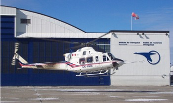
3.1.1 NRC Bell 412 Advanced Systems Research Aircraft (ASRA)
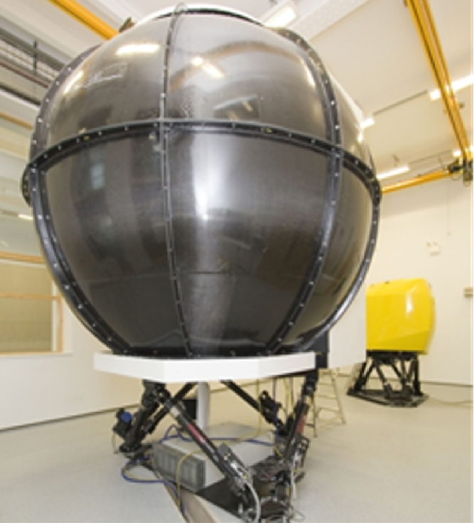
The Bell 412 ASRA (Fig. 2) complements the experimental work carried out in the HELIFLIGHT-R simulator through its key capability, the full authority experimental Fly By Wire (FBW) flight control system, allowing the aircraft to be operated as an in-flight simulator [Reference Gubbels and Ellis26]. ASRA’s flight data recording system consists of a range of data monitoring and measurement equipment, facilitating the assessment of the pilot control activity and aircraft task performance analysis. The FBW system enables the implementation and testing of new control laws in flight.
NRC ASRA Bell-412 Aircraft [Reference Perfect, Gubbels, White, Padfield and Gubbels2].

3.1.2 HELIFLIGHT-R simulator
The University of Liverpool’s Flight Science and Technology research group operates a fully reconfigurable research simulator, HELIFLIGHT-R (Fig. 3); acceptance and commissioning of the simulator was completed in 2008 [Reference White, Perfect, Padfield, Gubbels and Berryman27]. The simulator has a three-channel 230° × 70° Field of View computer image generation system, a 6-degree-of-freedom hexapod motion platform, a four-axis force-feedback control loading system and an interchangeable crew station. Flight dynamic models are developed in either FLIGHTLAB [Reference Du Val and He29] or MATLAB®/SIMULINK® and the current aircraft library features a range of fixed-wing, rotary-wing and tilt-rotor aircraft. The outside world environment is generated using the Presagis Creator Pro software, which is integrated with Presagis’ VEGA software into the Liverpool Virtual Environment. The visual and motion cues, together with sound cues, provide a powerful immersive simulation environment for a pilot [Reference White, Perfect, Padfield, Gubbels and Berryman27].
HELIFLIGHT-R Simulator (foreground) [Reference White, Perfect, Padfield, Gubbels and Berryman27].
3.2 Predicted Handling Qualities
Handling Qualities engineering features two major dimensions – the predicted HQs and the (pilot) assigned HQs [Reference Padfield30]. In a formal application of ADS-33, in an acquisition process both must meet Level 1 standards. In a research application, any analysis of HQRs and pilot control compensation needs to be informed by the associated predicted HQs to aid understanding. The ADS-33 Hover and Low-Speed HQ predictions for the ACAH and BA configuration of the ASRA and the FLIGHTLAB simulation model, the F-B412, are summarised in Table 1. The table specifies the HQ levels 1, 2 and 3 with green, yellow and red colouring, respectively for the All-Other-MTEs category.
Summary of Predicted HQs of ASRA aircraft and simulator model for hover and low speed (green – Level 1, yellow – Level 2, red – Level 3)
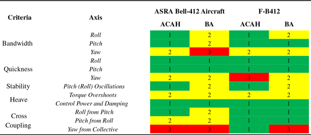
The RS and AD MTEs will be impacted by additional forward flight HQs, but these align fairly closely with the results in Table 1. Generally, the ACAH configuration is Level 1 and the BA configuration Level 2. Exceptions can be seen for ACAH yaw quickness, BA bandwidth and some cross-coupled responses. In terms of the HQ expectations for different MTEs, the PH and Pr are generally low to moderate aggression tasks that require small-amplitude corrective inputs. For the PH, the bandwidth will be the dominant concern, along with cross couplings, in the stabilisation phase. For the Pr MTE, roll/pitch attitudes are expected to remain below 10/5°, and perturbations from the steady turn rate should be small. However, the degraded yaw bandwidth is likely to feature in this regard. The ASRA cross-couplings are mostly Level 2 and 3 except for Level 1 roll/pitch for the ACAH configuration. For the F-B412, the cross-couplings are Level 1, except for Level 3 yaw/collective for the BA configuration. The AD and LR MTEs, in contrast, are moderate to high aggression tasks that require medium to large attitude changes. While bandwidth and cross-couplings play an important role in the tasks, in the hover capture and stabilisation phases, deficiencies in attitude quickness can also contribute to pilot compensation. The primary response parameters (bandwidth and quickness) in pitch and roll are predicted as Level 1–2, and the yaw axis as Level 2–3, which will demand additional compensation from the pilot in maintaining a constant heading. Furthermore, it would be anticipated that in flight, the Level 2–3 coupling effects (especially roll/pitch/roll and collective-yaw for the AD; and pitch/roll for the LR) are likely to impact the achieved precision and increase the compensation compared with the simulator.
Overall, we expect pilots awarding Level 1–2 HQRs when flying the ACAH configuration in MTEs that do not have significant yaw and collective requirements. The extent of the Level 2 and 3 HQs for the ASRA BA configuration may push HQRs into Level 3.
3.3 Objective compensation metrics development
This section presents the development process undertaken in the pursuit of a CCM, which includes the assessment of several candidate metrics leading to the development of an adaptive-weighted metric.
3.3.1 Control attack
In the LS research, measures of the pilot control activity were used in attempts to quantify the pilot control workload [Reference Perfect, Gubbels, White, Padfield and Gubbels2]. One of the measures used was the control attack parameter, A
η
(Equation (1)), introduced earlier. The A
η
characterises each discrete control input and is defined as the ratio of the peak rate of control displacement, ${\dot \eta _{pk}}$
, to the magnitude of the change in the control displacement, Δη.
${\dot \eta _{pk}}$
, to the magnitude of the change in the control displacement, Δη.
 \begin{align}{A_\eta } = \frac{{{{\dot \eta }_{pk}}}}{{\Delta \eta }}\end{align}
In broad terms, higher attack values indicate rapid-small control deflections while a lower attack value indicates slower-large control deflections. As with the ADS-33 attitude quickness parameter [5], the attack approximates the inverse of the time to change for a simple ramp. An example of a high attack and low attack pilot control input are shown in Fig. 4.
Control deflection (lateral cyclic) time history showing high (Aη2) and low (Aη1) values of attack.

The origin of the attack metric in control analysis goes back to Ref. (Reference Padfield, Jones, Charlton, Howell and Bradley17), and relates to the property of a sound envelope in music, where the attack is the time taken for the initial run-up of level from nil to peak, so strictly the inverse of how it is used in control activity analysis. Figure 5 shows an example of two ideal control inputs; decisive and quick, and smooth and slow, having ramps of different slopes.
Ideal control inputs showing two ramps of different slopes; decisive and quick, smooth and slow.

The Attack Number (A ηN ) and Attack Activity Rate (A ηR ) metrics are defined as:
-
(a) Attack Number (A ηN ): the total number of times that the pilot displaces a particular control having a magnitude higher than a specified threshold value. Discussion on the appropriate value of the attack thresholds comes later in this section.
-
(b) Attack Activity Rate (A ηR ): the ratio of the total number of A η to the time length of the MTE. It can be defined as the ‘busyness’ metric and an average for an MTE.
3.3.1.1 Control attack threshold
When assessing different attack-based metrics to examine correlations with HQRs awarded by a pilot, it is important to determine a threshold value for what might be described as a productive pilot control input. To explore this approach, the threshold was increased in equal intervals and the impact on the A ηN and A ηR registered within different MTE phases was examined.
Figure 6 presents an example of a RS MTE performed in the simulator (see Appendix A: Table A5). Figure 6(a) and (b) show the aircraft’s ground track and the pilot lateral cyclic control activity XA, respectively. The gates (G) for the RS MTE are specified as numbered stars in Fig. 6(a). Figure 6(c) and (d) show the XA control attack for the whole MTE (combined) and spatially segmented-MTE, respectively. Results for two attack thresholds (0.25 and 2.5%) are compared. The control position threshold percentage is calculated for the full control travel range, −50% to +50% (i.e. −6.14:6.33in for XA; −6.1:6.1in for XB; 0:10.7in for XC; −3.92:2.86in for XP).
Control attack threshold selection and segmentation approach, (a) Aircraft track; (b) Lateral pilot stick input; (c) Combined control attack; (d) Segmented control attack.

Using the 0.25% threshold, Fig. 6(c) shows a significant number of the low amplitude-high attack values captured. To spatially identify whether the control activity associated with these attack points was deliberate and required or not, the MTE is divided into segments, enabling examination of pilot compensation in different MTE phases. In this case, five segments were examined based on the positioning of the gates used to traverse the runway (i.e. G4–G6 for the Left Hand Side (LHS) to Right Hand Side (RHS) runway crossing and G9-G13 for the RHS to LHS runway crossing), as shown by the vertical dashed lines in Fig. 6(a) and (b), respectively.
Figure 6(d) shows five subplots associated with these segments. The 1st segment (Start-G4) represents the run-up to the beginning of the MTE (i.e. between −1,000 to 1,500ft runway track) and was used to define the threshold. In this segment, there are no specific task requirements and thus the pilot should not have to apply G&S control inputs, as the simulation model is trimmed, until just before the end of the segment to initiate the turn at G4. Any attack points registered before the turn are considered unproductive from the task perspective, as they do not contribute to G&S elements required along the runway edge. However, this segment does show a relatively large number of low-amplitude high-attack points from Fig. 6(c). The threshold was increased in equal intervals of 0.25% until a single deliberate guidance control attack featured in the first segment, required to initiate the turn. This was achieved at the threshold of 2.5%, as shown in Fig. 6(d)-1st (Start-G4) segment as a star marker. It should be noted that for all the following attack analysis, the threshold of 2.5% is used.
Table 2 shows A ηN and A ηR metrics for the segmented attack charts shown in Fig. 6(d), respectively, for 0.25 and 2.5% threshold and their percentage difference. It can be seen that, in the first segment, nearly 90% of the attacks have been filtered out using a 2.5% threshold. To gain more insight and confidence in the suitability of the new attack threshold, a moving window-based time-localised attack metric was formulated for comparison with the TFD metric.
Segmented control attack metric calculated using 0.25 and 2.5% threshold for the data presented in Fig. 6(d)

3.3.1.2 Time-varying localised attack activity rate
How the attack parameter is used to correlate with the HQR connects with the idea of a peak or an average rating across the MTE. Using the average A ηR for the whole MTE can mask local peaks, making it difficult to identify the phase(s) within the MTE where a pilot might be struggling with HQ deficiencies of the vehicle. This section presents a time-varying attack activity rate metric A ηR loc , formulated to capture local control peaks in an MTE that would help in identifying where the pilot is working the hardest, and the dominant area of compensation. The method includes the formulation of a control segmentation approach using a moving 5s window, with 2.5s overlap. The 5s window is selected based on the minimum time needed for the pilot to perceive visual cues and successfully execute a manoeuvre within an MTE [Reference Padfield, Clark and Taghizad31].
Figure 7 shows an example of the XA A ηR loc metric along with the aircraft runway track and pilot control input compared for the two simulated aircraft model configurations flown in the RS MTE [Reference Cameron, Memon, White and Padfield32]. Config A represents a baseline simulation model of the ASRA, whilst Config B represents an improved fidelity simulation model developed to better match flight test data [Reference Cameron, Memon, White and Padfield32]. Figure 7 shows differences in the A ηR loc during different phases through the MTE. As the pilot enters the first LHS-RHS crossing (t = 17.5–27.5s), the A ηR loc increases to >1/s in both cases. The phase (t = 30–37.5s) corresponds to the tracking phase on the RHS edge of the runway. Here, the A ηR loc for Config B increases to 1.4/s, the pilot sustaining this level through to the final tracking on the LHS of the runway, where the A ηR loc reduces to about 0.5/s. For Config A, the A ηR loc reduces to 0.2/s during the RHS runway tracking, but then builds up to a high attack level of 1.8/s during the final LHS tracking; the pilot struggling to maintain track during this, largely, stabilisation phase. Reference (Reference Cameron, Memon, White and Padfield32) discusses the impact of the natural frequency and relative damping of the lateral-directional oscillation on the required compensation, explaining the difference between configurations A and B in terms of these dynamic stability characteristics.
Time-varying localised AηR loc (star markers define RS MTE phases).

With such large variations in the A ηR through the MTE, using the average attack can be misleading in terms of the HQR assigned and will not help in the identification of the dominant compensation phase(s).
3.3.1.3 Time-frequency domain and attack-rate metric composite
In the TFD, Fourier transform-based spectrograms [Reference Tritschler, O’Connor, Holder, Klyde and Lampton12] have been used to examine the characteristics of the pilot control inputs, complementary with the A ηR control metric. A spectrogram is a three-dimensional visual representation of the spectrum of frequencies within the control input as a function of time. It defines the signal in terms of time, frequency and magnitude.
In this paper, composite TFD-A ηR loc charts have been developed to demonstrate the applicability of the A ηR metric in assessing pilot control compensation. Figure 8 shows another example for the RS MTE. The central spectrogram contour-plot (formulated using a moving 4s window; selected to provide a suitable resolution in both time and frequency, thus highlighting key features of the control signal) shows the time and frequency on the abscissa and ordinate, respectively, with the colour bar indicating the magnitude of the Short-Time Fourier Transform (STFT) of the control signal; the outer plots show the time history (upper), Fast Fourier Transform (FFT, left) and A ηR loc (lower).
Composite TFD-AηR metric plots for lateral cyclic control activity [Reference Cameron, Memon, White and Padfield32].

Using this presentation form, details in different phases of the MTE can be observed, along with information for the frequency content as a function of time. The FFT shows the dominant peak around 0.15Hz (0.94rad/s), corresponding to the large control movements during the runway crossing, with a duration of about 10s at 90kn. The spectrogram and A ηR loc variations show where in the MTE the pilot is working the hardest. The two obvious peaks (@ 27.5 and 45s) are at the runway crossings, and particularly re-establishing track over the runway edges. The A ηR loc , in combination with the TFD, provides complementary insight into the compensation required to complete the task.
3.3.1.4 Combined multi-axis attack activity rate metric
So far, the attack metrics have been utilised in single-axis form and do not capture multi-axis control compensation in a complex MTE. A method for calculating a combined attack metric, including all four controls, is required. Moreover, due to the variations in piloting strategy and different levels of control compensation applied by different pilots, it is important that the accumulation methodology is adaptive to these variations.
To address this, a weighted-adaptive formulation has been developed that weights individual control A ηR contributions with the corresponding fraction of the total control attacks (A ηNTot ) applied in that axis (Equation (2)).
 $$\matrix{{{{{A_{\eta Ni}}} \over {{A_{\eta NTot}}}}} \hfill \cr}$$
where i corresponds to the four (XA, XB, XC and XP) controls.
This is calculated for each control (XA, XB, XC and XP) and then summed to obtain a combined, weighted adaptive metric A ηRC (Equation (3)).
 $$\matrix{{{A_{\eta RC}} = {{\sum\nolimits_{i = XA}^{XP} A }_{nRi}}.{{{A_{\eta Ni}}} \over {{A_{\eta NTot}}}}} \hfill\cr} $$
Alongside the A ηRC , the combined A ηR for the primary A ηR-Pr and secondary A ηR-Sec controls separately have been computed in the MTE investigations. To calculate these, the same formulation as defined in (Equation (2)) has been used by accumulating the specific controls only. The primary and secondary controls are different for each ADS-33 MTE based on the task performance requirements, see Table 3. The concept of the primary and secondary controls is discussed in the following section.
Primary and secondary controls for ADS-33 MTEs

The application of the combined adaptive A ηRC metric will be demonstrated in Section 4, by examining the correlation with the HQRs awarded by the pilots for a range of MTEs with different task performance requirements and dominant control axes. But first, we return to the separation of control functions as G&S.
3.3.2 Guidance and stabilisation control
Another key interest in the study of pilot control compensation is to identify the regions of G&S components [Reference Jones, Padfield and Charlton23]. To explore this using the attack metric, a new approach based on the concept of the Perfect Pilot (PePi) strategy is introduced in this study.
PePi is defined as the pilot who does not need to apply any compensation to fly an MTE, and so all the control movements (primary and secondary) contribute directly to the task performance. The PePi is based on the guidance control activity only and the guidance frequency for an MTE is approximated as the inverse of the time for the required flight-path change. Another way of looking at this is that the stabilisation activity is only ever required to suppress external disturbances, errors of judgement or natural mode transients, so should be minimal for the types of MTE examined in this paper.
Consider the example of the RS MTE, flown at 90kn, shown in Fig. 9, in which the primary MTE state and flight-path change are the roll attitude and lateral position, and the primary control is XA. Focussing on the first runway crossing, to complete this phase, there are three primary roll attitude changes required; the first to initiate the crossing ( $ \delta\phi \approx +30^{\circ}$
), second for the roll-reversal (
$ \delta\phi \approx +30^{\circ}$
), second for the roll-reversal ( $ \delta\phi \approx -50^{\circ}$
) and third for lining up with RHS runway edge (
$ \delta\phi \approx -50^{\circ}$
) and third for lining up with RHS runway edge ( $ \delta\phi \approx +20^{\circ}$
). This assumes that the pilot does not level off after the first turn and fly straight for a period during the crossing. Each roll attitude change is achieved with a certain quickness; the ratio of the peak attitude rate to the attitude change [Reference Padfield, Jones, Charlton, Howell and Bradley17], and each roll quickness is achieved by the pilot applying primary XA input. With a Rate Command (RC) response type, two stick movements (i.e. a pulse) are required. Whereas, for an ACAH response type, a single stick movement (i.e. a step or more realistically a ramp) is required. Associated with each stick movement, there is an attack parameter. For the RC aircraft, there are six XA attacks and three for the ACAH, during crossing.
$ \delta\phi \approx +20^{\circ}$
). This assumes that the pilot does not level off after the first turn and fly straight for a period during the crossing. Each roll attitude change is achieved with a certain quickness; the ratio of the peak attitude rate to the attitude change [Reference Padfield, Jones, Charlton, Howell and Bradley17], and each roll quickness is achieved by the pilot applying primary XA input. With a Rate Command (RC) response type, two stick movements (i.e. a pulse) are required. Whereas, for an ACAH response type, a single stick movement (i.e. a step or more realistically a ramp) is required. Associated with each stick movement, there is an attack parameter. For the RC aircraft, there are six XA attacks and three for the ACAH, during crossing.
The RS requires the pilot to maintain height and speed within defined margins and pass through the gates within margins on lateral position and heading. The heading is normally controlled by the pilot trying to fly a balanced manoeuvre, so zero lateral acceleration during the turns. Therefore, three secondary controls are required to achieve the full performance standards (longitudinal XB, collective XC and pedal XP). Moreover, to maintain a steady turn, the pilot needs to command both a pitch and a yaw rate; hence, for a right turn, requiring aft stick and, normally, right pedal in the steady turn. The rates are generated by step inputs in XB and XP, hence one attack point each to generate a turn. To complete the runway crossing requires three such inputs, hence three attacks for each control. To maintain height and speed, the pilot needs to increase power, hence collective pitch; again, one attack for each of the three phases of the crossing.
Note that PePi uses all four controls to fly the task, although none of these inputs can be regarded as compensation for cross-couplings, errors of judgement or modal transients (e.g. the lateral-directional oscillation). A real pilot will need to make such corrective, compensatory inputs.
Segmented attack for PePi normalisation, (a) Aircraft track; (b) roll attitude; (c) control inputs; (d) control attack.

For the RS MTE, the runway crossing is assumed to be a single flight-path change. The crossing time is approximately 10s (1,500ft between G4-G6 at 151.8 ft/s), giving a frequency of about 0.6rad/s. A real pilot may elect to divide the crossing into two sub-phases, when we would expect to see higher guidance frequencies and attack values within the control activity. When flying an MTE, PePi will apply a smooth control strategy for the whole manoeuvring phase of an MTE, without periods of no activity. So, the fundamental guidance frequency corresponds to the time for the trim-to-trim, e.g. a runway crossing in the roll-step but the start to stop in cases like the AD or LR MTEs.
With this approach, the real pilot’s control attack can be normalised using the PePi attack to obtain an attack ratio A ηN-n , informing the identification of G&S contributions to compensation, as A ηG and A ηS . A ηG is defined as the ratio of the PePi to the real pilot’s attack, while the remainder is the A ηS . Consider the pilot attack’s presented in Fig. 9(d), for all four controls, compared for the two crossings. Table 4 shows the A ηN-n for each of the controls, along with the corresponding A ηG and A ηS . A ηN for the XA input is 11 in the first crossing and 10 in the second crossing. Normalising these with the PePi attack of six gives A ηN-n of 1.83 and 1.66, respectively. So, the pilot applies 83% and 66% more XA movements than PePi in the first and second crossings, respectively. With this interpretation, for both crossings, more than 50% of the primary control represents guidance activity. Looking at secondary controls, we see the pilot is busy with XB and XC, controlling speed and height, and XP controlling balance and heading corrections. Again, according to this interpretation, nearly 80% of XB activity relates to stabilisation, including guidance corrections; the corresponding figures for XC and XP are 57% and 40%, respectively.
Normalised attack numbers, and guidance and stabilisation attack for the data presented in Fig. 9(d)

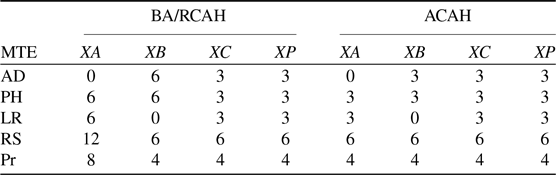
Following this strategy, the PePi metric was computed for PH, AD, Pr and LR MTEs; Table 5 shows the total PePi attack numbers for the whole MTEs flown with ACAH and BA/RCAH configurations. The PePi attack breakdown w.r.t specific phases in these MTEs are tabulated in Appendix B.
Total PePi attack numbers for ADS-33 MTEs
We return to the investigation of the PePi normalisation by examining its correlation with the HQRs awarded by the pilots in flight and simulation tasks in Section 4. For the PePi metric control accumulation, the A
ηG
and A
ηS
calculated individually for each control (XA, XB, XC and XP) are averaged to obtain a single combined mean value (Equation (4)), $\overline {{A_{\eta G}}} $
and
$\overline {{A_{\eta G}}} $
and $\overline {{A_{\eta S}}} $
, for comparisons with HQRs.
$\overline {{A_{\eta S}}} $
, for comparisons with HQRs.
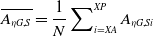 \begin{align}\overline {{A_{\eta G,S}}} = \frac{1}{N}\mathop \sum \nolimits_{i = XA}^{XP} {A_{\eta G,Si}}\end{align}
where i corresponds to the four (XA, XB, XC and XP) controls and N is the number of controls.
3.3.3 Cut off Frequency (CoF) metric
The CoF metric as defined in Section 2 is the frequency at which 70% of the control displacement (50% of control power) signal has combined when represented as a gain in the frequency domain [Reference Blanken and Pausder20, Reference Tischler and Remple21]. It is particularly meaningful when the pilot is acting to correct errors from the intended performance in the presence of a random disturbance. Figure 10 illustrates the CoF method in an outer plot (right), in combination with the composite TFD-A ηR metric plots (Fig. 8), for a PH MTE flown in the ASRA using the BA configuration. The plot shows a ratio between the control input amplitudes summed up to the current frequency (Ση) and the amplitudes summed over the full frequency range (Ση TOT ). The CoF is the frequency at which this ratio is 0.7.
CoF and composite TFD-AηR metric plots for lateral cyclic control activity.

The CoF is calculated using the frequency interval 0.2–2Hz; the lower limit largely removing the lower-frequency guidance element of the control activity from the analysis, and the upper limit removing artefacts (e.g. measurement noise, digitisation, and pilot inceptor dynamics [Reference Tritschler, O’Connor, Holder, Klyde and Lampton12]) introduced in the time-frequency domain transformation [Reference Perfect, Gubbels, White, Padfield and Gubbels2]. Figure 10 shows the CoF metric calculated for the whole PH MTE as 0.6Hz and for the 30s final hover-stabilisation phase as 0.7Hz; so, 16% higher frequency content in the last 30s of the MTE compared to the whole MTE. The A ηR loc increases from the start to the end of the MTE.
In this section, the utility of the CoF metric in understanding the pilot control compensation is demonstrated. However, with its focus on discrete events, the attack metric exposure reflects pilot control compensation better for the complex multi-axis MTEs. The application of the combined adaptive A ηRC and PePi normalisation metrics are now demonstrated by examining the correlation with the HQRs awarded by the pilots for a range of MTEs with different task performance requirements and dominant control axes.
4.0 Correlation of compensation metrics with HQRS
In this section, two case studies, one from flight, the other from simulator tests, performed by the same pilot (Pilot A), are discussed in more detail to demonstrate the application of the developed metrics and the TFD-A ηR loc composite-charts, and correlation with the HQRs awarded by the pilots. Within each of these cases, different MTEs with different task performance requirements and dominant control axes have been examined. The same analysis is presented for the results obtained from Pilot B in Appendix C.
4.1 Attack activity rate metric
4.1.1 Case study 1: Flight test
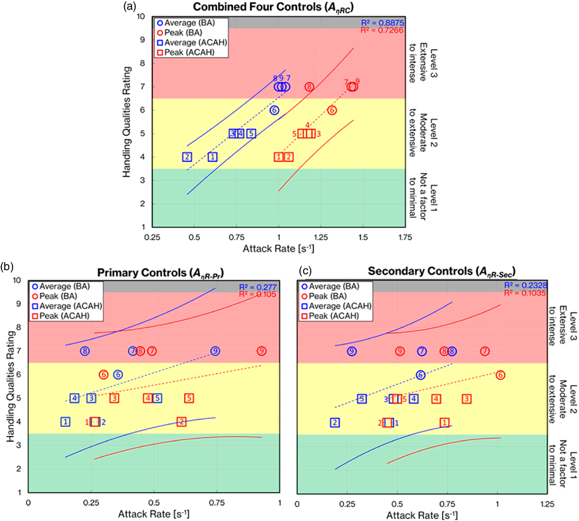
Flight test data gathered for five different MTEs (PH, AD, Pr, LR and RS) flown in the ASRA using the BA and ACAH configurations are assessed (see Table 6). For each case, Table 6 compares the key predicted HQs feature and level with the assigned (pilot) HQs level, rating and experience, and the associated peak phase(s) captured from the A ηR loc metric. Comparisons of the adaptive A ηRC metric with the HQRs are presented in Fig. 11, showing results for all four controls combined, and separated primary and secondary controls. Each plot shows the average and the peak A ηR results. Within the figures, the data points are identified with a unique number that corresponds to the specific test case (i.e. MTE and configuration), given in Table 6. The best fit straight-line (dashed) between the HQRs and A ηRC , are shown, along with the coefficient of determination (r 2 ), and 90% prediction-boundary calculated using the T-distribution [Reference Navidi33]. The coloured regions differentiate the HQ levels from the HQR scale, with the associated compensation descriptors on the secondary Y-axis.
Details of the cases presented in Fig. 11 (pilot A in ASRA)

HQR vs peak and average AηR for (a) Combined, (b) Primary and (c) Secondary controls (Pilot A: Flight Trial).

The first observation is that all results lie in the HQ Level 2 range. The second is that for three of the four MTEs flown with the BA were awarded HQR 6. Third, within this seemingly narrow band, the A ηR more than doubles, when viewed as the average or peak. Of course, Level 2 is not a narrow band; rather it covers the range from desired performance achieved with moderate compensation to adequate performance achieved with extensive compensation. The change from desired to adequate performance within this band is significant in terms of the expected relationship between the HQR and any compensation metric. It is likely to be nonlinear and the results do suggest this. Figure 11(a) shows a reasonably positive correlation between the HQRs and A ηRC, with the A ηRC avg showing the highest r 2 value of 89%, with the narrowest spread and the prediction boundary amongst all the cases. The correlations for separated primary and secondary controls are lower. This can partially be explained by the different sources of deficiency and consequent compensation in the different MTEs for the same HQR. For example, in Case 8 (LR, BA) the dominant compensation was from the secondary controls (e.g. XB); for Case 9 (PH, BA) the dominant compensation was from the primary controls (XA, XB). The combined peak A ηR is similar (1.6–1.8) so reflecting the different contributions to overall compensation.
The separation of the controls into primary and secondary is found to be important for understanding the respective contribution of each to the corresponding A ηRC values since, within each of these MTEs, different controls will be dominant during different phases of the MTEs. To illustrate this, two cases; (1 (AD-ACAH) and 9 (PH-BA)) have been selected from the two extreme HQ rating groups (4 and 6) to represent the moderate and extensive levels of control compensation, where the pilot commented the workload to be tolerable for Case 1 and extremely high for Case 9.
Case 1 is the AD MTE flown with the ACAH configuration and awarded an HQR 4 by the pilot. Figure 11(a) shows that the A ηRC pk is almost double the A ηRC avg . This is dominated by the secondary controls where the difference between the A ηR-Sec pk and A ηR-Sec avg is almost 0.7/s, whereas, in the primary controls, the difference between the A ηR-Pr pk and A ηR-Pr avg is <0.1/s. Between primary and secondary controls, the latter dominates; the A ηR-Sec pk being almost double the A ηR-Pr pk . The pilot commented that he applied “at least moderate compensation particularly in the off-axis channels”. From the TFD-A ηR loc charts shown in Fig. 12, the peaks largely occur during the stabilised hover capture phase with peak A ηR loc > 1.5/s in XA and XP. The pilot commented that due to the poor engine governing dynamics, the control strategy had to be modified slightly from his usual accel/decal strategy. The spectrograms also indicate that there is a hot-spot in the low-frequency region below 0.2Hz in the four controls, which corresponds to the guidance frequency range and reducing significantly at higher frequencies; as expected the guidance-maximum is in the primary XB control.
TFD-AηR loc composite plots for case (1, AD-ACAH), HQR 4.

Case 9 is the PH MTE flown with the BA configuration and awarded an HQR 6 by the pilot. Compared to the previous case, the overall control compensation is much higher, as shown in Fig. 13. The primary controls, XA and XB, are dominant, with A ηR-Pr 2.5–3 times the A ηR-Sec , for both average and peak values. The TFD-A ηR loc plots for the primary controls show A ηR loc increasing from the start to the end of the MTE, with a peak of 3/s in XB at the end of the stabilisation period. The pilot commented that he “cannot relax at any point during the manoeuvre”. Although the pilot commented that “the task required compensation in all axes continuously”, the TFD-A ηR loc plots show the dominant primary controls, with A ηR for XB remaining above 2/s throughout the MTE. The A ηR loc for XC remains around 1/s and XP remains below 2/s in the initial and final phases with a dip during the hover capture phase for XP. The TFD-A ηR loc also shows high-frequency content in all the controls throughout the MTE. However, at a high-frequency range (>0.5Hz), the amplitudes are lower in secondary controls compared to the primary. For this case the pilot commented that “accuracy was inconsistent, chasing the aircraft rather than controlling it”, “poor stability created issues in pitch, roll and yaw” and “the level of precision could be achieved but the workload was extremely high throughout the MTE”.
TFD-AηR composite plots for case (9, PH-BA), HQR 6.

4.1.2 Case study 2: Simulator test
The same aircraft configurations i.e. BA and ACAH, and MTEs, were flown in HELIFLIGHT-R by the same pilot and the results are shown in Table 7 and Fig. 14(a), (b) and (c). It is noted that the A ηR values are lower, and the gradient of variation with HQR is steeper than in the ASRA flights (Fig. 14(a) compared with 11(a)). Also, the awarded HQRs extend into the Level 3 region. Again, in this section, two different HQR cases 1 and 9 have been selected from two extreme HQ rating groups (i.e. 4 and 7) to represent the moderate and maximum tolerable levels of pilot control compensation.
Details of the cases presented in Fig. 14 (pilot A in Simulator)

1 Note that roll from pitch cross coupling is predicted as level 2 for forward flight.
HQR vs peak and average AηR for (a) Combined, (b) Primary and (c) Secondary controls (Pilot A: Simulator Trial).
As in the flight test, the A ηRC results show a strong level of overall correlation (Fig. 14(a)). However, for the primary and secondary controls (Fig. 14(b) and (c), respectively), the correlation is much lower. As in flight test cases, the BA and ACAH configurations are separated in the HQR levels. The BA configurations are located in the top-right region of the band with the expected higher levels of control compensation (and HQRs ≥ 6). The ACAH configurations are located in the bottom-left region with correspondingly lower levels of pilot compensation (and HQRs ≤ 5). However, when separated into primary and secondary controls, these regions are not as clearly distinguished as with all four controls combined. As discussed for the ASRA data, this is due to the way the compensation is distributed amongst the four controls.
Case 1 is the LR MTE flown with the ACAH configuration and awarded an HQR 4. Compared to the HQR 4 case in the flight test (Fig. 12), the level of compensation as calculated by the TFD-A ηR loc is lower. For the LR MTE, the A ηRC Pk is 1.6/s in flight for the ACAH, compared with 1.0/s in simulation; 2.1/s compared with 1.2/s for the BA configurations. In this case, the secondary controls are dominant with A ηR-Sec almost three times the A ηR-Pr , for both average and peak results. The TFD-A ηR loc plots in Fig. 15 provide insight into these differences by showing that, among the three secondary controls, XB and XP appear to have higher peak A ηR loc > 1/s, whilst for XC, the A ηR loc remains <1/s throughout. As in the flight test Case 1, the primary control shows a large low-frequency hot-spot <0.2Hz, which drops at higher frequencies. This low-frequency peak is, again, attributed to the guidance frequency corresponding to the core task frequency. From the control activity and TFD charts, the pilot was active in XB throughout the MTE having peak A ηR loc occurring during the translation phase, while for all the rest of the controls the peaks occurred during the hover capture phase. The pilot commented that “the most difficult element of the task was the longitudinal position keeping”. This was predominantly due to poor outside visual cues in the simulation environment, which in the LR MTE, dominates the pilot’s control strategy. During the assessment of the visual cueing, it was found that due to the hardware limitations, rich textural environment (close to the real-world) could not be fully recreated. This restricted the ability of the pilot to apply accurate translational rate and attitude corrections [Reference Perfect, Gubbels, White, Padfield and Gubbels2].
TFD-AηR loc composite plots for case (1, LR-ACAH), HQR 4.

Case 9 is the PH MTE flown with the BA configuration and awarded an HQR 7. Figure 14(b) and (c) show that the dominant controls are primary, with the A ηR-Pr being 2–3 times the A ηR-Sec , for both average and peak results. Expanding on this using the TFD-A ηR loc plots in Fig. 16, the A ηR loc peaks to 2/s in XA, while for XB it remains ≥1/s throughout. The TFD plots show consistent high-frequency content with multiple peaks around 0.4–0.6Hz for these controls. The pilot commented that “there were continuous control perturbations, the aircraft was easy to excite and never truly stabilised in the hover”. This can be seen from XA and XB control activity having continuous compensation at the hover spot in the last 30s window. The XA plot clearly shows the level of compensation in capturing the hover point (between 18 and 20s) and throughout the 30s hover (20–50s). This is captured as a ramp in the A ηR loc and the first hot-spot in the TFD spectrogram. At the same location in time, hot-spots are shown in XB and XC with A ηR loc s. In this case, the aircraft model was predicted to have Level 2 stability, which required the pilot, during testing, to use maximum tolerable compensation in all axes and is reflected in the spectrograms.
TFD-AηR loc composite plots for case (9, PH-BA), HQR 7.

4.2 Perfect pilot: guidance and stabilisation
Using the PePi normalisation to estimate the distribution of G&S in the control attack, Fig. 17(a) shows the mean guidance attack $\overline {{A_{\eta G}}} $
and Fig. 17(b) shows the mean stabilisation attack
$\overline {{A_{\eta G}}} $
and Fig. 17(b) shows the mean stabilisation attack $\overline {{A_{\eta S}}} $
, for combined controls (Equation (4)). The unique data point numbers correspond to the specific test cases defined in Tables 6 and 7 for flight and simulator test, respectively. In a rather curious result, the guidance attack shows a negative trend with HQRs, whereas the stabilisation attack shows a positive trend; for flights in ASRA and HELIFLIGHT-R. The result is explained by considering the increase in compensation is largely due to stabilisation as task difficulty increases. In terms of the correlations, as observed in the separated primary and secondary controls in the previous section, the separated guidance and stabilisation attacks also show weak correlation with HQRs. The separated PePi guidance and stabilisation attack metric has been introduced to further understand the pilot control compensation and its contribution to the task performance, by assessing the relative strength of each to the overall pilot control activity.
$\overline {{A_{\eta S}}} $
, for combined controls (Equation (4)). The unique data point numbers correspond to the specific test cases defined in Tables 6 and 7 for flight and simulator test, respectively. In a rather curious result, the guidance attack shows a negative trend with HQRs, whereas the stabilisation attack shows a positive trend; for flights in ASRA and HELIFLIGHT-R. The result is explained by considering the increase in compensation is largely due to stabilisation as task difficulty increases. In terms of the correlations, as observed in the separated primary and secondary controls in the previous section, the separated guidance and stabilisation attacks also show weak correlation with HQRs. The separated PePi guidance and stabilisation attack metric has been introduced to further understand the pilot control compensation and its contribution to the task performance, by assessing the relative strength of each to the overall pilot control activity.
HQR vs mean AηG and AηS plots (a) Guidance; (b) Stabilisation (Pilot A: Flight and Simulator).

Comparing the two extreme ASRA cases, Case 2 actually shows slightly higher guidance. The HQR awarded for this case was 4, moderate pilot compensation. The pilot commented “relatively large stick displacements were required to generate the attitude changes,” but “workload was only moderate”. At the other extreme, Case 9 shows a dominating 95% stabilisation. The HQR awarded for this case was 6, extensive pilot compensation, with the pilot commenting that, “the task required compensation in all axes continuously”.
Considering the extreme simulation cases, for Case 5, the $\overline {{A_{\eta G}}} $
is 43% with HQR 5, considerable pilot compensation. The pilot in this case commented that “overall task performance was on the border between the desired tolerances and the adequate tolerances”. In contrast, Case 9 shows a
$\overline {{A_{\eta G}}} $
is 43% with HQR 5, considerable pilot compensation. The pilot in this case commented that “overall task performance was on the border between the desired tolerances and the adequate tolerances”. In contrast, Case 9 shows a $\overline {{A_{\eta S}}} $
of 90%, with HQR 7, maximum tolerable pilot compensation. The pilot in this case commented that “the aircraft was never truly stabilised at the hover point” and thus required considerable pilot compensation. These results suggest a relationship between the metric levels and the compensation descriptors.
$\overline {{A_{\eta S}}} $
of 90%, with HQR 7, maximum tolerable pilot compensation. The pilot in this case commented that “the aircraft was never truly stabilised at the hover point” and thus required considerable pilot compensation. These results suggest a relationship between the metric levels and the compensation descriptors.
5.0 Subjective vs objective metric boundary
The previous section assessed the flight and simulator test data from Pilot A. During the LS project, most of the MTEs were flown by a second pilot (Pilot B) in both flight and simulation. The analysis used in the previous sections has also been applied to the Pilot B data as shown in Appendix C.
By collating the HQR vs A ηRC Pk results from both Pilot A and B, new HQR-A ηR Compensation Level (CL) boundaries can be postulated, specifying two levels of control compensation, as shown in Fig. 18. Figure 18(a) shows the A ηRC pk metric against HQRs for the ASRA flight tests, while Fig. 18(b) shows the same for the HELIFLIGHT-R flight tests.
HQR-peak AηR boundaries for combined four controls (a) Flight-AηRC pk and (b) Simulator- AηRC pk.

In all the charts, the HQR boundary limits for CL1 and CL2 boundaries correspond to the transition point between Level-1 and 2 HQRs. The A ηRC pk boundary limits are based on the maximum HQR-A ηR combination obtained within each case. For the ASRA cases, the A ηRC pk CL1 boundary corresponds to Pilot B, Case 1, having A ηRC pk of 0.7/s, while the CL2 boundary corresponds to Pilot A, Case 9, having A ηRC pk of 2.3/s. For the HELIFLIGHT-R cases, the A ηRC pk CL1 boundary corresponds to Pilot B, Case 2, having A ηRC pk of 0.6/s, while the CL2 boundary corresponds to Pilot A, Case 9, having A ηRC pk of 1.3/s. The solid line passing through the data points is the regression trend line and the parallel dotted lines represent ±1 HQRs spread. Most of the data points fall within this tolerance.
The CLs from the ASRA tests are noticeably higher than those from the HELIFLIGHT-R tests. Moreover, the correlation in the flight trial is stronger than that in the simulator, for Pilot A and B combined. Considering the attack metric as a measure of control compensation this result suggests that pilots, at least the two involved in the LS trials, tolerate a higher workload in flight for a given Level 2 HQR. A related interpretation is that the generally poorer visual cues in the simulator (as noted in Ref. (Reference Perfect, Gubbels, White, Padfield and Gubbels2)) led to pilots exceeding the adequate performance standard at the lower attack activity rate; because, without sufficient fine texture cues, increasing the attack activity rate would not result in productive closed-loop control. Extending this reasoning, the improved surface visual cues in flight gave the pilots confidence to increase the attack activity rate to maintain adequate performance. The data suggest that the pilots are applying at least moderate control compensation at the CL1 boundary for both flight and simulator. At the CL2 boundaries, the pilots are applying at least maximum tolerable control compensation (HQR 7) with A ηRC pk >2.3/s in flight and >1.3/s in the simulator. We have hypothesised a visual-cue related explanation for why the pilots were prepared to accept higher levels of control compensation in flight test than in the simulator for a given HQR. However, during the LS trials this question was not specifically addressed, and the result warrants further investigation.
6.0 Guidelines for attack metric derivation and application
The approach taken in the analysis described above has evolved into a systematic process for deriving the attack-based control compensation metric. The steps below summarise this process, which can be used as guidelines for pilot compensation assessment.
-
(a) Determine an appropriate control threshold value to capture productive control inputs representing G&S control activity. The appropriate threshold can be determined from the initial run-in to the MTE.
-
(b) Select the window width for time-varying attack segmentation through the MTE. To develop representative composite TFD-A ηR exposure, the suitability of the selected window should be assessed in conjunction with the spectrograms, formulated to highlight features of the control signal.
-
(c) Derive the average and peak A ηR for each MTE; the peak values should be used as the CCM.
-
(d) The PePi attack pattern should be defined for the guidance control inputs for each of the MTEs to enable control activity to be separated into G&S activity.
-
(e) The combined attack for primary and secondary controls, computed based on the weighted-adaptive algorithms (Equations 2 and 3), are computed to provide the strongest correlation with the HQRs awarded by the pilot.
-
(f) The TFD spectrograms are created by calculating the STFT of the control signal plotted as a contour-plot against time and time-localised frequency. The moving window width should be selected to provide resolution in both time and frequency that highlights key features of the control signal.
-
(g) In defining the compensation level boundaries, the selection of the A ηr limits should be based on the maximum HQR-A ηR combination point falling inside the ±1 HQR tolerance.
7.0 Conclusions and future work
The paper has described the development of a new control compensation metric, suitable for predicting and explaining the handling qualities rating assigned by a pilot. The weighted adaptive attack activity rate metric has been shown to have good correlation with the handling qualities ratings awarded by pilots for a range of mission task elements. The following are the key conclusions drawn from this work:
-
1. A 2.5% control attack threshold was found to be appropriate to remove unproductive control deflections, without changing the trends in the overall metrics.
-
2. Time, or MTE-phase, based segmentation of the attack metrics has been shown to be essential to capture the peak compensation zones within different phases of the MTE where the pilot is working the hardest.
-
3. The peak attack metric has the strongest correlation with the HQR for an MTE. A combined average attack metric, and average-HQR, masks compensation peaks which weakens the correlation with the subjective assessments.
-
4. The combination of the time-frequency domain spectrograms with the localised time-varying attack activity rate metric provides detailed insight into the pilot compensation within different phases of the MTEs.
-
5. The combined weighted adaptive attack activity rate metric, for all four controls, has shown a strong correlation with the HQRs when applied to the range of MTEs. Results for separated primary and secondary controls show much weaker correlation with HQRs. However, separation is useful in understanding the different contribution of each control.
-
6. To further understand pilot control compensation and its contribution to the task performance, the perfect-pilot, or PePi, technique has been introduced to extract the relative strength of guidance and stabilisation contributions from within the overall pilot control activity.
-
7. By combining the weighted adaptive peak attack activity rate metric for a range of MTEs and both pilots, new compensation level boundaries have been proposed. It was found that the pilots were prepared to accept and manage a higher level of control compensation in flight than in the simulator for a given HQR. We have hypothesised that this might be due to pilots able to close control loops more tightly in flight due to improved visual cueing. Further research is required to explore and fully understand these differences.
The results presented in this paper are based on a relatively limited number of tests and further investigations are required to refine the metric and the proposed compensation boundaries. The utility of the proposed metrics in understanding pilot adaptation and associated simulation fidelity will be explored. Moreover, the PePi concept, theoretically based on the MTE task performance strategy and requirement, will be extended using analytical pilot modelling techniques.
Acknowledgements
The UK’s Engineering and Physical Sciences Research Council (EP/P031277/1 and EP/P030009/1) funded the research reported in this paper. The work was carried out using the flight and simulator test data gathered during the Lifting Standards (EP/G002932/1) project. The use of the NRC’s Bell 412 ASRA facility is gratefully acknowledged and special thanks to the test pilots who participated in the trails.
Appendix A. Mission Task Elements (Cargo/Utility, Good Visual Environment)
Precision Hover (PH) MTE definition

Pirouette (Pr) MTE definition

Lateral Repositioning (LR) MTE definition

Acceleration Deceleration (AD) MTE definition

Roll-Step (RS) MTE definition

Appendix B. PePi metric phase-wise breakdown of ADS-33 MTEs
Precision Hover (PH) task PePi phase-wise breakdown

Acceleration Deceleration (AD) task PePi phase-wise breakdown

Lateral Reposition (LR) task PePi phase-wise breakdown

Pirouette (Pr) task PePi phase-wise breakdown

Appendix C. Lifting Standards (LS) Pilot B
Details of the cases presented in Fig. C1

HQR vs peak and average AR estimations for (a) Combined, (b) Primary and (c) Secondary controls (Pilot B: Flight).

HQR vs peak and average AR estimations for (a) Combined, (b) Primary and (c) Secondary controls (Pilot B: Sim).

Details of the cases presented in Fig. C2


 Open access