





1. Introduction
Glacier surging is a quasi-periodic phenomenon of glacier dynamics where glaciers experience sudden short periods of accelerated flow followed by longer periods of stagnation (Meier and Post, Reference Meier and Post1969). These events significantly alter glacier geometry and mass distribution, and can pose hazards near populated areas by initiating glacier outburst floods (Vale and others, Reference Vale, Arnold, Rees and Lea2021; Kumar and others, Reference Kumar, Rana, Mehta and Rawat2024). Heavy crevassing, along with significant mass transfer and rapid surface velocity increases, are important signals of surge activity (Sund and others, Reference Sund, Eiken, Hagen and Kääb2009; Kääb and others, Reference Kääb, Bazilova, Leclercq, Mannerfelt and Strozzi2023). Glacier surges are clustered geographically, and one of these significant clusters is the archipelago of Svalbard (Jiskoot and others, Reference Jiskoot, Murray and Boyle2000). There are several existing theories as to why glaciers surge (Kamb and others, Reference Kamb1985; Fowler and others, Reference Fowler, Murray and Ng2001; Benn and others, Reference Benn, Fowler, Hewitt and Sevestre2019; Thøgersen and others, Reference Thøgersen, Gilbert, Schuler and Malthe-Sørenssen2019), but despite efforts to monitor and understand this phenomenon, we are still unable to fully explain the required conditions for their occurrence, or predict future active surge phases, proving that this phenomenon and its triggers remain poorly understood. Especially in a warming climate, where glaciers contribute to rising sea levels (IPCC, 2023), it is important to monitor and understand dynamic instabilities like surges further (Lovell and others, Reference Lovell2026).
Studying glacier surges has become easier with the increasing availability of remote sensing data. The existing automated and semiautomated methods for monitoring and detecting surges rely mainly on synthetic aperture radar (SAR) and optical satellite data. Existing methods include surface velocity tracking (Guillet and others, Reference Guillet2022; Paul and others, Reference Paul2022; Koch and others, Reference Koch, Seehaus, Friedl and Braun2023; Li and others, Reference Li, Chen, Mao, Yang, Chen and Cheng2024), changes in interferometric SAR coherence (Mannerfelt and others, Reference Mannerfelt, Schellenberger and Kääb2025), backscatter pointing toward the sudden crevassing (Kääb and others, Reference Kääb, Bazilova, Leclercq, Mannerfelt and Strozzi2023) and changes in albedo and terminus advance from optical data pointing toward mass transport (Herreid and Truffer, Reference Herreid and Truffer2016; Vale and others, Reference Vale, Arnold, Rees and Lea2021; Guillet and others, Reference Guillet2022; Ke and others, Reference Ke, Zhang, Fan, Zhou and Song2022), with the latter being effective mainly on debris-covered glaciers in High Mountain Asia. More recently, the detection of surges from a multi-method approach signifies a clear step forward, as different methods are powerful in different conditions. Guillet and others (Reference Guillet, Benn, King, Shean, Mannerfelt and Hugonnet2025) employed surface velocity, SAR backscatter and elevation change data to semi-autonomously detect surges globally. Their approach is based on a mix-of-experts approach where the majority (two out of three in their case) need to indicate surging for a safe detection, and this generic set-up is expandable for the future using more methods. Their elevation data are based on acquisitions from the TERRA Advanced Spaceborne Thermal Emission and Reflection Radiometer, which as of 2026 or 2027 will stop collecting data (Berthier and others, Reference Berthier2024). It is therefore essential to explore new methods of surge detection, especially from elevation data, to uphold this momentum in detection improvements.
Elevation data have previously been used for surge detection on Svalbard and elsewhere (Sund and others, Reference Sund, Eiken, Hagen and Kääb2009; Guillet and others, Reference Guillet2022; Ke and others, Reference Ke, Zhang, Fan, Zhou and Song2022; Kumar and others, Reference Kumar, Rana, Mehta and Rawat2024). A typical signal before a surge is moderate thickening in the reservoir areas and thinning in the receiving areas. In contrast, a surging glacier demonstrates the opposite behavior: mass is rapidly transferred from the reservoir area toward the terminus, leading to pronounced elevation increases—often tens of meters—in the receiving area and corresponding thinning in the reservoir area (Wu and others, Reference Wu2024). This behavior forms the basis for the detection algorithm developed in this study.
With the launch of NASA’s ICESat-2 satellite in 2018, we now have access to spatially and temporally sparse, but accurate elevation data with seasonal repeat-tracks. ICESat-2 measures elevation along narrow tracks with very high precision, making it possible to detect the patterns of elevation gain and loss caused by surging. Using these data together with machine learning, we can look for these patterns automatically and more consistently. High-latitude regions like Svalbard—and more broadly the Arctic and Antarctic—have great potential for this approach, as the near-polar orbit of the satellite leads to dense repeated tracks near the poles. In contrast, in regions like High Mountain Asia, where track spacing is much wider, narrow glaciers may fall between the tracks, limiting the coverage and detection capability.
By focusing on elevation data from ICESat-2, our aim in this study is to add a new method of surge detection, which may contribute to a more robust understanding of glacier surges in the long term.
2. Data and methods
We trained a Random Forest (RF) (Breiman, Reference Breiman2001) classifier using labeled data from Kääb and others (Reference Kääb, Bazilova, Leclercq, Mannerfelt and Strozzi2023), which represents known surges in the area that exhibited strong crevassing visible from SAR backscatter changes. Our method detects surges based on elevation changes derived from ICESat-2 measurements, normalized using a reference digital elevation model (DEM). The aim was to differentiate between surging and non-surging glaciers by identifying elevation change distributions indicative of dynamic instabilities, rather than long-term thinning or mass balance trends.
2.1. ICESat-2
ICESat-2 (Ice, Cloud and Land Elevation Satellite-2) uses the Advanced Topographic Laser Altimeter System (ATLAS), a photon-counting laser altimeter operating at a wavelength of 532 nm (Neumann and others, Reference Neumann2019). ATLAS emits 10 000 pulses per second across 6 beams arranged in three beam pairs, each consisting of a strong and a weak beam, providing accurate surface height measurements (Neumann and others, Reference Neumann2019). All six beams were used in this study. Within each beam pair, the across-track separation is  $\sim$90 m, while the two pairs are separated by $\sim$3.3 km along-track, providing detailed spatial coverage of glacier surfaces. The system provides a vertical accuracy of $ \lt $10 cm and a spatial resolution of $ \lt $6.5 m (Markus and others, Reference Markus2017; Magruder and others, Reference Magruder, Neuenschwander and Klotz2021; Martino and others, Reference Martino, Itzler, McIntosh and Bienfang2023), with a 91 day repeat track over polar regions, allowing for highly accurate seasonal measurements of glacial surfaces (Neumann and others, Reference Neumann2019). Data quality is influenced by cloud cover, which is a major factor for uncertainty in the method. In combination with the 91 day repeat cycle, this means that data are in practice only reliably available on yearly time scales, and some years may be covered more or less than others.
We utilized Version 5 of the Level-3A ATL06 Land Ice Height product (further referred to as ATL06), which offers measurements of surface elevation with 20 m along-track spacing (Smith and others, Reference Smith2019). Data spanning 2018–23 were used to derive surface elevation changes.
2.2. Other data
Regional DEMs from the Norwegian Polar Institute (2014) were used as a reference for computing elevation changes. The DEMs are based on aerial photographs acquired mainly between 2008 and 2012, with one small area from 1990 (non-glaciated area) and another from 2021 (covering a few glaciers). All images were collected during the ablation season (mid-July to mid-August), ensuring minimal snow cover. The DEMs are referenced to orthometric heights derived from ground control points, and they have an overall vertical accuracy of about 1–2 m, although regional biases may occur. Since glacier surges typically involve elevation changes of several tens of meters, no further corrections were applied.
Glacier outlines were obtained from the Randolph Glacier Inventory (RGI) Version 7.0 (RGI Consortium, 2023) for spatial data organization.
The training dataset for the RF classifier consisted of 25 glacier surge events between 2017 and 2023 identified by Kääb and others (Reference Kääb, Bazilova, Leclercq, Mannerfelt and Strozzi2023) using SAR backscatter data. Non-surging glaciers were manually selected from glaciers with no surge detection in literature.
2.3. Feature extraction
Elevation changes were computed by differencing ICESat-2 elevations from the reference DEM:
 \begin{equation}
\Delta h = h_{DEM} - h_{ATL06}
\end{equation}
\begin{equation}
\Delta h = h_{DEM} - h_{ATL06}
\end{equation}Using RGI outlines, elevation change data were grouped by glacier, covering 1665 glaciers in Svalbard. We found that the ATL06 cloud mask often misclassified valid points near surging glacier termini and elected not to use it. Outliers were filtered using a Random Sample Consensus (RANSAC) approach (see Supplement Fig. S1), preserving meaningful elevation signals while reducing noise. A quality flag (good/poor) was assigned to each unit based on data completeness, with 502 glaciers (94.93% of Svalbard’s glacier area) labeled as good quality. The quality flag was assigned based on the number and spatial distribution of ICESat-2 ATL06 elevation points to ensure the reliability of results. Glacier units were labeled as good quality (QF = 1) if they contained at least 1500 elevation data points in total and a minimum of 500 points within the lower 40% of the glacier area (by elevation). The elevation data points refer to ICESat-2 ATL06 measurements, and the thresholds were applied to the combined dataset covering the entire 2018–23 study period. Units that did not meet both of these criteria were labeled as poor quality (QF = 0). In our dataset, the smallest glacier classified as good quality has an area of 1.04 km2 (GLIMS ID G014162E77518N), while the smallest glacier included overall has an area of 0.05 km2 (GLIMS ID G015353E79064N). This ensured that both the overall coverage and the spatial distribution of elevation data points—particularly in the lower glacier regions—were sufficient. Thresholds were chosen based on practical considerations and data inspection, with the lower 40% used as an approximation for the receiving area, where elevation changes during surges are typically most pronounced.
We ran our analysis over two different time scales. First, we used the full ICESat-2 dataset (2018–23) as one timestamp and compared it to the reference DEM (2008–12) to maximize the point density. Then, we attempted a yearly timescale to obtain more information within the ICESat-2 time period. For this yearly time scale, we used the hydrological year, which is 3 months ahead of the normal calendar year; starting at 1 October and ending at 30 September. The latter means predicting a surge/no-surge flag on 8330 glacier-year units between 2018 and 2023. A separate annual quality assessment labeled 1101 glacier-year units as good quality, considering the same criteria.
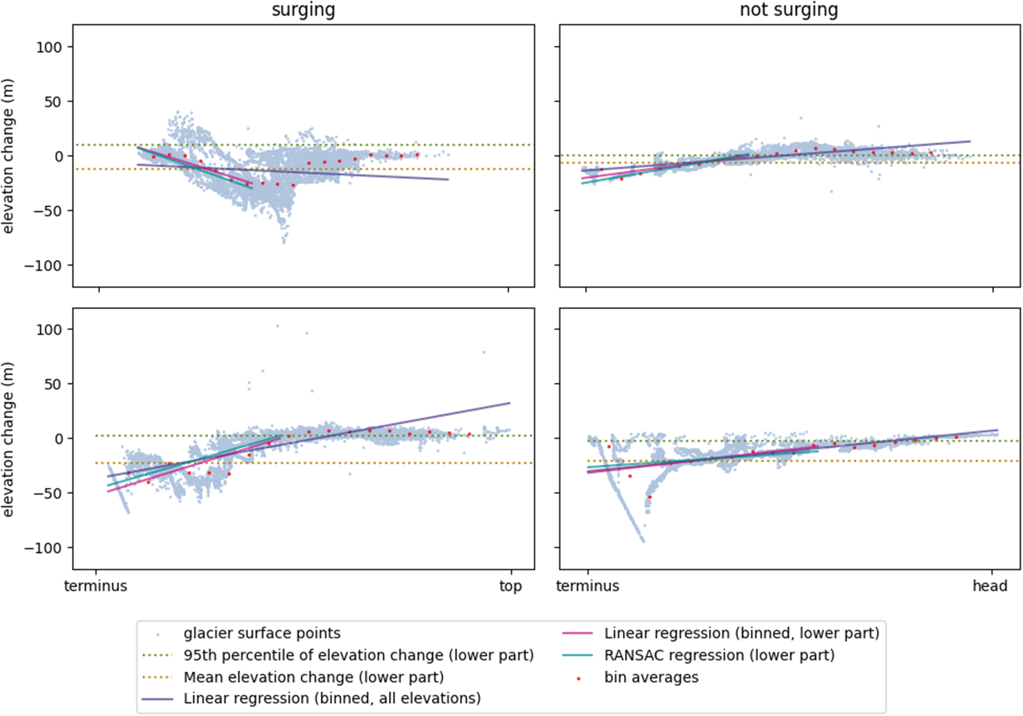
We evaluated the ICESat-2 point data through its hypsometric distribution for each glacier (Fig. 1). We used a hypsometric binning approach because it preserves the critical elevation-dependent patterns of a glacier surge and provides a consistent representation of the irregular ICESat-2 point data. This gives each elevation bin of the glacier the same weight; otherwise, the results would be affected by the number of points in each bin. The binning approach also makes the data more comparable between years. Each glacier was divided into two sections: the lower 40% and the upper 60% by elevation. For the lower section, we calculated linear and RANSAC regression coefficients and the mean and 95th percentile elevation change. Elevation bins (20 equal intervals, see Fig. S2) were used to examine elevation change trends across the glacier surface. Additional metrics included mean elevation change per bin, regression trends across bins, number of points exceeding a +15 m elevation change threshold in the lower section, and standard deviation and residuals from regression models. A total of 38 statistical features were extracted to characterize the elevation change distribution. These features were used as input for the RF classifier. We describe all features in the supplementary material (see Figs S3–S13 ), but the ones with the highest statistical significance are presented here.
Differences in elevation change distribution and statistical features used for classification for four glaciers: Nathorstbreen (a) and Osbornebreen (b), which were surging, and Bakaninbreen (c) and Olsobreen (d), which were not surging. Elevation changes represent the difference between DEM elevations from 2008 to 2012 and ICESat-2 elevations acquired during 2018–2024.

2.4. Model training and evaluation
The RF classifier was trained using 71 surging and 97 non-surging glacier units (see Tables S2 and S3 and Figs S14 and S15). The dataset was split into 70% training and 30% testing data using a stratified random split. The RF classifier (scikit-learn implementation) was trained using 100 decision trees, with a maximum depth of 80 and a minimum of 20 samples per split. Bootstrapping was enabled, meaning each tree was trained on a random sample (with replacement) of approximately 63% of the training data. To assess stability, the model was trained five times with different random seeds. Final predictions were obtained by majority voting across these five runs, and the mean predicted probability was also recorded. The output included binary class labels (surging/non-surging) and associated classification probabilities. Standard classification metrics, including accuracy, precision, recall, F1-score and the area under the curve (AUC), were calculated to assess model performance. Manual validation was performed for glaciers flagged as surging and of good quality using (1) visual evaluation of elevation change plots, (2) Sentinel-2 satellite imagery, (3) NASA ITS_LIVE velocity data (Gardner and others, Reference Gardner, Fahnestock and Scambos2022) and (4) comparison with existing literature (Kääb and others, Reference Kääb, Bazilova, Leclercq, Mannerfelt and Strozzi2023; Koch and others, Reference Koch, Seehaus, Friedl and Braun2023). Data were also analyzed by hydrological year (2019–23), resulting in 8330 glacier-year units. A separate quality assessment labeled 1101 glacier-year units (81.32% of Svalbard’s glacier area) as good quality.
3. Results
3.1. Detected surges
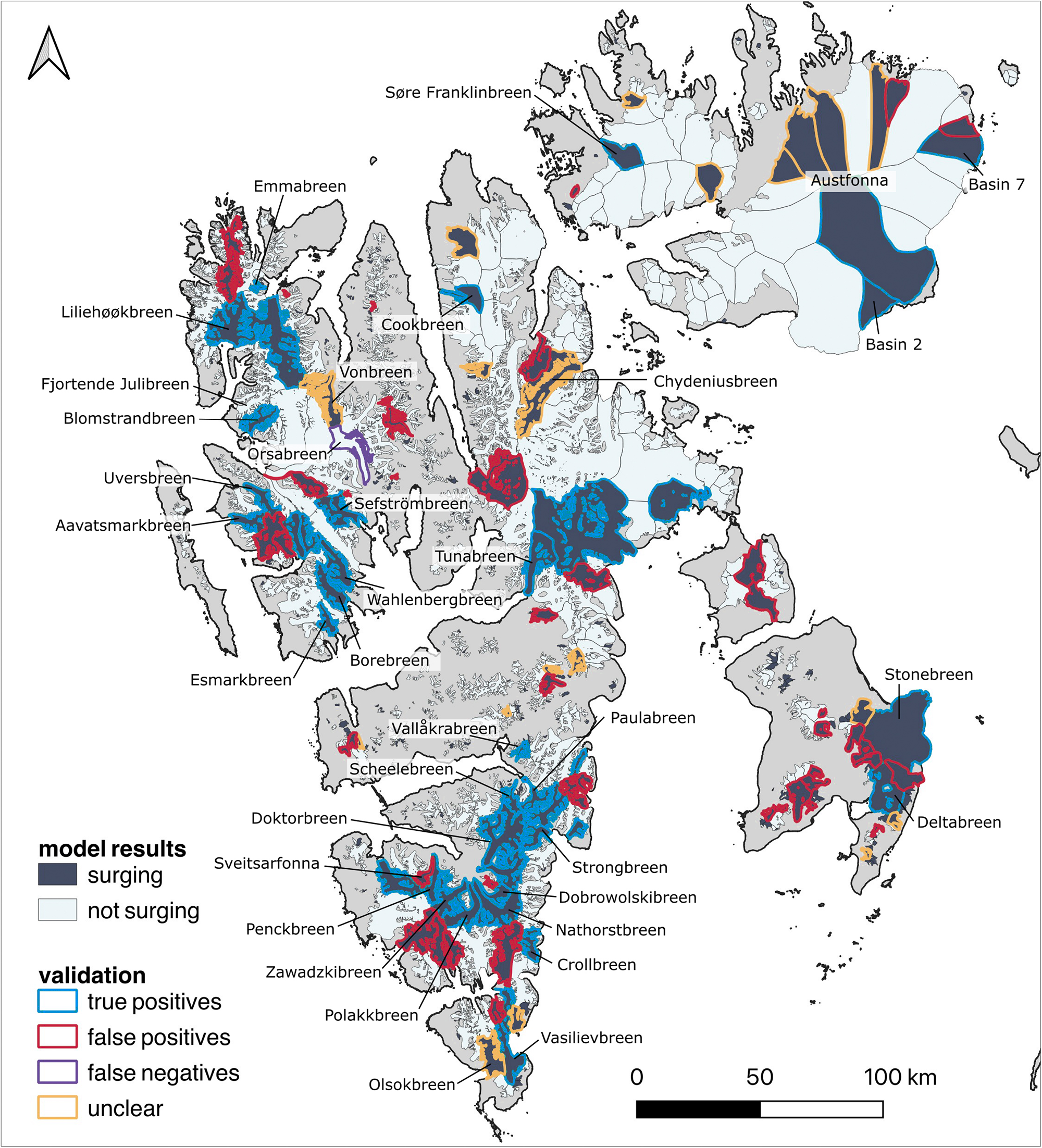
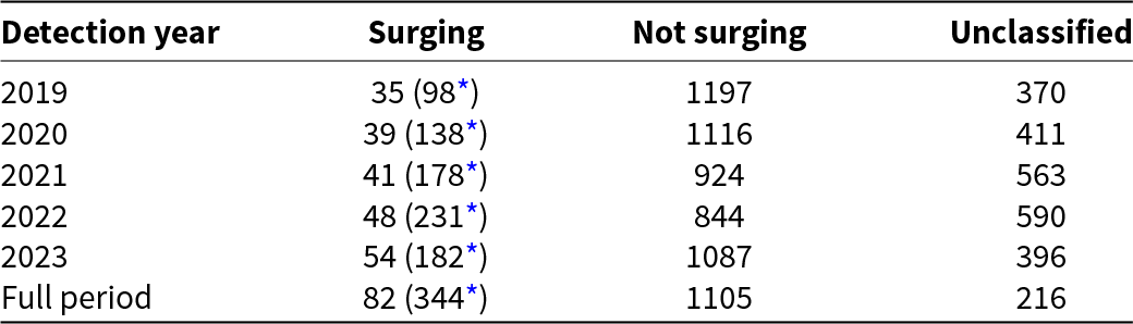
Using all available data from the 5-year period, 82 glaciers with a good quality flag were classified as surging, as shown in dark blue in Fig. 2, while 216 glaciers (13% by number) could not be classified due to insufficient data (Table 1). When the data were grouped by hydrological year, surges were detected for 216 corresponding glacier-year units on 77 unique glaciers. Combining both analyses, a total of 110 glaciers were classified as surging in at least one of the models. Of the 82 glaciers classified as surging in the full-period analysis, 49 were also detected in the hydrological-year analysis, allowing the surge onset year to be identified. Note that for glaciers that started surging prior to 2018, the exact surge onset date is unclear, and the first possible detection date of 2019 (the first hydrological year for ICESat-2; this accounts for 35 glaciers) is used instead.
Model results for 2008–23, indicating glacier surges starting or ending in that period.

Number of detected surges for each hydrological year (2018–23), based on elevation changes between the reference DEM (2008–12) and ICESat-2 data. Note that surges may have occurred any time between the reference DEM acquisition and the detection year. ‘Full period’ refers to the classification using the entire ICESat-2 record (2018–23). Unclassified glaciers are those with too few data points.

* Glaciers classified as surging with a poor quality flag.
Glaciers classified as surging and marked as good quality underwent manual validation. The models produced 48 false positives (red outline in Fig. 2) that could not be confirmed by external validation, and 20 of the glaciers labeled as surging only showed weak supporting evidence of a surge, these were marked as potential surges/unclear after manual validation (yellow outline in Fig. 2). Of the remaining 42 detected certain surges (green outline in Fig. 2), 20 were part of the training data, and 22 were new surges (high quality flag, externally validated and not part of the training dataset). These surges include six events that occurred during and 16 events outside the 2017–22 period analyzed by Kääb and others (Reference Kääb, Bazilova, Leclercq, Mannerfelt and Strozzi2023): 11 occurred before 2017 (2008–16), and 5 occurred after 2022.
The manually confirmed true positives include two surges that have not yet been described by other studies of recent surges: Crollbreen (surge start detected in 2021) and Søre Franklinbreen (surge start detected in 2020). The surge of these glaciers was confirmed through terminus advance on Sentinel-2 imagery, where Crollbreen has been advancing since 2017 and Søre Franklinbreen has advanced in 2018 and 2020. Historic surge advances of Søre Franklinbreen (Schytt, Reference Schytt1969) and Crollbreen (Lefauconnier and Hagen, Reference Lefauconnier and Hagen1991) had been used to incorporate both glaciers in existing surge inventories (e.g. Lovell and others, Reference Lovell2026). The remaining detected surges in this study have been described earlier: Blomstrandbreen and Comfortlessbreen (surge started in 2008, Sund and Eiken, Reference Sund and Eiken2010), the Nathorstbreen glacier system consisting of Nathorstbreen, Dobrowolskibreen, Zawadzkibreen and Polakkbreen (surge started in 2008/09, Sund and Eiken, Reference Sund and Eiken2010; Sund and others, Reference Sund, Lauknes and Eiken2014), Esmarkbreen (started advancing around 2010, Szafraniec, Reference Szafraniec2020), Stonebreen (surge started in 2012, Strozzi and others, Reference Strozzi, Kääb and Schellenberger2017; Guillet and others, Reference Guillet, Benn, King, Shean, Mannerfelt and Hugonnet2025), Aavatsmarkbreen and Wahlenbergbreen (surge started in 2013/14, Sobota and others, Reference Sobota, Weckwerth and Nowak2016; Sevestre and others, Reference Sevestre2018; Guillet and others, Reference Guillet, Benn, King, Shean, Mannerfelt and Hugonnet2025), Lilliehøøkbreen (surge started in 2014, Guillet and others, Reference Guillet, Benn, King, Shean, Mannerfelt and Hugonnet2025), Uversbreen (surge registered in 2014, Harcourt and others, Reference Harcourt2025), Emmabreen (surge registered in 2016, Harcourt and others, Reference Harcourt2025), Austfonna Basin 2 and Basin 7 (velocity increase in 2018, Zheng, Reference Zheng2022), Borebreen (surge started in 2023, Harcourt and others, Reference Harcourt2024; Guillet and others, Reference Guillet, Benn, King, Shean, Mannerfelt and Hugonnet2025), Doktorbreen, Sefströmbreen, Paulabreen and Deltabreen (surges started in 2024, Guillet and others, Reference Guillet, Benn, King, Shean, Mannerfelt and Hugonnet2025). Blomstrandbreen and the Nathorstbreen glacier system were described to surge before the study period of this paper began. Detecting surges on these two glaciers may indicate that the glaciers continued to accelerate throughout the beginning of this study period, or that a second active phase occurred between the DEM and ICESat-2 data acquisitions.
Using the full-period (2018–23) analysis, the model failed to detect six surging glaciers. Of these, five were detected as surging in at least one hydrological year, with two late-initiating surges (2023–24). Only Orsabreen (Koch and others, Reference Koch, Seehaus, Friedl and Braun2023) was not detected as surging in either the full-period or any hydrological-year analysis (purple outline in Fig. 2). A qualitative assessment from satellite images does not show other indications of surging (significant displacement or crevassing) at this glacier, and we thus assume that it may have been misclassified in the previous inventory. A detailed comparison of our results with previous studies is provided in the Supplement (see Tables S3 and S4).
3.2. RF model evaluation
The RF model was evaluated on a test set using standard classification metrics. For the 5 year dataset, it achieved an accuracy of 88.4%, with a high true positive rate and precision reflected in an F1-score of 87.8%. The AUC was 0.88, indicating very good accuracy. Feature importance analysis revealed that the most influential variables were the linear regression coefficient in the lower glacier part, residuals from the linear regression coefficient and averages of elevation change in bins 9 and 10 (covering middle glacier elevations, 40–50% of the individual elevation range).
4. Discussion
4.1. Surge detection
We note a general robustness in surge detection over the 10 year timespan between the reference DEM and the ICESat-2 archive. Using the entire ICESat-2 dataset for classification resulted in higher surge detection accuracy due to reduced noise and improved spatial coverage. However, this approach yields no information on the exact onset year. Classifying glaciers by hydrological year introduced more false positives but enabled the detection of smaller instabilities, such as surges that have just begun. For example, the surge of Borebreen, which started in 2023, was only visible in the yearly data series for that corresponding hydrological year.
Our analysis detected 42 manually validated surges between 2008 and 2023, which is more compared to previous studies (18 surges for 2015–21 by Koch and others, Reference Koch, Seehaus, Friedl and Braun2023; 25 for 2017–22 by Kääb and others, Reference Kääb, Bazilova, Leclercq, Mannerfelt and Strozzi2023; and 35 surges between 2000 and 2024 for Guillet and others, Reference Guillet, Benn, King, Shean, Mannerfelt and Hugonnet2025). This increase could be attributed to three key factors: (1) our longer study period compared to Koch and others (Reference Koch, Seehaus, Friedl and Braun2023) and Kääb and others (Reference Kääb, Bazilova, Leclercq, Mannerfelt and Strozzi2023) (2008–23), (2) different definitions and thresholds separating glacier instabilities from surges and (3) model and data limitations that lead to false positives. In addition to surges happening during the ICESat-2 data period, our method confirmed surges that happened between 2008 and 2019 (Nathorstbreen glacier system, Blomstrandbreen, Emmabreen) as well as surges beginning in 2023/24, such as Borebreen, Paulabreen and Deltabreen (Guillet and others, Reference Guillet, Benn, King, Shean, Mannerfelt and Hugonnet2025). We also identified smaller speedup events such as Stonebreen (Koch and others, Reference Koch, Seehaus, Friedl and Braun2023) and the Austfonna basin-7 (Zheng, Reference Zheng2022).
Some cases presented classification challenges. For example, Penckbreen’s surge extended into the RGI7 outline attributed to Sveitsarfonna, which led to the misclassification of Sveitsarfonna as surging. Other glaciers marked as potential surge/unclear showed elevation changes that look like a surge (positive elevation change at low altitudes), but were ambiguous from other satellite data. Many glaciers of the Austfonna ice cap show positive elevation change and advancing termini, but whether those are related to surges or the general positive mass balance anomaly of the region is still unclear (e.g., Morris and others, Reference Morris, Moholdt, Gray, Schuler and Eiken2022). Main causes of false positives were an outdated RGI glacier outline (see Fig. S16), cloud interference or steep slopes at glacier edges. False negatives can be caused by insufficient data coverage or by a small magnitude of the surge. Both Vallåkrabreen and Scheelebreen are missing in the results done by hydrological year due to insufficient annual data coverage.
4.2. Methodology
Using a DEM from 2008 to 2012 as a reference DEM introduced limitations: (1) surges detected in early years (e.g., 2019) could have occurred at any point after 2008, reducing temporal resolution, and (2) a global application is complicated by the need for high-quality region-specific DEMs. For future implementations in other regions, suitable reference DEMs include the SRTM DEM at lower latitudes and ArcticDEM for the Arctic, or the Copernicus Global DEM for a worldwide inventory. However, the ArcticDEM mosaic and Copernicus DEM are compiled from multi-year observations, with the same limitation for precisely determining surge onset. Finding novel ways to directly compare altimetry data of different years would make a reference DEM obsolete, but at the potential price of a less robust estimate caused by spatial shifts of ground tracks and associated uncertainties.
4.3. Random Forest (RF)
The RF classifier was chosen for its robustness in handling complex, non-linear feature spaces. However, the limited training data size gives a high risk of overfitting. This is a common issue in machine learning applications with limited training data and would impact different models similarly. Despite these limitations, the RF model successfully detected 42 surges, out of which 2 were previously unreported: Crollbreen and Søre Franklinbreen. The 48 false positives were mainly attributable to noise from outdated glacier outlines, cloud interference or steep terrain at the glacier edges, which could be reduced by updated inventories and more elaborate pre-processing of the altimetry data.
Additionally, the choice of the training dataset might have introduced a bias: surging glaciers were identified based on a crevasse-related SAR backscatter study (i.e., more pronounced events), which is a strong but not comprehensive detection method, and non-surging glaciers were manually selected as clearly inactive glaciers, potentially underrepresenting marginal cases or surge-like instabilities. Nonetheless, manual review using a confidence-based validation confirmed that the model effectively captures surge-relevant patterns in elevation changes.
4.4. Manual validation
Exact validation of our method of surge detection is challenging due to the lack of fixed thresholds for what constitutes a surge. Therefore, we relied on any clearly observable change or increase in velocity or advance of the terminus. To determine whether a glacier truly underwent a surge, or whether the events were any other type of instability, would require extensive additional data, which was not feasible to do for all glaciers. We therefore assigned confidence flags during validation: 0 (no evidence of surge), 1 (some evidence of surge) and 2 (strong evidence of surge) (see confidence flags in Supplement 5: Results). ‘No evidence of surge’ means that the glacier was classified as surging due to noise in the elevation change data, with no observed velocity increase in ITS_LIVE data or terminus advance in Sentinel-2 imagery. ‘Some evidence of surge’ indicates that at least one of the conditions used in manual validation was met, but its magnitude was small (e.g., elevation-change plots indicated limited mass transport, a slight terminus advance on Sentinel-2 images or a small increase in ITS_LIVE velocities). This could represent either a weak surge or a general instability. ‘Strong evidence of surge’ means that the surge was either reported in existing literature, showed large-scale mass transport in the elevation-change plots, a clear terminus advance in Sentinel-2 imagery or a pronounced spike in ITS LIVE velocities.
The distinction between surges and dynamic instabilities remains somewhat subjective and varies across studies. For example, Koch and others (Reference Koch, Seehaus, Friedl and Braun2023) initially classified Stonebreen as surging using their automated method but later excluded it during manual review, identifying it as an instability instead. This highlights the dependence of classification outcomes on the chosen criteria and interpretation. In our analysis, we did not draw a line between a glacier surge and an instability, but rather applied the confidence strategy in manual validation.
We acknowledge that the lack of a universally accepted surge definition remains a major limitation for large-scale automated inventories. Our aim was therefore not to establish thresholds, but rather to identify all potential surges using a confidence-based validation scale.
4.5. Future research
To improve the performance of the RF classifier, future efforts could incorporate a more comprehensive training dataset by compiling all available surge inventories and systematically classifying large glaciers in Svalbard. A clear direction of improvement in glacier surge detection would be to expand this method beyond Svalbard, and also potentially utilize more complementary methods in conjunction. We suggest a methodology similar to that of Guillet and others (Reference Guillet, Benn, King, Shean, Mannerfelt and Hugonnet2025), which together could lead to a more robust framework of glacier surge detection. Further on, the possibilities of early/pre-surge detection should be investigated. On some glaciers (e.g., Scheelebreen and Doktorbreen; also observed by Mannerfelt and others, Reference Mannerfelt, Schellenberger and Kääb2025), a prominent surge bulge was forming in the middle parts of the glacier before an advance was observed. This methodology could therefore be complementary to early detections of surge-like instabilities before the surges reach the front.
5. Conclusion
In this study, we demonstrate the potential of satellite altimetry and machine learning to systematically identify glacier surges on Svalbard. By measuring ICESat-2 elevation differences to a reference DEM and training a RF classifier on constituent statistical features, we detected 42 certain glacier surges between 2008 and 2023. Our results confirm previously known surges both within and outside the training data, and also add two new surges compared to inventories of recent surges: Crollbreen and Søre Franklinbreen.
The method is limited by cloud-related noise, elevation change attribution for confluent glaciers, surge onset timing uncertainty, classifier bias (insufficient amount of training data) and a consequent high number of false positives. This points to the need for more diverse and balanced training datasets and multi-annual glacier outlines to realize the full potential of the method.
The approach is transferable and applicable globally, but most promising for higher latitudes with denser spatial coverage of ICESat-2 altimetry data. We therefore suggest to use our method as a complementary parallel approach to already existing surge detection methods instead of competing with them. Nonetheless, the approach by itself successfully identified known surges and led to the identification of two previously undocumented surges, highlighting its use as a novel tool for surge detection.
Supplementary material
The supplementary material for this article can be found at https://doi.org/10.1017/jog.2026.10136.
Data availability statement
The data, code and supplementary material are accessible at https://github.com/eliskasieglova/SvalbardSurges. The results and training data are available for download as .csv files; they contain a ‘glacier_id’ column, which is compatible with the RGI ‘glims_id’ attribute.
Acknowledgements
This study was supported by the ESA projects glacier_cci (4000127593/19/I-NB) and Harmony (4000135083/21/NL/FF/ab), the ACT-Pilot project funded by the Faculty of Mathematics and Natural Sciences, UiO, and the Research Council of Norway projects MASSIVE (315971) and SNOWDEPTH (325519). We are grateful to Andreas Kääb, UiO, for providing the ESA funding for this study. We thank Ing. Markéta Potůčková, Ph.D. (Charles University) for supervision during the Master’s thesis on which this article is based. We thank the two anonymous reviewers and the scientific editor for their constructive comments, which helped improve the clarity and quality of the manuscript.
Author contributions
ES: Writing—original draft, Data curation, Methodology, Investigation, Validation, Software, Visualization. EM: Writing—review & editing, Conceptualization, Methodology, Supervision, Project administration. DT: Writing—review & editing, Methodology, Supervision, Resources, Project administration, Funding acquisition.


 Open access

