


1. Introduction
The forest fire model was introduced in [Reference an den Berg and Tóth3, Reference Volkov15]; an extension of this model was also studied in [Reference Comets, Menshikov and Volkov9]. In the model, each node of
 $\mathbb{Z}_+$
can be vacant or occupied by a tree. If a node is vacant, and only in this case, a single tree appears at this node after an exponentially distributed time with a rate 1; this time is independent of everything else. A constant source of fire is located at node 0, and whenever a tree catches fire, the fire spreads instantly to the next tree on the right and continues doing so until the whole cluster is burnt, which takes zero time. The fire stops only when it reaches a vacant node (i.e. without a tree).
$\mathbb{Z}_+$
can be vacant or occupied by a tree. If a node is vacant, and only in this case, a single tree appears at this node after an exponentially distributed time with a rate 1; this time is independent of everything else. A constant source of fire is located at node 0, and whenever a tree catches fire, the fire spreads instantly to the next tree on the right and continues doing so until the whole cluster is burnt, which takes zero time. The fire stops only when it reaches a vacant node (i.e. without a tree).
Various forest fire models have been abundant, especially in the physics literature, partly because of their practical applications and partly due to the fact that they exhibit so-called self-organized criticality, which is a property of many dynamical systems that naturally evolve into a critical state, and where small changes can, surprisingly, trigger large-scale events. This phenomenon can be useful for explaining why complex systems (e.g. earthquakes, avalanches, and stock markets) exhibit power-law behaviour without the necessity of external fine-tuning. Self-organized criticality is considered as a mechanism by which complexity arises in nature; for a more detailed analysis of this notion, we refer the reader to [Reference Bak2]. For examples of forest fire models in the physics literature, see e.g. [Reference Drossel and Schwabl11], where the authors compute the average number of trees destroyed by lightning, derive scaling laws, and calculate all critical exponents; in [Reference Drossel, Clar and Schwabl12], the analytic solution of the self-organized critical forest fire model in one dimension is given. There are some interesting relations between percolation theory and forest fire models: in [Reference van den Berg and Nolin7], the authors study the connection between frozen percolation and forest fire processes without recovery; in [Reference Ahlberg, Duminil-Copin, Kozma and Sidoravicius1] it is shown that in higher dimensions a similar model introduced in [Reference van den Berg and Brouwer4] will eventually recover from fires. An extensive and detailed review of the forest models, including some practical ones, can be found in [Reference Bressaud and Fournier8]. For other and more recent relevant models, please see [Reference Ahlberg, Duminil-Copin, Kozma and Sidoravicius1, Reference van den Berg and Járai5, Reference van den Berg and Brouwer6, Reference Bressaud and Fournier8–Reference Crane, Freeman and Tóth10, Reference Kiss, Manolescu and Sidoravicius13] and references therein.
In the current paper, we consider a generalization of the model from [Reference Volkov15] by allowing non-zero tree burning times, as well as by introducing possible delays, which affect how the fire spreads from a burning site to its right neighbour. Neither of these possibilities was considered in [Reference Comets, Menshikov and Volkov9] or [Reference Volkov15], which motivated us to write the current paper. In our model, each site can be in three possible states: (a) vacant (no tree); (b) occupied by a (non-burning) tree; (c) occupied by a burning tree. Formally, assume that all sites are vacant initially and the following hold.
-
(1) The trees appear at each vacant, non-burning site
 $x\in\mathbb{Z}_+$
at a rate 1 independently of anything, after which they can be burned by a fire arriving from the left, which will eventually return the site to the original vacant state.
$x\in\mathbb{Z}_+$
at a rate 1 independently of anything, after which they can be burned by a fire arriving from the left, which will eventually return the site to the original vacant state. -
(2) There is a constant source of fire attached to site
$x=0$
, so whenever a tree appears there, it starts burning immediately. -
(3) When a tree at position x catches fire for the ith time (
$x,i\in\mathbb{Z}_+$
), denote this time as
$f_{x,i}$
, it takes
$\theta_{x,i}\ge 0$
time to burn, where
$\theta_{x,i}$
are drawn independently from some non-negative distribution
$\theta$
, so the state x is ‘burning’ during the time interval
$[\,f_{x,i},f_{x,i}+\theta_{x,i}]$
. -
(4) When a tree at position x burns for the ith time, the fire may spread to tree
$(x+1)$
in time
$\Delta_{x,i}\ge 0$
, where
$\Delta_{x,i}$
are drawn independently from some non-negative distribution
$\Delta$
, and the counting starts only after both the fire starts at x and the tree at
$(x+1)$
appears. Therefore, if the fire starts at position x at time
$t\,:\!=\,f_{x,i}$
, then the fire at position
$(x+1)$
starts at time
$f_{x+1,j}=t+\Delta_{x,i}$
if there is already a tree, which is not burning at this time, at
$(x+1)$
by time
$t+\Delta_{x,i}$
. On the other hand, if the site
$x+1$
is vacant at time
$t+\Delta_{x,i}$
, assuming that the tree at
$x+1$
appears at time
$t+\Delta_{x,i}+\nu$
for some
$\nu>0$
, it will either start burning immediately at time
$f_{x+1,j}=t+\Delta_{x,i}+\nu$
if
$\nu<\theta_{x,i}$
, or if
$\nu\ge \theta_{x,i}$
the fire will not propagate beyond site x; we include the possibility that the fire at position x goes off before the position
$x+1$
catches fire (in real life, this can be interpreted as grassland between trees spreading fire, or that a burning tree emits sparks which are spread by the wind until they reach the next tree; thus, the next tree might start burning after the tree on its left had already burnt). -
(5) While a tree is burning, another tree cannot grow at the same site, nor can the fire from the left neighbour of this site spread to it. Thus, the next tree at that spot can appear only after it was burnt completely and became vacant again, and it will take again
$\exp(1)$
time independently of anything.


Observe the following.
-
• We may have more than one fire running in the model at the same time (but in different locations).
-
• If the
$\Delta$
are truly random, it is conceivable that while site x has consecutive fires at times
$f_{x,i}$
and
$f_{x,i+1}$
, respectively (such that
$f_{x,i+1}>f_{x,i}+\theta_{x,i}$
), the time
$\tilde t=f_{x,i}+\theta_{x,i}+\Delta_{x,i}$
by which the ith fire at x stops affecting site
$x+1$
exceed the time
$f_{x,i+1}+\Delta_{x,i+1}$
by which the next
$(i+1)$
th fire at x starts affecting
$x+1$
. In this case, we postulate that the
$(i+1)$
th fire at x can ignite site
$x+1$
only after the time
$\tilde t$
. -
• It is conceivable that a fire never stops but continues to infinity; we will call this phenomenon an infinite fire.


We now introduce some notation. Let
 $\eta_x(t)\in\{0, 1\}$
be the state of the site
$\eta_x(t)\in\{0, 1\}$
be the state of the site
 $x \in \mathbb{Z}_+$
at time
$x \in \mathbb{Z}_+$
at time
 $t\ge 0$
, and we say that the site x is vacant (occupied, respectively) if
$t\ge 0$
, and we say that the site x is vacant (occupied, respectively) if
 $\eta_x = 0$
(
$\eta_x = 0$
(
 $\eta_x = 1$
, respectively). A vacant site
$\eta_x = 1$
, respectively). A vacant site
 $x\in\mathbb{Z}_+$
becomes occupied at rate 1; once x is occupied, it becomes vacant again after it catches fire that spreads from the site
$x\in\mathbb{Z}_+$
becomes occupied at rate 1; once x is occupied, it becomes vacant again after it catches fire that spreads from the site
 $x-1$
and stops burning after a time distributed as
$x-1$
and stops burning after a time distributed as
 $\theta$
. We assume that the process
$\theta$
. We assume that the process
 $\eta_x(t)$
is right-continuous.
$\eta_x(t)$
is right-continuous.
Let
 $\nu_k$
be the time at which the kth tree appears at the origin (and instantaneously begins burning); if
$\nu_k$
be the time at which the kth tree appears at the origin (and instantaneously begins burning); if
 $\theta\equiv0$
, the times
$\theta\equiv0$
, the times
 $\nu_1,\nu_2,\ldots$
form a Poisson point process with rate 1, otherwise
$\nu_1,\nu_2,\ldots$
form a Poisson point process with rate 1, otherwise
 \begin{align}\nu_k=(\xi_1+\theta_{0,1})+(\xi_2+\theta_{0,2})+\cdots+(\xi_{k-1}+\theta_{0,k-1})+\xi_k\end{align}
where
 $\xi_k$
are independent and identically distributed (i.i.d.)
$\xi_k$
are independent and identically distributed (i.i.d.)
 $\exp(1)$
random variables.
$\exp(1)$
random variables.
Assume for the moment that
 $\theta\equiv 0$
. Let
$\theta\equiv 0$
. Let
 $n_k$
denote the right-most point burnt by fire number k; this fire will eventually spread to the site
$n_k$
denote the right-most point burnt by fire number k; this fire will eventually spread to the site
 $n_k$
which will happen at time
$n_k$
which will happen at time
 $\nu_k+\zeta_k$
where
$\nu_k+\zeta_k$
where
 $\zeta_k=\Delta_0'+\Delta_1'+\cdots+\Delta_{n_k-1}'$
with
$\zeta_k=\Delta_0'+\Delta_1'+\cdots+\Delta_{n_k-1}'$
with
 $\Delta'$
being i.i.d. copies of
$\Delta'$
being i.i.d. copies of
 $\Delta$
. We can interpret
$\Delta$
. We can interpret
 $\zeta_k$
as the duration of the kth fire. Then
$\zeta_k$
as the duration of the kth fire. Then
 \begin{align*}\eta_1(\nu_k+\Delta_0'-)=\eta_2(\nu_k+\Delta_0'+\Delta_1'-)=\cdots=\eta_{n_k}(\nu_k+\Delta_0'+\Delta_1'+\cdots+\Delta_{n_k-1}'-)&=1;\\\text{but}\quad \eta_{n_k+1}(\nu_k+\Delta_0'+\Delta_1'+\cdots+\Delta_{n_k}'-)&=0.\end{align*}
If
 $n_k=\infty$
and
$n_k=\infty$
and
 $\zeta_k=\infty$
, we shall call the kth fire an infinite fire. Finally, we can similarly define
$\zeta_k=\infty$
, we shall call the kth fire an infinite fire. Finally, we can similarly define
 $n_k$
and the duration of the kth fire in the case when
$n_k$
and the duration of the kth fire in the case when
 $\theta$
is not identically equal to zero, but we will not get such simple formulae.
$\theta$
is not identically equal to zero, but we will not get such simple formulae.
1.1. Graphic representation
We can represent our model in the upper-right quadrant of
 $\mathbb{R}^2$
as follows. For each
$\mathbb{R}^2$
as follows. For each
 $x\in\{0,1,2,\ldots\}$
consider a vertical ray (x,t),
$x\in\{0,1,2,\ldots\}$
consider a vertical ray (x,t),
 $t\ge 0$
. Suppose a tree appears at site x for the ith time at time t, and starts burning at time
$t\ge 0$
. Suppose a tree appears at site x for the ith time at time t, and starts burning at time
 $t'\ge t$
. Then colour the segment with the vertical coordinates [t,t’] green. The tree will burn between times t’ and
$t'\ge t$
. Then colour the segment with the vertical coordinates [t,t’] green. The tree will burn between times t’ and
 $t'+\theta_{x,i}$
so colour the interval
$t'+\theta_{x,i}$
so colour the interval
 $(t',t'+\theta_{x,i})$
red. The rest of the line remains uncoloured. As a result, consecutive segments on this ray alternate: the uncoloured segments are followed by green and then by red segments (it is conceivable that a green segment degenerates to a single point if the fire at x starts immediately after the tree is planted there; this can happen if
$(t',t'+\theta_{x,i})$
red. The rest of the line remains uncoloured. As a result, consecutive segments on this ray alternate: the uncoloured segments are followed by green and then by red segments (it is conceivable that a green segment degenerates to a single point if the fire at x starts immediately after the tree is planted there; this can happen if
 $\theta_{x-1,j}>0$
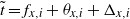
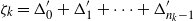
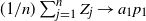
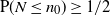
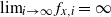
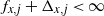
). Please see Figure 1 for the case when the duration of fire is always zero, and Figure 2 for the general case. Interestingly, the graphic representation of the process is somewhat reminiscent of direct percolation models, though we could not find a direct connection which would be useful in obtaining additional insights.
$\theta_{x-1,j}>0$
). Please see Figure 1 for the case when the duration of fire is always zero, and Figure 2 for the general case. Interestingly, the graphic representation of the process is somewhat reminiscent of direct percolation models, though we could not find a direct connection which would be useful in obtaining additional insights.
Graphical representation in the case
 $\theta\equiv 0$
, and a constant
$\theta\equiv 0$
, and a constant
 $\Delta\equiv a>0$
. Solid arrows represent the spread of fire, whereas dotted arrows indicate unsuccessful attempts to spread. The black dots mark the appearance of trees and green lines denote periods during which a tree occupies a site before it burns. The highlighted line of arrows represents the infinite fire.
$\Delta\equiv a>0$
. Solid arrows represent the spread of fire, whereas dotted arrows indicate unsuccessful attempts to spread. The black dots mark the appearance of trees and green lines denote periods during which a tree occupies a site before it burns. The highlighted line of arrows represents the infinite fire.

Graphical representation of the forest fire process for the general case. The black dots correspond to the appearance of trees; the green (red, respectively) segments are the periods when a site is occupied by a ‘healthy’ (burning, respectively) tree. The shaded areas represent the periods when a burning tree at site x affects site
 $x+1$
. The solid arrows show the fire spreading to a neighbouring tree; the dotted arrows represent the situations when the fire tried to spread unsuccessfully.
$x+1$
. The solid arrows show the fire spreading to a neighbouring tree; the dotted arrows represent the situations when the fire tried to spread unsuccessfully.

If the kth fire does not stop at x, and x started burning at time t, then we can draw an arrow from some point in the red segment with coordinates (x,s) with
 $s\in[t,t+\theta_{x,i})$
to the point
$s\in[t,t+\theta_{x,i})$
to the point
 $(x+1,s+\Delta_{x,i})$
such that the latter point is green, and each fire can be represented by a sequence of such arrows.
$(x+1,s+\Delta_{x,i})$
such that the latter point is green, and each fire can be represented by a sequence of such arrows.
Remark 1. As follows from the description of the model, distinct arrows from x to
 $x+1$
do not cross.
$x+1$
do not cross.
1.2. Structure of the paper
The rest of the paper is organized as follows. In Section 2 we prove the existence of the phenomenon called ‘the infinite fire’ in the case of non-trivial but identically distributed spreading times
 $\Delta$
. In Section 3 we consider the situation when the burning time
$\Delta$
. In Section 3 we consider the situation when the burning time
 $\theta$
is identically zero, yet the spreading time is either constant or asymptotically decreasing, and establish conditions for (non-)existence of an infinite fire. In Section 4, on the other hand, we show that if the spreading of the fire is immediate (
$\theta$
is identically zero, yet the spreading time is either constant or asymptotically decreasing, and establish conditions for (non-)existence of an infinite fire. In Section 4, on the other hand, we show that if the spreading of the fire is immediate (
 $\Delta=0$
) then no infinite fire occurs, and we also obtain some results on how quickly the fire spreads.
$\Delta=0$
) then no infinite fire occurs, and we also obtain some results on how quickly the fire spreads.
2. Existence of infinite fire
The infinite fire is a phenomenon which cannot happen in the forest fire models studied in either [Reference Comets, Menshikov and Volkov9] or [Reference Volkov15]; it arises, however, when there is a delay in the spreading of fire. Journal style requires that E and P should be roman for expectation and probability. Please check throughout.
Theorem 2.1. Suppose that
 $\mathrm{P}(\Delta>0)>0$
. Then almost surely (a.s.) there will be an infinite fire, i.e.
$\mathrm{P}(\Delta>0)>0$
. Then almost surely (a.s.) there will be an infinite fire, i.e.
 $\mathrm{P}(\inf\{k:\ n_k=\infty\}<\infty)=1$
.
$\mathrm{P}(\inf\{k:\ n_k=\infty\}<\infty)=1$
.
The next auxiliary statement is quite obvious, yet, for the sake of completeness, we present its short proof.
Lemma 2.1. Suppose that
 $\Delta$
is a non-negative random variable with
$\Delta$
is a non-negative random variable with
 $\mathrm{P}(\Delta>0)>0$
. Then for some constants
$\mathrm{P}(\Delta>0)>0$
. Then for some constants
 $\delta_1>0$
and
$\delta_1>0$
and
 $\delta_2>0$
 \begin{align*}\mathrm{P}\left(\sum_{j=1}^n \Delta_j'\ge n\delta_1\quad \text{for all }n\ge 1\right)\ge \delta_2,\end{align*}
where
 $\Delta_j'$
are i.i.d. copies of
$\Delta_j'$
are i.i.d. copies of
 $\Delta$
.
$\Delta$
.
Proof. By the condition of the lemma, there exist
 $a_1>0$
and
$a_1>0$
and
 $p_1>0$
such that
$p_1>0$
such that
 $\mathrm{P}(\Delta\ge a_1)$
 $\ge p_1$
. Hence,
$\ge p_1$
. Hence,
 $\Delta_j'$
is stochastically larger than
$\Delta_j'$
is stochastically larger than
 \begin{align*}Z_j=\begin{cases}a_1, &\text{with probability } p_1;\\0, &\text{with probability } 1-p_1\end{cases}\end{align*}
and we can assume that
 $Z_j$
are also i.i.d. Consequently, it suffices to show that
$Z_j$
are also i.i.d. Consequently, it suffices to show that
 \begin{align*}\mathrm{P}\Bigg(\sum_{j=1}^n Z_j\ge n\delta_1\text{ for all }n=1,2,\ldots\Bigg)\ge \delta_2\end{align*}
where
 $\delta_1\,:\!=\,\mathrm{E} Z_j/2=a_1p_1/2>0$
.
$\delta_1\,:\!=\,\mathrm{E} Z_j/2=a_1p_1/2>0$
.
By the strong law of large numbers
 $(1/n) \sum_{j=1}^n Z_j\to a_1p_1$
a.s. as
$(1/n) \sum_{j=1}^n Z_j\to a_1p_1$
a.s. as
 $n\to\infty$
, hence, since
$n\to\infty$
, hence, since
 $\delta_1<\mathrm{E} Z_J$
, a.s. there exists a (random)
$\delta_1<\mathrm{E} Z_J$
, a.s. there exists a (random)
 $N=N(\omega)$
such that
$N=N(\omega)$
such that
 $\sum_{j=1}^n Z_j\ge n\delta_1$
for all
$\sum_{j=1}^n Z_j\ge n\delta_1$
for all
 $n \ge N$
. Since N is finite, for some non-random
$n \ge N$
. Since N is finite, for some non-random
 $n_0\ge 1$
we have
$n_0\ge 1$
we have
 $\mathrm{P}(N\le n_0)\ge 1/2$
. As
$\mathrm{P}(N\le n_0)\ge 1/2$
. As
 $Z_j\in\{0,a_1\}$
, we have
$Z_j\in\{0,a_1\}$
, we have
 \begin{align*}\frac12&\le \mathrm{P}\Bigg( \sum_{j=1}^n Z_j\ge n\delta_1\ \forall n\gt n_0\Bigg)\le\mathrm{P}\Bigg( \sum_{j=1}^n Z_j\ge n\delta_1\ \forall n \gt n_0\mid Z_1=\ldots=Z_{n_0}=a_1\Bigg)\\[2pt] & =\frac{\mathrm{P}\left( \sum_{j=1}^n Z_j\ge n\delta_1\ \forall n \gt n_0\text{ and } Z_1=Z_2=\ldots=Z_{n_0}=a_1\right)}{\mathrm{P}\left( Z_1=Z_2=\ldots=Z_{n_0}=a_1\right)}\end{align*}
 \begin{align*}& =\frac{\mathrm{P}\left( \sum_{j=1}^n Z_j\ge n\delta_1\ \forall n\ge 1\text{ and } Z_1=Z_2=\ldots=Z_{n_0}=a_1\right)}{p_1^{n_0}}\\ & \le \frac{\mathrm{P}\left( \sum_{j=1}^n Z_j\ge n\delta_1\ \forall n\ge 1\right)}{p_1^{n_0}}\end{align*}
so the Lemma holds with e.g.
 $\delta_2\,:\!=\,p_1^{n_0}/2>0$
.
$\delta_2\,:\!=\,p_1^{n_0}/2>0$
.
Proof of Theorem
2.1. First, we show that for any
 $x\in \mathbb{Z}_+$
the fire will eventually reach x. In fact, by induction we show a stronger statement: for each
$x\in \mathbb{Z}_+$
the fire will eventually reach x. In fact, by induction we show a stronger statement: for each
 $x=0,1,2,\ldots$
there will be infinitely many fires that reach the site x and they will occur at arbitrary large times (i.e. all
$x=0,1,2,\ldots$
there will be infinitely many fires that reach the site x and they will occur at arbitrary large times (i.e. all
 $f_{x,i}$
are finite, and
$f_{x,i}$
are finite, and
 $f_{x,i}\nearrow\infty$
as i increases). The proof is based on induction.
$f_{x,i}\nearrow\infty$
as i increases). The proof is based on induction.
For site
 $x=0$
this fact is trivial as
$x=0$
this fact is trivial as
 $f_{0,k}\equiv \nu_k$
, see (1). Now suppose that our statement is true for some
$f_{0,k}\equiv \nu_k$
, see (1). Now suppose that our statement is true for some
 $x\geq 0$
. This means that there are infinitely many fires that start at times
$x\geq 0$
. This means that there are infinitely many fires that start at times
 $f_{x,1} \lt f_{x,2} \lt \ldots$
. Since the probability of not having a single tree at
$f_{x,1} \lt f_{x,2} \lt \ldots$
. Since the probability of not having a single tree at
 $x+1$
by time s is
$x+1$
by time s is
 $\mathrm{e}^{-s}\downarrow 0$
and
$\mathrm{e}^{-s}\downarrow 0$
and
 $\lim_{i\to\infty}f_{x,i}=\infty$
, eventually for some time
$\lim_{i\to\infty}f_{x,i}=\infty$
, eventually for some time
 $f_{x,j}$
there will be a tree at
$f_{x,j}$
there will be a tree at
 $x+1$
so it will start burning at time
$x+1$
so it will start burning at time
 $f_{x,j}+\Delta_{x,j}<\infty$
and burn during time
$f_{x,j}+\Delta_{x,j}<\infty$
and burn during time
 $\theta_{x+1,1}\ge 0$
; thus, we ensured that there will be at least one fire at
$\theta_{x+1,1}\ge 0$
; thus, we ensured that there will be at least one fire at
 $x+1$
. Now consider the process after the time
$x+1$
. Now consider the process after the time
 $f_{x,j}+\Delta_{x,j}+\theta_{x+1,1}$
. It takes an exponentially distributed time for a new tree to appear at
$f_{x,j}+\Delta_{x,j}+\theta_{x+1,1}$
. It takes an exponentially distributed time for a new tree to appear at
 $x+1$
; after that, it will eventually be burnt by a fire started at site x at some time
$x+1$
; after that, it will eventually be burnt by a fire started at site x at some time
 $f_{x,j'}$
with
$f_{x,j'}$
with
 $j'>j$
. This fire will start burning the tree at
$j'>j$
. This fire will start burning the tree at
 $x+1$
again at time
$x+1$
again at time
 $f_{x,j'}+\Delta_{x,j'}$
. Similar arguments hold for the third fire, the fourth fire, etc. The exponential waiting time for the appearance of new trees also implies that
$f_{x,j'}+\Delta_{x,j'}$
. Similar arguments hold for the third fire, the fourth fire, etc. The exponential waiting time for the appearance of new trees also implies that
 $f_{x+1,j}$
is stochastically larger than the time of arrival of the jth point of a Poisson process with rate 1, yielding
$f_{x+1,j}$
is stochastically larger than the time of arrival of the jth point of a Poisson process with rate 1, yielding
 $f_{x+1,i}\to\infty$
. The induction step is finished.
$f_{x+1,i}\to\infty$
. The induction step is finished.
Let
 $m_1$
denote the location of the tree, farthest from the origin, burnt by the first fire; if the fire continues indefinitely, we let
$m_1$
denote the location of the tree, farthest from the origin, burnt by the first fire; if the fire continues indefinitely, we let
 $m_1=+\infty$
. For
$m_1=+\infty$
. For
 $k\ge 2$
, we recursively define
$k\ge 2$
, we recursively define
 $m_k$
as the location of the tree, farthest from the origin, burnt by the first fire which reaches beyond
$m_k$
as the location of the tree, farthest from the origin, burnt by the first fire which reaches beyond
 $m_{k-1}$
; we can think of
$m_{k-1}$
; we can think of
 $m_k$
as the successive maxima reached by the fires. If
$m_k$
as the successive maxima reached by the fires. If
 $m_{k-1}=\infty$
for some k, we set
$m_{k-1}=\infty$
for some k, we set
 $m_{k}=m_{k+1}=\ldots=\infty$
as well. The successive maxima obviously satisfy
$m_{k}=m_{k+1}=\ldots=\infty$
as well. The successive maxima obviously satisfy
 $0\le m_1 \lt m_2\lt m_3\lt\ldots$
(with the convention
$0\le m_1 \lt m_2\lt m_3\lt\ldots$
(with the convention
 $\infty<\infty$
).
$\infty<\infty$
).
Let
 $A_k=\{m_k<\infty\}$
, i.e. the kth fire was finite, and let
$A_k=\{m_k<\infty\}$
, i.e. the kth fire was finite, and let
 $T_k=f_{m_k,1}+\theta_{m_k,1}$
be the time when the site
$T_k=f_{m_k,1}+\theta_{m_k,1}$
be the time when the site
 $m_k$
stops burning for the first time. Let
$m_k$
stops burning for the first time. Let
 $\mathcal{F}_k$
be the
$\mathcal{F}_k$
be the
 $\sigma$
-algebra (note that this is a sigma-algebra generated by the stopping time rather than a discrete time) generated by the states of sites
$\sigma$
-algebra (note that this is a sigma-algebra generated by the stopping time rather than a discrete time) generated by the states of sites
 $\{0,1,\ldots,m_k+1\}$
during the period
$\{0,1,\ldots,m_k+1\}$
during the period
 $[0,T_k]$
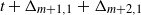
; we do not include in it any events related to appearances of the trees at sites
$[0,T_k]$
; we do not include in it any events related to appearances of the trees at sites
 $m_k+2,m_k+3,\ldots$
. We want to compute a lower bound on
$m_k+2,m_k+3,\ldots$
. We want to compute a lower bound on
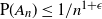
 $\mathrm{P}(A_{k+1}^c\mid \mathcal{F}_{k})$
, assuming that
$\mathrm{P}(A_{k+1}^c\mid \mathcal{F}_{k})$
, assuming that
 $A_k$
has occurred and
$A_k$
has occurred and
 $m_k=m$
. Suppose that the fire has reached
$m_k=m$
. Suppose that the fire has reached
 $m+1$
by some time t (note that
$m+1$
by some time t (note that
 $t>T_k$
). It takes
$t>T_k$
). It takes
 $\Delta_{m+1,1}$
units of time for the fire to reach
$\Delta_{m+1,1}$
units of time for the fire to reach
 $m+2$
. Assuming that there is a tree at
$m+2$
. Assuming that there is a tree at
 $m+2$
by that time (i.e.
$m+2$
by that time (i.e.
 $t+\Delta_{m+1,1}$
), the fire will continue to
$t+\Delta_{m+1,1}$
), the fire will continue to
 $m+3$
if there is a tree at
$m+3$
if there is a tree at
 $m+3$
by time
$m+3$
by time
 $t+\Delta_{m+1,1}+\Delta_{m+2,1}$
, and so on. Thus, the fire will continue ad infinitum, provided that
$t+\Delta_{m+1,1}+\Delta_{m+2,1}$
, and so on. Thus, the fire will continue ad infinitum, provided that
 \begin{align*}&\text{there is a tree at site $(m+i)$ by time }\ t+\Delta_{m+1,1}\\&\quad+ \Delta_{m+2,1}+\cdots+\Delta_{m+i-1,1}\quad \text{for each }i=2,3,\ldots\end{align*}
Since the probability that there is no tree at site x by time
 $s\ge 0$
is
$s\ge 0$
is
 $\mathrm{e}^{-s}$
(assuming no previous fires at x), the probability of the above event given t and
$\mathrm{e}^{-s}$
(assuming no previous fires at x), the probability of the above event given t and
 $\{\Delta_{m+i,1}\}_{i=1}^\infty$
is
$\{\Delta_{m+i,1}\}_{i=1}^\infty$
is
 \begin{align}\prod_{i=2}^\infty \left(1-\mathrm{e}^{-t-\sum_{k=1}^{i-1}\Delta_{m+k,1}}\right)\ge\prod_{i=2}^\infty \left(1-\mathrm{e}^{-\sum_{k=1}^{i-1}\Delta_{m+k,1}}\right).\end{align}
At the same time, by Lemma 2.1
 \begin{align*}\mathrm{P}\left(\mathrm{e}^{-\sum_{j=1}^n \Delta_j'}\le \mathrm{e}^{-n\delta_1}\text{ for all }n=1,2,\ldots\right)\ge \delta_2,\end{align*}
hence if we use the notation
 \begin{align*}\epsilon_0\,:\!=\,\prod_{n=1}^\infty \left(1-\mathrm{e}^{-n\delta_1}\right)>0\end{align*}
then the probability that the right-hand side of (2) is larger than
 $\epsilon_0$
is no less than
$\epsilon_0$
is no less than
 $\delta_2$
. As a result,
$\delta_2$
. As a result,
 \begin{align*}\mathrm{P}(A_{k+1}^c\mid\mathcal{F}_k)\ge \epsilon_0\delta_2>0\quad\text{ for all }k\ge 1\end{align*}
and, hence, by the conditional Borel–Cantelli lemma there will be an infinite fire a.s.
3. Instant burning
In this section, we consider the case when
 $\theta=0$
and
$\theta=0$
and
 $\mathrm{E}\Delta_x>0$
, that is, the trees are burnt instantly but the expected time for the fire to spread from site x to
$\mathrm{E}\Delta_x>0$
, that is, the trees are burnt instantly but the expected time for the fire to spread from site x to
 $x+1$
is strictly positive.
$x+1$
is strictly positive.
Theorem 3.1. Suppose
 $\theta\equiv 0$
,
$\theta\equiv 0$
,
 $0<\mathrm{E}\Delta<\infty$
, and
$0<\mathrm{E}\Delta<\infty$
, and
 $\mathrm{Var}(\Delta)>0$
. Then there is only one infinite fire.
$\mathrm{Var}(\Delta)>0$
. Then there is only one infinite fire.
Remark 3.1. The non-random case
 $\Delta\equiv \mathrm{const}>0$
will be covered later in Theorem 3.2.
$\Delta\equiv \mathrm{const}>0$
will be covered later in Theorem 3.2.
Proof. The existence of infinite fire follows from Theorem 2.1 since
 $\mathrm{E}\Delta>0$
implies
$\mathrm{E}\Delta>0$
implies
 $\mathrm{P}(\Delta>0)>0$
, so we only need to show that there cannot be a second infinite fire.
$\mathrm{P}(\Delta>0)>0$
, so we only need to show that there cannot be a second infinite fire.
For each site
 $x\in\mathbb{Z}_+$
let
$x\in\mathbb{Z}_+$
let
 $i_x$
be the index of the fire for this site, which turned out to be the first infinite fire (hence, there will be an
$i_x$
be the index of the fire for this site, which turned out to be the first infinite fire (hence, there will be an
 $x_1$
such that for all
$x_1$
such that for all
 $x>x_1$
we have
$x>x_1$
we have
 $i_x=1$
).
$i_x=1$
).
Assume now that there is a second infinite fire. Since for any
 $t>0$
the number of distinct fires at each site x by time t is a.s. finite, there will be a (random) site
$t>0$
the number of distinct fires at each site x by time t is a.s. finite, there will be a (random) site
 $x_2$
such that each site with
$x_2$
such that each site with
 $x>x_2$
was not burnt by any finite fire between the times when it was burnt by the first and the second infinite fire. Hence, for each
$x>x_2$
was not burnt by any finite fire between the times when it was burnt by the first and the second infinite fire. Hence, for each
 $x>x^*=\max(x_1,x_2)$
, the first (the second, respectively) fire to burn x is, in fact, the first (the second, respectively) infinite fire. Since burning is immediate (
$x>x^*=\max(x_1,x_2)$
, the first (the second, respectively) fire to burn x is, in fact, the first (the second, respectively) infinite fire. Since burning is immediate (
 $\theta\equiv 0$
), for
$\theta\equiv 0$
), for
 $x>x^*$
,
$x>x^*$
,
 \begin{align*} f_{x+1,1}=f_{x,1}+\Delta_{x,1}\quad\text{and}\quad f_{x+1,2}=f_{x,2}+\Delta_{x,2}.\end{align*}
Let us define
 $S_x=\sum_{k=1}^x\xi_k,$
where
$S_x=\sum_{k=1}^x\xi_k,$
where
 $\xi_k=\Delta_{k,2}-\Delta_{k,1}$
are i.i.d. mean-zero random variables. Then
$\xi_k=\Delta_{k,2}-\Delta_{k,1}$
are i.i.d. mean-zero random variables. Then
 $f_{x,i_x+1}-f_{x,i_x}=C(x^*)+S_x$
for
$f_{x,i_x+1}-f_{x,i_x}=C(x^*)+S_x$
for
 $x\ge x^*$
where
$x\ge x^*$
where
 $C(x^*)$
is some quantity depending on
$C(x^*)$
is some quantity depending on
 $x^*$
only. Indeed, for all sites at locations
$x^*$
only. Indeed, for all sites at locations
 $x>x^*$
, the first fire to burn x will be the first infinite fire, and the second fire to burn x will be the second infinite fire. Since
$x>x^*$
, the first fire to burn x will be the first infinite fire, and the second fire to burn x will be the second infinite fire. Since
 $S_x$
is a one-dimensional zero-mean random walk, it is recurrent by [Reference Spitzer14, P8, Section I.2] and hence
$S_x$
is a one-dimensional zero-mean random walk, it is recurrent by [Reference Spitzer14, P8, Section I.2] and hence
 $\mathrm{P}(\liminf_{x\to\infty} S_x=-\infty\mid x^*)=1$
, which contradicts the fact that we must always have
$\mathrm{P}(\liminf_{x\to\infty} S_x=-\infty\mid x^*)=1$
, which contradicts the fact that we must always have
 $f_{x,i_x+1}>f_{x,i_x}$
.
$f_{x,i_x+1}>f_{x,i_x}$
.
3.1. Constant spreading time
Recall that the burning time
 $\theta$
is assumed to be zero, and assume additionally that
$\theta$
is assumed to be zero, and assume additionally that
 $\Delta$
is the same non-random positive constant at all locations; in this section we want to study this special case. An interesting fact, observed by Edward Crane, is that after the infinite fire, the model here can be coupled with that of [Reference Volkov15]. We have already shown that there exists an infinite fire in this case; now we are interested in finding out the distribution of when exactly the infinite fire starts, and what the index
$\Delta$
is the same non-random positive constant at all locations; in this section we want to study this special case. An interesting fact, observed by Edward Crane, is that after the infinite fire, the model here can be coupled with that of [Reference Volkov15]. We have already shown that there exists an infinite fire in this case; now we are interested in finding out the distribution of when exactly the infinite fire starts, and what the index
 $\kappa$
of that fire can be.
$\kappa$
of that fire can be.
Theorem 3.2. Assume that
 $\theta\equiv 0$
and
$\theta\equiv 0$
and
 $\Delta\equiv a>0$
. Suppose that the infinite fire starts at site 0 at some time
$\Delta\equiv a>0$
. Suppose that the infinite fire starts at site 0 at some time
 $T\ge 0$
(which is, of course, random). Then this fire reaches point
$T\ge 0$
(which is, of course, random). Then this fire reaches point
 $x\ge 1$
precisely at time
$x\ge 1$
precisely at time
 $T+ax$
, and if we use the notation
$T+ax$
, and if we use the notation
 $\hat \eta_x(t)=\eta_x(t+T+ax)$
,
$\hat \eta_x(t)=\eta_x(t+T+ax)$
,
 $t\ge 0$
, then the process
$t\ge 0$
, then the process
 $\hat\eta$
is exactly that introduced in [Reference Volkov15], i.e. that with
$\hat\eta$
is exactly that introduced in [Reference Volkov15], i.e. that with
 $\theta=\Delta\equiv 0$
.
$\theta=\Delta\equiv 0$
.
Proof. This fact follows immediately from the definition of the process
 $\hat\eta_x(t)$
and can be also seen from the graphical representation of the fire process (see Figure 1), where all the arrows have the same slope a, and the infinite fire corresponds to a straight line going from (0,T) towards infinity at the constant slope a.
$\hat\eta_x(t)$
and can be also seen from the graphical representation of the fire process (see Figure 1), where all the arrows have the same slope a, and the infinite fire corresponds to a straight line going from (0,T) towards infinity at the constant slope a.
To get an estimate of when the infinite fire starts, observe the following. The times of consecutive fires at the origin form a Poisson process, and thus the kth fire starts at time
 $\nu_k=\xi_1+\xi_2+\cdots+\xi_k$
where
$\nu_k=\xi_1+\xi_2+\cdots+\xi_k$
where
 $\xi_i$
are i.i.d. exponential(1) random variables (see (1)). Let
$\xi_i$
are i.i.d. exponential(1) random variables (see (1)). Let
 $\kappa\ge 1$
be the index of the infinite fire, thus
$\kappa\ge 1$
be the index of the infinite fire, thus
 $T=\nu_\kappa$
. In the following statement we estimate the probability that the first fire is infinite.
$T=\nu_\kappa$
. In the following statement we estimate the probability that the first fire is infinite.
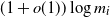
Proposition 3.1. We make the same assumptions as in Theorem 3.2. Then
 \begin{align*}1-\frac{1}{2\mu}\le \mathrm{P}(\kappa=1)\le \mu(1-\mathrm{e}^{-1/\mu}),\end{align*}
where
 $\mu\,:\!=\,\mathrm{e}^a-1$
. Hence, for large
$\mu\,:\!=\,\mathrm{e}^a-1$
. Hence, for large
 $a>0$
we have
$a>0$
we have
 $\mathrm{P}(\kappa=1)=1-1/{2(\mathrm{e}^a-1)}+o(1)$
.
$\mathrm{P}(\kappa=1)=1-1/{2(\mathrm{e}^a-1)}+o(1)$
.
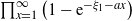
Proof. The first fire burns 0 at time
 $\xi_1$
. For this fire to spread indefinitely, one needs to have at least one tree at position x at time
$\xi_1$
. For this fire to spread indefinitely, one needs to have at least one tree at position x at time
 $\xi_1+ax$
for each
$\xi_1+ax$
for each
 $x\in\{1,2,\ldots\}$
; given
$x\in\{1,2,\ldots\}$
; given
 $\xi_1$
, this probability can be computed as
$\xi_1$
, this probability can be computed as
 $\prod_{x=1}^{\infty}\left(1-\mathrm{e}^{-\xi_1-ax}\right)$
.
$\prod_{x=1}^{\infty}\left(1-\mathrm{e}^{-\xi_1-ax}\right)$
.
Since for any sequence
 $y_1,y_2,\ldots\in[0,1]$
we have
$y_1,y_2,\ldots\in[0,1]$
we have
 \begin{align}1-\sum_{k=1}^\infty y_k \le \prod_{k=1}^\infty(1-y_k)\le \exp\left(-\sum_{k=1}^\infty y_k\right),\end{align}
and
 \begin{align*}\sum_{x=1}^\infty \mathrm{e}^{-\xi_1-ax}=\frac{\mathrm{e}^{-\xi_1}}{\mathrm{e}^a-1}.\end{align*}
By taking the expectation over
 $\xi_1$
, we get
$\xi_1$
, we get
 \begin{align*}\mathrm{P}(\kappa=1)&=\mathrm{E} \prod_{x=1}^{\infty}\left(1-\mathrm{e}^{-\xi_1-ax}\right)\le\int_0^\infty\exp\left(-\frac{\mathrm{e}^{-u}}{\mathrm{e}^a-1}\right) \mathrm{e}^{-u}\, \mathrm{d}u\\[5pt] &=\int_0^1\exp\left(-\frac{v}{\mathrm{e}^a-1}\right) \mathrm{d}v=(\mathrm{e}^a-1)\left(1-\mathrm{e}^{-\frac1{\mathrm{e}^a-1}}\right).\end{align*}
On the other hand, by (3)
 \begin{align*}\mathrm{P}(\kappa=1)&\ge\int_0^\infty\left(1-\frac{\mathrm{e}^{-u}}{\mathrm{e}^a-1}\right) \mathrm{e}^{-u}\,\mathrm{d}u=1-\frac1{2(\mathrm{e}^a-1)},\end{align*}
which completes the proof.
Remark 3.2. A much better approximation
 \begin{align*}\mathrm{P}(\kappa=1)\approx 1 - \frac{\mathrm{e}^{-a}+\mathrm{e}^{-2a}}2 - \frac{\mathrm{e}^{-3a}}6\end{align*}
can be obtained by using a tighter lower bound of
 $\prod_{k=1}^\infty (1-y_k)$
. It gives the relative error of
$\prod_{k=1}^\infty (1-y_k)$
. It gives the relative error of
 $0.01$
or less for
$0.01$
or less for
 $a\ge 1/2$
, and at most
$a\ge 1/2$
, and at most
 $0.07$
for
$0.07$
for
 $1/2\ge a\ge 1/3$
.
$1/2\ge a\ge 1/3$
.
Suppose the first fire did not become the infinite fire; let
 $m_1$
be the right-most point burnt by it. By arguments similar to those in Theorem 3.2, we can couple our process after time
$m_1$
be the right-most point burnt by it. By arguments similar to those in Theorem 3.2, we can couple our process after time
 $\nu_1$
with the simple fire process
$\nu_1$
with the simple fire process
 $\hat\eta_x(t)$
from [Reference Volkov15] such that
$\hat\eta_x(t)$
from [Reference Volkov15] such that
 \begin{align*}\hat\eta_x(t)=\eta_x(\nu_1+ax+t)\quad \text{for } x\in\{0,1,\ldots,m_1,m_1+1\}.\end{align*}
Let us also observe that given
 $\nu_1$
,
$\nu_1$
,
 \begin{align*}\mathrm{P}(m_1=k)=\mathrm{e}^{-\nu_1-a(k+1)}\prod_{x=1}^{k}\left(1-\mathrm{e}^{-\nu_1-ax}\right),\quad k=1,2,\ldots.\end{align*}
Let
 $\delta_1=1$
and, assuming that the first fire was not infinite, let
$\delta_1=1$
and, assuming that the first fire was not infinite, let
 $\delta_2$
be the index of the first fire which extends beyond
$\delta_2$
be the index of the first fire which extends beyond
 $m_1$
, i.e., burns site
$m_1$
, i.e., burns site
 $m_1+1$
. Denote by
$m_1+1$
. Denote by
 $m_2$
(
$m_2$
(
 $\ge m_1+1$
) the right-most point burnt by this fire. Then, given the time when it started, that is
$\ge m_1+1$
) the right-most point burnt by this fire. Then, given the time when it started, that is
 $\nu_{\delta_2}$
,
$\nu_{\delta_2}$
,
 \begin{align*}\mathrm{P}(m_2=m_1+k\mid \nu_{\delta_2})=\mathrm{e}^{-\nu_{\delta_2}-a(m_1+k+1)}\prod_{x=m_1+2}^{m_1+k}\left(1-\mathrm{e}^{-\nu_{\delta_2}-ax}\right),\quad k=1,2,3,\ldots.\end{align*}
Similarly, one can define pairs
 $(\delta_3,m_3)$
,
$(\delta_3,m_3)$
,
 $(\delta_4,m_4)$
, etc., until
$(\delta_4,m_4)$
, etc., until
 $(\delta_N,m_N)$
where
$(\delta_N,m_N)$
where
 $\delta_N=\kappa$
and
$\delta_N=\kappa$
and
 $m_N=+\infty$
.
$m_N=+\infty$
.
Now note that from coupling with the process in [Reference Volkov15], we have
 $\nu_{\delta_{k+1}}-\nu_{\delta_{k}}=\hat\tau_{m_k+1}$
where
$\nu_{\delta_{k+1}}-\nu_{\delta_{k}}=\hat\tau_{m_k+1}$
where
 $\hat\tau_z$
is the first time when the original forest fire process, that with
$\hat\tau_z$
is the first time when the original forest fire process, that with
 $\Delta=\theta=0$
, burns site
$\Delta=\theta=0$
, burns site
 $z\ge 1$
. Hence,
$z\ge 1$
. Hence,
 $\nu_{\delta_k}=\psi_k(m)$
, where
$\nu_{\delta_k}=\psi_k(m)$
, where
 \begin{align}\psi_k(\mu)=\sum_{\ell=0}^k\hat\tau_{\mu_\ell+1},\end{align}
where we set
 $\mu_0\,:\!=\,-1$
and, thus,
$\mu_0\,:\!=\,-1$
and, thus,
 $\hat\tau_0$
has the same
$\hat\tau_0$
has the same
 $\exp(1)$
distribution as
$\exp(1)$
distribution as
 $\nu_1$
. As a result, for any positive integer n and a sequence
$\nu_1$
. As a result, for any positive integer n and a sequence
 $0\equiv \mu_0<\mu_1<\mu_2<\cdots<\mu_{n-1}$
,
$0\equiv \mu_0<\mu_1<\mu_2<\cdots<\mu_{n-1}$
,
 \begin{align*} &\mathrm{P}(\kappa\ge n,m_1=\mu_1,m_2=\mu_2,\ldots,m_{n-1}=\mu_{n-1}) \\[5pt] & = \mathrm{E}\Bigg[ \prod_{i=1}^{n-1} \mathrm{e}^{-\nu_{\delta_i}-a(\mu_{i-1}+1)} \prod_{x=\mu_{i-1}+1}^{\mu_{i}} \left(1-\mathrm{e}^{-\nu_{\delta_i}-ax}\right) \Bigg] \\[5pt] & = \mathrm{E}\Bigg[ \prod_{i=1}^{n-1} \Bigg( \mathrm{e}^{-(\psi_{i-1}(\mu)+a(\mu_{i-1}+1))} \prod_{x=\mu_{i-1}+1}^{\mu_{i}} \big(1-\mathrm{e}^{-(\psi_{i-1}(\mu)+ax)}\big)\Bigg) \Bigg] \\[5pt] & = \mathrm{E}\Bigg[\Bigg( \prod_{i=1}^{n-1} \mathrm{e}^{-(\psi_{i-1}(\mu)+a(\mu_{i-1}+1))} \Bigg) \prod_{x=1}^{\mu_{n-1}} \big( 1-\mathrm{e}^{ -(ax+\psi_{\min\{k:\ x\le \mu_k\}}(\mu)) } \big) \Bigg]. \end{align*}
Thus,
 \begin{align*}\mathrm{P}(\kappa>n)=&\mathrm{E}\left[\sum_{\mu_1=1}^\infty\sum_{\mu_2=\mu_1+1}^\infty\cdots\sum_{\mu_{n-1}=\mu_{n-2}+1}^\infty\Bigg( \prod_{i=1}^{n-1} \mathrm{e}^{-(\psi_{i-1}(\mu)+a(\mu_{i-1}+1))} \Bigg) \right.\\ & \qquad \left. \times \prod_{x=1}^{\mu_{n-1}} \left( 1-\mathrm{e}^{ -(ax+\psi_{\min\{k:\ x\le \mu_k\}}(\mu)) } \right) \right],\end{align*}
which expresses the probability in terms of random variables
 $\hat\tau_x$
whose distribution can be obtained explicitly from [Reference Volkov15, Lemma 1.1], and then by using (4).
$\hat\tau_x$
whose distribution can be obtained explicitly from [Reference Volkov15, Lemma 1.1], and then by using (4).
3.2. Non-identically distributed
$\Delta$

In this section, we modify the model to allow
 $\Delta_x$
,
$\Delta_x$
,
 $x=0,1,2,\ldots$
, to have different distributions, which may depend on the location.
$x=0,1,2,\ldots$
, to have different distributions, which may depend on the location.
Theorem 3.3. Let
 $c\le 1$
. Assume that either:
$c\le 1$
. Assume that either:
-
(a)
$\Delta_x\le c/x$
for all large x; or -
(b) for some
$C>0$
we have
$|\Delta_x|\le C$
for all x,
$\sum_x Var(\Delta_x)<\infty$
, and
$\left|\sum_x[\mathrm{E}\Delta_x-{c}/x]\right|$
$<\infty$
.


Then the infinite fire does not occur a.s., i.e.
 $\mathrm{P}(n_k<\infty\text{ for all }k )=1$
.
$\mathrm{P}(n_k<\infty\text{ for all }k )=1$
.
Conversely, if
 $c>1$
, and either:
$c>1$
, and either:
-
(c)
$\Delta_x> c/x$
for all large x; or -
(d)
$\mathrm{E} \Delta_x=\frac {c+o(1)}x$
and
$\mathrm{P}\left(\lim_{x\to\infty}\, |\Delta_x|\sqrt{x}=0\right)=1$
.


Then the infinite fire occurs a.s.
Proof. Let
 $c\le 1$
. We will only consider case (b), as case (a) is similar (and easier). Suppose the fire reaches some site
$c\le 1$
. We will only consider case (b), as case (a) is similar (and easier). Suppose the fire reaches some site
 $x\ge 1$
for the first time at time
$x\ge 1$
for the first time at time
 $t_x$
. Conditioned on this time
$t_x$
. Conditioned on this time
 $t_x$
, the probability that this fire will continue indefinitely is
$t_x$
, the probability that this fire will continue indefinitely is
 \begin{align*}q_x\,:\!=\,\prod_{n=x+1}^\infty \left(1-\mathrm{e}^{-(t_x+\Delta_{x}+\Delta_{x+1}+\cdots+\Delta_{n-1})}\right)=\prod_{n=x+1}^\infty \left(1-\mathrm{e}^{-(t_x+S_{x,n})}\right)\end{align*}
as it takes
 $S_{x,n}\,:\!=\,\Delta_{x}+\Delta_{x+1}+\cdots+\Delta_{n-1}$
units of time for the fire to reach site n and we need to ensure that already there is a tree at this location. Let
$S_{x,n}\,:\!=\,\Delta_{x}+\Delta_{x+1}+\cdots+\Delta_{n-1}$
units of time for the fire to reach site n and we need to ensure that already there is a tree at this location. Let
 $\xi_x=\Delta_x-{c}/x$
. Then
$\xi_x=\Delta_x-{c}/x$
. Then
 $\sum_x \xi_x$
converges a.s. by Kolmogorov’s three-series theorem. We have
$\sum_x \xi_x$
converges a.s. by Kolmogorov’s three-series theorem. We have
 \begin{align*}S_{x,n}=\sum_{i=x}^{n-1}\left(\xi_i+\frac{c}i\right)=c\log\frac{n}{x}+o_x(1)+\sum_{i=x}^{n-1}\xi_i=c\log\frac{n}{x}+o_x(1),\end{align*}
where
 $o_x(1)\to 0$
a.s. as
$o_x(1)\to 0$
a.s. as
 $x\to\infty$
. As a result,
$x\to\infty$
. As a result,
 \begin{align*} \mathrm{e}^{-t_x-S_{x,n}}=\mathrm{e}^{-t_x-o_x(1)}\,\left(\frac{x}{n}\right)^c \end{align*}
which is not summable in
 $n\ge 1$
as
$n\ge 1$
as
 $c\le 1$
, yielding
$c\le 1$
, yielding
 $q_x=0$
.
$q_x=0$
.
Now assume
 $c>1$
. We consider only the harder case (d). Let
$c>1$
. We consider only the harder case (d). Let
 $\Delta_x^{(i)}$
be the (random) spread time from site x to site
$\Delta_x^{(i)}$
be the (random) spread time from site x to site
 $x+1$
, for the fire number
$x+1$
, for the fire number
 $i=1,2,\ldots$
started at the origin. Note that some of the
$i=1,2,\ldots$
started at the origin. Note that some of the
 $\Delta_x^{(i)}$
will be irrelevant for the understanding of the process: for example, if the first fire reaches only site 1, and the second fire reaches site 3, then
$\Delta_x^{(i)}$
will be irrelevant for the understanding of the process: for example, if the first fire reaches only site 1, and the second fire reaches site 3, then
 $\Delta_1^{(1)},\Delta_2^{(1)}$
will be irrelevant for the behaviour of the process, but
$\Delta_1^{(1)},\Delta_2^{(1)}$
will be irrelevant for the behaviour of the process, but
 $\Delta_1^{(2)},\Delta_2^{(2)}$
will be relevant.
$\Delta_1^{(2)},\Delta_2^{(2)}$
will be relevant.
Let
 $\zeta_n\in\{1,2,\ldots\}$
be the index of the fire that burns n for the very first time. Pick a small
$\zeta_n\in\{1,2,\ldots\}$
be the index of the fire that burns n for the very first time. Pick a small
 $\delta>0$
such that
$\delta>0$
such that
 $c-\delta>1$
, and let
$c-\delta>1$
, and let
 \begin{align*}D_{n,i}&\,:\!=\,\left\{\sum_{x=0}^{n-1} \Delta_x^{(i)} \lt (c-\delta)\log n\right\},\\A_n&\,:\!=\,\{\text{the 1st fire which reaches the} n\text{th tree does not spread to the} (n+1)\text{th tree}\}.\end{align*}
Note that in this notation
 $\left(D_{n,\zeta_n}\right)^c=\{$
the fire which reaches the nth tree for the first time takes more than
$\left(D_{n,\zeta_n}\right)^c=\{$
the fire which reaches the nth tree for the first time takes more than
 $(c-\delta)\log n$
units of time from its start
$(c-\delta)\log n$
units of time from its start
 $\}$
.
$\}$
.
We have
 $0\le \Delta_x\le C_x$
a.s., where
$0\le \Delta_x\le C_x$
a.s., where
 $C_x\le \delta/{\sqrt {2x}}$
for all large x, yielding
$C_x\le \delta/{\sqrt {2x}}$
for all large x, yielding
 \begin{align*}\sum_{x=1}^{n-1} C_x^2\le \delta^2\log n\end{align*}
for large n. Since, also,
 \begin{align*}\sum_{x=1}^n \mathrm{E}\Delta_x =(c+o(1))\log(n)\end{align*}
by Hoeffding’s inequality,
 \begin{align*}\mathrm{P}\left(D_{n,i}\right)\le \exp\left(-\frac{2\delta^2\log^2 n }{\delta^2\log n}\right)=\frac1{n^2}.\end{align*}
To prove the existence of an infinite fire, it suffices to show that
 $A_n$
happens only finitely often, a.s. We have
$A_n$
happens only finitely often, a.s. We have
 \begin{align}\begin{split} \mathrm{P}(A_n)&=\mathrm{P}(A_n\cap D_{n,\zeta_n}^c)+\mathrm{P}(A_n\cap D_{n,\zeta_n})\leq \mathrm{P}\left(A_n\mid D_{n,\zeta_n}^c\right)+\mathrm{P}\left(D_{n,\zeta_n}\right)\\&=\sum_{i=1}^\infty \left[\mathrm{P}\left(A_n\mid D_{n,i}^c,\zeta_n=i\right)+\mathrm{P}\left(D_{n,i}\mid \zeta_n=i\right)\right]\times \mathrm{P}(\zeta_n=i)\\&\leq\sum_{i=1}^\infty\left[\mathrm{P}(\text{no tree at $(n+1)$ up to time }(c-\delta)\log n)+\mathrm{P}(D_{n,i}\mid \zeta_n=i)\right]\times \mathrm{P}(\zeta_n=i)\\&=\frac{1}{n^{c-\delta}}+\sum_{i=1}^\infty\mathrm{P}\left(D_{n,i}\mid \zeta_n=i\right)\times\mathrm{P}(\zeta_n=i)\leq\frac{1}{n^{c-\delta}}+\frac{1}{n^2},\end{split}\end{align}
which holds as long as we can show that
 \begin{align}\mathrm{P}\left(D_{n,i}\mid \zeta_n=i\right) \leq \mathrm{P}\left(D_{n,i}\right).\end{align}
Let us show that this is indeed the case. Observe that
 $\{\zeta_n=i\}=X\cap Y$
, where
$\{\zeta_n=i\}=X\cap Y$
, where
 \begin{align*}X&\,:\!=\,\{\text{the first}\, i-1\, \text{fires do not reach site }n\},\\Y&\,:\!=\,\{\text{the}\, i\,\text{th fire reaches site }n\}.\end{align*}
Note also that X and
 $D_{n,i}$
are independent since the distributions of the first
$D_{n,i}$
are independent since the distributions of the first
 $(i-1)$
fires are not influenced by the
$(i-1)$
fires are not influenced by the
 $\{\Delta_0^{(i)},\Delta_1^{(i)},\ldots,\Delta_{n-1}^{(i)}\}$
, and
$\{\Delta_0^{(i)},\Delta_1^{(i)},\ldots,\Delta_{n-1}^{(i)}\}$
, and
 $\mathrm{P}(Y)\geq \mathrm{P}\left(Y\mid D_{n,i}\right)$
, since the probability of the ith fire reaching n increases whenever any of
$\mathrm{P}(Y)\geq \mathrm{P}\left(Y\mid D_{n,i}\right)$
, since the probability of the ith fire reaching n increases whenever any of
 $\Delta_x^{(i)}$
in the above set increases. As a result,
$\Delta_x^{(i)}$
in the above set increases. As a result,
 \begin{align*}\mathrm{P}\left(X\cap Y\mid D_{n,i}\right)&=\mathrm{P}\left(X\mid Y,D_{n,i}\right)\, \mathrm{P}\left(Y\mid D_{n,i}\right)=\mathrm{P}(X\mid Y)\, \mathrm{P}\left(Y\mid D_{n,i}\right)\\ &\leq \mathrm{P}(X\mid Y)\, \mathrm{P}(Y)=\mathrm{P}(X\cap Y),\end{align*}
which together with the Bayes formula
 \begin{align*}\mathrm{P}\left(D_{n,i}\mid \zeta_n=i\right)=\frac{\mathrm{P}\left(\zeta_n=i\mid D_{n,i}\right)\times \mathrm{P}\left(D_{n,i}\right)}{\mathrm{P}\left(\zeta_n=i\right)}\end{align*}
yields (6).
Finally, by (5), since
 $c-\delta>1$
, the probabilities
$c-\delta>1$
, the probabilities
 $\mathrm{P}(A_n)$
are summable over n, and by the Borel–Cantelli lemma,
$\mathrm{P}(A_n)$
are summable over n, and by the Borel–Cantelli lemma,
 $A_n$
occurs finitely often, a.s. As a result, there cannot be infinitely many successive maxima, implying that an infinite fire a.s. exists.
$A_n$
occurs finitely often, a.s. As a result, there cannot be infinitely many successive maxima, implying that an infinite fire a.s. exists.
4. Instant spread, non-zero burning times
Throughout this section we assume that
 $\Delta\equiv 0$
but
$\Delta\equiv 0$
but
 $\theta\ge 0$
.
$\theta\ge 0$
.
Theorem 4.1. Suppose that
 $\Delta\equiv 0$
. Then a.s. there are no infinite fires.
$\Delta\equiv 0$
. Then a.s. there are no infinite fires.
Proof. Recall that
 $f_{x,i}$
denotes the time when the site
$f_{x,i}$
denotes the time when the site
 $x\in\mathbb{Z}_+$
is burnt for the ith time. Then at time
$x\in\mathbb{Z}_+$
is burnt for the ith time. Then at time
 $t=f_{x,1}$
there may already be trees at sites
$t=f_{x,1}$
there may already be trees at sites
 $x+1,x+2,\ldots$
and the fire will spread to those sites immediately (as
$x+1,x+2,\ldots$
and the fire will spread to those sites immediately (as
 $\Delta=0$
); however, since the probability of not having a single tree during time s is
$\Delta=0$
); however, since the probability of not having a single tree during time s is
 $\mathrm{e}^{-t}$
and these events are independent for each site
$\mathrm{e}^{-t}$
and these events are independent for each site
 $y> x$
, with probability one there will be a site
$y> x$
, with probability one there will be a site
 $y\ge x+1$
such that there are no trees there; we let y be the leftmost such site. This means that
$y\ge x+1$
such that there are no trees there; we let y be the leftmost such site. This means that
 \begin{align*}f_{x,1}=f_{x+1,1}=\cdots=f_{y-1,1} \lt f_{y,1}.\end{align*}
For this fire still to reach y, there must be a tree ‘planted’ at y during the time interval
 $[t,t+\theta_{y-1,1}]$
. Conditionally on
$[t,t+\theta_{y-1,1}]$
. Conditionally on
 $\theta_{y-1,1}$
, this probability equals
$\theta_{y-1,1}$
, this probability equals
 $1-\mathrm{e}^{-\theta_{y-1,1}}$
, so every time the fire spreads immediately from some site x to
$1-\mathrm{e}^{-\theta_{y-1,1}}$
, so every time the fire spreads immediately from some site x to
 $y-1$
, with probability
$y-1$
, with probability
 $p_*\,:\!=\,\mathrm{E} \mathrm{e}^{-\theta}>0$
, independently of the past, it will not spread further. Since this probability does not depend on x or s either, it means that a.s. the fire will eventually stop.
$p_*\,:\!=\,\mathrm{E} \mathrm{e}^{-\theta}>0$
, independently of the past, it will not spread further. Since this probability does not depend on x or s either, it means that a.s. the fire will eventually stop.
Now we want to study some further properties of the fire process. Recall that
 $m_k$
denotes the location of the tree, farthest from the origin, burnt by the kth fire.
$m_k$
denotes the location of the tree, farthest from the origin, burnt by the kth fire.
Lemma 4.1. Assume
 $\Delta\equiv 0$
and fix some
$\Delta\equiv 0$
and fix some
 $\epsilon\gt 0$
. The time
$\epsilon\gt 0$
. The time
 $f_{m_i,1}$
when the fire reaches
$f_{m_i,1}$
when the fire reaches
 $m_i$
for the first time is less than
$m_i$
for the first time is less than
 $(1+\epsilon)\log m_i$
for all but finitely many i, a.s.
$(1+\epsilon)\log m_i$
for all but finitely many i, a.s.
Proof. Suppose that the fire reaches site n at time
 $t=f_{n,1}$
. The probability that there is no tree at
$t=f_{n,1}$
. The probability that there is no tree at
 $n+1$
at this time is
$n+1$
at this time is
 $\mathrm{e}^{-t}$
, so in case
$\mathrm{e}^{-t}$
, so in case
 $t\ge (1+\epsilon)\log n$
, the probability of not spreading the fire further is less than
$t\ge (1+\epsilon)\log n$
, the probability of not spreading the fire further is less than
 \begin{align*}\mathrm{e}^{-(1+\epsilon)\log n}=\frac1{n^{1+\epsilon}}.\end{align*}
Hence,
 $\mathrm{P}(A_n)\le 1/{n^{1+\epsilon}}$
, where
$\mathrm{P}(A_n)\le 1/{n^{1+\epsilon}}$
, where
 \begin{align*}A_n=\{n\text{ is a local maximum and }f_{n,1}>(1+\epsilon)\log n)\},\end{align*}
so by the Borel–Cantelli lemma,
 $A_n$
occurs only for finitely many n a.s. From this, the statement follows.
$A_n$
occurs only for finitely many n a.s. From this, the statement follows.
The next statement is similar to [Reference Comets, Menshikov and Volkov9, Proposition 2].
Lemma 4.2. Assume
 $\Delta\equiv 0$
and fix some
$\Delta\equiv 0$
and fix some
 $\epsilon\gt 0$
. Let
$\epsilon\gt 0$
. Let
 \begin{align*}F_n=F_n(\epsilon)=\{\,f_{n,1}\ge (1-\epsilon)\log n\}.\end{align*}
Then
 \begin{align*}\mathrm{P}\left(F_n^c\right)<\mathrm{e}^{-n^\epsilon}\end{align*}
and, hence, the event
 $F_n^c$
a.s. occurs only finitely often.
$F_n^c$
a.s. occurs only finitely often.
Proof. In order to reach n by time t, there should be a tree at each location
 $x\in [0,n]$
by that time (or even earlier, because
$x\in [0,n]$
by that time (or even earlier, because
 $\theta>0$
), so
$\theta>0$
), so
 \begin{align*}\mathrm{P}(\,f_{n,1}<(1-\epsilon)\log n)\le \left(1-\mathrm{e}^{(1-\epsilon)\log n}\right)^{n}=\left[\left(1-\frac1{n^{1-\epsilon}}\right)^{n^{1-\epsilon}}\right]^{n^\epsilon}<\mathrm{e}^{-n^\epsilon}.\end{align*}
The second statement follows from the Borel–Cantelli lemma.
Lemmas 4.1 and 4.2 give a tight bound on
 $f_{m_i,1}$
, since by Lemma 4.2, that
$f_{m_i,1}$
, since by Lemma 4.2, that
 $f_{m_i,1}<(1-\epsilon)$
 $\log m_i$
, only finitely often a.s.
$\log m_i$
, only finitely often a.s.
Recall that
 $f_{x,2}$
is the time when the site x is burnt for the second time. We believe that the following holds, even though we cannot prove it.
$f_{x,2}$
is the time when the site x is burnt for the second time. We believe that the following holds, even though we cannot prove it.
Conjecture 4.1. There is a
 $c\ge 1$
, such that a.s. there exists a (possibly random)
$c\ge 1$
, such that a.s. there exists a (possibly random)
 $\kappa$
such
$\kappa$
such
 \begin{align}f_{m_i,2}\le c\log m_i\quad \text{for all }i\ge \kappa.\end{align}
The motivation for this conjecture is as follows. First of all, we already know that
 $(1-\epsilon)\log m_i<f_{m_i,1}<(1+\epsilon)\log m_i$
, for all large i a.s., regardless of the value of
$(1-\epsilon)\log m_i<f_{m_i,1}<(1+\epsilon)\log m_i$
, for all large i a.s., regardless of the value of
 $\theta$
. In the case where
$\theta$
. In the case where
 $\theta\equiv0$
, the difference
$\theta\equiv0$
, the difference
 $f_{m_i,2}-f_{m_i,1}$
has the same distribution as
$f_{m_i,2}-f_{m_i,1}$
has the same distribution as
 $f_{m_i,1}$
. Since altering
$f_{m_i,1}$
. Since altering
 $\theta$
does not have any effect on the order of
$\theta$
does not have any effect on the order of
 $f_{m_i}$
, we suspect it does not have any substantial effect on
$f_{m_i}$
, we suspect it does not have any substantial effect on
 $f_{m_i,2}-f_{m_i,1}$
either. Later, we show that the number of ‘jumps’ (continuous stretches of fire, please see the proof of part (b) of Lemma 4.3 for the exact definition) in the fire reaching
$f_{m_i,2}-f_{m_i,1}$
either. Later, we show that the number of ‘jumps’ (continuous stretches of fire, please see the proof of part (b) of Lemma 4.3 for the exact definition) in the fire reaching
 $m_i$
for the first time is of order
$m_i$
for the first time is of order
 $\log i$
, which is quite low compared with the order of
$\log i$
, which is quite low compared with the order of
 $m_i$
that exceeds
$m_i$
that exceeds
 $\exp\{\mathrm{e}^{\alpha i}\}$
, as we show later. This indicates that the path (using the graphic representation language) of the first fire reaching
$\exp\{\mathrm{e}^{\alpha i}\}$
, as we show later. This indicates that the path (using the graphic representation language) of the first fire reaching
 $m_i$
is not ‘very bumpy’, and thus it might behave more like a flat path (instantaneous burn). Hence, while we do not claim
$m_i$
is not ‘very bumpy’, and thus it might behave more like a flat path (instantaneous burn). Hence, while we do not claim
 $f_{m_i,2}-f_{m_i,1}$
equals
$f_{m_i,2}-f_{m_i,1}$
equals
 $(1+o(1))\log m_i$
, we have a strong reason to believe that it is at least of order
$(1+o(1))\log m_i$
, we have a strong reason to believe that it is at least of order
 $\log m_i$
.
$\log m_i$
.
Theorem 4.2. Suppose that
 $\Delta=0$
and
$\Delta=0$
and
 $\theta>0$
is constant. Assume that Conjecture 4.1 is true. Then
$\theta>0$
is constant. Assume that Conjecture 4.1 is true. Then
 $f_{n,1} = \mathcal{O}(\log n)$
, i.e. there exists a non-random
$f_{n,1} = \mathcal{O}(\log n)$
, i.e. there exists a non-random
 $M>0$
such that
$M>0$
such that
 $f_{n,1}\leq M\, \log n$
for large n.
$f_{n,1}\leq M\, \log n$
for large n.
We start with an auxiliary statement.
Lemma 4.3. Suppose that
 $\Delta=0$
and
$\Delta=0$
and
 $\theta>0$
is constant.
$\theta>0$
is constant.


Proof. (a) The statement is trivial for
 $r\le 1$
, since
$r\le 1$
, since
 $m_i\ge i$
, so from now on assume that
$m_i\ge i$
, so from now on assume that
 $r>1$
. Let
$r>1$
. Let
 $0 \lt \epsilon \lt 1/r$
. Suppose that the fire has reached
$0 \lt \epsilon \lt 1/r$
. Suppose that the fire has reached
 $m_i$
at time
$m_i$
at time
 $t\,:\!=\,f_{m_i,1}$
; without loss of generality, we can assume that t is sufficiently large.
$t\,:\!=\,f_{m_i,1}$
; without loss of generality, we can assume that t is sufficiently large.
Since the fire has successfully spread from
 $m_i-1$
to
$m_i-1$
to
 $m_i$
, this fire had reached
$m_i$
, this fire had reached
 $m_i-1$
at time
$m_i-1$
at time
 $t'\in( t-\theta,t]$
, and thus with probability at least
$t'\in( t-\theta,t]$
, and thus with probability at least
 $\mathrm{e}^{-2\theta}$
there will be no new tree at
$\mathrm{e}^{-2\theta}$
there will be no new tree at
 $m_i-1$
during the time interval
$m_i-1$
during the time interval
 $[t'+\theta,t+2\theta]$
(as
$[t'+\theta,t+2\theta]$
(as
 $t'+\theta$
is the time when the tree at
$t'+\theta$
is the time when the tree at
 $m_i-1$
stops burning). Under this event, the second fire to reach
$m_i-1$
stops burning). Under this event, the second fire to reach
 $m_i$
cannot happen before time
$m_i$
cannot happen before time
 $t+2\theta$
, which, in turn, provides the site
$t+2\theta$
, which, in turn, provides the site
 $m_i+1$
with at least
$m_i+1$
with at least
 $\theta$
units of time to grow a tree (there was none during the time
$\theta$
units of time to grow a tree (there was none during the time
 $[t,t+\theta]$
since we know that
$[t,t+\theta]$
since we know that
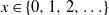
 $m_i$
was the local maximum by that time); please see Figure 3. Hence, with probability at least
$m_i$
was the local maximum by that time); please see Figure 3. Hence, with probability at least
 \begin{align}\mathrm{e}^{-2\theta}\cdot \left(1-\mathrm{e}^{-\theta}\right),\end{align}
 $f_{m_i+1,1}\in[\,f_{m_i,2}, f_{m_i,2}+\theta)$
, i.e. the second fire to reach
$f_{m_i+1,1}\in[\,f_{m_i,2}, f_{m_i,2}+\theta)$
, i.e. the second fire to reach
 $m_i$
will also reach
$m_i$
will also reach
 $m_i+1$
. However, by that time, there can already be the whole stretch of trees at sites
$m_i+1$
. However, by that time, there can already be the whole stretch of trees at sites
 $m_i+2,m_i+3,\ldots$
; in fact, the number
$m_i+2,m_i+3,\ldots$
; in fact, the number
 $L_i$
of consecutive sites which do have a tree by this time has a geometric distribution with parameter
$L_i$
of consecutive sites which do have a tree by this time has a geometric distribution with parameter
 $p=\mathrm{e}^{-f_{m_i+1,1}}<\mathrm{e}^{-t}$
. Let
$p=\mathrm{e}^{-f_{m_i+1,1}}<\mathrm{e}^{-t}$
. Let
 $\tilde{\mathcal{G}}^*$
be the sigma-algebra containing all the events which happened by time
$\tilde{\mathcal{G}}^*$
be the sigma-algebra containing all the events which happened by time
 $f_{m_i+1,1}$
to the left of
$f_{m_i+1,1}$
to the left of
 $m_i+1$
. Then
$m_i+1$
. Then
 \begin{align}\mathrm{P}\left(L_i\ge \frac 1p\mid \mathcal{G}^*\right)=\left(1-p\right)^{\lceil 1/p\rceil}=\mathrm{e}^{-1}+o(1),\end{align}
where
 $o(1)\to 0$
as
$o(1)\to 0$
as
 $p\to 0$
(i.e.
$p\to 0$
(i.e.
 $t\to \infty$
). Let
$t\to \infty$
). Let
 \begin{align}B_i\,:\!=\,\left\{m_{i+1}\ge m_i+m_i^{1-\epsilon}\right\}=\{L_i\geq m_i^{1-\epsilon}\}.\end{align}
If event
 $F_{m_i}$
from Lemma 4.2 occurs, then
$F_{m_i}$
from Lemma 4.2 occurs, then
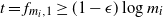 $t=f_{m_i,1}\ge (1-\epsilon)\log m_i$
yielding
$t=f_{m_i,1}\ge (1-\epsilon)\log m_i$
yielding
 $1/p> m_i^{1-\epsilon}$
. Taking into account the bound of probability (8) and (9), we obtain that
$1/p> m_i^{1-\epsilon}$
. Taking into account the bound of probability (8) and (9), we obtain that
 \begin{align}\mathrm{P}(B_i\mid \mathcal{G}^*)\ge \left[ \mathrm{e}^{-2\theta-1}\cdot \left(1-\mathrm{e}^{-\theta}\right)+o(1)\right] \times 1_{F_{m_i}}\ge c'\times 1_{F_{m_i}}\end{align}
for some
 $c'>0$
.
$c'>0$
.
How the second fire reaching
 $m_i$
can spread very far.
$m_i$
can spread very far.

Let
 $\mu_i=m_i^\epsilon$
. From Taylor expansion, we obtain that on
$\mu_i=m_i^\epsilon$
. From Taylor expansion, we obtain that on
 $B_i$
we have
$B_i$
we have
 \begin{align*}\mu_{i+1}-\mu_i\ge \epsilon+O(m_i^{-\epsilon})\ge \epsilon/2\end{align*}
for sufficiently large i; also, trivially,
 $\mu_{i+1}\ge \mu_i$
. Consequently, we can create a sequence of i.i.d. Bernoulli(c’) random variables
$\mu_{i+1}\ge \mu_i$
. Consequently, we can create a sequence of i.i.d. Bernoulli(c’) random variables
 $\xi_i$
,
$\xi_i$
,
 $i=1,2,\ldots$
, such that
$i=1,2,\ldots$
, such that
 $\mu_{i+1}-\mu_i$
is stochastically larger than
$\mu_{i+1}-\mu_i$
is stochastically larger than
 $({\epsilon}/2) \xi_i 1_{F_{m_i}}$
. By the strong law,
$({\epsilon}/2) \xi_i 1_{F_{m_i}}$
. By the strong law,
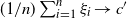 $(1/n)\sum_{i=1}^n\xi_i\to c'$
a.s., and at the same time
$(1/n)\sum_{i=1}^n\xi_i\to c'$
a.s., and at the same time
 \begin{align*}0\le \frac1n\sum_{i=1}^n\xi_i-\frac1n\sum_{i=1}^n\xi_i\, 1_{F_{m_i}}\le \frac{|\{i:\ F_{m_i}\text{ did not occur}\}|}n.\end{align*}
By Lemma 4.2, the quantity in the numerator is a.s. finite and does not depend on n, hence
 \begin{align*}\lim_{n\to\infty} \frac1n\sum_{i=1}^n\xi_i\, 1_{F_{m_i}}=c'\quad\text{a.s.}\end{align*}
This, in turn, leads to
 \begin{align*}\liminf_{i\to\infty} \frac{\mu_i}i\ge \frac{c'\,\epsilon}2\qquad \text{a.s.},\end{align*}
yielding
 \begin{align*}m_i\ge \left(\frac{c' \epsilon}3 i\right)^{1/\epsilon}\ge i^r\qquad\text{a.s.}\end{align*}
for all sufficiently large i, since
 $1/\epsilon\gt r$
.
$1/\epsilon\gt r$
.
(b) Consider the first fire that reaches beyond
 $m_i$
(the one which occurred at time
$m_i$
(the one which occurred at time
 $f_{m_i+1,1}$
). This fire will extend further to the right in several so-called ‘jumps’, rigorously defined in the next two paragraphs, until it eventually stops somewhere. The number of these jumps will be denoted by
$f_{m_i+1,1}$
). This fire will extend further to the right in several so-called ‘jumps’, rigorously defined in the next two paragraphs, until it eventually stops somewhere. The number of these jumps will be denoted by
 $N_i\in\{1,2,\ldots\}$
.
$N_i\in\{1,2,\ldots\}$
.
Let
 $L_{i,1}$
be the length of the maximum stretch of sites to the right of
$L_{i,1}$
be the length of the maximum stretch of sites to the right of
 $m_i$
burned at the same time as
$m_i$
burned at the same time as
 $m_i+1$
, so that
$m_i+1$
, so that
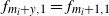 $f_{m_i+y,1}=f_{m_i+1,1}$
for
$f_{m_i+y,1}=f_{m_i+1,1}$
for
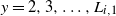 $y=2,3,\ldots,L_{i,1}$
. After the fire reaches site
$y=2,3,\ldots,L_{i,1}$
. After the fire reaches site
 $m_i+L_{i,1}$
, and
$m_i+L_{i,1}$
, and
 $m_i+L_{i,1}+1$
is empty at that time (since we know that the fire did not immediately go further), there are two possibilities: either with probability
$m_i+L_{i,1}+1$
is empty at that time (since we know that the fire did not immediately go further), there are two possibilities: either with probability
 $\mathrm{e}^{-\theta}$
within the next
$\mathrm{e}^{-\theta}$
within the next
 $\theta$
units of time no tree appears at the site
$\theta$
units of time no tree appears at the site
 $m_i+L_{i,1}+1$
, or such a tree does appear.
$m_i+L_{i,1}+1$
, or such a tree does appear.
In the first case, we set
 $N_i=1$
and stop. In the latter case, we say that the fire has a jump at position
$N_i=1$
and stop. In the latter case, we say that the fire has a jump at position
 $m_i+L_{i,1}+1$
, meaning that the fire, whilst burning both
$m_i+L_{i,1}+1$
, meaning that the fire, whilst burning both
 $m_i+L_{i,1}$
and
$m_i+L_{i,1}$
and
 $m_i+L_{i,1}+1$
, reached the latter site with a delay (up to
$m_i+L_{i,1}+1$
, reached the latter site with a delay (up to
 $\theta$
;
$\theta$
;
 $0 \lt f_{m_i+L_{i,1}+1,1}-f_{m_i+L_{i,1},1} \lt \theta$
). In case of such a jump, the fire will immediately spread to the additional
$0 \lt f_{m_i+L_{i,1}+1,1}-f_{m_i+L_{i,1},1} \lt \theta$
). In case of such a jump, the fire will immediately spread to the additional
 $L_{i,2}$
sites to the right of
$L_{i,2}$
sites to the right of
 $m_i+L_{i,1}$
, and thus
$m_i+L_{i,1}$
, and thus
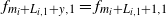 $f_{m_i+L_{i,1}+y,1}=f_{m_i+L_{i,1}+1,1}$
for
$f_{m_i+L_{i,1}+y,1}=f_{m_i+L_{i,1}+1,1}$
for
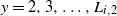 $y=2,3,\ldots,L_{i,2}$
, but there is no tree at the site
$y=2,3,\ldots,L_{i,2}$
, but there is no tree at the site
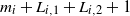 $m_i+L_{i,1}+L_{i,2}+1$
at this time.
$m_i+L_{i,1}+L_{i,2}+1$
at this time.
Similarly, we can define
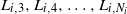 $L_{i,3},L_{i,4},\ldots,L_{i,N_i}$
, where
$L_{i,3},L_{i,4},\ldots,L_{i,N_i}$
, where
 $N_i$
is the number of continuous stretches of sites that were burnt at the same time (before the fire eventually stopped completely);
$N_i$
is the number of continuous stretches of sites that were burnt at the same time (before the fire eventually stopped completely);
 $N_i$
is the number of such jumps. As a result,
$N_i$
is the number of such jumps. As a result,
 $N_i$
is a geometric random variable with rate
$N_i$
is a geometric random variable with rate
 $\mathrm{e}^{-\theta}$
, and the site
$\mathrm{e}^{-\theta}$
, and the site
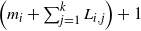 $\left(m_i+\sum_{j=1}^k L_{i,j}\right)+1$
is burnt slightly later than the site
$\left(m_i+\sum_{j=1}^k L_{i,j}\right)+1$
is burnt slightly later than the site
 $m_i+\sum_{j=1}^k L_{i,j}$
for each
$m_i+\sum_{j=1}^k L_{i,j}$
for each
 $k=1,2,\ldots,N_i-1$
, with the delay of up to
$k=1,2,\ldots,N_i-1$
, with the delay of up to
 $\theta$
.
$\theta$
.
From the construction,
 \begin{align}m_{i+1}-m_i=\sum_{j=1}^{N_i} L_{i,j}.\end{align}
Note also that
 $N_i$
is typically not very large, formally, for some sufficiently large
$N_i$
is typically not very large, formally, for some sufficiently large
 $c_1>0$
 \begin{align}\mathrm{P}(C_i^c)\le \left(1-\mathrm{e}^{-\theta}\right)^{\lfloor c_1\log i\rfloor}\le \frac1{i^2}\quad \text{ where }C_i\,:\!=\,\{N_i\le c_1\log i\}\end{align}
which implies by the Borel–Cantelli lemma that a.s.
 $N_i\le c_1\log i$
for all but finitely many i.
$N_i\le c_1\log i$
for all but finitely many i.
Our goal now is to find an upper bound on how far the fire, that passed beyond
 $m_i$
for the first time, can travel (i.e., the first fire to burn
$m_i$
for the first time, can travel (i.e., the first fire to burn
 $m_i+1$
). Conjecture 4.1 postulates that the time to reach
$m_i+1$
). Conjecture 4.1 postulates that the time to reach
 $m_i$
for the second time is at most
$m_i$
for the second time is at most
 $c\log m_i$
for all
$c\log m_i$
for all
 $i\ge \kappa$
, and for these values of i each
$i\ge \kappa$
, and for these values of i each
 $L_{i,j}$
can be coupled with
$L_{i,j}$
can be coupled with
 $\xi_{i,j}$
,
$\xi_{i,j}$
,
 $j=1,2,\ldots$
, where
$j=1,2,\ldots$
, where
 $\xi_{i,j}$
are independent geometric random variables with rate
$\xi_{i,j}$
are independent geometric random variables with rate
 $\mathrm{e}^{-(\theta(\,j-1)+c\log m_i) }=m_i^{-c} \mathrm{e}^{-\theta (\,j-1)}$
, respectively, such that
$\mathrm{e}^{-(\theta(\,j-1)+c\log m_i) }=m_i^{-c} \mathrm{e}^{-\theta (\,j-1)}$
, respectively, such that
 $L_{i,j}\le \xi_{i,j}$
. This coupling results from the fact that under this conjecture, the time to reach
$L_{i,j}\le \xi_{i,j}$
. This coupling results from the fact that under this conjecture, the time to reach
 $m_i$
for the second time
$m_i$
for the second time
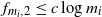 $f_{m_i,2}\le c\log m_i$
and then after
$f_{m_i,2}\le c\log m_i$
and then after
 $j-1$
jumps the time is at most
$j-1$
jumps the time is at most
 $\Delta\,:\!=\,f_{m_i,2}+\theta(\,j-1) \le c$
 $\log m_i+\theta(\,j-1)$
, and the probability of not having a single tree by this time is
$\log m_i+\theta(\,j-1)$
, and the probability of not having a single tree by this time is
 $\mathrm{e}^{-\Delta}$
.
$\mathrm{e}^{-\Delta}$
.
Together with (12) this yields
 \begin{align}\left(m_{i+1}- m_i\right) 1_{i\ge\kappa} \preccurlyeq \sum_{j=1}^{N_i} \xi_{i,j},\end{align}
where
 $X \preccurlyeq Y$
means that Y stochastically dominates X. Let
$X \preccurlyeq Y$
means that Y stochastically dominates X. Let
 \begin{align*}\mathcal{B}_i\,:\!=\,\Bigg\{\sum_{j=1}^{N_i}\xi_{i,j}\ge m_i^{c+\epsilon/2}\times c_1\log i\Bigg\}\supseteq\Bigg\{\sum_{j=1}^{N_i}\xi_{i,j}\ge m_i^{c+\epsilon}-m_i\Bigg\}\end{align*}
for large i (the inclusion follows from part (a)). Then, using (13), for
 $i\ge \kappa$
,
$i\ge \kappa$
,
 \begin{align}\begin{split}\mathrm{P}\big(\mathcal{B}_i\mid \mathcal{F}_{f_{m_i+1,1}}\big)&\le\mathrm{P}\big(\mathcal{B}_i\mid N_i\le c_1 \log i\mid \mathcal{F}_{f_{m_i+1,1}}\big)+\mathrm{P}\big(N_i>c_1 \log i\mid \mathcal{F}_{f_{m_i+1,1}}\big)\\[4pt] & \le\mathrm{P}\big( \xi_{i,j}\ge m_i^{c+\epsilon/2} \text{ for some }j=1,2,\ldots,\lfloor c_1\log i\rfloor\big)+\frac1{i^2}\\[4pt] & \le c_1\log i \times \max_{j\le c_1\log i}\mathrm{P}\big( \xi_{i,j}\ge m_i^{c+\epsilon/2} \big)+\frac1{i^2}.\end{split}\end{align}
Since
 \begin{align*}\mathrm{P}\big(\xi_{i,j}> m_i^{c+\epsilon/2}\big)\le \bigg(1-\frac1{m_i^c \mathrm{e}^{\theta (\,j-1)}}\bigg)^{m_i^{c+\epsilon/2}}\le \exp\big(-\mathrm{e}^{-\theta(\,j-1)}\, m_i^{\epsilon/2}\big)\le \exp\bigg(-\frac{m_i^{\epsilon/2}}{i^{c_1\theta}}\bigg)\end{align*}
as
 $j\le c_1\log i$
, and by part (a) of the lemma
$j\le c_1\log i$
, and by part (a) of the lemma
 $m_i$
grows faster than
$m_i$
grows faster than
 $i^r$
for any
$i^r$
for any
 $r>0$
, the right-hand side of (15) is summable over i, and thus the events
$r>0$
, the right-hand side of (15) is summable over i, and thus the events
 $\left\{\sum_{j=1}^{N_i}\xi_{i,j}\ge m_i^{c+\epsilon}-m_i\right\}$
happen finitely often by the Borel–Cantelli lemma. As a result, from (14),
$\left\{\sum_{j=1}^{N_i}\xi_{i,j}\ge m_i^{c+\epsilon}-m_i\right\}$
happen finitely often by the Borel–Cantelli lemma. As a result, from (14),
 \begin{align*}m_{i+1}\le m_i^{c+\epsilon}\end{align*}
for all large i a.s.
Proof of Theorem
4.2. Fix some
 $\epsilon>0$
. Lemma 4.3 implies that
$\epsilon>0$
. Lemma 4.3 implies that
 $\log m_{i+1}\le (1+\epsilon) \log m_i$
for all large i, a.s. On the other hand, by Lemma 4.1,
$\log m_{i+1}\le (1+\epsilon) \log m_i$
for all large i, a.s. On the other hand, by Lemma 4.1,
 $f_{m_{i+1},1}\le (1+\epsilon) \log m_{i+1}$
. Hence, for all
$f_{m_{i+1},1}\le (1+\epsilon) \log m_{i+1}$
. Hence, for all
 $n \in \{m_i,\ldots,m_{i+1}\}$
we have
$n \in \{m_i,\ldots,m_{i+1}\}$
we have
 \begin{align*}f_{n,1}\leq f_{m_{i+1},1}\le (1+\epsilon)^2\log{m_i}\le (1+\epsilon)^2 \log{n}.\end{align*}
Together with Lemma 4.2, this implies
 $f_{n,1} =\mathcal{O}(\log n)$
.
$f_{n,1} =\mathcal{O}(\log n)$
.
The next statement strengthens part (a) of Lemma 4.3 (without using Conjecture 4.1).
Theorem 4.3. There exists an
 $\alpha>0$
such that
$\alpha>0$
such that
 $m_i\ge \exp(\!\exp(\alpha i))$
for all large i a.s.
$m_i\ge \exp(\!\exp(\alpha i))$
for all large i a.s.
Proof. Fix some
 $\epsilon>0$
, and denote
$\epsilon>0$
, and denote
 $\mathrm{P}_*(\cdot)=\mathrm{P}(\cdot\mid \mathcal{F}_{f_{m_{i},1}})$
, the conditional probability measure based on the information available until the first time
$\mathrm{P}_*(\cdot)=\mathrm{P}(\cdot\mid \mathcal{F}_{f_{m_{i},1}})$
, the conditional probability measure based on the information available until the first time
 $m_i$
was burnt; thus
$m_i$
was burnt; thus
 $\mathcal{F}_{f_{m_{i},1}}$
is a stopped sigma-algebra.
$\mathcal{F}_{f_{m_{i},1}}$
is a stopped sigma-algebra.
First, we want to estimate the time difference between the second and the first fires which burnt the next maximum site
 $m_{i+1}$
. Define
$m_{i+1}$
. Define
 \begin{align*}A_i=\{\,f_{m_{i+1},2}-f_{m_{i+1},1}\ge 2\epsilon\log m_i\}\end{align*}
and recall the definitions of
 $F_n$
from Lemma 4.2,
$F_n$
from Lemma 4.2,
 $B_i$
from (10) and
$B_i$
from (10) and
 $C_i$
from (13); the event
$C_i$
from (13); the event
 $C_i$
is independent of
$C_i$
is independent of
 $\mathcal{F}_t$
, while the event
$\mathcal{F}_t$
, while the event
 $F_{m_i}$
is
$F_{m_i}$
is
 $\mathcal{F}_t$
-measurable.
$\mathcal{F}_t$
-measurable.
On
 $F_{m_i}$
, we have
$F_{m_i}$
, we have
 $f_{m_{i+1},1}>f_{m_i,1}\ge(1-\epsilon)\log m_i$
. Let us now estimate
$f_{m_{i+1},1}>f_{m_i,1}\ge(1-\epsilon)\log m_i$
. Let us now estimate
 $\mathrm{P}_*\left(A_i^c\mid F_{m_i}\right)$
. The fire which reached
$\mathrm{P}_*\left(A_i^c\mid F_{m_i}\right)$
. The fire which reached
 $m_{i+1}$
for the first time is also the one which reached sites
$m_{i+1}$
for the first time is also the one which reached sites
 $x\in (m_{i},m_{i+1}]$
for the first time. Recall that
$x\in (m_{i},m_{i+1}]$
for the first time. Recall that
 $N_i$
denotes the number of jumps of this fire on these positions; from the proof of part (b) of Lemma 4.3 it follows that with probability
$N_i$
denotes the number of jumps of this fire on these positions; from the proof of part (b) of Lemma 4.3 it follows that with probability
 $\ge 1-1/i^2$
the event
$\ge 1-1/i^2$
the event
 $C_i=\{N_{i}\le \lfloor c\log i\rfloor\}\subseteq \{\mathrm{e}^{\theta N_{i}}\le i^{c\theta}\}$
occurs (we are putting an upper bound on the number of jumps in a fire and this fact did not require Conjecture 4.1).
$C_i=\{N_{i}\le \lfloor c\log i\rfloor\}\subseteq \{\mathrm{e}^{\theta N_{i}}\le i^{c\theta}\}$
occurs (we are putting an upper bound on the number of jumps in a fire and this fact did not require Conjecture 4.1).
For
 $f_{m_{i+1},2}-f_{m_{i+1},1}$
to be smaller than
$f_{m_{i+1},2}-f_{m_{i+1},1}$
to be smaller than
 $2\epsilon \log m_i$
, at least one tree must appear during the time interval
$2\epsilon \log m_i$
, at least one tree must appear during the time interval
 $[\,f_{m_{i+1},1}-\theta N_i,f_{m_{i+1},1}+2\epsilon \log m_i]$
at each location
$[\,f_{m_{i+1},1}-\theta N_i,f_{m_{i+1},1}+2\epsilon \log m_i]$
at each location
 $x\in [m_i,m_{i+1})$
(the term
$x\in [m_i,m_{i+1})$
(the term
 $(-\theta N_i)$
corresponds to the fact that there are up to
$(-\theta N_i)$
corresponds to the fact that there are up to
 $N_i$
jumps among these positions), and the probability of this event is at most
$N_i$
jumps among these positions), and the probability of this event is at most
 $\left(1-{1}/{m_i^{2\epsilon}\, \mathrm{e}^{N_i\theta}}\right)$
for each of these sites, independently of the others. Hence,
$\left(1-{1}/{m_i^{2\epsilon}\, \mathrm{e}^{N_i\theta}}\right)$
for each of these sites, independently of the others. Hence,
 \begin{align*}\mathrm{P}_*(A_i^c\mid F_{m_i})&\le \mathrm{P}_*(\text{tree appears at all} \,x\, \text{for } m_i \lt x\le m_{i+1}\mid F_{m_i})\\[4pt]&\le \mathrm{P}_*(\text{tree appears at all}\, x \,\text{for} m_i \lt x\le m_{i+1}\mid B_i,F_{m_i})+\mathrm{P}_*(B_i^c\mid F_{m_i})\\[4pt]&\le \mathrm{P}_*(\text{tree appears at all} \,x\, \text{for} m_i \lt x\le m_{i+1}\mid B_i,C_i,F_{m_i}) \\[4pt]& +\mathrm{P}(C_i^c\mid F_{m_i})+\mathrm{P}_*(B_i^c\mid F_{m_i})\\[4pt]& \le\left(1-\frac{1}{m_i^{2\epsilon}\, \mathrm{e}^{\theta c\log i}}\right)^{m_i^{1-\epsilon}}+\frac1{i^2}+(1-c')= \left(1-\frac{1}{m_i^{2\epsilon}\, i^{c\theta}}\right)^{m_i^{1-\epsilon}}+\frac1{i^2}+1-c'\\[4pt] &\le \exp\left\{-\frac{m_i^{1-3\epsilon}}{ i^{c\theta}}\right\} +1-2 c'' \quad\text{for large }i.\end{align*}
for some
 $c''>0$
, since on
$c''>0$
, since on
 $B_i$
we have
$B_i$
we have
 $m_{i+1}-m_i\ge m_i^{1-\epsilon}$
, and using (11).
$m_{i+1}-m_i\ge m_i^{1-\epsilon}$
, and using (11).
The longer the time interval between the first and second fire at
 $m_{i+1}$
(as implied by the event
$m_{i+1}$
(as implied by the event
 $A_i$
), the greater the probability that it will burn at least
$A_i$
), the greater the probability that it will burn at least
 $m_i^{1+\epsilon/2}$
additional sites. Hence, if both
$m_i^{1+\epsilon/2}$
additional sites. Hence, if both
 $F_{m_i}$
and
$F_{m_i}$
and
 $A_i$
occur, the probability that the second fire to arrive at
$A_i$
occur, the probability that the second fire to arrive at
 $m_{i+1}$
will also stop before immediately burning additional
$m_{i+1}$
will also stop before immediately burning additional
 $m_i^{1+\epsilon/2}$
sites equals
$m_i^{1+\epsilon/2}$
sites equals
 \begin{align}&\mathrm{P}_*(\,f_{m_{i+1}+k,1}> f_{m_{i+1},2}\text{ for some }k\in [1,m_i^{1+\epsilon/2}]\mid F_{m_i},A_i)\nonumber\\&\le\mathrm{P}_*(\,f_{m_{i+1}+1,1}> f_{m_{i+1},2}\mid F_{m_i},A_i)+\sum_{k=2}^{m_i^{1+\epsilon/2}}\mathrm{P}_*(\,f_{m_{i+1}+k,1}> f_{m_{i+1},2}\mid F_{m_i},A_i)\nonumber\\&\qquad \le\frac{\mathrm{e}^{-\theta}}{m_i^{2\epsilon}}+\frac{m_i^{1+\epsilon/2}}{m_i^{1+\epsilon}}\le \frac{2}{m_i^{\epsilon/2}}\end{align}
(when
 $m_i$
is large). The first term in the above inequality corresponds to the probability that a tree appeared at position
$m_i$
is large). The first term in the above inequality corresponds to the probability that a tree appeared at position
 $m_{i+1}+1$
during the time interval
$m_{i+1}+1$
during the time interval
 \begin{align*}[\,f_{m_{i+1},1}+\theta, f_{m_{i+1},2}]\supseteq [\,f_{m_{i+1},1}+\theta, f_{m_{i+1},1}+2\epsilon \log m_i],\end{align*}
while the second term corresponds to the event that at least one of the locations
 $m_{i+1}+2,$
 $m_{i+1}+3,\ldots,m_{i+1}+m_i^{1+\epsilon/2}$
remains vacant, and we know that the probability of such a site to remain vacant is
$m_{i+1}+3,\ldots,m_{i+1}+m_i^{1+\epsilon/2}$
remains vacant, and we know that the probability of such a site to remain vacant is
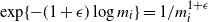 $\exp\{-(1+\epsilon)\log m_i\}=1/m_i^{1+\epsilon}$
. Since
$\exp\{-(1+\epsilon)\log m_i\}=1/m_i^{1+\epsilon}$
. Since
 $F_{m_i}$
is
$F_{m_i}$
is
 $\mathrm{P}_*$
-measurable, using (16) we have
$\mathrm{P}_*$
-measurable, using (16) we have
 \begin{align*}\mathrm{P}_*(m_{i+2}- m_i\ge m_i^{1+\epsilon/2})&\ge\mathrm{P}_*(m_{i+2}- m_i\ge m_i^{1+\epsilon/2}, A_i, F_{m_i})\\[3pt] &=\mathrm{P}_*(m_{i+2}- m_i\ge m_i^{1+\epsilon/2}\mid A_i, F_{m_i})\, \mathrm{P}_*( A_i\mid F_{m_i}) \, \mathrm{P}_*( F_{m_i})\\[3pt] &\ge \bigg(1-\frac2{m_i^{\epsilon/2}}\bigg)\cdot\left(2c''-\exp\left\{-\frac{m_i^{1-3\epsilon}}{2\, i^{c\theta}}\right\} \right)1_{F_{m_i}}\\[3pt] & \ge c''\cdot 1_{F_{m_i}} \cdot 1_{m_i>i^r}\end{align*}
for some fixed non-random
 $r>1$
and all large i. Now the inequality
$r>1$
and all large i. Now the inequality
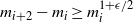 $m_{i+2}- m_i\ge m_i^{1+\epsilon/2}$
implies
$m_{i+2}- m_i\ge m_i^{1+\epsilon/2}$
implies
 \begin{align}\log m_{i+2}\ge \left(1+\frac{\epsilon}2\right)\log m_i\quad\Longrightarrow\quad\log\log m_{i+2}-\log\log m_i\ge \log \left(1+\frac{\epsilon}2\right)=:\epsilon'>0.\end{align}
Setting
 $i=2j$
,
$i=2j$
,
 $j=1,2,\ldots$
, we conclude that we can construct an i.i.d. sequence of Bernoulli(c”) random variables
$j=1,2,\ldots$
, we conclude that we can construct an i.i.d. sequence of Bernoulli(c”) random variables
 $\xi_j$
such that
$\xi_j$
such that
 \begin{align*}\log\log m_{2(\,j+1)}-\log\log {m_{2j}}\ge \epsilon' \xi_j\cdot 1_{F_{m_{2j}}} \cdot 1_{m_{2j}>(2j)^r}.\end{align*}
By Lemma 4.3
 $m_i>i^r$
for any fixed r and all sufficiently large i; we also know that the events
$m_i>i^r$
for any fixed r and all sufficiently large i; we also know that the events
 $F_{m_i}^c$
occur only finitely often a.s. yielding
$F_{m_i}^c$
occur only finitely often a.s. yielding
 \begin{align*} \liminf_{k\to\infty} \frac{\log\log m_{2k}}k &=\liminf_{k\to\infty} \frac{\sum_{j=1}^{k-1}\left(\log\log m_{2j+2}-\log\log m_{2j}\right)}k \\ & \ge \liminf_{k\to\infty} \frac{\displaystyle\sum_{j=1}^{k-1}\epsilon'\xi_j 1_{F_{m_{2j}}} 1_{m_{2j}>(2j)^r}}k =\epsilon'\lim_{k\to\infty} \frac{\displaystyle\sum_{j=1}^{k-1}\xi_j}k=\epsilon'c''>0\qquad \text{a.s.} \end{align*}
(please compare this with the proof of part (a) of Lemma 4.3) from which it follows that for some
 $\alpha>0$
we have
$\alpha>0$
we have
 $m_i\ge \exp\left\{\mathrm{e}^{\alpha i}\right\}$
for all sufficiently large i a.s.
$m_i\ge \exp\left\{\mathrm{e}^{\alpha i}\right\}$
for all sufficiently large i a.s.


Acknowledgements
We would like to thank the anonymous referees for their comments, and especially for providing us with relevant references.
Funding information
The research is supported by Swedish Research Council grant VR 2019-04173 and Crafoord Foundation grant 20190667.
Competing interests
There were no competing interests to declare which arose during the preparation or publication process of this article.


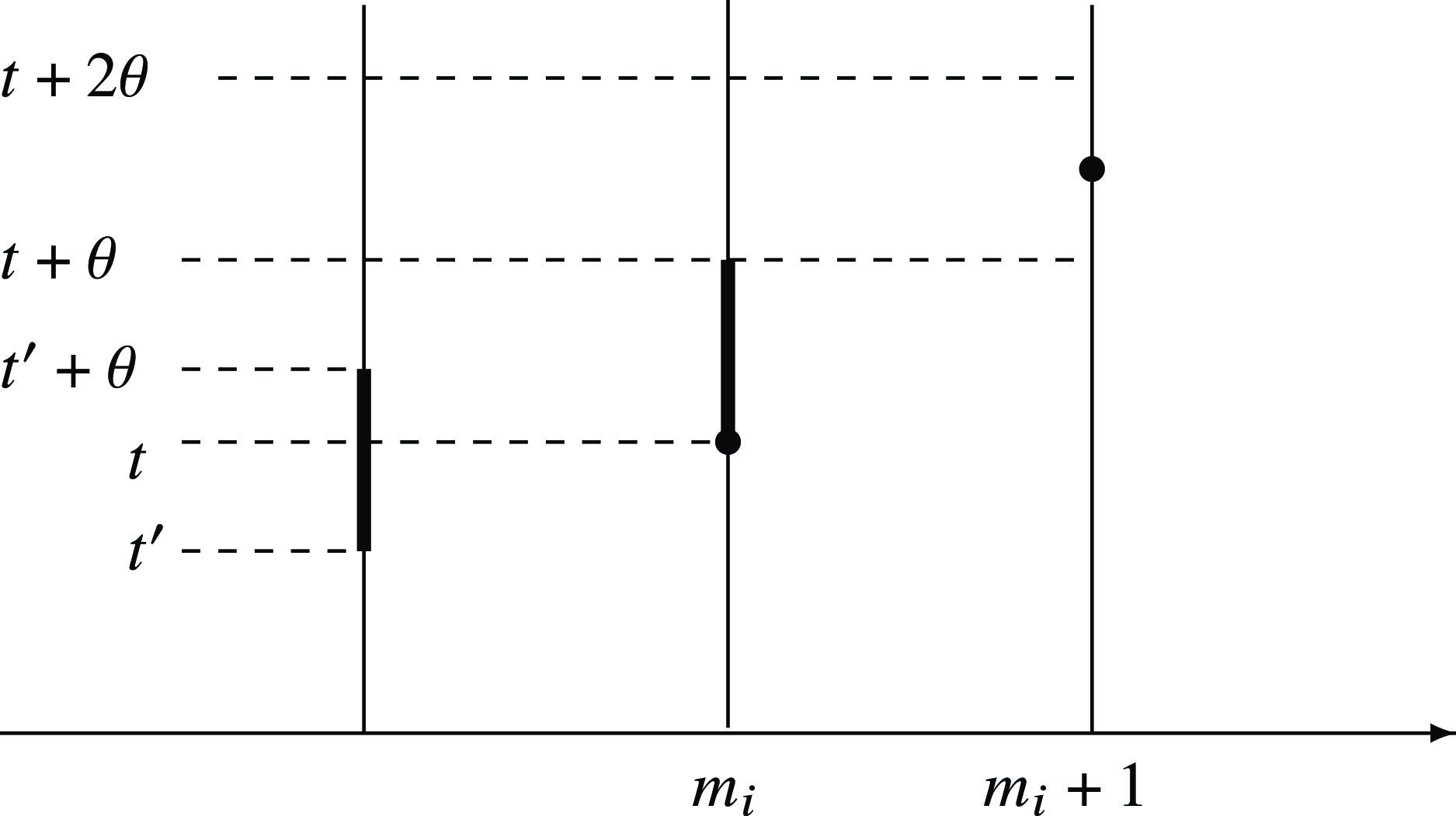


 Open access