


1. Introduction
Climate change, partly driven by rising emissions, has damaging and often irreversible impacts on entire economies. Investigating the influence of economic decisions on the evolution of environmental quality becomes crucial. This question must be addressed by considering how environmental variables evolve over time and how economic activities, natural processes, and policy interventions influence them. This approach captures the complex and interrelated nature of environmental systems and it allows researchers and policymakers to forecast changes, evaluate the effectiveness of interventions, and design sustainable management strategies. In particular, production and the environment are intricately linked, with constant feedback shaping how firms operate and how ecosystems respond: in fact, pollution is very often a by-product of the economic process, with significant negative effects on environmental quality. Reducing pollution from production is a key global and European Union (EU) environmental goal. The European Green Deal aims to make Europe climate neutral by 2050, boost the economy through green technology, create sustainable industry and transport, and cut pollution. Turning climate and environmental challenges into opportunities will make the transition just and inclusive for all. The European Commission helps EU Member States design and implement reforms that support the green transition and that contribute to achieving the goals of the European Green Deal.Footnote 1 At both a global level and within the EU, a variety of policies, initiatives, and frameworks have been implemented to address the environmental impacts of industrial and agricultural production, with a particular focus on reducing greenhouse gas emissions, waste, water, and air pollution, and transitioning towards a more sustainable and circular economy. Globally, various international agreements and initiatives have been established to guide nations and industries toward reducing pollution from production: the Paris Agreement (2015) aims to limit global warming and to reduce carbon emissions; the United Nations Sustainable Development Goals (The 2030 Agenda for Sustainable Development - SDGs) aims to ensure sustainable production patterns and significantly reduce waste and pollution and to encourage firms to adopt cleaner, more efficient technologies to reduce pollution and mitigate climate change; the EU has set ambitious goals to reduce pollution from production, primarily through the European Green Deal and supporting regulatory frameworks. Key objectives include reducing emissions, promoting circular economy principles, and green transition. Regarding the reduction of the production’s emissions, the Zero Pollution Action Plan (2021) aims for “zero pollution” of air, water and soil by 2050. It includes measures to reduce pollution from industrial emissions, hazardous chemicals, and waste management. As mentioned previously, one of the main drivers for pollution is the production process: in fact, production processes, when inefficient or unregulated, lead to significant pollution across air, water, and soil, causing environmental degradation and impacting human health. Hence, sustainable production methods, energy efficiency, waste reduction, and stricter environmental regulations can help mitigate these effects. The green transition toward a cleaner economy requires significant investments from businesses in green technologies, a shift that may lead to higher costs and reduced profitability for the companies themselves (see, e.g., Morgenstern et al. (Reference Morgenstern, Pizer and Shih2001), Rodrik (Reference Rodrik2014), and Radi and Westerhoff (Reference Radi and Westerhoff2024)).
These government regulations and policies are key to mitigating pollution, promoting sustainable practices, and improving environmental quality worldwide. By enforcing these rules, governments push industries and individuals to adopt greener technologies, reduce waste, and curb emissions. For example, the EU Emissions Trading System (ETS) aims to reduce the greenhouse gas emissions of industrial sectors through a cap-and-trade system, by allocating emission allowances to companies: if companies emit less than allowed, they can sell the excess, but if they exceed it, they have to buy additional permits. In this context, a gradually decreasing cap on emissions forces industries to adopt cleaner technologies over time.
In the present work, we consider a setup in which firms can choose to use green technology, following government regulations, thus implying no pollution, or to behave dishonestly, that is, to be a polluting firm. Then economic decisions of firms influence environmental quality through the non-compliant behavior of the firms themselves.
To take into account non-compliant behavior, we consider a production process involving a level of emissions that depends on the type of technology used by the firm. If the firm makes products using cleaner technology (e.g., purification systems etc.) it will incur higher production costs than if it uses less emission-conscious technology. Environmental legislation requires firms to use the least polluting technology, but the firm may behave dishonestly by contravening legal requirements and using the most polluting technology in order to incur lower production costs.
In this context, the choice is made based on rational behavior: the firm decides whether to be environmentally compliant by comparing the expected benefits of being dishonest (lower production costs) with the expected costs if the non-compliant behavior is discovered and therefore punished (enforcement channel). In fact, the drive towards more sustainable growth, in particular through the achievement of higher environmental quality, has led to the setting of stricter production standards, especially with regard to the levels of pollution allowed in companies. This change has strengthened environmental governance by introducing environmental regulations, emission taxes, inspections, and penalties, which have proven effective in improving policymakers’ ability to control pollution (e.g., Neves et al. (Reference Neves, Marques and Patrício2020)).
The model is formalized through a word-of-mouth mechanism (see, e.g., Dawid (Reference Dawid1999) and Lamantia and Pezzino (Reference Lamantia and Pezzino2021)) according to which firms interact and change their type (from polluting to nonpolluting or vice versa) depending on the behavior of the other firms and on the sensibility toward the environmental quality.Footnote 2 In line with the standard approach of evolutionary dynamics, each period firms are matched in pairs, and through this matching they learn about pay-off of other firms. This type of interaction can play a significant role in shaping public perception and behavior regarding environmental issues. In fact, environmental quality depends greatly on the behavior of the majority agents: the individual is aware of the limited environmental impact of his choices. So, if most firms pollute, the fact that a given firm decides not to pollute will have a small impact on environmental quality. This social “conditioning” mechanism represents the environmental context well: if everyone pollutes, I will too. Vice versa, positive discussions about environmental quality can raise awareness about sustainability practices, encouraging individuals and communities to adopt greener habits.Footnote 3
In this context, the attitude toward greenery plays a crucial role, as it affects the measure in which a firm changes type from nonpolluting to polluting. To take into account such an attitude, we consider an asymmetric scheme as firstly proposed by Bose et al. (Reference Bose, Capasso and Murshid2008) and introduce the propensity for greenery: greater inherent propensity for greenery stems from the higher value attached to the environmental quality. From the propensity for greenery assumption, all polluting firms interacting with nonpolluting ones choose to change behavior only if the expected profit from honesty exceeds that of dishonesty. Conversely, not all nonpolluting firms interacting with polluting ones opt to change behavior, even if the higher expected profit is attainable, thus it depends on the inherent attitude to environmental quality preservation. This attitude is a factor that a government can influence, but only over the medium to long term.
The State entrusts environmental inspectors to ensure that firms comply with the law. The monitoring effort, that is, the probability a firm incurs in control by the State, is updated at any time by considering the expected variation in the environmental quality level. More precisely, the level of monitoring put in place by the State depends on both the variation in the environmental quality level in the economy and on the previous level of monitoring. This consideration stems from the realization that there is an “inertia” in the expenditure items of the public budget, since some of them refer to multiyear expenditure commitments that cannot be completely changed from one year to the next (as in Coppier et al. (Reference Coppier, Michetti and Panchuk2024)).
Regarding the evolution of environmental quality, we consider an index that depends on the environmental quality of the previous period, on the presence of firms that pollute by breaking environmental rules, and, following Caravaggio and Sodini (Reference Caravaggio and Sodini2023), on a natural level of environmental quality (no polluting case) that can be reached without human activity.
The main scope of the present work is to describe the evolution of polluting behavior and of environmental quality and to explain if and to what extent they are influenced by external and internal channels, that is, the enforcement channel and the propensity for greenery channel. The former accounts for the effort made by the State to control the firm’s behavior and apply a fine if a dishonest polluting firm is discovered. The latter considers the likelihood with which a green firm decides to become nongreen depending on the propensity for greenery representing the different attitudes of firms towards environmental quality.
Putting together such ingredients we obtain a 3D piecewise-smooth dynamical system in discrete time, describing the evolution of the fraction of polluting firms, the monitoring level by the State, and the environmental quality over time. We describe the long-run evolution of such a model both from the qualitative and quantitative points of view, depending on the enforcement under different inner propensities for greenery.
Our main results identify three distinct scenarios based on the level of firms’ propensity for greenery. These scenarios can be summarized as follows.
-
• High propensity for greenery: if firms have a strong inclination toward green practices, and the system does not start from a state where all firms are non-compliant, then there exist internal mechanisms that naturally drive the system toward an equilibrium where all firms comply, resulting in the highest possible environmental quality. The State can promote this desirable outcome through policies that enhance firms’ environmental awareness, potentially using economic incentives, and investing in technologies that reduce the production costs of green alternatives.
-
• Intermediate propensity for greenery: if firms show a moderate inclination toward environmentally friendly practices—sufficient to allow for positive outcomes but not strong enough to guarantee them. Under these conditions, the system may either reach a good equilibrium with high environmental quality or fall into a “dishonesty trap”, that is, an equilibrium where all firms are non-compliant and environmental quality is at its lowest.
-
• Low propensity for greenery: if firms have a low inclination toward green practices, additional internal equilibria can arise where compliant and non-compliant firms coexist. The range of these mixed equilibria grows as the concern for environmental practices rises. Here, adjustments in regulatory factors, such as the fine attached to non-compliant behavior and the responsiveness of monitoring environmental quality changes, affect equilibrium outcomes.
Each scenario highlights different paths through which regulatory and economic interventions can help foster an environment of greater compliance and improved environmental quality.
The paper is organized as follows. In Section 2 we describe the model setup. In Section 3 we perform the qualitative and quantitative dynamic study. Section 4 concludes the paper.
2. Model setup
2.1 Firms
The production process involves a level of emissions that depends on the technology used by the firms. If the firm makes products using clean technology (e.g., purification systems etc.) it will incur higher production costs than if it uses less emission-conscious technology. The two different technologies entail different costs: the high-emission technology entails a production cost $c^l$
, while the legally prescribed low-emission technology entails a higher production cost
$c^l$
, while the legally prescribed low-emission technology entails a higher production cost $c^h$
, being
$c^h$
, being $c^h\gt c^l\gt 0$
.
$c^h\gt c^l\gt 0$
.
The firm may decide to behave dishonestly by contravening legal requirements and using the most polluting technology (prohibited by law) to incur lower production costs. The State entrusts environmental inspectors with the task of checking that firms comply with the environmental regulation.
Following previous works such as Coppier et al. (Reference Coppier, Grassetti and Michetti2021) and Panchuk et al. (Reference Panchuk, Sushko, Michetti and Coppier2022), we consider a discrete-time setup, that is, $t=0,1,2,\ldots$
, and define
$t=0,1,2,\ldots$
, and define $x_t\in [0,1]$
as the fraction of firms making products using high-emission technology (dishonest firms) at time
$x_t\in [0,1]$
as the fraction of firms making products using high-emission technology (dishonest firms) at time $t$
.
$t$
.
The State monitors companies to verify that they use low-emission clean technology. Let $q_t$
be the monitoring level put in place by the State at time
$q_t$
be the monitoring level put in place by the State at time $t$
to detect the presence of polluting firms, while
$t$
to detect the presence of polluting firms, while $q^e_t\in [0,1]$
represents the expected probability by the firm, at any time
$q^e_t\in [0,1]$
represents the expected probability by the firm, at any time $t$
, of being monitored, according to the expected control level fixed by the State and, then, of being reported. If a dishonest firm is monitored and detected, it is punished with a fine being a fraction
$t$
, of being monitored, according to the expected control level fixed by the State and, then, of being reported. If a dishonest firm is monitored and detected, it is punished with a fine being a fraction $f\gt 0$
of the capital level, thus linked to the production level.
$f\gt 0$
of the capital level, thus linked to the production level.
We assume for simplicity a linear technology of the kind $y_t=A k_t$
, and, without loss of generality, a unitary price of produced good. Then, by taking into account the previous considerations, we derive the expected profit at time
$y_t=A k_t$
, and, without loss of generality, a unitary price of produced good. Then, by taking into account the previous considerations, we derive the expected profit at time $t$
of an honest firm (using low-emission technology) as
$t$
of an honest firm (using low-emission technology) as
 \begin{equation} E[\pi _{h,t}] = \pi _{h,t} = Ak_t - c^hk_t, \quad A \gt c^h \gt 0. \end{equation}
On the other hand, the expected profit at time $t$
of a dishonest firm (using a high-emission technology) depends also on the event of being discovered fraudulent, that is,
$t$
of a dishonest firm (using a high-emission technology) depends also on the event of being discovered fraudulent, that is,
 \begin{equation} \pi _{d,t} = \left \{ \begin{array}{l@{\quad}l} \pi _{d,NM,t}=Ak_t-c^lk_t, & \hbox{if not monitored,} \\ \pi _{d, M,t}= Ak_t-c^hk_t-fk_t, & \hbox{if monitored}, \end{array}\right . \end{equation}
being $A \gt c^l+f$
the total productivity factor. Since the monitoring level may change at any time
$A \gt c^l+f$
the total productivity factor. Since the monitoring level may change at any time $t$
, the expected profit at time
$t$
, the expected profit at time $t$
for a dishonest firm is given by
$t$
for a dishonest firm is given by
 \begin{equation} E[\pi _{d,t}] = q^e_t\pi _{d, M,t}+(1-q^e_t)\pi _{d,NM,t}= Ak_t-q^e_tc^hk_t-fq^e_tk_t- (1-q^e_t)c^lk_t. \end{equation}
Therefore, the firm will find it worthwhile to pollute, that is, use high-emission technology, if
 \begin{equation} q^e_t\lt \frac {\Delta _c}{\Delta _c+ f}, \end{equation}
where $\Delta _c=c^h-c^l\gt 0$
.
$\Delta _c=c^h-c^l\gt 0$
.
The difference in expected profits between polluting and nonpolluting firms is then given by
 \begin{equation} \gamma (q^e_t) = E[\pi _{d,t}] - \pi _{h,t} = (1 - q^e_t) \Delta _c k_t - fq^e_tk_t \end{equation}
and can be rewritten in terms of a unit of capital $k_t$
, thus implying the following expression
$k_t$
, thus implying the following expression
 \begin{equation} \delta (q^e_t) = \frac {E[\pi _{d,t}] - \pi _{h,t}}{k_t} = (1 - q^e_t) \Delta _c - f q^e_t, \end{equation}
being a linear strictly decreasing function of the expected monitoring level. In such a way, the difference between expected profits decreases as the expected monitoring level increases, while the fine level affects the intensity of change.
2.2 Environment
We now specify the environmental quality evolution through an environmental quality index often used as a measure of the overall quality of the environment at a given time $t$
(see, e.g., John and Pecchenino (Reference John and Pecchenino1994) and Zhang (Reference Zhang1999)). This index can encompass various indicators such as air and water quality, greenhouse gas emissions, biodiversity, and ecosystem health, among others, and provides a single value that reflects the current state of environmental quality. By taking into account Grassetti et al. (Reference Grassetti, Mammana and Michetti2024), natural resources and ecosystems at time
$t$
(see, e.g., John and Pecchenino (Reference John and Pecchenino1994) and Zhang (Reference Zhang1999)). This index can encompass various indicators such as air and water quality, greenhouse gas emissions, biodiversity, and ecosystem health, among others, and provides a single value that reflects the current state of environmental quality. By taking into account Grassetti et al. (Reference Grassetti, Mammana and Michetti2024), natural resources and ecosystems at time $t$
are described by the index of the environmental quality denoted by
$t$
are described by the index of the environmental quality denoted by $E_t \geq 0$
.
$E_t \geq 0$
.
As in Caravaggio and Sodini (Reference Caravaggio and Sodini2023), there exists a given natural level of environmental quality related to the nonpolluting case that can be asymptotically reached without human activity. Without loss of generality, we set such a level to $1$
, representing the maximum level of environmental quality that could be reached. Obviously, in the presence of polluting firms, the environmental quality will be reduced.
$1$
, representing the maximum level of environmental quality that could be reached. Obviously, in the presence of polluting firms, the environmental quality will be reduced.
Similarly to what has been proposed in Caravaggio and Sodini (Reference Caravaggio and Sodini2023), by taking into account these factors, we assume that the environmental quality index evolves according to
 \begin{equation} E_{t+1} = E_t + b(1 - E_t) - ax_t \stackrel {df}{=} S_3(x_t, E_t), \end{equation}
where the environmental level $1$
represents the value toward that the index tends when the fraction of polluting firms is zero for all
$1$
represents the value toward that the index tends when the fraction of polluting firms is zero for all $t$
, the parameter
$t$
, the parameter $b \in (0, 1)$
measures the speed of reversion of the environmental quality to
$b \in (0, 1)$
measures the speed of reversion of the environmental quality to $1$
, and the parameter
$1$
, and the parameter $a\in (0,b)$
measures the strength of environmental degradation due to the presence of polluting firms. Notice that condition
$a\in (0,b)$
measures the strength of environmental degradation due to the presence of polluting firms. Notice that condition $b \in (0, 1)$
guarantees the existence of an endogenous mechanism that leads the environment to the equilibrium level in the absence of polluting firms. In contrast, condition
$b \in (0, 1)$
guarantees the existence of an endogenous mechanism that leads the environment to the equilibrium level in the absence of polluting firms. In contrast, condition $a\in (0,b)$
is necessary to ensure that the environmental level cannot become negative, even in the presence of polluting firms.
$a\in (0,b)$
is necessary to ensure that the environmental level cannot become negative, even in the presence of polluting firms.
2.3 State
The State monitors firms in order to detect and punish polluting behavior. Note that in previous works such as Bose et al. (Reference Bose, Capasso and Murshid2008) and Coppier et al. (Reference Coppier, Grassetti and Michetti2021) it has been assumed that the State fixes the monitoring level to be set at time $t+1$
by observing the fraction of dishonest firms at time
$t+1$
by observing the fraction of dishonest firms at time $t$
. In a similar way, the updating control level put in place by the State is assumed to be modified (decreased or increased) starting from the existing level of audit and considering the environmental quality level in the economy to put in place an effective strategy for combating pollution.
$t$
. In a similar way, the updating control level put in place by the State is assumed to be modified (decreased or increased) starting from the existing level of audit and considering the environmental quality level in the economy to put in place an effective strategy for combating pollution.
In fact, monitoring activities require human and monetary resources that cannot be completely renewed from one period to another, there exists an “inertia” in the expenditure items of the public budget. Hence, as in Coppier et al. (Reference Coppier, Michetti and Panchuk2024), the level of control put in place is updated starting from the existing level of audit. In addition, the future level of monitoring depends on the environmental quality in the economy or the fraction of polluting firms. Since a higher fraction of polluting firms implies a lower environmental level, then we consider that the monitoring level increases as long as the environmental quality is decreased, and vice versa. As in Coppier et al. (Reference Coppier, Michetti and Panchuk2024), we assume rational expectations, that is, the State knows the future fraction of polluting firms, and hence the environmental quality level variation $E_{t+1}-E_{t}$
depending on the fraction of dishonest firms in the economy at time
$E_{t+1}-E_{t}$
depending on the fraction of dishonest firms in the economy at time $t$
.
$t$
.
To reflect the previous arguments, a simple rule of thumb to describe the updating control strategy can be that the monitoring level is modified so that the growth rate is proportional to the change in environmental quality. To the scope we suggest the following rule
 \begin{equation} q_{t+1} = G(q_t, \Delta E_t) = q_t\left (1 - d\Delta E_t \right ), \end{equation}
where $\Delta E_t=E_{t+1}-E_t$
, that is,
$\Delta E_t=E_{t+1}-E_t$
, that is, $\Delta E_t \gt 0$
if from the time
$\Delta E_t \gt 0$
if from the time $t$
to
$t$
to $t+1$
the environmental quality is increased, and vice versa. Parameter
$t+1$
the environmental quality is increased, and vice versa. Parameter $d\in (0,1)$
has been introduced to capture the intensity with which
$d\in (0,1)$
has been introduced to capture the intensity with which $q_t$
can grow/decline from time
$q_t$
can grow/decline from time $t$
to time
$t$
to time $t+1$
in response to higher/lower observed environmental quality levels. In other words, the parameter
$t+1$
in response to higher/lower observed environmental quality levels. In other words, the parameter $d$
measures the responsiveness of the monitoring level to changes in the environmental quality. By taking into account (7), we obtain
$d$
measures the responsiveness of the monitoring level to changes in the environmental quality. By taking into account (7), we obtain
 \begin{equation*} \Delta E_t = b(1 - E_t) - ax_t, \end{equation*}
and hence, the following rule describing the updating control by the State is reached:
 \begin{equation} q_{t+1} = G(x_t, q_t, E_t) = q_t\bigl [ 1 - db(1 - E_t) + da x_t \bigr ]. \end{equation}
2.4 The evolutionary model
In order to describe how the fraction of polluting firms evolves over time, we assume that they exchange information through word-of-mouth process, due to which interacting firms of different types may alter their behavior if the gains from the other approach outweighs those from their current choice.
With this aim in mind, we consider an evolutionary mechanism as firstly proposed by Banerjee and Fudenberg (Reference Banerjee and Fudenberg2004) and Dawid (Reference Dawid1999) according to which agents have the opportunity to compare their expected pay-off with those of others in society. If a firm encounters another firm exhibiting the same behavior (polluting or nonpolluting), it gains no new insights into potential payoffs and thus decides to maintain its current behavior. Conversely, a firm may opt to change its behavior (from polluting to nonpolluting, or vice versa) upon encountering a firm of a different type. After comparing their expected profits, if the firm finds that switching type could increase its own expected profits, it may choose to transition from one type to the other. Such a mechanism can be formalized as in Lamantia and Pezzino (Reference Lamantia and Pezzino2021) where it is assumed that the fraction of polluting firms at time t is updated by:
-
• adding the fraction $(1-x_t)x_t\phi$
of nonpolluting firms which meet polluting ones and change type during the time interval because they learn that being polluting is more convenient;
$(1-x_t)x_t\phi$
of nonpolluting firms which meet polluting ones and change type during the time interval because they learn that being polluting is more convenient; -
• subtracting the fraction
$(1-x_t)x_t(1-\phi )$
of polluting firms which meet nonpolluting ones and change type during the time interval because they learn that being nonpolluting is more convenient.


The following formula is then obtained:
 \begin{equation} x_{t+1} = x_t\Bigl [ 1 + (1 - x_t)\Bigl ( 2\phi \bigl ( \delta (q^e_{t+1}) \bigr ) - 1 \Bigr ) \Bigr ], \end{equation}
where $\phi \bigl ( \delta (q^e_{t+1}) \bigr )$
represents the probability for a single firm to switch from nonpolluting to polluting. Note that the probability for making the opposite change (switching from polluting to nonpolluting) is then
$\phi \bigl ( \delta (q^e_{t+1}) \bigr )$
represents the probability for a single firm to switch from nonpolluting to polluting. Note that the probability for making the opposite change (switching from polluting to nonpolluting) is then $1 - \phi$
.
$1 - \phi$
.
To specify function $\phi$
, we introduce the propensity for greenery. More precisely, the probability function
$\phi$
, we introduce the propensity for greenery. More precisely, the probability function $\phi$
, that is, the probability (easiness) with which a nonpolluting firm can become—based on economic convenience—polluting, is assumed to depend on function
$\phi$
, that is, the probability (easiness) with which a nonpolluting firm can become—based on economic convenience—polluting, is assumed to depend on function $\alpha$
measuring the “easiness” with which an honest firm changes its behavior and becomes dishonest. This term allows us to consider different attitudes towards greenery depending on the environmental quality level, that is, when the environmental quality is high and more firms act to fight pollution, then it is less likely for a nonpolluting firm to change type. In addition, as in Bose et al. (Reference Bose, Capasso and Murshid2008) such a function is assumed to be asymmetric, that is, while all polluting firms meeting nonpolluting ones will choose to become honest if the expected profits from honest behavior is not less than the expected profits derived from dishonest behavior, only a fraction of nonpolluting firms meeting polluting ones will choose to change type despite the possibility of higher expected profits being reached. This assumption can be justified by the consideration that a dishonest firm is reluctant to admit its true nature and to spread information about its profit. In this sense, our model allows us to consider a sort of natural propensity for greenery (differently from previous works considering symmetric mechanisms, such as Lamantia and Pezzino (Reference Lamantia and Pezzino2021)).
$\alpha$
measuring the “easiness” with which an honest firm changes its behavior and becomes dishonest. This term allows us to consider different attitudes towards greenery depending on the environmental quality level, that is, when the environmental quality is high and more firms act to fight pollution, then it is less likely for a nonpolluting firm to change type. In addition, as in Bose et al. (Reference Bose, Capasso and Murshid2008) such a function is assumed to be asymmetric, that is, while all polluting firms meeting nonpolluting ones will choose to become honest if the expected profits from honest behavior is not less than the expected profits derived from dishonest behavior, only a fraction of nonpolluting firms meeting polluting ones will choose to change type despite the possibility of higher expected profits being reached. This assumption can be justified by the consideration that a dishonest firm is reluctant to admit its true nature and to spread information about its profit. In this sense, our model allows us to consider a sort of natural propensity for greenery (differently from previous works considering symmetric mechanisms, such as Lamantia and Pezzino (Reference Lamantia and Pezzino2021)).
Hence, $\phi$
is formalized by the following continuous, increasing, and piecewise-smooth function:
$\phi$
is formalized by the following continuous, increasing, and piecewise-smooth function:
 \begin{equation} \phi \bigl ( \delta (q^e_t) \bigr ) = \left \{ \begin{array}{l@{\quad}l} 1 - \dfrac {1}{\alpha (E_t) \delta (q^e_t)+1}, & \text{if}\;\; \delta (q^e_t)\geq 0, \\ 0, & \text{if}\;\; \delta (q^e_t)\lt 0, \end{array} \right . \end{equation}
where the function $\alpha (E_t)\geq 0$
is a strictly decreasing continuous and differentiable function such that if
$\alpha (E_t)\geq 0$
is a strictly decreasing continuous and differentiable function such that if $E_t\to 1^-$
then
$E_t\to 1^-$
then $\alpha (E_t)\to 0^+$
while if
$\alpha (E_t)\to 0^+$
while if $E_t\to 0^+$
then
$E_t\to 0^+$
then $\alpha (E_t)\to +\infty$
. A possible function presenting such a shape is the following:
$\alpha (E_t)\to +\infty$
. A possible function presenting such a shape is the following:
 \begin{equation} \alpha (E_t)=h\frac {1-E_t}{E_t},\quad h\gt 0, \end{equation}
where parameter $\frac {1}{h}$
represents the strength attached to the propensity for greenery and can be linked to social norms and intrinsic characteristics of countries regarding the sensibility of firms towards environmental issues.
$\frac {1}{h}$
represents the strength attached to the propensity for greenery and can be linked to social norms and intrinsic characteristics of countries regarding the sensibility of firms towards environmental issues.
By substituting (12) into (11) and taking into account (6), we obtain the following equation:
 \begin{equation} \phi \bigl ( \delta (q^e_t) \bigr ) = \left \{ \begin{array}{l@{\quad}l} \dfrac {h(1-E_t)\bigl [ \Delta _c - (\Delta _c +f) q^e_t \bigr ]}{h(1-E_t)\bigl [ \Delta _c - (\Delta _c +f) q^e_t\bigr ]+E_t}, & \text{if}\;\; q^e_t\leq \bar {q}, \\ 0, & \text{if}\;\; q^e_t\gt \bar {q}, \end{array} \right . \end{equation}
with
 \begin{equation} \bar {q} = \dfrac {\Delta _c}{\Delta _c+f} \lt 1. \end{equation}
Using the switching probability (13) in the expression (10) results in the following equation describing the evolution of dishonest firms over time, depending on both the expected monitoring level and the environmental quality in the word-of-mouth mechanism:
 \begin{equation} x_{t+1} = S_1(x_t, q^e_t, E_t) \stackrel {df}{=} \left \{ \begin{array}{l@{\quad}l} S_{1,{\mathcal{L}}}(x_t, q^e_t, E_t), & \text{if}\;\; q^e_t\leq \bar {q}, \\ S_{1,{\mathcal{R}}}(x_t, q_t^e, E_t), & \text{if}\;\; q^e_t \gt \bar {q}, \end{array} \right . \end{equation}
where
 \begin{align} S_{1,{\mathcal{L}}}(x_t, q_t^e, E_t) &= x_t + x_t(1 - x_t) \dfrac {h(1 - E_t)\bigl [ \Delta _c-(\Delta _c +f) q^e_t \bigr ] - E_t} {h(1 - E_t) \bigl [\Delta _c - (\Delta _c + f) q^e_t \bigr ] + E_t}, \end{align}
 \begin{align} S_{1,{\mathcal{R}}}(x_t, q_t^e, E_t) &= x_t^2, \end{align}
and $S_{1,{\mathcal{L}}}(x_t, \bar {q}, E_t) = S_{1,{\mathcal{R}}}(x_t, \bar {q}, E_t)$
.
$S_{1,{\mathcal{L}}}(x_t, \bar {q}, E_t) = S_{1,{\mathcal{R}}}(x_t, \bar {q}, E_t)$
.
2.5 The piecewise-smooth dynamical system
By taking into account the previous factors, to obtain the final system we need to specify the expectation formation mechanism by the firms on the expected monitoring level. In this work, we consider that a firm knows the rule used by the State to set and update the monitoring level, since it depends on the backward component, that is, the previous monitoring level that is updated taking into account the environmental quality variation, depending on the fraction of polluting firms. Hence, following Coppier et al. (Reference Coppier, Michetti and Scaccia2023), complete information is assumed, that is, the firm knows the monitoring level function used by the State:
 \begin{equation*}q^e_t=q_t.\end{equation*}
Different more complex assumptions about the expectation mechanism are left for the future development of the present model.
By combining equations (7), (9), and (15) derived in Sections 2.2–2.4, one obtains a three-dimensional continuous non-smooth map $S\::\: \mathbb{R}^3 \to \mathbb{R}^3$
. In the state space
$S\::\: \mathbb{R}^3 \to \mathbb{R}^3$
. In the state space $\mathbb{R}^3$
, the feasible domain for the variables
$\mathbb{R}^3$
, the feasible domain for the variables $x_t$
,
$x_t$
, $q_t$
, and
$q_t$
, and $E_t$
is the unit cube
$E_t$
is the unit cube $\mathcal{K} = [0,1]^3$
. In general, for the function
$\mathcal{K} = [0,1]^3$
. In general, for the function $G$
in (9) there is
$G$
in (9) there is $G \::\: [0, 1] \to [0, 2]$
with the latter limit exceeding the feasible value for
$G \::\: [0, 1] \to [0, 2]$
with the latter limit exceeding the feasible value for $q_t$
. One of the possible workarounds is to introduce the
$q_t$
. One of the possible workarounds is to introduce the $\max$
function:
$\max$
function:
 \begin{equation} \tilde {G}(x, q, E) \stackrel {df}{=} S_2(x, q, E) = \max \left \{ q \left ( 1 - db(1 - E) + da x \right ), 1 \right \}. \end{equation}
Using the form given in (17) instead of the one defined in (9) influences neither the location of asymptotic states nor their stability properties. It changes only transient parts of some orbits. For particular parameter constellations, the basins of attraction of different attractors may also undergo slight deformations. However, we have not encountered such cases in our numerical simulations.
With the latter update, the evolution of the fraction of polluting firms, monitoring level of the State, and environmental index, is described by the final map $S: \mathcal{K} \ni (x_t, q_t, E_t) \to (x_{t+1}, q_{t+1}, E_{t+1}) \in \mathcal{K}$
such that
$S: \mathcal{K} \ni (x_t, q_t, E_t) \to (x_{t+1}, q_{t+1}, E_{t+1}) \in \mathcal{K}$
such that
 \begin{equation} (x_{t+1}, q_{t+1}, E_{t+1}) = S(x_t, q_t, E_t) = \left ( \begin{array}{c} S_1(x_t, q_t, E_t) \\ S_2(x_t, q_t, E_t) \\ S_3(x_t, q_t, E_t) \end{array} \right ) \end{equation}
with $S_1$
given in (15)–(16),
$S_1$
given in (15)–(16), $S_2$
in (17), and
$S_2$
in (17), and $S_3$
in (7). The plane
$S_3$
in (7). The plane $q = \bar {q}$
with the latter defined in (14) divides the cube
$q = \bar {q}$
with the latter defined in (14) divides the cube $\mathcal{K}$
of feasible states into two subdomains,
$\mathcal{K}$
of feasible states into two subdomains, $\mathcal{K}_{{\mathcal{L}}} = [0, 1] \times [0, \bar {q}] \times [0, 1]$
and
$\mathcal{K}_{{\mathcal{L}}} = [0, 1] \times [0, \bar {q}] \times [0, 1]$
and $\mathcal{K}_{{\mathcal{R}}} = [0, 1] \times (\bar {q}, 1] \times [0, 1]$
.
$\mathcal{K}_{{\mathcal{R}}} = [0, 1] \times (\bar {q}, 1] \times [0, 1]$
.
3. Qualitative and quantitative dynamics
In this section, we study system equilibria, that is, stationary solutions, and determine their stability depending on parameter values and initial conditions. The aim is to draw considerations in terms of economic policy to identify which actions can be employed in order to converge toward situations characterized by high environmental quality associated with low levels of dishonest behavior.
3.1 Fixed points
As the first step, let us compute the fixed points of the dynamical system (18). Equating
 \begin{equation} x = S_1(x, q, E), \quad q = S_2(x, q, E), \quad E = S_3(x, q, E), \end{equation}
and solving for $x$
,
$x$
, $q$
, and
$q$
, and $E$
, we derive the following proposition that trivially holds.
$E$
, we derive the following proposition that trivially holds.
Proposition 3.1.
The map $S$
defined in (7) and (15)–(18) has fixed points of the following types only.
$S$
defined in (7) and (15)–(18) has fixed points of the following types only.
-
1. For any
$q \in [0, 1]$
, the point
$P_0^q(0, q, 1)$
is a fixed point, which all combined together constitute the respective edge of the cube
$\mathcal{K}$
. -
2. For any
$q \in [0, 1]$
, the point
$P_1^q(1, q, E_{\mathrm{bad}})$
is a fixed point, where
(20)which all together result in a line segment located on the respective face of
\begin{equation} E_{\mathrm{bad}} = 1 - \dfrac {a}{b}, \end{equation}
$\mathcal{K}$
.
-
3. Let
(21)then for any
\begin{equation} x^\ast = x^\ast (E) = \dfrac {b}{a}(1 - E), \quad q^\ast = q^\ast (E) = \bar {q} - \dfrac {E}{h(1 - E)(\Delta _c + f)}, \end{equation}
$E \in [0, 1]$
, if the point
$P_{\ast }^E(x^\ast , q^\ast , E)$
is feasible, it is a fixed point of
$S$
.


Proposition 3.1 implies that system $S$
has infinitely many fixed points. The points
$S$
has infinitely many fixed points. The points $P_0^q$
and
$P_0^q$
and $P_1^q$
are always feasible for
$P_1^q$
are always feasible for $q \in [0, 1]$
. The former are referred to as good equilibria, as they are associated with the situation with no polluting firms and maximum environmental quality level, while the latter are called bad equilibria, since all firms pollute and the environmental quality is at the minimum level. The presence of these two kinds of stationary points is clearly due to the word-of-mouth mechanism: if all firms are of the same type, they cannot meet firms of different types, and hence they have no opportunities to obtain new information and change their behavior.
$q \in [0, 1]$
. The former are referred to as good equilibria, as they are associated with the situation with no polluting firms and maximum environmental quality level, while the latter are called bad equilibria, since all firms pollute and the environmental quality is at the minimum level. The presence of these two kinds of stationary points is clearly due to the word-of-mouth mechanism: if all firms are of the same type, they cannot meet firms of different types, and hence they have no opportunities to obtain new information and change their behavior.
In Figure 1 we plot the feasible cube $\mathcal{K}$
together with the fixed points of different types. The good and the bad equilibria are shown with dark blue and dark red, respectively.
$\mathcal{K}$
together with the fixed points of different types. The good and the bad equilibria are shown with dark blue and dark red, respectively.
The cube $\mathcal{K}$
of feasible values together with the fixed points
$\mathcal{K}$
of feasible values together with the fixed points $P_0^q$
(dark blue),
$P_0^q$
(dark blue), $P_1^q$
(dark red), and
$P_1^q$
(dark red), and $P_{\ast }^E$
(dark green). The parameters are
$P_{\ast }^E$
(dark green). The parameters are $\Delta _c = 1, f = 1, d = 0.9, b = 0.9$
and (a)
$\Delta _c = 1, f = 1, d = 0.9, b = 0.9$
and (a) $h = 0.35, a = 0.6$
; (b)
$h = 0.35, a = 0.6$
; (b) $h = 1, a = 0.85$
.
$h = 1, a = 0.85$
.

While our model always admits the good and bad equilibria, a question to be addressed refers to the existence of the interior fixed points depending on the parameters of the system. More precisely, the curve $\mathcal{L}_{\ast }$
defined by (21), consisting of the nontrivial fixed points
$\mathcal{L}_{\ast }$
defined by (21), consisting of the nontrivial fixed points $P_{\ast }^E$
,
$P_{\ast }^E$
, $E \in [0, 1]$
, can have the empty intersection with the cube
$E \in [0, 1]$
, can have the empty intersection with the cube $\mathcal{K}$
. Indeed,
$\mathcal{K}$
. Indeed,
 \begin{equation} P_{\ast }^0 = \left ( \dfrac {b}{a}, \bar {q}, 0 \right ) \quad \text{and} \quad P_{\ast }^1 = (0, -\infty , 1). \end{equation}
The point $P_{\ast }^0$
is outside
$P_{\ast }^0$
is outside $\mathcal{K}$
, since
$\mathcal{K}$
, since $\frac {b}{a} \gt 1$
, as well as the limit
$\frac {b}{a} \gt 1$
, as well as the limit $P_{\ast }^1$
does not belong to
$P_{\ast }^1$
does not belong to $\mathcal{K}$
. Moreover, both functions
$\mathcal{K}$
. Moreover, both functions $x^\ast (E)$
and
$x^\ast (E)$
and $q^\ast (E)$
are strictly decreasing, since
$q^\ast (E)$
are strictly decreasing, since
 \begin{equation*} \dfrac {\mathrm{d} x^\ast (E)}{\mathrm{d} E} = -\dfrac {b}{a} \lt 0 \quad \text{and} \quad \dfrac {\mathrm{d} q^\ast (E)}{\mathrm{d} E} = -\dfrac {1}{h(1 - E)^2(\Delta _c + f)} \lt 0. \end{equation*}
It means that $x^\ast (E)$
and
$x^\ast (E)$
and $q^\ast (E)$
decrease along
$q^\ast (E)$
decrease along $\mathcal{L}_{\ast }$
with increasing
$\mathcal{L}_{\ast }$
with increasing $E$
. Then the condition for having a non-empty intersection
$E$
. Then the condition for having a non-empty intersection $\mathcal{L}_{\ast } \cap \mathcal{K} \neq \varnothing$
is that there exist
$\mathcal{L}_{\ast } \cap \mathcal{K} \neq \varnothing$
is that there exist $E_{\text{A}} \lt E_{\text{B}}$
defined by
$E_{\text{A}} \lt E_{\text{B}}$
defined by $x^\ast (E_{\text{A}}) = 1$
and
$x^\ast (E_{\text{A}}) = 1$
and $q^\ast (E_{\text{B}}) = 0$
. The fragment of
$q^\ast (E_{\text{B}}) = 0$
. The fragment of $\mathcal{L}_{\ast }$
between the points
$\mathcal{L}_{\ast }$
between the points
 \begin{equation*} P_{\ast }^{E_{\text{A}}}\Bigl (x^\ast (E_{\text{A}}), q^\ast (E_{\text{A}}), E_{\text{A}}\Bigr ) \quad \text{and} \quad P_{\ast }^{E_{\text{B}}}\Bigl (x^\ast (E_{\text{B}}), q^\ast (E_{\text{B}}), E_{\text{B}} \Bigr ) \end{equation*}
is located inside $\mathcal{K}$
. Solving (21) for
$\mathcal{K}$
. Solving (21) for $E_{\text{A}}$
and
$E_{\text{A}}$
and $E_{\text{B}}$
and using the aforementioned conditions, one obtains
$E_{\text{B}}$
and using the aforementioned conditions, one obtains
 \begin{align} x^\ast (E_{\text{A}}) &= 1, & q^\ast (E_{\text{A}}) &= \bar {q} - \dfrac {b - a}{ah(\Delta _c + f)} \stackrel {df}{=} q_{\text{A}}, & E_{\text{A}} &= E_{\mathrm{bad}}, \end{align}
 \begin{align} x^\ast (E_{\text{B}}) &= \dfrac {b}{a(\Delta _c h + 1)} \stackrel {df}{=} x_{\text{B}}, & q^\ast (E_{\text{A}}) &= 0, & E_{\text{B}} &= \dfrac {\Delta _c h}{\Delta _c h + 1}, \end{align}
and consequently
 \begin{equation} P_{\ast }^{E_{\text{A}}} = \left ( 1, q_{\text{A}}, E_{\mathrm{bad}} \right ) \quad \text{and} \quad P_{\ast }^{E_{\text{B}}} = \left ( x_{\text{B}}, 0, E_{\text{B}} \right ). \end{equation}
Note that $q_{\text{A}} \lt \bar {q}$
and the feasible
$q_{\text{A}} \lt \bar {q}$
and the feasible $P_{\ast }^E$
, if it exists, always belongs to
$P_{\ast }^E$
, if it exists, always belongs to $\mathcal{K}_{{\mathcal{L}}}$
. In terms of the parameters, the condition for
$\mathcal{K}_{{\mathcal{L}}}$
. In terms of the parameters, the condition for $E_{\text{A}} \lt E_{\text{B}}$
is
$E_{\text{A}} \lt E_{\text{B}}$
is
 \begin{equation} b \lt a \left ( \Delta _c h + 1 \right ), \end{equation}
which also implies $x_{\text{B}} \lt 1$
and
$x_{\text{B}} \lt 1$
and $q_{\text{A}} \gt 0$
. Hence, provided that (26) holds, the points
$q_{\text{A}} \gt 0$
. Hence, provided that (26) holds, the points $P_{\ast }^E \in \mathcal{K}_{{\mathcal{L}}}$
with
$P_{\ast }^E \in \mathcal{K}_{{\mathcal{L}}}$
with $E_{\text{A}} \leq E \leq E_{\text{B}}$
represent feasible fixed points and are referred to as internal equilibria. The other points
$E_{\text{A}} \leq E \leq E_{\text{B}}$
represent feasible fixed points and are referred to as internal equilibria. The other points $P_{\ast }^E \not \in \mathcal{K}_{{\mathcal{L}}}$
with
$P_{\ast }^E \not \in \mathcal{K}_{{\mathcal{L}}}$
with $E \in [0, 1] \setminus [E_{\text{A}}, E_{\text{B}}]$
are non-feasible. The abovementioned arguments prove the following proposition.
$E \in [0, 1] \setminus [E_{\text{A}}, E_{\text{B}}]$
are non-feasible. The abovementioned arguments prove the following proposition.
Proposition 3.2.
Consider the map $S$
defined in (7) and (15)–(18). If
$S$
defined in (7) and (15)–(18). If
 \begin{equation*}b \lt a \left ( \Delta _c h + 1 \right ),\end{equation*}
then the interior equilibria are feasible.
In Figure 1 the curve $\mathcal{L}_{\ast }$
is shown in dark green. The projections of
$\mathcal{L}_{\ast }$
is shown in dark green. The projections of $\mathcal{L}_{\ast }$
(more precisely, of its part visible in the figure) onto the planes
$\mathcal{L}_{\ast }$
(more precisely, of its part visible in the figure) onto the planes $x = 0$
,
$x = 0$
, $q = 1$
, and
$q = 1$
, and $E = 0$
are colored light green. In the panel (a), there is
$E = 0$
are colored light green. In the panel (a), there is $E_{\text{B}} \lt E_{\text{A}}$
(i.e., (26) does not hold). It means that
$E_{\text{B}} \lt E_{\text{A}}$
(i.e., (26) does not hold). It means that $\mathcal{L}_{\ast } \cap \mathcal{K} = \varnothing$
and there are no feasible nontrivial equilibria. On the contrary, in the panel (b), one observes part of the curve
$\mathcal{L}_{\ast } \cap \mathcal{K} = \varnothing$
and there are no feasible nontrivial equilibria. On the contrary, in the panel (b), one observes part of the curve $\mathcal{L}_{\ast }$
located between the points
$\mathcal{L}_{\ast }$
located between the points $P_{\ast }^{E_{\text{A}}}$
and
$P_{\ast }^{E_{\text{A}}}$
and $P_{\ast }^{E_{\text{B}}}$
, which represents the internal equilibria of the map
$P_{\ast }^{E_{\text{B}}}$
, which represents the internal equilibria of the map $S$
.
$S$
.
Note that the fixed points characterized by the coexistence of polluting and nonpolluting firms are owned as long as condition (26) holds. Regarding the interior equilibrium $P^E_*$
, we can observe that for all environmental quality levels, the equilibrium fraction of polluting firms
$P^E_*$
, we can observe that for all environmental quality levels, the equilibrium fraction of polluting firms $x^*$
depends negatively on the environmental quality
$x^*$
depends negatively on the environmental quality $E$
, as can be seen from the partial derivative. This negative relationship between the fraction of non-compliant firms and environmental quality passes through the propensity for greenery: in fact, ceteris paribus, the evolution of dishonest firms over time depends on environmental quality through the mechanism of word-of-mouth, that is, as the environmental quality increases, the probability that a green firm changes into polluting one decreases. On the other hand, regarding the equilibrium monitoring level
$E$
, as can be seen from the partial derivative. This negative relationship between the fraction of non-compliant firms and environmental quality passes through the propensity for greenery: in fact, ceteris paribus, the evolution of dishonest firms over time depends on environmental quality through the mechanism of word-of-mouth, that is, as the environmental quality increases, the probability that a green firm changes into polluting one decreases. On the other hand, regarding the equilibrium monitoring level $q^*$
, if the environmental quality improves, all things being equal, the level of monitoring by the State is reduced. Furthermore, it can be shown that the level of internal equilibrium monitoring has an inverse relationship with the propensity for greenery
$q^*$
, if the environmental quality improves, all things being equal, the level of monitoring by the State is reduced. Furthermore, it can be shown that the level of internal equilibrium monitoring has an inverse relationship with the propensity for greenery $\frac {1}{h}$
: if the State were able to increase the attention of firms to the environment, it could set a lower level of control on the dishonesty of firms.
$\frac {1}{h}$
: if the State were able to increase the attention of firms to the environment, it could set a lower level of control on the dishonesty of firms.
As described, the system can admit up to three different types of coexisting fixed points, so the investigation of their stability becomes crucial in order to establish the system’s attractor from a qualitative-quantitative point of view for different parameter values and initial conditions and to give economic insight.
3.2 Stability
In this section, we consider the question concerning the stability of fixed points. Clearly, for every fixed point mentioned in Proposition 3.1, inside its arbitrarily small neighborhood there is an uncountable number of other fixed points. Hence, every such fixed point is always locally (neutrally) stable at least in one direction. In the other directions, these points can be stable or unstable, depending on the parameters and the location of the point itself.
Let us consider first the good equilibria $P_0^q$
, representing desirable asymptotic states, where there are no dishonest firms and the environment level is the highest possible. Not depending on whether
$P_0^q$
, representing desirable asymptotic states, where there are no dishonest firms and the environment level is the highest possible. Not depending on whether $q \leq \bar {q}$
or
$q \leq \bar {q}$
or $q \gt \bar {q}$
, the respective Jacobian is
$q \gt \bar {q}$
, the respective Jacobian is
 \begin{equation} J_{{\mathcal{L}}}\left ( P_0^q \right ) \equiv J_{{\mathcal{R}}}\left ( P_0^q \right ) = \left ( \begin{array}{c@{\quad}c@{\quad}c} 0 & 0 & 0 \\ qda & 1 & qdb \\ -a & 0 & 1-b \end{array} \right ), \end{equation}
the eigenvalues of which are $\lambda _1^{\text{good}} = 0$
,
$\lambda _1^{\text{good}} = 0$
, $\lambda _2^{\text{good}} = 1$
,
$\lambda _2^{\text{good}} = 1$
, $\lambda _3^{\text{good}} = 1 - b$
,
$\lambda _3^{\text{good}} = 1 - b$
, $0 \lt \lambda _3^{\text{good}} \lt 1$
. The following proposition trivially holds.
$0 \lt \lambda _3^{\text{good}} \lt 1$
. The following proposition trivially holds.
Proposition 3.3.
The fixed points $P_0^q$
,
$P_0^q$
, $q \in [0, 1]$
, are always locally (neutrally) stable.
$q \in [0, 1]$
, are always locally (neutrally) stable.
According to the previous result, there exists an environmental level $\bar {E}$
and a fraction of dishonest firms
$\bar {E}$
and a fraction of dishonest firms $\bar {x}$
such that if the economy starts from a situation in which the environmental quality is high enough (i.e.,
$\bar {x}$
such that if the economy starts from a situation in which the environmental quality is high enough (i.e., $E_0\gt \bar {E}$
) and the initial fraction of dishonest firms is low enough (i.e.,
$E_0\gt \bar {E}$
) and the initial fraction of dishonest firms is low enough (i.e., $x_0\lt \bar {x}$
), then the good equilibrium will be reached in the long term for all given parameter constellations.
$x_0\lt \bar {x}$
), then the good equilibrium will be reached in the long term for all given parameter constellations.
Furthermore, we consider the bad equilibria $P_1^q$
, which are not desirable to be reached, since all firms switch to dishonest behavior. However, the environmental level can be rather high in the case when
$P_1^q$
, which are not desirable to be reached, since all firms switch to dishonest behavior. However, the environmental level can be rather high in the case when $a \ll b$
. If
$a \ll b$
. If $q \leq \bar {q}$
, the respective Jacobian is
$q \leq \bar {q}$
, the respective Jacobian is
 \begin{equation} J_{{\mathcal{L}}}\left ( P_1^q \right ) = \left ( \begin{array}{c@{\quad}c@{\quad}c} \dfrac {2(b - a)}{b - a\left ( 1 - h \left ( \Delta _c + f \right )(\bar {q} - q) \right )} & 0 & 0 \\ qda & 1 & qdb \\ -a & 0 & 1-b \end{array} \right ) \end{equation}
and its eigenvalues are $\lambda _1^{\text{bad}} = 1$
,
$\lambda _1^{\text{bad}} = 1$
, $\lambda _2^{\text{bad}} = 1 - b$
, and
$\lambda _2^{\text{bad}} = 1 - b$
, and
 \begin{equation} \lambda _3^{\text{bad}} = \lambda _3^{\text{bad}}(q) = \dfrac {2(b - a)} {b - a + ah\left ( \Delta _c + f \right )(\bar {q} - q)}. \end{equation}
If $q \gt \bar {q}$
, the respective Jacobian is
$q \gt \bar {q}$
, the respective Jacobian is
 \begin{equation} J_{{\mathcal{R}}}\left ( P_1^q \right ) = \left ( \begin{array}{c@{\quad}c@{\quad}c} 2 & 0 & 0 \\ qda & 1 & qdb \\ -a & 0 & 1-b \end{array} \right ) \end{equation}
the eigenvalues of which are $\lambda _1^{\text{bad}} = 1$
,
$\lambda _1^{\text{bad}} = 1$
, $\lambda _2^{\text{bad}} = 1 - b$
,
$\lambda _2^{\text{bad}} = 1 - b$
, $\lambda _3^{\text{bad}} = 2$
. The following proposition holds.
$\lambda _3^{\text{bad}} = 2$
. The following proposition holds.
Proposition 3.4.
The fixed points $P_1^q$
,
$P_1^q$
, $q \in [0, 1]$
, are locally (neutrally) stable for
$q \in [0, 1]$
, are locally (neutrally) stable for $q \lt q_{\text{A}}$
defined in (23) and are otherwise unstable.
$q \lt q_{\text{A}}$
defined in (23) and are otherwise unstable.
Proof.
For $q \gt \bar {q}$
a fixed point
$q \gt \bar {q}$
a fixed point $P_1^q$
is clearly unstable. Consider
$P_1^q$
is clearly unstable. Consider $q \leq \bar {q}$
. A point
$q \leq \bar {q}$
. A point $P_1^q$
is locally stable if
$P_1^q$
is locally stable if $\lambda _3^{\text{bad}}$
given by (29) is between
$\lambda _3^{\text{bad}}$
given by (29) is between $-1$
and
$-1$
and $+1$
. Taking the derivative
$+1$
. Taking the derivative
 \begin{equation} \dfrac {\mathrm{d} \lambda _3^{\text{bad}}}{\mathrm{d} q} = \dfrac {2ah(b - a)(\Delta _c + f)}{\Bigl ( b - a + ah\left ( \Delta _c + f \right )(\bar {q} - q) \Bigr )^2} \gt 0, \quad q \neq \bar {q} + \dfrac {b - a}{ah(\Delta _c + f)}, \end{equation}
one deduces that $\lambda _3^{\text{bad}}(q)$
is an increasing function almost everywhere. From (29) it follows that this function is positive-valued for
$\lambda _3^{\text{bad}}(q)$
is an increasing function almost everywhere. From (29) it follows that this function is positive-valued for
 \begin{equation} q \lt q_{\mathrm{as}} = \bar {q} + \dfrac {b - a}{ah(\Delta _c + f)}. \end{equation}
Since $q_{\mathrm{as}} \gt \bar {q}$
, the fixed point
$q_{\mathrm{as}} \gt \bar {q}$
, the fixed point $P_1^q$
for
$P_1^q$
for $q \leq \bar {q}$
can become unstable only due to
$q \leq \bar {q}$
can become unstable only due to $\lambda _3^{\text{bad}}(q)$
passing through
$\lambda _3^{\text{bad}}(q)$
passing through $+1$
. The latter occurs when
$+1$
. The latter occurs when $q = q_{\text{A}}$
.
$q = q_{\text{A}}$
.
The bad equilibrium can be stable or unstable, and, according to the previous proposition, sufficient conditions for $P^q_1$
being locally unstable is given by
$P^q_1$
being locally unstable is given by $q\geq q_A$
. Therefore, for the bad equilibrium to be stable, the level of monitoring of firms must be low; conversely, if the State were to set a higher monitoring level, it would make the bad equilibrium unstable and thus move the economy away from an undesirable equilibrium.
$q\geq q_A$
. Therefore, for the bad equilibrium to be stable, the level of monitoring of firms must be low; conversely, if the State were to set a higher monitoring level, it would make the bad equilibrium unstable and thus move the economy away from an undesirable equilibrium.
Recall also that if $b\gt a(\Delta _ch+1)$
(i.e., (26) does not hold), then no nontrivial (internal) fixed point
$b\gt a(\Delta _ch+1)$
(i.e., (26) does not hold), then no nontrivial (internal) fixed point $P_{\ast }^E$
exists. The latter also means
$P_{\ast }^E$
exists. The latter also means $q_{\text{A}} \lt 0$
, so that all bad equilibria
$q_{\text{A}} \lt 0$
, so that all bad equilibria $P_1^q$
,
$P_1^q$
, $q \in [0, 1]$
, are unstable. According to the previous considerations, we can obtain conditions on parameters guaranteeing that almost all initial conditions converge towards the good equilibrium. The following remark then holds.
$q \in [0, 1]$
, are unstable. According to the previous considerations, we can obtain conditions on parameters guaranteeing that almost all initial conditions converge towards the good equilibrium. The following remark then holds.
Remark 3.5.
Assume $b\gt a(\Delta _ch+1)$
, then the set of good equilibria is “globally asymptotically stable” in the sense that it attracts all initial conditions except those starting from the bad equilibrium.
$b\gt a(\Delta _ch+1)$
, then the set of good equilibria is “globally asymptotically stable” in the sense that it attracts all initial conditions except those starting from the bad equilibrium.
Note that the condition of the Remark 3.5 can also be written in terms of the propensity for greenery in order to give a better economic insight into the meaning of this condition:
 \begin{equation} \frac {1}{h} \gt \frac {a \Delta _c}{b-a} \stackrel {df}{=} \frac {1}{\bar {h}}. \end{equation}
Thus, the set of good equilibria is globally asymptotically stable if the propensity for greenery $\frac {1}{h}$
is high enough, or the difference in the costs of green and nongreen technology is small. Clearly, both represent strategies that are expensive to implement and also take a long time. A State could, therefore, try to put the economy on a virtuous path by, for example, “educating” the population towards greening and/or at the same time investing or encouraging investments that make green technology more economically viable.
$\frac {1}{h}$
is high enough, or the difference in the costs of green and nongreen technology is small. Clearly, both represent strategies that are expensive to implement and also take a long time. A State could, therefore, try to put the economy on a virtuous path by, for example, “educating” the population towards greening and/or at the same time investing or encouraging investments that make green technology more economically viable.
Finally, we consider the feasible internal equilibria $P_{\ast }^E$
,
$P_{\ast }^E$
, $E \in [E_{\text{A}}, E_{\text{B}}]$
, when they exist, that is
$E \in [E_{\text{A}}, E_{\text{B}}]$
, when they exist, that is $E_{\text{A}} \lt E_{\text{B}}$
. The respective Jacobian is
$E_{\text{A}} \lt E_{\text{B}}$
. The respective Jacobian is
 \begin{equation} J_{{\mathcal{L}}}\left ( P_{\ast }^E \right ) = \left ( \begin{array}{c@{\quad}c@{\quad}c} 1 & h(\Delta _c + f) G (1 - E)^2 & G \\ Ha & 1 & Hb \\ -a & 0 & 1-b \end{array} \right ) \end{equation}
with
 \begin{equation} G = \dfrac {b \Bigl ( b(1 - E) - a \Bigr )}{2Ea^2}, \quad H = \dfrac {d \Bigl ( \Delta _c h (1 - E) - E \Bigr )}{h(\Delta _c + f)(1 - E)}. \end{equation}
Its eigenvalues are $\lambda _1^{\mathrm{int}}(E) = 1$
and
$\lambda _1^{\mathrm{int}}(E) = 1$
and
 \begin{equation} \lambda _{2,3}^{\mathrm{int}}(E) = 1 - \dfrac {b}{2} \pm \dfrac {1}{2} \sqrt {\frac {2b\Bigl ( b(1 - E) - a \Bigr )}{Ea} \biggl ( d\Bigl ( \Delta _c h(1 - E) - E \Bigr )(1 - E) - 1 \biggr ) + b^2}. \end{equation}
Proposition 3.6.
If both $\left | \lambda _{2,3}^{\mathrm{int}}(E) \right | \lt 1$
the fixed point
$\left | \lambda _{2,3}^{\mathrm{int}}(E) \right | \lt 1$
the fixed point $P_{\ast }^E$
is locally (neutrally) stable.
$P_{\ast }^E$
is locally (neutrally) stable.
The condition in Proposition 3.6 does not allow for the explicit solution in the general case. However, certain comments can be made concerning whether $\lambda _{2,3}^{\mathrm{int}}(E)$
are real or complex. Indeed, the discriminant (the expression under the square root) of (36) can be rewritten as
$\lambda _{2,3}^{\mathrm{int}}(E)$
are real or complex. Indeed, the discriminant (the expression under the square root) of (36) can be rewritten as
 \begin{equation} D = \dfrac {bQ(E)}{Ea}, \quad Q(E) = 2 ( b(1 - E) - a ) ( d ( \Delta _c h(1 - E) - E )(1 - E) - 1 ) + baE. \end{equation}
In case $Q(E) \lt 0$
, the eigenvalues
$Q(E) \lt 0$
, the eigenvalues $\lambda _{2,3}^{\mathrm{int}}(E)$
are complex and the corresponding fixed point is a focus. The function
$\lambda _{2,3}^{\mathrm{int}}(E)$
are complex and the corresponding fixed point is a focus. The function $Q(E)$
is a cubic polynomial with respect to
$Q(E)$
is a cubic polynomial with respect to $E$
, which can have from one to three real roots. Whether the (feasible) internal equilibria
$E$
, which can have from one to three real roots. Whether the (feasible) internal equilibria $P_{\ast }^E$
are nodes/saddles or foci depends on the location of these roots with respect to
$P_{\ast }^E$
are nodes/saddles or foci depends on the location of these roots with respect to $[E_{\text{A}}, E_{\text{B}}]$
. Let us introduce the point of minimum
$[E_{\text{A}}, E_{\text{B}}]$
. Let us introduce the point of minimum
 \begin{equation} E_{+} \in (0, 1) \::\: Q(E_{+}) = \min _{E \in (0, 1)} Q(E). \end{equation}
The following statement holds.
Proposition 3.7.
For the nontrivial fixed points $P_{\ast }^{E}$
,
$P_{\ast }^{E}$
, $E \in [E_{\text{A}}, E_{\text{B}}]$
, there can be two situations:
$E \in [E_{\text{A}}, E_{\text{B}}]$
, there can be two situations:
-
1. If either
$E_{+} \leq E_{\text{A}}$
or
$E_{+} \gt E_{\text{A}}$
and
$Q(E_{+}) \gt 0$
all
$P_{\ast }^{E}$
have only real eigenvalues and are nodes or saddles.
-
2. If
$E_{+} \gt E_{\text{A}}$
and
$Q(E_{+}) \lt 0$
, then there exist
$\hat {E}, \tilde {E} \in (E_{\text{A}}, E_{\text{B}})$
such that for
$E \in (\hat {E}, \tilde {E})$
the eigenvalues
$\lambda _{2,3}^{\mathrm{int}}(E)$
are complex and the respective
$P_{\ast }^{E}$
are foci.


Proof. We notice that
 \begin{equation*} Q(E_{\text{A}}) = a(b - a) \gt 0 \quad \Rightarrow \quad \lambda _{2}^{\mathrm{int}}(E_{\text{A}}) = 1,\;\; \lambda _{3}^{\mathrm{int}}(E_{\text{A}}) = 1 - b. \end{equation*}
Let us check the sign of $Q(E_{\text{B}})$
. We have
$Q(E_{\text{B}})$
. We have
 \begin{equation*} Q(E_{\text{B}}) \lt 0 \quad \Leftrightarrow \quad \Delta _c h a (b + 2) \lt 2(b - a) \quad \Leftrightarrow \quad h \lt \dfrac {2(b - a)}{\Delta _c a (b + 2)}. \end{equation*}
However,
 \begin{equation*} \dfrac {2(b - a)}{\Delta _c a (b + 2)} \lt \dfrac {b - a}{a\Delta _c} \quad \Leftrightarrow \quad 2 \lt b + 2, \end{equation*}
which is always true. Then in the case when feasible $P_{\ast }^E$
exist, there is always
$P_{\ast }^E$
exist, there is always $Q(E_{\text{B}}) \gt 0$
. Let us check the possibility of
$Q(E_{\text{B}}) \gt 0$
. Let us check the possibility of $Q(E) \lt 0$
for
$Q(E) \lt 0$
for $E \in (E_{\text{A}}, E_{\text{B}})$
.
$E \in (E_{\text{A}}, E_{\text{B}})$
.
Collected with respect to $E$
, the polynomial
$E$
, the polynomial $Q(E)$
becomes
$Q(E)$
becomes
 \begin{equation} Q(E) = c_3E^3 + c_2 E^2 + c_1 E + c_0 \end{equation}
with
 \begin{align} c_0 &= 2(d\Delta _c h - 1)(b - a), & c_1 &= -2\Delta _c h d(3b - 2a) - 2d(b-a) + b(a + 2), \nonumber \\ c_2 &= 2d\Bigl ( \Delta _c h(3b - a) + 2b - a\Bigr ), & c_3 &= -2bd(\Delta _c h + 1), \end{align}
and moreover, $c_2 \gt 0$
,
$c_2 \gt 0$
, $c_3 \lt 0$
. The derivative
$c_3 \lt 0$
. The derivative
 \begin{equation*} Q^{\prime }(E) = 3c_3 E^2 + 2 c_2 E + c_1 = 0 \end{equation*}
results in two extrema points
 \begin{equation} E_{\pm } = \dfrac {-c_2 \pm \sqrt {c_2^2 - 3c_1c_3}}{3c_3}, \end{equation}
which always exist. Moreover, there is $E_{-} \gt 1$
,
$E_{-} \gt 1$
, $E_{+} \lt E_{\text{B}}$
, and
$E_{+} \lt E_{\text{B}}$
, and $Q^{\prime \prime }(E_{+}) \gt 0$
. Thus,
$Q^{\prime \prime }(E_{+}) \gt 0$
. Thus, $E_{+}$
is the minimum point, and hence
$E_{+}$
is the minimum point, and hence $E_{-}$
is the maximum point (for the detailed proof concerning the properties of
$E_{-}$
is the maximum point (for the detailed proof concerning the properties of $E_{\pm }$
see Appendix A). From this, the statement of the proposition follows directly. Indeed, if
$E_{\pm }$
see Appendix A). From this, the statement of the proposition follows directly. Indeed, if $E_{+} \leq E_{\text{A}}$
, the function
$E_{+} \leq E_{\text{A}}$
, the function $Q(E)$
is increasing in
$Q(E)$
is increasing in $[E_{\text{A}}, E_{\text{B}}]$
, and cannot become negative. Neither can
$[E_{\text{A}}, E_{\text{B}}]$
, and cannot become negative. Neither can $Q(E)$
become negative if
$Q(E)$
become negative if $E_{+} \in (E_{\text{A}}, E_{\text{B}})$
and
$E_{+} \in (E_{\text{A}}, E_{\text{B}})$
and $Q(E_{+}) \gt 0$
. This implies the case 1. Clearly, if
$Q(E_{+}) \gt 0$
. This implies the case 1. Clearly, if $E_{+} \in (E_{\text{A}}, E_{\text{B}})$
with
$E_{+} \in (E_{\text{A}}, E_{\text{B}})$
with $Q(E_{+}) \lt 0$
, the case 2 follows.
$Q(E_{+}) \lt 0$
, the case 2 follows.
As already underlined, the interior equilibrium can be locally stable or it can be a saddle point; when stable the convergence may be monotonic or oscillating. In addition, as more than one kind of coexisting attractors can be owned, the study of their basins becomes crucial. To attach such questions and to give economic insight, we will use numerical simulations illustrating different dynamic situations.
3.3 Numerical simulations
To better understand the possible features of the system and to give economic insight, in what follows we distinguish between the following cases:
-
(1) the map
$S$
has only stable good equilibria
$P_0^q$
; -
(2) the map
$S$
has both stable good and stable bad equilibria
$P_0^q$
and
$P_1^q$
; -
(3) besides stable
$P_0^q$
and
$P_1^q$
the map
$S$
also admits stable nodes or stable foci
$P_{\ast }^E$
.


3.3.1 All stable fixed points are good equilibria
If $b \gt a(\Delta _c h + 1)$
, which is equivalent to
$b \gt a(\Delta _c h + 1)$
, which is equivalent to
 \begin{equation} \frac {1}{h} \gt \frac {1}{\bar {h}}, \end{equation}
the internal equilibria $P_{\ast }^E$
are non-feasible. As stated in Remark 3.5, almost all initial conditions produce orbits converging to the good equilibria
$P_{\ast }^E$
are non-feasible. As stated in Remark 3.5, almost all initial conditions produce orbits converging to the good equilibria $P_0^q$
. This case is related to high propensity for greenery.
$P_0^q$
. This case is related to high propensity for greenery.
This situation is presented in Figure 2 where we plot the 3D phase space fixing $\Delta _c = 1, a = 0.85, b = 0.9$
,
$\Delta _c = 1, a = 0.85, b = 0.9$
, $f = 1$
,
$f = 1$
, $d = 0.9$
, then, since
$d = 0.9$
, then, since $\frac {b - a}{\Delta _c a} \approx 0.0588$
, we put
$\frac {b - a}{\Delta _c a} \approx 0.0588$
, we put $h = 0.05$
so that condition (42) is satisfied. We fix the initial
$h = 0.05$
so that condition (42) is satisfied. We fix the initial $E_0^1 = 0.1$
and
$E_0^1 = 0.1$
and $E_0^2 = 0.9$
, and check several combinations of
$E_0^2 = 0.9$
, and check several combinations of $x_0$
and
$x_0$
and $q_0$
:
$q_0$
: $(0.2, 0.1)$
,
$(0.2, 0.1)$
, $(0.7, 0.4)$
,
$(0.7, 0.4)$
, $(0.9, 0.9)$
. The two orbits are shown with dark red (
$(0.9, 0.9)$
. The two orbits are shown with dark red ( $E_0 = E_0^1$
) and dark blue (
$E_0 = E_0^1$
) and dark blue ( $E_0 = E_0^2$
), while by pink and cyan, respectively, the projections of these orbits onto the planes
$E_0 = E_0^2$
), while by pink and cyan, respectively, the projections of these orbits onto the planes $x = 0$
,
$x = 0$
, $q = 1$
, and
$q = 1$
, and $E = 0$
are plotted.
$E = 0$
are plotted.
The orbits for (a) $ x_0 = 0.2, q_0 = 0.1$
, (b)
$ x_0 = 0.2, q_0 = 0.1$
, (b) $x_0 = 0.7, q_0 = 0.4$
, (c)
$x_0 = 0.7, q_0 = 0.4$
, (c) $x_0 = 0.9, q_0 = 0.9$
. Dark red color corresponds to
$x_0 = 0.9, q_0 = 0.9$
. Dark red color corresponds to $E_0 = E_0^1 = 0.1$
and dark blue to
$E_0 = E_0^1 = 0.1$
and dark blue to $E_0 = E_0^2 = 0.9$
. With pink and cyan colors the respective projections onto
$E_0 = E_0^2 = 0.9$
. With pink and cyan colors the respective projections onto $x = 0$
,
$x = 0$
, $q = 1$
, and
$q = 1$
, and $E = 0$
are shown. The parameters are
$E = 0$
are shown. The parameters are $\Delta _c = 1, f = 1, d = 0.9, h = 0.05, a = 0.85, b = 0.9$
.
$\Delta _c = 1, f = 1, d = 0.9, h = 0.05, a = 0.85, b = 0.9$
.

As already highlighted, if the propensity for greenery is high enough or $\Delta _c$
is low enough, then almost all initial conditions produce orbits converging to a good fixed point, and these represent sufficient conditions. However, to achieve a large propensity for greenery or making the cost difference between green and nongreen technologies being minimal, both scenarios indicate strategies that are costly and time-consuming to implement. Consequently, the State might aim to set the economy on a sustainable trajectory by, for instance, raising public awareness on the benefits of green technology and/or actively investing in or encouraging investments that make green technology more economically competitive. However, this requires high economic resources and a medium/long term time horizon, which is often not compatible with political horizons that are short term.
$\Delta _c$
is low enough, then almost all initial conditions produce orbits converging to a good fixed point, and these represent sufficient conditions. However, to achieve a large propensity for greenery or making the cost difference between green and nongreen technologies being minimal, both scenarios indicate strategies that are costly and time-consuming to implement. Consequently, the State might aim to set the economy on a sustainable trajectory by, for instance, raising public awareness on the benefits of green technology and/or actively investing in or encouraging investments that make green technology more economically competitive. However, this requires high economic resources and a medium/long term time horizon, which is often not compatible with political horizons that are short term.
3.3.2 Stable fixed points can be both good or bad equilibria
If $b \lt a(\Delta _c h + 1)$
, which is equivalent to
$b \lt a(\Delta _c h + 1)$
, which is equivalent to
 \begin{equation} \frac {1}{h} \lt \frac {1}{\bar {h}}, \end{equation}
there are feasible $P_{\ast }^E$
and stable
$P_{\ast }^E$
and stable $P_1^q$
. In this case, if the propensity for greenery is not too small, then the interior equilibria are saddle points, so we observe the coexistence of two kinds of equilibria, the good and the bad ones, and the study of their basins becomes interesting. Such a situation emerges if the propensity for greenery is at an intermediate level.
$P_1^q$
. In this case, if the propensity for greenery is not too small, then the interior equilibria are saddle points, so we observe the coexistence of two kinds of equilibria, the good and the bad ones, and the study of their basins becomes interesting. Such a situation emerges if the propensity for greenery is at an intermediate level.
Let us first consider the case, when all $P_{\ast }^E$
have only real eigenvalues. Keeping
$P_{\ast }^E$
have only real eigenvalues. Keeping $\Delta _c = 1, a = 0.85, b = 0.9, f = 1, d = 0.9$
, we derive that there are no foci for
$\Delta _c = 1, a = 0.85, b = 0.9, f = 1, d = 0.9$
, we derive that there are no foci for $0.0588 \lessapprox h \lessapprox 2.7$
. So, we fix first
$0.0588 \lessapprox h \lessapprox 2.7$
. So, we fix first $h = 1$
. In this case, all feasible internal equilibria are saddles; hence, almost all orbits are attracted to either
$h = 1$
. In this case, all feasible internal equilibria are saddles; hence, almost all orbits are attracted to either $P_0^q$
or
$P_0^q$
or $P_1^q$
. In Figure 3 we plot two sections
$P_1^q$
. In Figure 3 we plot two sections $E_0 = 0.1$
(a) and
$E_0 = 0.1$
(a) and $E_0 = 0.9$
(b) of the 3D phase space. Here the light blue color denotes the basin of
$E_0 = 0.9$
(b) of the 3D phase space. Here the light blue color denotes the basin of $P_0^q$
, while the gray color corresponds to the basin of
$P_0^q$
, while the gray color corresponds to the basin of $P_1^q$
. In the panel (c) two orbits are plotted, the one ending up at a good equilibrium (dark blue) and the other at a bad equilibrium (dark red). As before, the pink and cyan colors show the projections of these orbits onto the planes
$P_1^q$
. In the panel (c) two orbits are plotted, the one ending up at a good equilibrium (dark blue) and the other at a bad equilibrium (dark red). As before, the pink and cyan colors show the projections of these orbits onto the planes $x = 0$
,
$x = 0$
, $q = 1$
, and
$q = 1$
, and $E = 0$
.
$E = 0$
.
The sections (a) $E_0 = 0.1$
and (b)
$E_0 = 0.1$
and (b) $E_0 = 0.9$
of the 3D phase space
$E_0 = 0.9$
of the 3D phase space $\mathcal{K}$
. The basins of
$\mathcal{K}$
. The basins of $P_0^q$
and
$P_0^q$
and $P_1^q$
are filled with light blue and gray, respectively. In (c) two orbits are plotted, for
$P_1^q$
are filled with light blue and gray, respectively. In (c) two orbits are plotted, for $x_0 = 0.8, q_0 = 0.3$
and
$x_0 = 0.8, q_0 = 0.3$
and $E_0 = 0.1$
(dark red) and
$E_0 = 0.1$
(dark red) and $E_0 = 0.9$
(dark blue). With the pink and cyan colors the respective projections onto
$E_0 = 0.9$
(dark blue). With the pink and cyan colors the respective projections onto $x = 0$
,
$x = 0$
, $q = 1$
, and
$q = 1$
, and $E = 0$
are shown. The parameters are
$E = 0$
are shown. The parameters are $\Delta _c = 1, f = 1, d = 0.9, h = 1, a = 0.85, b = 0.9$
.
$\Delta _c = 1, f = 1, d = 0.9, h = 1, a = 0.85, b = 0.9$
.

As it can be observed, $\exists x_m$
such that if
$\exists x_m$
such that if $x_0\lt x_m$
then the system will converge to a good fixed point. Such evidence suggests that, when the propensity for greenery is not high enough, an intervention to fight dishonest behavior aiming at reducing the initial level of the fraction of dishonest firms can move the system toward a condition converging to a desirable situation, that is, with environmental quality at the maximum level associated to all firms being compliant with the rules.
$x_0\lt x_m$
then the system will converge to a good fixed point. Such evidence suggests that, when the propensity for greenery is not high enough, an intervention to fight dishonest behavior aiming at reducing the initial level of the fraction of dishonest firms can move the system toward a condition converging to a desirable situation, that is, with environmental quality at the maximum level associated to all firms being compliant with the rules.
To better understand such evidence, we consider the influence of changing the fine level $f$
and the responsiveness of monitoring changes in environmental quality
$f$
and the responsiveness of monitoring changes in environmental quality $d$
. We computed the relative parts of basins of
$d$
. We computed the relative parts of basins of $P_0^q$
and
$P_0^q$
and $P_1^q$
fixing three pairs
$P_1^q$
fixing three pairs $(f, d)$
: (a)
$(f, d)$
: (a) $f = 1, d = 0.9$
; (b)
$f = 1, d = 0.9$
; (b) $f = 3, d = 0.9$
; (c)
$f = 3, d = 0.9$
; (c) $f = 1, d = 0.4$
. In (a) the basins of
$f = 1, d = 0.4$
. In (a) the basins of $P_0^q$
and
$P_0^q$
and $P_1^q$
constitute 87.19 and 12.81% of
$P_1^q$
constitute 87.19 and 12.81% of $\mathcal{K}$
, respectively; in (b) 92.99 and 7.01%; and in (c) 86.93 and 13.07%. Consequently, by increasing
$\mathcal{K}$
, respectively; in (b) 92.99 and 7.01%; and in (c) 86.93 and 13.07%. Consequently, by increasing $f$
the basin of good equilibria becomes bigger and the one of bad equilibria shrinks, while the effect of decreasing
$f$
the basin of good equilibria becomes bigger and the one of bad equilibria shrinks, while the effect of decreasing $d$
seems to be ambiguous.
$d$
seems to be ambiguous.
In Figure 4 for the three mentioned parameter pairs, we plot the section $E_0 = 0.7$
of the feasible cube
$E_0 = 0.7$
of the feasible cube $\mathcal{K}$
, where the basins of the good and the bad equilibria are filled with light blue and gray colors, respectively. In panel (b), the basin of
$\mathcal{K}$
, where the basins of the good and the bad equilibria are filled with light blue and gray colors, respectively. In panel (b), the basin of $P_1^q$
is significantly smaller than in panels (a) and (c), although the difference between panels (a) and (c) is not so evident. Thus, in the case in which the propensity for greenery is at an intermediate level, the fine envisaged for non-compliant firms which are discovered, can be an effective tool to reduce the likelihood of converging to a bad state.
$P_1^q$
is significantly smaller than in panels (a) and (c), although the difference between panels (a) and (c) is not so evident. Thus, in the case in which the propensity for greenery is at an intermediate level, the fine envisaged for non-compliant firms which are discovered, can be an effective tool to reduce the likelihood of converging to a bad state.
The section $E_0 = 0.7$
of the 3D phase space
$E_0 = 0.7$
of the 3D phase space $\mathcal{K}$
for (a)
$\mathcal{K}$
for (a) $f = 1, d = 0.9$
, (b)
$f = 1, d = 0.9$
, (b) $f = 3, d = 0.9$
, (c)
$f = 3, d = 0.9$
, (c) $f = 1, d = 0.4$
. The basins of
$f = 1, d = 0.4$
. The basins of $P_0^q$
and
$P_0^q$
and $P_1^q$
are filled with light blue and gray, respectively. The other parameters are
$P_1^q$
are filled with light blue and gray, respectively. The other parameters are $\Delta _c = 1, h = 1, a = 0.85, b = 0.9$
.
$\Delta _c = 1, h = 1, a = 0.85, b = 0.9$
.

The time series of $x$
,
$x$
, $q$
, and
$q$
, and $E$
for the two orbits with
$E$
for the two orbits with $d = 0.1$
(dark red) and
$d = 0.1$
(dark red) and $d = 0.9$
(dark blue). The initial conditions are (a)–(c)
$d = 0.9$
(dark blue). The initial conditions are (a)–(c) $x_0 = 0.9$
,
$x_0 = 0.9$
, $q_0 = 0.4$
,
$q_0 = 0.4$
, $E_0 = 0.3$
, and (d)–(f)
$E_0 = 0.3$
, and (d)–(f) $x_0 = 0.9$
,
$x_0 = 0.9$
, $q_0 = 0.2$
,
$q_0 = 0.2$
, $E_0 = 0.9$
. The other parameters are
$E_0 = 0.9$
. The other parameters are $\Delta _c = 1, f = 1, h = 1, a = 0.85, b = 0.9$
.
$\Delta _c = 1, f = 1, h = 1, a = 0.85, b = 0.9$
.

While the influence of the parameter $f$
is evident, the effect of
$f$
is evident, the effect of $d$
does not seem to be very clear. To better understand the role of the parameter
$d$
does not seem to be very clear. To better understand the role of the parameter $d$
, we plot in Figure 5 the time series of two orbits with the same initial conditions but obtained for different values of
$d$
, we plot in Figure 5 the time series of two orbits with the same initial conditions but obtained for different values of $d$
, namely, the low
$d$
, namely, the low $d = 0.1$
and the high
$d = 0.1$
and the high $d = 0.9$
. In the panels (a), (c) we show the evolution of
$d = 0.9$
. In the panels (a), (c) we show the evolution of $x$
and
$x$
and $E$
of two orbits converging to a good equilibrium. As one can see, decreasing
$E$
of two orbits converging to a good equilibrium. As one can see, decreasing $d$
decreases the speed of convergence to the asymptotic state. The panels (d), (f) present the same time series for two orbits converging to a bad equilibrium. Now, with a smaller
$d$
decreases the speed of convergence to the asymptotic state. The panels (d), (f) present the same time series for two orbits converging to a bad equilibrium. Now, with a smaller $d$
the orbit converges to the fixed point quicker. Thus, the reactivity of monitoring changes in the environment plays a positive role: in fact, a high value of
$d$
the orbit converges to the fixed point quicker. Thus, the reactivity of monitoring changes in the environment plays a positive role: in fact, a high value of $d$
increases the speed at which the system converges to a good state, while it reduces the speed at which it converges to a bad state. Note that the two orbits shown in the same panel of Figure 5, converge, strictly saying, to different fixed points, with different final levels of
$d$
increases the speed at which the system converges to a good state, while it reduces the speed at which it converges to a bad state. Note that the two orbits shown in the same panel of Figure 5, converge, strictly saying, to different fixed points, with different final levels of $q$
, as shown in panels (b) and (e), where we plot the variable
$q$
, as shown in panels (b) and (e), where we plot the variable $q_t$
vs.
$q_t$
vs. $t$
with the same low and high
$t$
with the same low and high $d$
. In panel (b), related to good equilibria, with smaller
$d$
. In panel (b), related to good equilibria, with smaller $d$
the State must put more effort into discovering dishonesty (the final
$d$
the State must put more effort into discovering dishonesty (the final $q$
is larger). In panel (e), for bad equilibria the influence of
$q$
is larger). In panel (e), for bad equilibria the influence of $d$
is the opposite.
$d$
is the opposite.
3.3.3 Coexistence of three kinds of fixed points, good, bad, and interior equilibria
If the propensity for greenery is low, then the interior equilibria are locally stable and they can be both nodes and foci.
We start with considering the case in which the interior equilibria are stable nodes. With respect to the previous example, we only increase $h = 2.5$
. As before all internal equilibria have only real eigenvalues, but now
$h = 2.5$
. As before all internal equilibria have only real eigenvalues, but now $P_{\ast }^E$
are stable nodes for
$P_{\ast }^E$
are stable nodes for $E_{\text{A}} \lt E \lessapprox 0.276$
. In Figure 6 we plot the section
$E_{\text{A}} \lt E \lessapprox 0.276$
. In Figure 6 we plot the section $E_0 = 0.4$
of the 3D phase space for different pairs of
$E_0 = 0.4$
of the 3D phase space for different pairs of $f$
and
$f$
and $d$
, where the light blue color denotes the basin of
$d$
, where the light blue color denotes the basin of $P_0^q$
, the gray color corresponds to the basin of
$P_0^q$
, the gray color corresponds to the basin of $P_1^q$
, and violet is associated with
$P_1^q$
, and violet is associated with $P_{\ast }^E$
.
$P_{\ast }^E$
.
The section $E_0 = 0.4$
of the 3D phase space
$E_0 = 0.4$
of the 3D phase space $\mathcal{K}$
for (a)
$\mathcal{K}$
for (a) $f = 1, d = 0.9$
, (b)
$f = 1, d = 0.9$
, (b) $f = 3, d = 0.9$
, (c)
$f = 3, d = 0.9$
, (c) $f = 1, d = 0.7$
. The basins of
$f = 1, d = 0.7$
. The basins of $P_0^q$
,
$P_0^q$
, $P_1^q$
, and
$P_1^q$
, and $P_{\ast }^E$
are filled with light blue, gray, and violet, respectively. The other parameters are
$P_{\ast }^E$
are filled with light blue, gray, and violet, respectively. The other parameters are $\Delta _c = 1, h = 2.5, a = 0.85, b = 0.9$
.
$\Delta _c = 1, h = 2.5, a = 0.85, b = 0.9$
.

We again computed the relative parts of basins of $P_0^q$
,
$P_0^q$
, $P_1^q$
, and
$P_1^q$
, and $P_{\ast }^E$
fixing (a)
$P_{\ast }^E$
fixing (a) $f = 1, d = 0.9$
; (b)
$f = 1, d = 0.9$
; (b) $f = 3, d = 0.9$
; (c)
$f = 3, d = 0.9$
; (c) $f = 1, d = 0.7$
. In (a) the basins of
$f = 1, d = 0.7$
. In (a) the basins of $P_0^q$
,
$P_0^q$
, $P_1^q$
, and
$P_1^q$
, and $P_{\ast }^E$
constitute 76, 23.43, and 0.57% of
$P_{\ast }^E$
constitute 76, 23.43, and 0.57% of $\mathcal{K}$
, respectively; in (b) 87.36, 12.36 and 0.28%; in (c) 76.15, 23.71, and 0.13%. Hence, in this case with the increase of
$\mathcal{K}$
, respectively; in (b) 87.36, 12.36 and 0.28%; in (c) 76.15, 23.71, and 0.13%. Hence, in this case with the increase of $f$
and the decrease of
$f$
and the decrease of $d$
, the basins of bad and internal equilibria shrink, while the basin of good equilibria becomes bigger. Note that in the
$d$
, the basins of bad and internal equilibria shrink, while the basin of good equilibria becomes bigger. Note that in the $(d, h)$
parameter plane, the curve
$(d, h)$
parameter plane, the curve $h = \xi (d)$
corresponding to the appearance of stable internal equilibria has the shape of a hyperbola. So, with a fixed
$h = \xi (d)$
corresponding to the appearance of stable internal equilibria has the shape of a hyperbola. So, with a fixed $h$
the decrease of
$h$
the decrease of $d$
leads at some point to the complete elimination of the basin of internal equilibria.
$d$
leads at some point to the complete elimination of the basin of internal equilibria.
We then move to the case in which the interior equilibria can be both stable nodes and stable foci. With this aim in mind, we fix $\Delta _c = 1, d = 0.9, f = 1, a = 0.85, b = 0.9$
, and
$\Delta _c = 1, d = 0.9, f = 1, a = 0.85, b = 0.9$
, and $h = 7$
. For such a parameter constellation, the points
$h = 7$
. For such a parameter constellation, the points $P_{\ast }^E$
with
$P_{\ast }^E$
with $E_{\text{A}} \lt E \lessapprox 0.061$
or
$E_{\text{A}} \lt E \lessapprox 0.061$
or $0.48 \lessapprox E \lessapprox 0.56$
are stable nodes, with
$0.48 \lessapprox E \lessapprox 0.56$
are stable nodes, with $0.061 \lessapprox E \lessapprox 0.107$
or
$0.061 \lessapprox E \lessapprox 0.107$
or $0.242 \lessapprox E \lessapprox 0.48$
are stable foci, with
$0.242 \lessapprox E \lessapprox 0.48$
are stable foci, with $0.107 \lessapprox E \lessapprox 0.242$
are unstable foci, while with
$0.107 \lessapprox E \lessapprox 0.242$
are unstable foci, while with $0.56 \lessapprox E \lt E_{\text{B}}$
are saddles. In Figure 7(a) we plot the section
$0.56 \lessapprox E \lt E_{\text{B}}$
are saddles. In Figure 7(a) we plot the section $E_0 = 0.4$
of the 3D phase space, where light blue denotes the basin of
$E_0 = 0.4$
of the 3D phase space, where light blue denotes the basin of $P_0^q$
, gray corresponds to the basin of
$P_0^q$
, gray corresponds to the basin of $P_1^q$
, while violet and pink are associated with
$P_1^q$
, while violet and pink are associated with $P_{\ast }^E$
being nodes and foci, respectively. Panel (b) is the enlargement of the boxed area in panel (a). In Panel (c) we show four different orbits ending at a good equilibrium (dark blue), a bad equilibrium (dark red), an internal stable node (violet), and an internal stable focus (dark green). The projections of these orbits to the planes
$P_{\ast }^E$
being nodes and foci, respectively. Panel (b) is the enlargement of the boxed area in panel (a). In Panel (c) we show four different orbits ending at a good equilibrium (dark blue), a bad equilibrium (dark red), an internal stable node (violet), and an internal stable focus (dark green). The projections of these orbits to the planes $x = 0$
,
$x = 0$
, $q = 1$
, and
$q = 1$
, and $E = 0$
are shown in cyan, pink, lilac, and light green, respectively.
$E = 0$
are shown in cyan, pink, lilac, and light green, respectively.
(a) The section $E_0 = 0.4$
of the 3D phase space
$E_0 = 0.4$
of the 3D phase space $\mathcal{K}$
; (b) is the magnification of the boxed area in (a). The basins of
$\mathcal{K}$
; (b) is the magnification of the boxed area in (a). The basins of $P_0^q$
,
$P_0^q$
, $P_1^q$
,
$P_1^q$
, $P_{\ast }^E$
-nodes and
$P_{\ast }^E$
-nodes and $P_{\ast }^E$
-foci are filled with light blue, gray, violet, and pink, respectively. In (c) four orbits are plotted, for
$P_{\ast }^E$
-foci are filled with light blue, gray, violet, and pink, respectively. In (c) four orbits are plotted, for $x_0 = 0.6, E_0 = 0.4$
and
$x_0 = 0.6, E_0 = 0.4$
and $q_0 = 0.3$
(dark red),
$q_0 = 0.3$
(dark red), $q_0 = 0.42$
(dark green),
$q_0 = 0.42$
(dark green), $q_0 = 0.47$
(violet), and
$q_0 = 0.47$
(violet), and $q_0 = 0.8$
(dark blue). With pink, light green, lilac, and cyan colors the respective projections onto
$q_0 = 0.8$
(dark blue). With pink, light green, lilac, and cyan colors the respective projections onto $x = 0$
,
$x = 0$
, $q = 1$
, and
$q = 1$
, and $E = 0$
are shown. The red and the yellow points mark the final
$E = 0$
are shown. The red and the yellow points mark the final $P_{\ast }^E$
-focus and
$P_{\ast }^E$
-focus and $P_{\ast }^E$
-node, respectively. The parameters are
$P_{\ast }^E$
-node, respectively. The parameters are $\Delta _c = 1, f = 1, d = 0.9, h = 7, a = 0.85, b = 0.9$
.
$\Delta _c = 1, f = 1, d = 0.9, h = 7, a = 0.85, b = 0.9$
.

Comparing Figure 6 with Figure 7, one can see that when sensitivity to the environment decreases further, the pool of internal equilibria increases. Furthermore, similarly to the case in which interior fixed points are nodes, increasing $f$
and decreasing
$f$
and decreasing $d$
implies the enlargement of the basin of good equilibria. Also with the increase of
$d$
implies the enlargement of the basin of good equilibria. Also with the increase of $f$
, both the basins of bad and internal equilibria shrink. Then with the decrease of
$f$
, both the basins of bad and internal equilibria shrink. Then with the decrease of $d$
the basin of bad equilibria may become bigger, but the basin of internal equilibria may disappear.
$d$
the basin of bad equilibria may become bigger, but the basin of internal equilibria may disappear.
4. Conclusion and further development
This study examines an economic framework in which firms face a strategic choice between adopting green technologies—complying with government regulations aimed at eliminating pollution—or engaging in non-compliant behavior to reduce costs at the expense of environmental quality. The economic decisions made by firms directly influence environmental sustainability, creating a dynamic interplay between regulatory enforcement, production costs, and market incentives. To better understand the economic implications of noncompliance, we model a production process where emission levels depend on the technology employed by each firm. Firms that opt for cleaner technology incur higher production costs than those using more polluting methods. While environmental regulations mandate the adoption of the least polluting technologies, the economic pressure to minimize costs may drive some firms to violate these rules, creating a divergence between regulatory objectives and firm behavior. Our analysis identifies three distinct equilibrium scenarios based on firms’ propensity for greenery. The key economic insights are as follows.
-
• When firms exhibit a strong inclination toward environmental responsibility, that is, high propensity for greenery (satisfying the condition (42)), the system, provided it does not initially consist entirely of non-compliant firms, possesses endogenous mechanisms that drive it toward full compliance and optimal environmental quality. From an economic policy perspective, this outcome can be facilitated through targeted interventions, such as financial incentives for green technology adoption or investments that reduce its associated production costs. This underscores the role of economic levers in steering firms toward sustainable practices.
-
• If the propensity for greenery is at an intermediate level (i.e., when the condition (42) is violated but internal equilibria have not yet become stable), the system may converge either toward a bad equilibrium (dishonesty trap), characterized by widespread noncompliance and environmental degradation, or toward a good equilibrium with full regulatory adherence. The determining factor is the initial distribution of compliant versus non-compliant firms. If the proportion of firms already engaged in environmentally responsible behavior is sufficiently high, the system can converge toward the desirable outcome. This insight suggests that strategic economic interventions—such as initial subsidies or targeted enforcement—can play a crucial role in shifting the equilibrium toward sustainability.
-
• Finally, with low propensity for greenery, some of the internal equilibria, where both compliant and non-compliant firms coexist, become stable. The prevalence of these equilibria depends on factors such as the size of regulatory fines and the responsiveness of monitoring systems to changes in environmental quality. Specifically, increasing fines (
$f$
) reduces the basin of bad equilibria while expanding the domain of good equilibria. Conversely, a lower monitoring reactivity (
$d$
) may lead to an expansion of bad equilibria and, in some cases, eliminate mixed equilibria. These findings highlight the importance of well-calibrated economic penalties and regulatory oversight in shaping firm behavior and environmental outcomes.


This study represents a first step in understanding how non-compliant firm behavior influences economic and environmental equilibrium. Future research could explore the effects of fine structures linked to environmental quality, incorporate different behavioral expectations among firms, and introduce more complex production functions. By refining economic models and policy tools, we can better align regulatory frameworks with market dynamics, ensuring a more effective green transition.
Funding statement
R. Coppier, E. Michetti, and A. Panchuk have been funded by the PRIN 2022 under the Italian Ministry of University and Research (MUR) Prot. 2022YMLS4T—TEC—Tax Evasion and Corruption: theoretical models and empirical studies. A quantitative-based approach for the Italian case.
Competing interests
The authors declare no conflict of interest.
Appendix A. Extrema of
$Q(E)$

In this section we describe in detail the properties of the two extrema points $E_{\pm }$
defined in (41) of the cubic polynomial
$E_{\pm }$
defined in (41) of the cubic polynomial $Q(E)$
given in (39), (40). For the discriminant of
$Q(E)$
given in (39), (40). For the discriminant of $E_{\pm }$
we have
$E_{\pm }$
we have
 \begin{gather*} D = c_2^2 - 3c_1c_3 \gt 0 \\ \Leftrightarrow\quad 4a^2d^2\Delta _c^2h^2 + (8a^2d^2 + 6ab^2d + 4bd(3b - ad))\Delta _c h + 12db^2 + 6dab^2 + 4d^2\dfrac {a^3 + b^3}{a + b} \gt 0. \end{gather*}
Since $0 \lt d \lt 1$
and
$0 \lt d \lt 1$
and $0 \lt a \lt b$
, there is
$0 \lt a \lt b$
, there is $3b \gt ad$
. Thus,
$3b \gt ad$
. Thus, $Q(E)$
has two extrema for any parameter values. Note that
$Q(E)$
has two extrema for any parameter values. Note that $E_{-}$
is the point of maximum, while
$E_{-}$
is the point of maximum, while $E_{+}$
is the point of minimum, because
$E_{+}$
is the point of minimum, because
 \begin{equation*} Q^{\prime \prime }(E_{-}) = 6c_3E_{-} + 2c_2 = 6c_3 \dfrac {- c_2 - \sqrt {c_2^2 - 3c_1c_3}}{3c_3} + 2c_2 = -2\sqrt {c_2^2 - 3c_1c_3} \lt 0, \end{equation*}
 \begin{equation*} Q^{\prime \prime }(E_{+}) = 6c_3E_{+} + 2c_2 = 6c_3 \dfrac {-c_2 + \sqrt {c_2^2 - 3c_1c_3}}{3c_3} + 2c_2 = 2\sqrt {c_2^2 - 3c_1c_3} \gt 0. \end{equation*}
Further, let us check the location of $E_{\pm }$
, taking into account that
$E_{\pm }$
, taking into account that $c_2 \gt 0$
and
$c_2 \gt 0$
and $c_3 \lt 0$
:
$c_3 \lt 0$
:
 \begin{eqnarray*} &&E_{-} \gt 1 \quad \Leftrightarrow \quad \dfrac {-c_2 - \sqrt {c_2^2 - 3c_1c_3}}{3c_3} \gt 1 \quad \Leftrightarrow \quad -c_2 - \sqrt {c_2^2 - 3c_1c_3} \lt 3c_3 \\ &&\Leftrightarrow\quad-c_2 - 3c_3 \lt \sqrt {c_2^2 - 3c_1c_3} \quad \Leftrightarrow \quad c_2^2 + 6c_2c_3 + 9c_3^2 \lt c_2^2 - 3c_1c_3 \\ &&\Leftrightarrow\quad 3c_3 + 2c_2 + c_1 \gt 0 \quad \Leftrightarrow \quad ab - 2da + 2b \gt 0 \quad \Leftrightarrow \quad ab + 2(b-da) \gt 0. \end{eqnarray*}
And the latter is true. Note that elevating to the square is consistent, since
 \begin{equation*} -c_2 - 3c_3 = 2ad\Delta _c h + 2ad + 2bd \gt 0. \end{equation*}
Thus, the point of maximum is always non-feasible being $E_{-} \gt 1$
. As for the point of minimum
$E_{-} \gt 1$
. As for the point of minimum $E_{+}$
, there holds
$E_{+}$
, there holds
 \begin{gather*} E_{+} \lt E_{\text{B}} \quad \Leftrightarrow \quad \dfrac {-c_2 + \sqrt {c_2^2 - 3c_1c_3}}{3c_3} \lt \dfrac {\Delta _c h}{\Delta _c h + 1}\\ \Leftrightarrow \quad \left(-c_2 + \sqrt {c_2^2 - 3c_1c_3}\right)(\Delta _c h + 1) \gt 3c_3\Delta _c h \\ \Leftrightarrow \quad \left(-c_2 + \sqrt {c_2^2 - 3c_1c_3}\right) (\Delta _c h + 1) \gt -6bd(\Delta _c h + 1)\Delta _c h \\ \Leftrightarrow \quad -c_2 + \sqrt {c_2^2 - 3c_1c_3} \gt -6bd\Delta _c h \quad \Leftrightarrow \quad c_2^2 - 3c_1c_3 \gt (c_2 - 6bd\Delta _c h)^2 \\ \Leftrightarrow \quad 2\Delta _c h(a(b + 2d) + 2b) + 2a(b + 2d) + 4b(1 - d) \gt 0, \end{gather*}
which is always true.
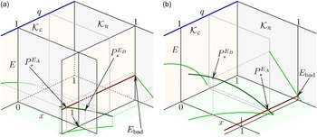


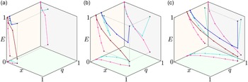


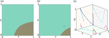


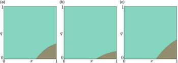


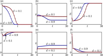


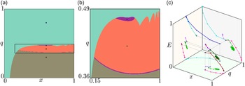


 Open access