


1 INTRODUCTION
The age–metallicity relation (AMR) provides information for our understanding the formation and evolution of the Milky Way. The pioneering studies of Rocha-Pinto et al. (Reference Rocha-Pinto, Maciel, Scalo and Flynn2000) and Twarog (Reference Twarog1980a, Reference Twarogb) show good correlations between age and metallicity. However, recent investigations indicate that the picture is more complicated. As time progresses, the interstellar medium becomes enriched in heavy elements. As a result, newly formed stars should have higher metallicity than the older ones. Contrary to this expectation, we observe metal-rich young and old stars together (e.g. Edvardsson et al. Reference Edvardsson, Andersen, Gustafsson, Lambert, Nissen and Tomkin1993; Carraro Ng, & Portinari Reference Carraro, Ng and Portinari1998; Chen et al. Reference Chen, Nissen, Zhao, Zhang and Benoni2000; Feltzing, Holmberg, & Hurley Reference Feltzing, Holmberg and Hurley2001).
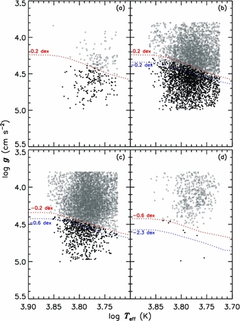
Feltzing et al. (Reference Feltzing, Holmberg and Hurley2001) separated their sample of 5828 dwarf and sub-dwarf stars into five sub-samples in terms of effective temperature; i.e. (a) $3.83<\log T_{\text{eff}}\text{ (K)}$
, (b)
$3.83<\log T_{\text{eff}}\text{ (K)}$
, (b) $3.80< \log T_{\text{eff}}\text{ (K)}\le 3.83$
, (c)
$3.80< \log T_{\text{eff}}\text{ (K)}\le 3.83$
, (c) $3.77<\log T_{\text{eff}}\text{ (K)}\le 3.80$
, (d)
$3.77<\log T_{\text{eff}}\text{ (K)}\le 3.80$
, (d) $3.75<\log T_{\text{eff}}\text{ (K)}\le 3.77$
, and (e)
$3.75<\log T_{\text{eff}}\text{ (K)}\le 3.77$
, and (e) $\log T_{\text{eff}}\text{ (K)}\le 3.75$
. The hottest two sub-samples show a good AMR, but for cooler sub-samples, old metal-rich stars contaminate the expected AMR. Since Feltzing et al. (Reference Feltzing, Holmberg and Hurley2001) derived accurate metallicities from Strömgren photometry, their results are reliable.
$\log T_{\text{eff}}\text{ (K)}\le 3.75$
. The hottest two sub-samples show a good AMR, but for cooler sub-samples, old metal-rich stars contaminate the expected AMR. Since Feltzing et al. (Reference Feltzing, Holmberg and Hurley2001) derived accurate metallicities from Strömgren photometry, their results are reliable.
A similar contamination can be observed in three papers of the Geneva–Copenhagen Survey (GCS) group. The advantage of this group is that their radial velocity data were obtained homogeneously with the photoelectric cross-correlation spectrometers CORAVEL (Baranne, Mayor, & Poncet Reference Baranne, Mayor and Poncet1979; Mayor Reference Mayor, Philip and Latham1985). In the first paper, Nordström et al. (Reference Nordström2004) derived a relation between age and metallicity for young dwarf stars but a substantial scatter in metallicity was present at all ages. They stated that reliable ages cannot be determined for unevolved stars and that the relative errors in individual ages exceed 50%. Such high scattering blurs the expected AMR.
The GCS group improved their calibrations in the following papers. In the second paper, Holmberg, Nordström, & Andersen (Reference Holmberg, Nordström and Andersen2007) included the V − K photometry, whereas in the third paper, Holmberg, Nordström, & Andersen (Reference Holmberg, Nordström and Andersen2009) used the recent revision of Hipparcos parallaxes (van Leeuwen Reference van Leeuwen2007). The most striking feature found in these studies is the existence of metal-rich old stars together with metal-poor old ones, with large scattering.
AMR for Soubiran et al. (Reference Soubiran, Bienaymé, Mishenina and Kovtyukh2008)'s 891 clump giants is different from the one for dwarfs mentioned in the preceding paragraphs. Their results are mainly for the thin disc. The number of metal-rich stars is small in their sample. They derived a vertical metallicity gradient of −0.31 dex kpc−1 and found a transition in metallicity at ~4–5 Gyr. The metallicity decreases with increasing ages up to ~4–5 Gyr, whereas it has a flat distribution at higher ages. Additionally, the metallicity scatter is rather large.
Although the data used for age–metallicity calibrations are improved, we are still far from our aim. Establishing a global relation between age and metallicity is challenging with current data. We deduce from the cited studies that such a relation can be obtained only with some constraints, such as temperature, spectral type, population, and luminosity class. Even under these limitations, the parameters must be derived precisely. Then, we should comment whether the solar neighbourhood is as homogeneous as it was during its formation or whether its evolution has been shaped by mass accretion or spiral waves.
In this paper, we use a different sample of F and G dwarfs and derive the AMR for several sub-samples. The data were taken from RAVE DR3 and are given in Section 2. The main-sequence sample is identified by two constraints, i.e. log g ≥ 3.8 (cm s−2) and $5310 \le T_{\text{eff}} \text{ (K)} \le 7300$
. Parallaxes are not available for stars observed in the RAVE survey. Hence, the distances of the sample stars were calculated by applying the main-sequence colour–luminosity relation of Bilir et al. (Reference Bilir, Karaali, Ak, Yaz, Cabrera-Lavers and Coşkunoğlu2008), which is valid in the absolute magnitude range 0 < MJ
< 6. We de-reddened the colours and magnitudes by using an iterative process and the maps of Schlegel, Finkbeiner, & Davis (Reference Schlegel, Finkbeiner and Davis1998) plus the canonical procedure appearing in the literature (see Section 2.2). We combined the distances, the RAVE kinematics, and the available proper motions to estimate the U, V, W space velocity components which will be used for population analyses. Four types of populations are considered, i.e. high-probability thin disc stars, low-probability thin disc stars, low-probability thick disc stars, and high-probability thick disc stars. The separation of the sample stars into different population categories is carried out by the procedures in Bensby, Feltzing, & Lundström (Reference Bensby, Feltzing and Lundström2003) and Bensby et al. (Reference Bensby, Feltzing, Lundström and Ilyin2005). In Section 3, we used the procedure of Jørgensen & Lindegren (Reference Jørgensen and Lindegren2005), which is based on posterior joint probability for accurate stellar age estimation. AMR for 32 sub-samples is given in Section 4. The sub-samples consist of different spectral and population types and their combination. Section 5 is devoted to summary and discussion.
$5310 \le T_{\text{eff}} \text{ (K)} \le 7300$
. Parallaxes are not available for stars observed in the RAVE survey. Hence, the distances of the sample stars were calculated by applying the main-sequence colour–luminosity relation of Bilir et al. (Reference Bilir, Karaali, Ak, Yaz, Cabrera-Lavers and Coşkunoğlu2008), which is valid in the absolute magnitude range 0 < MJ
< 6. We de-reddened the colours and magnitudes by using an iterative process and the maps of Schlegel, Finkbeiner, & Davis (Reference Schlegel, Finkbeiner and Davis1998) plus the canonical procedure appearing in the literature (see Section 2.2). We combined the distances, the RAVE kinematics, and the available proper motions to estimate the U, V, W space velocity components which will be used for population analyses. Four types of populations are considered, i.e. high-probability thin disc stars, low-probability thin disc stars, low-probability thick disc stars, and high-probability thick disc stars. The separation of the sample stars into different population categories is carried out by the procedures in Bensby, Feltzing, & Lundström (Reference Bensby, Feltzing and Lundström2003) and Bensby et al. (Reference Bensby, Feltzing, Lundström and Ilyin2005). In Section 3, we used the procedure of Jørgensen & Lindegren (Reference Jørgensen and Lindegren2005), which is based on posterior joint probability for accurate stellar age estimation. AMR for 32 sub-samples is given in Section 4. The sub-samples consist of different spectral and population types and their combination. Section 5 is devoted to summary and discussion.
2 DATA
The data used in this study are from RAVE's third data release (DR3; Siebert et al. Reference Siebert2011). RAVE DR3 consists of 82 850 stars, each with equatorial and Galactic coordinates, radial velocity, metallicity, surface temperature, and surface gravity. We also note the two former data releases, i.e. DR1 (Steinmetz et al. Reference Steinmetz2006) and DR2 (Zwitter et al. Reference Zwitter2008). Proper motions were compiled from several catalogues: Tycho-2, Supercosmos Sky Survey, Catalog of Positions and Proper motions on the ICRS (PPMXL; Roeser, Demleitner, & Schilbach Reference Roeser, Demleitner and Schilbach2010), and USNO CCD Astrograph Catalog 2 (UCAC-2). Proper-motion accuracy decreases in this order; therefore, if proper motions were available from all catalogues, Tycho-2's values were used. If Tycho-2 did not provide proper motions, then the values were taken from the Supercosmos Sky Survey, etc. Photometric data are based on the near-IR (NIR) system. The magnitudes of stars were obtained by matching RAVE DR3 with Two Micron All Sky Survey (2MASS; Skrutskie et al. Reference Skrutskie2006) point-source catalogue (Cutri et al. Reference Cutri2003).
2.1 The sample
We applied several constraints to obtain a F- and G-type main-sequence sample from RAVE DR3. First, we selected stars with surface gravities log g(cm s−2) ≥ 3.8 and effective temperatures in the $5310\le T_{\text{eff}} \text{(K)}\le 7300$
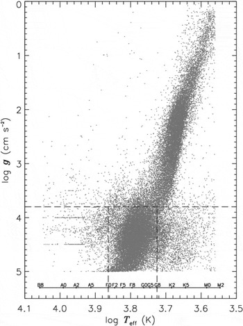
range (Cox Reference Cox and Cox2000). Thus, the sample was reduced to 18 225 stars. The distribution of all DR3 stars in the log g–
$5310\le T_{\text{eff}} \text{(K)}\le 7300$
range (Cox Reference Cox and Cox2000). Thus, the sample was reduced to 18 225 stars. The distribution of all DR3 stars in the log g– $\log T_{\text{eff}}$
plane is given in Figure 1. The F and G main-sequence sample used in this study is also marked in the figure. Then, we separated the star sample into four metallicity intervals, i.e.
$\log T_{\text{eff}}$
plane is given in Figure 1. The F and G main-sequence sample used in this study is also marked in the figure. Then, we separated the star sample into four metallicity intervals, i.e. $0<\text{[M/H]}\le 0.5$
,
$0<\text{[M/H]}\le 0.5$
, $-0.5<\text{[M/H]}\le 0$
,
$-0.5<\text{[M/H]}\le 0$
, $-1.5<\text{[M/H]}\le -0.5$
,
$-1.5<\text{[M/H]}\le -0.5$
, $-2.0<\text{[M/H]}\le -1.5$
dex, and plotted them in the
$-2.0<\text{[M/H]}\le -1.5$
dex, and plotted them in the
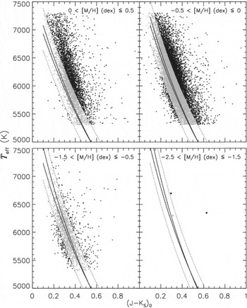
 $T_{\text{eff}}\text{--}(J-K_s)_{0}$
plane (Figure 2) to compare them with the data of González Hernández & Bonifacio (Reference Hernández and Bonifacio2009).
$T_{\text{eff}}\text{--}(J-K_s)_{0}$
plane (Figure 2) to compare them with the data of González Hernández & Bonifacio (Reference Hernández and Bonifacio2009).
Distribution of (all) DR3 stars in the log g– $\log T_{\text{eff}}$
plane. Spectral types are also shown in the horizontal axis.
$\log T_{\text{eff}}$
plane. Spectral types are also shown in the horizontal axis.
The $T_{\text{eff}}$
–(J − Ks
)0 diagram of F and G main-sequence stars in four metallicity intervals. The rigid lines show the region occupied by the stars of González Hernández & Bonifacio (Reference Hernández and Bonifacio2009), while the dotted ones indicate the 2σ dispersion of the mean metallicity in each panel. The rigid line on the left indicates the lower metallicity limit in the corresponding panel, while the right one denotes the higher metallicity limit in the same panel. The two upper panels show that there are differences between the metallicities evaluated in the RAVE DR3 and in González Hernández & Bonifacio (Reference Hernández and Bonifacio2009).
$T_{\text{eff}}$
–(J − Ks
)0 diagram of F and G main-sequence stars in four metallicity intervals. The rigid lines show the region occupied by the stars of González Hernández & Bonifacio (Reference Hernández and Bonifacio2009), while the dotted ones indicate the 2σ dispersion of the mean metallicity in each panel. The rigid line on the left indicates the lower metallicity limit in the corresponding panel, while the right one denotes the higher metallicity limit in the same panel. The two upper panels show that there are differences between the metallicities evaluated in the RAVE DR3 and in González Hernández & Bonifacio (Reference Hernández and Bonifacio2009).
Next, we separated the sample into four metallicity intervals, i.e. $0.2\le \text{[M/H]}$
,
$0.2\le \text{[M/H]}$
, $-0.2\le \text{[M/H]}<0.2$
,
$-0.2\le \text{[M/H]}<0.2$
, $-0.6\le \text{[M/H]}<-0.2$
,
$-0.6\le \text{[M/H]}<-0.2$
, $\text{[M/H]}<-0.6$
dex, and plotted them in the log g–
$\text{[M/H]}<-0.6$
dex, and plotted them in the log g– $\log T_{\text{eff}}$
plane in order to compare their positions with the zero-age-main-sequence (ZAMS) Padova isochrone (Figure 3). The calculation of age by using a set of isochrones for stars with masses
$\log T_{\text{eff}}$
plane in order to compare their positions with the zero-age-main-sequence (ZAMS) Padova isochrone (Figure 3). The calculation of age by using a set of isochrones for stars with masses $0.15<\text{M}_{\odot }\le 100$
, metal abundances 0.0001 ≤ Z ≤ 0.03, and ages from
$0.15<\text{M}_{\odot }\le 100$
, metal abundances 0.0001 ≤ Z ≤ 0.03, and ages from $\log (t/\text{yr})\le 10.13$
is published on the website of the Padova research groupFootnote
1
and described in the work of Marigo et al. (Reference Marigo, Girardi, Bressan, Groenewegen, Silva and Granato2008). We omitted 2669 stars which fall below the ZAMS; thus, the sample was reduced to 8119 stars. Finally, we fitted our stars to the Padova isochrones with ages 0, 2, 4, 6, 8, 10, 12, and 13 Gyr and metallicities
$\log (t/\text{yr})\le 10.13$
is published on the website of the Padova research groupFootnote
1
and described in the work of Marigo et al. (Reference Marigo, Girardi, Bressan, Groenewegen, Silva and Granato2008). We omitted 2669 stars which fall below the ZAMS; thus, the sample was reduced to 8119 stars. Finally, we fitted our stars to the Padova isochrones with ages 0, 2, 4, 6, 8, 10, 12, and 13 Gyr and metallicities $0.2\le \text{[M/H]}$
,
$0.2\le \text{[M/H]}$
, $0\le \text{[M/H]}<0.2$
,
$0\le \text{[M/H]}<0.2$
, $-0.2\le \text{[M/H]}<0$
,
$-0.2\le \text{[M/H]}<0$
, $-0.4\le \text{[M/H]}<-0.2$
,
$-0.4\le \text{[M/H]}<-0.2$
, $-0.6\le \text{[M/H]}<-0.4$
,
$-0.6\le \text{[M/H]}<-0.4$
, $\text{[M/H]}<-0.6$
dex in Figure 4, and excluded the stars not between the isochrones. Thus, we obtained a final sample with 6545 F and G main-sequence stars.
$\text{[M/H]}<-0.6$
dex in Figure 4, and excluded the stars not between the isochrones. Thus, we obtained a final sample with 6545 F and G main-sequence stars.
Position of the star sample in four metallicity intervals, $0.2\le \text{[M/H]}$
,
$0.2\le \text{[M/H]}$
, $-0.2\le \text{[M/H]}<0.2$
,
$-0.2\le \text{[M/H]}<0.2$
, $-0.6\le \text{[M/H]}<-0.2$
,
$-0.6\le \text{[M/H]}<-0.2$
, $\text{[M/H]}<-0.6$
dex, relative to the ZAMS Padova isochrone. Stars which fall below the ZAMS were omitted. The large fraction of stars below the ZAMS are due to the unexpected large values of surface gravity. However, exclusion of these stars do not affect our results, because this scattering is valid for all metallicity intervals.
$\text{[M/H]}<-0.6$
dex, relative to the ZAMS Padova isochrone. Stars which fall below the ZAMS were omitted. The large fraction of stars below the ZAMS are due to the unexpected large values of surface gravity. However, exclusion of these stars do not affect our results, because this scattering is valid for all metallicity intervals.
Star sample in six metallicity intervals fitted to Padova isochrones: (a) $0.2\le \text{[M/H]}$
, (b)
$0.2\le \text{[M/H]}$
, (b) $0\le \text{[M/H]}<0.2$
, (c)
$0\le \text{[M/H]}<0.2$
, (c) $-0.2\le \text{[M/H]}<0$
, (d)
$-0.2\le \text{[M/H]}<0$
, (d) $-0.4\le \text{[M/H]}<-0.2$
, (e)
$-0.4\le \text{[M/H]}<-0.2$
, (e) $-0.6\le \text{[M/H]}<-0.4$
, and (f)
$-0.6\le \text{[M/H]}<-0.4$
, and (f) $\text{[M/H]}<-0.6$
dex.
$\text{[M/H]}<-0.6$
dex.
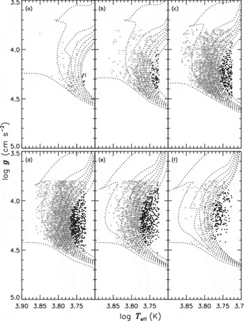
Figure 2 shows that there are substantial differences between the $T_{\text{eff}} \text{--} (J-K_s)_0$
relations for four metallicity intervals of our sample and the one of González Hernández & Bonifacio (Reference Hernández and Bonifacio2009). As the (J − Ks
)0 colours are accurate, the difference in question should originate from the temperatures, i.e. the temperature errors of the sample stars are larger than the mean temperature,
$T_{\text{eff}} \text{--} (J-K_s)_0$
relations for four metallicity intervals of our sample and the one of González Hernández & Bonifacio (Reference Hernández and Bonifacio2009). As the (J − Ks
)0 colours are accurate, the difference in question should originate from the temperatures, i.e. the temperature errors of the sample stars are larger than the mean temperature, $\Delta T \sim 200 \text{K}$
, cited by Siebert et al. (Reference Siebert2011). If we decrease the temperatures of the sample stars such as to fit with the ones of González Hernández & Bonifacio (Reference Hernández and Bonifacio2009), their positions move to lower temperatures as in Figures 3 and 4.
$\Delta T \sim 200 \text{K}$
, cited by Siebert et al. (Reference Siebert2011). If we decrease the temperatures of the sample stars such as to fit with the ones of González Hernández & Bonifacio (Reference Hernández and Bonifacio2009), their positions move to lower temperatures as in Figures 3 and 4.
One can notice a large fraction of stars are below the ZAMS in Figure 3. The surface gravities of these stars extend up to log g = 5.0 (cm s−2), which is not expected. If we decrease the effective temperatures of the sample stars as mentioned in the previous paragraph, the result does not change considerably. Hence, the only explanation of the large fraction of stars in question can be that the errors in surface gravities are (probably) larger than the mean errors cited by Siebert et al. (Reference Siebert2011), i.e. Δlog g = 0.2 (cm s−2). A decrease of Δlog g ~ 0.5 (cm s−2) in the surface gravity moves the sample stars to an agreeable position in Figure 3. Such a revision provides also a much better fitting of the sample stars to the isochrones in Figure 4.
Now, there is a question to be answered: How does such a revision affect the AMR, our main goal in this study? Although a decrease in the effective temperature increases the number of sample stars (Figure 4) not on the isochrones, the reduction of their surface gravities removes them to an agreeable position in the (log g, $\log T_{\text{eff}}$
) plane. Most of the sample stars (if not all) are (thin or thick) disc stars. Moreover, age does not depend on surface gravity. Hence, any revision in temperature or in surface gravity will increase the number of the sample stars at a given position of the AMR but not its trend, i.e. we do not expect any considerable difference in our results if we apply such a revision.
$\log T_{\text{eff}}$
) plane. Most of the sample stars (if not all) are (thin or thick) disc stars. Moreover, age does not depend on surface gravity. Hence, any revision in temperature or in surface gravity will increase the number of the sample stars at a given position of the AMR but not its trend, i.e. we do not expect any considerable difference in our results if we apply such a revision.
2.2 Distance determination
Contrary to the Hipparcos catalogue (ESA 1997), parallaxes are not available for stars observed in the RAVE survey (Steinmetz et al. Reference Steinmetz2006). Hence, the distances of the sample stars were calculated using another procedure. We applied the main-sequence colour–luminosity relation of Bilir et al. (Reference Bilir, Karaali, Ak, Yaz, Cabrera-Lavers and Coşkunoğlu2008), which is valid in the 0 < MJ < 6 range, where MJ is the absolute magnitude in the J band of 2MASS photometry. The errors of the distances were estimated combining the internal errors of the coefficients of Bilir et al. (Reference Bilir, Karaali, Ak, Yaz, Cabrera-Lavers and Coşkunoğlu2008)'s equation and the errors of the 2MASS colour indices.
As most of the stars in the sample are at distances larger than 100 pc, their colours and magnitudes are affected by interstellar reddening. Hence, distance determination is carried out simultaneously by the de-reddening of the sample stars. As a first step in an iterative process, we assume the original (J − H) and (H − Ks ) colour indices are de-reddened, and evaluate the MJ absolute magnitude of the sample stars by means of the colour–luminosity relation of Bilir et al. (Reference Bilir, Karaali, Ak, Yaz, Cabrera-Lavers and Coşkunoğlu2008). A combination of the apparent and absolute magnitudes for the J band gives the distance of a star. We used the maps of Schlegel et al. (Reference Schlegel, Finkbeiner and Davis1998) and evaluated the colour excess E(B − V) for each sample star. The relation between the total and selective absorptions in the UBV system, i.e.
 \begin{equation}
A_{\infty }(b)=3.1\times E_{\infty }(B-V)
\end{equation}
\begin{equation}
A_{\infty }(b)=3.1\times E_{\infty }(B-V)
\end{equation}
 \begin{equation}
A_{d}(b)=A_{\infty }(b)\times \Biggl [1-\exp \Biggl (\frac{-\mid d \sin (b)\mid }{H}\Biggr )\Biggr ],
\end{equation}
\begin{equation}
A_{d}(b)=A_{\infty }(b)\times \Biggl [1-\exp \Biggl (\frac{-\mid d \sin (b)\mid }{H}\Biggr )\Biggr ],
\end{equation}
 \begin{equation}
A_{d}(b)=3.1\times E_{d}(B-V).
\end{equation}
\begin{equation}
A_{d}(b)=3.1\times E_{d}(B-V).
\end{equation}
The reduced colour excess was used in Fiorucci & Munari's (2003) equations to obtain the total absorptions for the J, H, and Ks bands, i.e. AJ = 0.887 × E(B − V), AH = 0.565 × E(B − V), and AKs = 0.382 × E(B − V), which were used in Pogson's equation (mi − Mi = 5 log d − 5 + Ai ; i denotes a specific band) to estimate distances. Contrary to the assumption above, the original (J − H) and (H − Ks ) colour indices are not de-reddened. Hence, the application of equations (1) to (3) is iterated until the distance d and the colour index Ed (B − V) approach constant values.
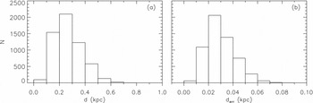
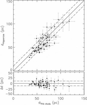
The distribution of the distances (Figure 5) shows that ~80% of the sample stars have almost a normal distribution within the distance interval 0 < d ≤ 0.4 kpc, whereas the overall distribution, which extends up to 1 kpc, is skewed, with a median of 0.25 kpc. However, ~99% the sample stars are within d = 0.6 kpc. We compared the distances for a set of stars estimated in our study with those evaluated by their parallaxes to test our distances, as explained in the following. There are 51 main-sequence stars with small relative parallax errors, σπ/π ≤ 0.20, common in RAVE DR3 and the newly reduced Hipparcos catalogue (van Leeuwen Reference van Leeuwen2007) for which one can evaluate accurate distances. The constraints applied for providing this sample are as follows: MV >4, log g>3.80 (cm s−2) and σπ/π ≤ 0.20. Figure 6 shows that there is a good agreement between two sets of distances. The mean and the standard deviations of the residuals are 0 and 11 pc, respectively. The number of stars common in the Hipparcos catalogue and in RAVE DR3 decreases, while their scatter grows with distance becoming 25% of the distance at 100 pc. The parallaxes in the Hipparcos catalogue are not available to estimate the scatter at larger distances such as 600 pc, the largest distance reported in our study.
Frequency (a) and error (b) distributions of distances of F–G main-sequence stars.
Comparison of the distances estimated in our work with those evaluated by means of their parallaxes taken from the Hipparcos catalogue. The one-to-one line is also given in the figure.
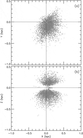
The positions of the sample stars in the rectangular coordinate system relative to the Sun are given in Figure 7. The projected shapes both on the Galactic (X, Y) plane and the vertical (X, Z) plane of the sample show asymmetrical distributions. The median coordinates (X = 61, Y = −97, Z = −114 pc) of the sample stars confirm this appearance. The inhomogeneous structure is due to the incomplete observations of the RAVE project and that the program stars were selected from the Southern Galactic hemisphere (Steinmetz et al. Reference Steinmetz2006).
Space distributions of RAVE DR3 F–G main-sequence stars on two planes: (a) X − Y and (b) X − Z.
2.3 Kinematics
We combined the distances estimated in Section 2.2 with RAVE kinematics and available proper motions, applying the algorithms and the transformation matrices of Johnson & Soderblom (Reference Johnson and Soderblom1987) to obtain their Galactic space velocity components (U, V, W). In the calculations, the epoch of J2000 was adopted as described in the International Celestial Reference System (ICRS) of the Hipparcos and Tycho-2 Catalogues (ESA 1997). The transformation matrices use the notation of a right-handed system. Hence, U, V, and W are the components of a velocity vector of a star with respect to the Sun, where U is positive towards the Galactic centre (l = 0°, b = 0°), V is positive in the direction of Galactic rotation (l = 90°, b = 0°), and W is positive towards the North Galactic Pole (b = 90°).
Correction for differential Galactic rotation is necessary for an accurate determination of the U, V, and W velocity components. The effect is proportional to the projection of the distance to the stars onto the Galactic plane, i.e. the W velocity component is not affected by Galactic differential rotation (Mihalas & Binney Reference Mihalas and Binney1981). We applied the procedure of Mihalas & Binney (Reference Mihalas and Binney1981) to the distribution of the sample stars in the X–Y plane and estimated the first-order Galactic differential rotation corrections for the U and V velocity components of the sample stars. The range of these corrections is $-25.4<\text{d}U<11$
and
$-25.4<\text{d}U<11$
and $-2.1<\text{d}V<1.6$
km s−1 for U and V, respectively. As expected, U is affected more than the V component. Also, the high values for the U component show that corrections for differential Galactic rotation cannot be ignored.
$-2.1<\text{d}V<1.6$
km s−1 for U and V, respectively. As expected, U is affected more than the V component. Also, the high values for the U component show that corrections for differential Galactic rotation cannot be ignored.
The uncertainty of the space velocity components $U_{\text{err}}$
,
$U_{\text{err}}$
, $V_{\text{err}}$
, and
$V_{\text{err}}$
, and $W_{\text{err}}$
was computed by propagating the uncertainties of the proper motions, distances, and radial velocities, again using an algorithm by Johnson & Soderblom (Reference Johnson and Soderblom1987). Then, the error for the total space velocity of a star follows from the equation:
$W_{\text{err}}$
was computed by propagating the uncertainties of the proper motions, distances, and radial velocities, again using an algorithm by Johnson & Soderblom (Reference Johnson and Soderblom1987). Then, the error for the total space velocity of a star follows from the equation:
 \begin{equation}
S_{\rm err}^{2}=U_{\rm err}^{2}+V_{\rm err}^{2}+W_{\rm err}^{2}.
\end{equation}
\begin{equation}
S_{\rm err}^{2}=U_{\rm err}^{2}+V_{\rm err}^{2}+W_{\rm err}^{2}.
\end{equation}
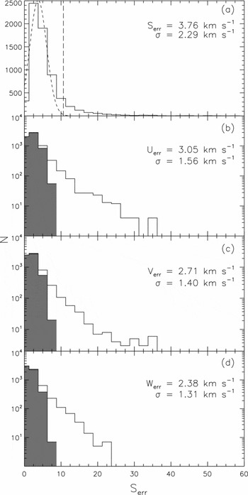
The distributions of errors for both the total space velocity and its components are plotted in Figure 8. The median and standard deviation for space velocity errors are $\tilde{S}_{\rm err}=3.76$
km s−1 and s = 2.29 km s−1, respectively. We now remove the most discrepant data from the analysis, knowing that outliers in a survey such as this will preferentially include stars which are systematically mis-analysed binaries, etc. Thus, we omit stars with errors that deviate by more than the sum of the standard error and three times of the standard deviation, i.e. S
err>10.63 km s−1. This removes 854 stars, 13% of the sample. Thus, our sample was reduced to 5691 stars, those with more robust space velocity components. After applying this constraint, the median values and the standard deviations for the velocity components were reduced to (
$\tilde{S}_{\rm err}=3.76$
km s−1 and s = 2.29 km s−1, respectively. We now remove the most discrepant data from the analysis, knowing that outliers in a survey such as this will preferentially include stars which are systematically mis-analysed binaries, etc. Thus, we omit stars with errors that deviate by more than the sum of the standard error and three times of the standard deviation, i.e. S
err>10.63 km s−1. This removes 854 stars, 13% of the sample. Thus, our sample was reduced to 5691 stars, those with more robust space velocity components. After applying this constraint, the median values and the standard deviations for the velocity components were reduced to ( $\tilde{U}_{\rm err}, \tilde{V}_{\rm err}, \tilde{W}_{\rm err})=(3.05\pm 1.56, 2.71\pm 1.40, 2.38\pm 1.31)$
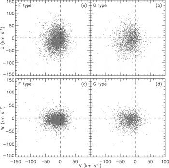
km s−1. The two-dimensional distribution of the velocity components for the reduced sample is given in Figure 9.
$\tilde{U}_{\rm err}, \tilde{V}_{\rm err}, \tilde{W}_{\rm err})=(3.05\pm 1.56, 2.71\pm 1.40, 2.38\pm 1.31)$
km s−1. The two-dimensional distribution of the velocity components for the reduced sample is given in Figure 9.
Error histograms for space velocity (a) and its components (b–d) for RAVE DR3 F–G main-sequence stars. The vertical dashed line in panel (a) indicates the upper limit of the total error adopted in this work. The shaded part of the histogram indicates the error for different velocity components of stars after removing the stars with large space velocity errors.
The distribution of velocity components of our final sample of RAVE DR3 F–G main-sequence stars with high-quality data, in two projections: U − V (a and c) and W − V (b and d).
2.4 Population analysis
We now wish to consider the population kinematics as a function of stellar population, using space motion as a statistical process to label stars as members of a stellar population. We used the procedure of Bensby et al. (Reference Bensby, Feltzing and Lundström2003, Reference Bensby, Feltzing, Lundström and Ilyin2005) to allocate the main-sequence sample (5691 stars) into populations and derived the solar space velocity components for the thin disc population to check the dependence of Local Standard of Rest (LSR) parameters on population. Bensby et al. (Reference Bensby, Feltzing and Lundström2003, Reference Bensby, Feltzing, Lundström and Ilyin2005) assumed that the Galactic space velocities of stellar populations with respect to the LSR have Gaussian distributions as follows:
 \begin{equation}
f(U, V, W)=k \times \exp \Biggl (-\frac{U_{\rm LSR}^{2}}{2\sigma _{U{_{\rm LSR}}}^{2}}-\frac{(V_{\rm LSR}-V_{\rm asym}) ^{2}}{2\sigma _{V{_{\rm LSR}}}^{2}}-\frac{W_{\rm LSR}^{2}}{2\sigma _{W{_{\rm LSR}}}^{2}}\Biggr ),
\end{equation}
\begin{equation}
f(U, V, W)=k \times \exp \Biggl (-\frac{U_{\rm LSR}^{2}}{2\sigma _{U{_{\rm LSR}}}^{2}}-\frac{(V_{\rm LSR}-V_{\rm asym}) ^{2}}{2\sigma _{V{_{\rm LSR}}}^{2}}-\frac{W_{\rm LSR}^{2}}{2\sigma _{W{_{\rm LSR}}}^{2}}\Biggr ),
\end{equation}
 \begin{equation}
k=\frac{1}{(2\pi )^{3/2}\sigma _{U{_{\rm LSR}}}\sigma _{V{_{\rm LSR}}}\sigma _{W{_{\rm LSR}}}}
\end{equation}
\begin{equation}
k=\frac{1}{(2\pi )^{3/2}\sigma _{U{_{\rm LSR}}}\sigma _{V{_{\rm LSR}}}\sigma _{W{_{\rm LSR}}}}
\end{equation}
normalises the expression. For consistency with other analyses, we adopt σ U LSR , σ V LSR , and σ W LSR as the characteristic velocity dispersions: 35, 20, and 16 km s−1 for thin disc (D); 67, 38, and 35 km s−1 for thick disc (TD); 160, 90, and 90 km s−1 for halo (H), respectively (Bensby et al. Reference Bensby, Feltzing and Lundström2003). V asym is the asymmetric drift: −15, −46, and −220 km s−1 for thin disc, thick disc, and halo, respectively. U LSR, V LSR, and W LSR are LSR velocities. The space velocity components of the sample stars relative to the LSR were estimated by adding the values for the space velocity components to the corresponding solar ones evaluated by Coşkunoğlu et al. (Reference Coşkunoğlu2011).
The probability of a star of being ‘a member’ of a given population is defined as the ratio of the f (U, V, W) distribution functions times the ratio of the local space densities for two populations. Thus,
 \begin{equation}
TD/D=\frac{X_{TD}}{X_{D}}\times \frac{f_{TD}}{f_{D}}\quad \ \text{and}\quad TD/H=\frac{X_{TD}}{X_{H}}\times \frac{f_{TD}}{f_{H}}
\end{equation}
\begin{equation}
TD/D=\frac{X_{TD}}{X_{D}}\times \frac{f_{TD}}{f_{D}}\quad \ \text{and}\quad TD/H=\frac{X_{TD}}{X_{H}}\times \frac{f_{TD}}{f_{H}}
\end{equation}
Distribution of the sample stars for different stellar population categories.
U − V and W − V diagrams of F- and G-type stars applying Bensby et al.'s (Reference Bensby, Feltzing and Lundström2003) population classification criteria. It is seen that space–motion uncertainties remain significant, even for this nearby sample.
3 STELLAR AGE ESTIMATION
We used the procedure of Jørgensen & Lindegren (Reference Jørgensen and Lindegren2005) for stellar age estimation. We give a small description of the procedure in this study. We quote Jørgensen & Lindegren (Reference Jørgensen and Lindegren2005)'s paper for details. This procedure is based on the so-called (posterior) joint probability density function (pdf) as defined in the following:
 \begin{equation}
f(\tau ,\zeta ,m) \propto f_0(\tau ,\zeta ,m)\, L(\tau ,\zeta ,m),
\end{equation}
\begin{equation}
f(\tau ,\zeta ,m) \propto f_0(\tau ,\zeta ,m)\, L(\tau ,\zeta ,m),
\end{equation}
The likelihood function (L) equals the probability of getting the observed data q( $\log T_{\text{eff}}$
, log g,
$\log T_{\text{eff}}$
, log g, $\text{[M/H]}$
) for given parameters p(τ, ζ, m). Then, the likelihood function is
$\text{[M/H]}$
) for given parameters p(τ, ζ, m). Then, the likelihood function is
 \begin{equation}
L(\tau ,\zeta ,m) = \left( \prod _{i=1}^n \frac{1}{(2\pi )^{1/2}\sigma _i} \right) \times \exp (-\chi ^2/2),
\end{equation}
\begin{equation}
L(\tau ,\zeta ,m) = \left( \prod _{i=1}^n \frac{1}{(2\pi )^{1/2}\sigma _i} \right) \times \exp (-\chi ^2/2),
\end{equation}
 \begin{equation}
\chi ^2 = \sum _{i=1}^n \left(\frac{q_i^{\rm obs}-q_i(\tau ,\zeta ,m)}{\sigma _i}\right)^2,
\end{equation}
\begin{equation}
\chi ^2 = \sum _{i=1}^n \left(\frac{q_i^{\rm obs}-q_i(\tau ,\zeta ,m)}{\sigma _i}\right)^2,
\end{equation}
The prior density of the model parameters in equation (8) can be written as
 \begin{equation}
f_0(\tau ,\zeta ,m) = \psi (\tau )\phi (\zeta \vert \tau )\xi (m\vert \zeta ,\tau ),
\end{equation}
\begin{equation}
f_0(\tau ,\zeta ,m) = \psi (\tau )\phi (\zeta \vert \tau )\xi (m\vert \zeta ,\tau ),
\end{equation}
Following Jørgensen & Lindegren (Reference Jørgensen and Lindegren2005), we adopted the metallicity distribution as a flat function and a power law
 \begin{equation}
\xi (m) \propto m^{-\alpha },
\end{equation}
\begin{equation}
\xi (m) \propto m^{-\alpha },
\end{equation}
 \begin{equation}
f(\tau ) \propto \psi (\tau )G(\tau ),
\end{equation}
\begin{equation}
f(\tau ) \propto \psi (\tau )G(\tau ),
\end{equation}
 \begin{equation}
G(\tau ) \propto \int \!\int L(\tau ,\zeta ,m)\xi (m)\, \mbox{d}m\, \mbox{d}\zeta .
\end{equation}
\begin{equation}
G(\tau ) \propto \int \!\int L(\tau ,\zeta ,m)\xi (m)\, \mbox{d}m\, \mbox{d}\zeta .
\end{equation}
We normalise equation (14) such that G(τ) = 1 at its maximum. Jørgensen & Lindegren (Reference Jørgensen and Lindegren2005) interpreted G(τ) as the relative likelihood of τ after eliminating m and ζ.
Following Jørgensen & Lindegren (Reference Jørgensen and Lindegren2005), we evaluated equation (14) for each age value (τ
i
) as a double sum along a set of isochrones at the required age that are equidistant in metallicity (ζ
k
). In practice, we used pre-computed isochrones for a step size of 0.05 dex in ζ and considered only those within $\pm 3.5\sigma _{\text{[M/H]}}$
of the observed metallicity. Let mjkl
be the initial-mass values along each isochrone (τ
j
, ζ
k
); then
$\pm 3.5\sigma _{\text{[M/H]}}$
of the observed metallicity. Let mjkl
be the initial-mass values along each isochrone (τ
j
, ζ
k
); then
 \begin{equation}
G(\tau _j) \propto \sum _k \sum _\ell L(\tau _j,\zeta _k,m_{jk\ell }) \xi (m_{jk\ell })(m_{jk\ell +1}-m_{jk\ell -1}).
\end{equation}
\begin{equation}
G(\tau _j) \propto \sum _k \sum _\ell L(\tau _j,\zeta _k,m_{jk\ell }) \xi (m_{jk\ell })(m_{jk\ell +1}-m_{jk\ell -1}).
\end{equation}
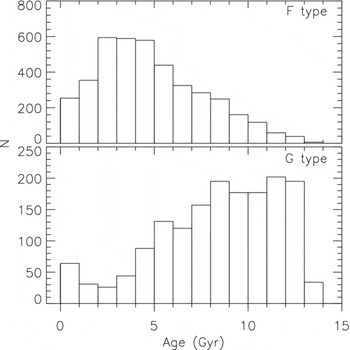
Age corresponding to the mode of the relative posterior probability G(τ) is adopted as the age of the star in question. The distribution of the ages for the final sample (5691 stars) is given in Figure 11.
Age distribution of the RAVE DR3 F and G main-sequence stars.
We tested the ages estimated in this study by comparing them with those estimated in the GCS by using the procedure explained in the following. RAVE and GCS surveys have 142 stars in common. The $T_{\text{eff}}$
, MV
, and
$T_{\text{eff}}$
, MV
, and $\text{[M/H]}$
parameters of 66 stars in this sample were determined by Holmberg et al. (Reference Holmberg, Nordström and Andersen2009). As we considered only the main-sequence stars, we applied the constraint MV
>4. Thus, the sample reduced to 25 stars. We estimated the ages of these stars by using PARAMFootnote
2
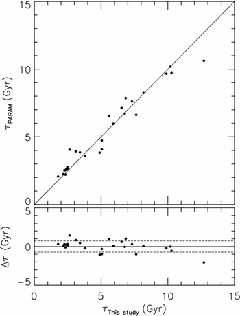
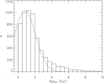
webpage and compared them with the ages estimated by the procedure in our study. The results are given in Figure 12. Although the final sample consists of a limited number of stars, there is a good agreement between the two sets of ages. The errors for all the stars in our study are fitted to a Gaussian distribution in Figure 13. The mode and the standard deviation of the distribution are 0.81 and 1.25 Gyr, respectively. The ages as well as other stellar parameters of the final sample can be provided from Table 2, which is given electronically.
$\text{[M/H]}$
parameters of 66 stars in this sample were determined by Holmberg et al. (Reference Holmberg, Nordström and Andersen2009). As we considered only the main-sequence stars, we applied the constraint MV
>4. Thus, the sample reduced to 25 stars. We estimated the ages of these stars by using PARAMFootnote
2
webpage and compared them with the ages estimated by the procedure in our study. The results are given in Figure 12. Although the final sample consists of a limited number of stars, there is a good agreement between the two sets of ages. The errors for all the stars in our study are fitted to a Gaussian distribution in Figure 13. The mode and the standard deviation of the distribution are 0.81 and 1.25 Gyr, respectively. The ages as well as other stellar parameters of the final sample can be provided from Table 2, which is given electronically.
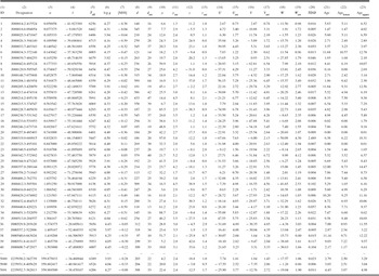
Stellar atmospheric parameters, astrometric, kinematic, and age data for the whole sample: (1) Our catalogue number, (2) RAVEID, (3–4) equatorial coordinates in degrees (J2000), (5) $T_{\textrm {eff}}$
in K, (6) log g (cm s−2) in dex, (7) calibrated metallicity
$T_{\textrm {eff}}$
in K, (6) log g (cm s−2) in dex, (7) calibrated metallicity $\text{[M/H]}$
(dex), (8–9) d distance and its error (pc), (10–11) total proper motion and its error in (mas yr−1), (12–13) heliocentric radial velocity and its error in km s−1, (14–19) Galactic space velocity components, and their respective errors in km s−1, (20) TD/D ratio as mentioned in the text, (21–23) age and its lower and upper confidential levels.
$\text{[M/H]}$
(dex), (8–9) d distance and its error (pc), (10–11) total proper motion and its error in (mas yr−1), (12–13) heliocentric radial velocity and its error in km s−1, (14–19) Galactic space velocity components, and their respective errors in km s−1, (20) TD/D ratio as mentioned in the text, (21–23) age and its lower and upper confidential levels.
Comparison of the ages for 25 stars estimated in our study with the ones evaluated by applying the PARAM webpage to the data $T_{\text{eff}}$
, MV
, and
$T_{\text{eff}}$
, MV
, and $\text{[M/H]}$
taken from Holmberg et al. (Reference Holmberg, Nordström and Andersen2009). The dashed lines indicate ± 1σ limits.
$\text{[M/H]}$
taken from Holmberg et al. (Reference Holmberg, Nordström and Andersen2009). The dashed lines indicate ± 1σ limits.
Distribution of errors for ages estimated in our study. The dashed curve indicates the Gaussian distribution.
4 AGE–METALLICITY RELATION
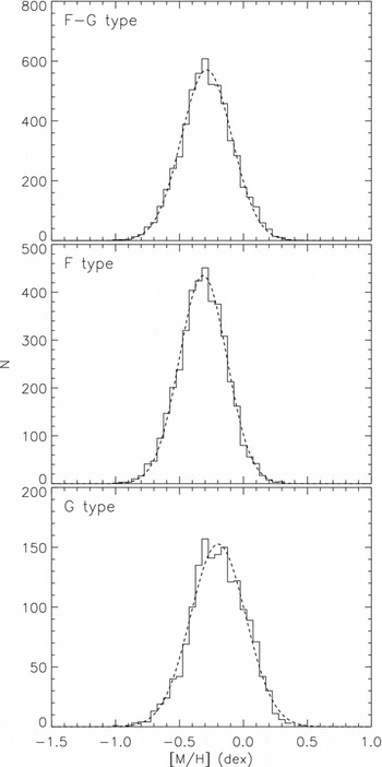
In this section, we investigate the AMR. The distribution of metallicities for our sample is given in Figure 14 as a function of spectral type. The distributions for F and G spectral types and their combination give the indication of a Gaussian distribution with slightly different modes, i.e. ~ −0.31, ~ −0.20, and ~ −0.29 dex for F and G types, and their combination. F stars are intrinsically brighter than G stars, so sample larger distances and thus include a higher proportion of thick disc stars, which shifts the $\text{[M/H]}$
distribution to metal-poor regions. The normalised metallicity distribution for both spectral types shows an expected slight shift of the mode as a function of population (Figure 15). This shows that RAVE DR3 metallicities are approximately correct. However, Figure 26 of Nordström et al. (Reference Nordström2004) shows that the RAVE DR3 distribution appears to be missing a metal-poor tail that should make the metallicity distribution more asymmetric. RAVE DR3
$\text{[M/H]}$
distribution to metal-poor regions. The normalised metallicity distribution for both spectral types shows an expected slight shift of the mode as a function of population (Figure 15). This shows that RAVE DR3 metallicities are approximately correct. However, Figure 26 of Nordström et al. (Reference Nordström2004) shows that the RAVE DR3 distribution appears to be missing a metal-poor tail that should make the metallicity distribution more asymmetric. RAVE DR3 $\text{[M/H]}$
metallicities have an improved calibration compared to RAVE DR2, but this shows that it still needs to be calibrated robustly to a
$\text{[M/H]}$
metallicities have an improved calibration compared to RAVE DR2, but this shows that it still needs to be calibrated robustly to a $[\text{Fe/H}]$
metallicity scale. Given these metal-poor stars are a minority, a minority of individual stellar ages derived from these incorrectly derived metallicities will also be incorrect. Nevertheless, the majority of metallicities and ages will be approximately correct, which is adequate for our goal of investigating general statistical trends in the AMR.
$[\text{Fe/H}]$
metallicity scale. Given these metal-poor stars are a minority, a minority of individual stellar ages derived from these incorrectly derived metallicities will also be incorrect. Nevertheless, the majority of metallicities and ages will be approximately correct, which is adequate for our goal of investigating general statistical trends in the AMR.
Distribution of metallicities of the star sample as a function of spectral type, fitted to a Gaussian distribution.
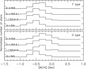
Normalised metallicity distributions for different populations of F- and G-type main-sequence stars.
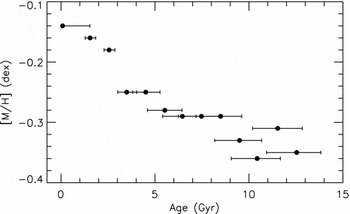
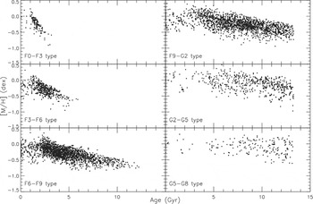
The metallicity distribution of all sample stars in terms of age in Figure 16 reminds us the complicated picture claimed in Section 1: there are metal-rich old stars in addition to the young ones. Figure 16 is qualitatively similar to Nordström et al. (Reference Nordström2004)'s Figure 27. We separated our sample into six sub-samples, i.e. F0–F3, F3–F6, F6–F9, F9–G2, G2–G5, and G5–G8, and investigated the AMR for each sub-sample (Figure 17). The most conspicuous feature in Figure 17 is the absence of old metal-rich stars in the relatively early spectral types. These stars appear in the F9–G2 spectral types and dominate later spectral types. The second feature in the distributions in Figure 17 is the slope which decreases (absolutely) gradually when one goes from sub-sample F0–F3 to the sub-samples including stars from later spectral types and becomes almost zero for the sub-sample G5–G8. Finally, the third feature in Figure 17 is the different range of the age, i.e. 0 < t ≤ 3, t ≤ 6, and t ≤ 13 Gyr, for F0–F3, F3–F6, and F6–G8 spectral types, respectively. Additionally, the number of old stars increases for later spectra types, as expected.
Age–metallicity distribution of (all) sample stars.
Age–metallicity relation as a function of spectral type as indicated in six panels.
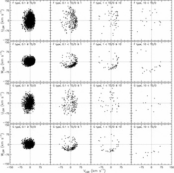
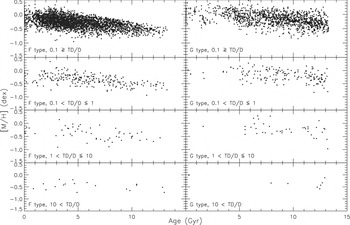
We investigated the relation between age and metallicity also as a function of population, i.e. TD/D ≤ 0.1, 0.1 < TD/D ≤ 1, 1 < TD/D ≤ 10, and 10 < TD/D. The distributions are given in Figure 18 for F and G types individually. One can notice similar metallicity distributions for F- and G-type stars. Small slopes are apparent, with the exception of F-type stars with TD/D>10, i.e. high-probability thick disc stars, for which the distribution is flat. As in Figure 17, the majority of the old, metal-rich stars are of G spectral type.
Age-metallicity distribution as a function of population for F and G type stars as indicated in eight panels.
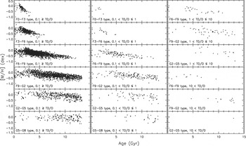
We applied both constraints stated above and plotted the metallicity of the sample stars versus their age. Thus, AMR for F0–F3, F3–F6, F6–F9, F9–G2, G2–G5, and G5–G8 sub-samples are now plotted for the population types TD/D ≤ 0.1, 0.1 < TD/D ≤ 1, 1 < TD/D ≤ 10 (Figure 19). A comparison of the distributions in Figures 18 and 19 shows that population is not a strong indicator for an AMR, whereas, metallicity–age distribution for a series of narrow spectral-type intervals shows a slope.
Age-mentallicity relations as a function of both spectral type and population as indicated in 18 panels.
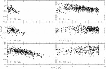
In Section 2, we mentioned the errors of the effective temperatures and the surface gravities of the stars. We investigated their effects on our final results, i.e. the AMR, by using the procedure explained in the following. We used the metallicity of a sample star and estimated its surface gravity, effective temperature, and age simultaneously by means of the Padova isochrones. We called it ‘artificial age’. A second age has been determined using the metallicity, surface gravity, and effective temperature in question plus the corresponding mean errors stated for the RAVE DR3 survey. The second set of ages, called ‘RAVE ages’, was estimated by the procedure of Jørgensen & Lindegren (Reference Jørgensen and Lindegren2005) as explained in Section 3. We obtained AMR for two sets of ages for 32 sub-samples and evaluated the differences between two ages (the residuals) for a given metallicity for each sub-sample. We plotted only six of the AMR for the ‘artificial ages’, i.e. those for the spectral types F0–F3, F3–F6, F6–F9, F9–G2, G2–G5, and G5–G8, in Figure 20 just as an example, but we evaluated the mean and standard deviations for the residuals of all sub-samples. Table 3 shows that the mean residuals and the corresponding standard deviations are smaller for the F-type stars than for the G-type ones.
“Artificial” age-metallicity relation as a function of spectral type as indicated in six panels.
Mean and standard deviations for the differences between the ages estimated by means of two different sets of data for different spectral type intervals and for different population types (statistics for the combination of the spectral types and population types, not given in this table, are not different than the ones for corresponding spectral types). The last column gives 25% of the mean age for comparison the errors in this study with those in the literature (see the text).
Jørgensen & Lindegren (Reference Jørgensen and Lindegren2005) stated that the errors of the stellar ages in their study are at least 25% of the corresponding age. A similar result can be found in Nordström et al. (Reference Nordström2004), i.e. the stellar age errors of 9428 stars in their study are less than 50% of their ages while those for 5472 stars are less than 25%. We evaluated 25% of the mean age for each sub-sample in Table 3 (last column) and compared them with the (absolute) sum of the corresponding mean age residuals, $\langle \Delta \text{Age}\rangle$
and standard deviations, σ. The sum of two statistics is less than 25% of the mean age for all sub-samples, except the sub-sample G5–G8. Thus, we can say that the estimated ages and the AMR are confident.
$\langle \Delta \text{Age}\rangle$
and standard deviations, σ. The sum of two statistics is less than 25% of the mean age for all sub-samples, except the sub-sample G5–G8. Thus, we can say that the estimated ages and the AMR are confident.
5 SUMMARY AND DISCUSSION
We applied the following constraints to the RAVE DR3 data consisting of 82 850 stars and obtained the AMR for 5691 F and G spectral-type stars: (i) We selected stars with surface gravities log g (cm s−2) ≥ 3.8 and effective temperatures $5310\le T_{\text{eff}} {\rm (K)}\le 7300$
. These are the surface gravity range of the main-sequence stars and the temperature range of F- and G-type stars, respectively. (ii) We separated the stars into the metallicity intervals
$5310\le T_{\text{eff}} {\rm (K)}\le 7300$
. These are the surface gravity range of the main-sequence stars and the temperature range of F- and G-type stars, respectively. (ii) We separated the stars into the metallicity intervals $0<\text{[M/H]}\le 0.5$
,
$0<\text{[M/H]}\le 0.5$
, $-0.5<\text{[M/H]}\le 0$
,
$-0.5<\text{[M/H]}\le 0$
, $-1.5<\text{[M/H]}\le -0.5$
,
$-1.5<\text{[M/H]}\le -0.5$
, $-2<\text{[M/H]}\le -1.5$
dex, and plotted them in the
$-2<\text{[M/H]}\le -1.5$
dex, and plotted them in the $T_{\text{eff}}$
–(J − Ks
)0 plane compared to the data of González Hernández & Bonifacio (Reference Hernández and Bonifacio2009). Then, we omitted stars which did not fit the temperature–colour plane of González Hernández & Bonifacio (Reference Hernández and Bonifacio2009). (iii) We separated the remaining stars into
$T_{\text{eff}}$
–(J − Ks
)0 plane compared to the data of González Hernández & Bonifacio (Reference Hernández and Bonifacio2009). Then, we omitted stars which did not fit the temperature–colour plane of González Hernández & Bonifacio (Reference Hernández and Bonifacio2009). (iii) We separated the remaining stars into $0.2\le \text{[M/H]}$
,
$0.2\le \text{[M/H]}$
, $-0.2\le \text{[M/H]}<0.2$
,
$-0.2\le \text{[M/H]}<0.2$
, $-0.6\le \text{[M/H]}<-0.2$
,
$-0.6\le \text{[M/H]}<-0.2$
, $\text{[M/H]}<-0.6$
dex metallicity intervals and plotted them in the log g–
$\text{[M/H]}<-0.6$
dex metallicity intervals and plotted them in the log g– $\log T_{\text{eff}}$
plane in order to compare their positions with the ZAMS of Padova isochrones. We omitted the stars which fell below the ZAMS. (iv) We fitted the remaining stars to the Padova ischrones with ages 0, 2, 4, 6, 8, 10, 12, and 13 Gyr and metallicities
$\log T_{\text{eff}}$
plane in order to compare their positions with the ZAMS of Padova isochrones. We omitted the stars which fell below the ZAMS. (iv) We fitted the remaining stars to the Padova ischrones with ages 0, 2, 4, 6, 8, 10, 12, and 13 Gyr and metallicities $0.2\le \text{[M/H]}$
,
$0.2\le \text{[M/H]}$
, $0\le \text{[M/H]}<0.2$
,
$0\le \text{[M/H]}<0.2$
, $-0.2\le \text{[M/H]}<0$
,
$-0.2\le \text{[M/H]}<0$
, $-0.4\le \text{[M/H]}<-0.2$
,
$-0.4\le \text{[M/H]}<-0.2$
, $-0.6\le \text{[M/H]}<-0.4$
,
$-0.6\le \text{[M/H]}<-0.4$
, $\text{[M/H]}<-0.6$
dex, and excluded the stars with positions beyond the log g–
$\text{[M/H]}<-0.6$
dex, and excluded the stars with positions beyond the log g– $\log T_{\emph {eff}}$
plane occupied by the isochrones from the sample. (v) Finally, we omitted the stars with total velocity error S
err>10.63 km s−1. After these constraints, the sample was reduced to 5691 F- and G-type main-sequence stars.
$\log T_{\emph {eff}}$
plane occupied by the isochrones from the sample. (v) Finally, we omitted the stars with total velocity error S
err>10.63 km s−1. After these constraints, the sample was reduced to 5691 F- and G-type main-sequence stars.
The distances of the sample stars were determined by the colour–luminosity relation of Bilir et al. (Reference Bilir, Karaali, Ak, Yaz, Cabrera-Lavers and Coşkunoğlu2008), and the J, H, and Ks magnitudes were de-reddened by the procedure in situ and the equations of Fiorucci & Munari (Reference Fiorucci and Munari2003). We combined the distances with RAVE kinematics and available proper motions, applying the algorithms and the transformation matrices of Johnson & Soderblom (Reference Johnson and Soderblom1987) to obtain the Galactic space velocity components (U, V, W). We used the procedure of Bensby et al. (Reference Bensby, Feltzing and Lundström2003, Reference Bensby, Feltzing, Lundström and Ilyin2005) to divide the main-sequence sample (5691 stars) into populations and derived the solar space velocity components for the thin and thick discs and halo populations to check the AMR on population. We used the Bayesian procedure of Jørgensen & Lindegren (Reference Jørgensen and Lindegren2005) to estimate stellar ages. This procedure is based on the joint pdf, which consists of a prior probability density of the parameters and a likelihood function, and which claims stellar ages are at least as accurate as those obtained with conventional isochrone fitting methods.
The distribution of metallicities for the whole star sample in terms of age gives a complicated picture, as claimed in the literature cited in Section 1. The most conspicuous feature is the existence of metal-rich old stars. Although there is a concentration of stars in the plane occupied by (relatively) young stars, one can observe stars at every age and metallicity in the age–metallicity plane, whereas we observe an AMR for sub-samples defined by the spectral type, i.e. F0–F3, F3–F6, F6–F9, F9–G2, G2–G5, and G5–G8. However, the slope is not constant for all sub-samples. The largest slope belongs to the stars in the sub-sample F0–F3. It decreases towards later spectral types and the distribution becomes almost flat at G-type stars. The ages of stars in the F0–F3 and F3–F6 sub-samples are less than 6 Gyr. These sub-samples are almost equivalent to the sub-samples defined by the effective temperatures $3.83<\log T_{\text{eff}} {\rm \,(K)}$
and
$3.83<\log T_{\text{eff}} {\rm \,(K)}$
and $3.8<\log T_{\text{eff}}{\rm \,(K)}\le 3.83$
in Figure 13 of Feltzing et al. (Reference Feltzing, Holmberg and Hurley2001). However, the ages of a few dozen of stars with
$3.8<\log T_{\text{eff}}{\rm \,(K)}\le 3.83$
in Figure 13 of Feltzing et al. (Reference Feltzing, Holmberg and Hurley2001). However, the ages of a few dozen of stars with $3.8<\log T_{\text{eff}}{\rm \,(K)}\le 3.83$
in their study extend up to 9 Gyr. We think that this difference between two studies confirms the benefits of the procedure used for age estimation in our work.
$3.8<\log T_{\text{eff}}{\rm \,(K)}\le 3.83$
in their study extend up to 9 Gyr. We think that this difference between two studies confirms the benefits of the procedure used for age estimation in our work.
Old metal-rich stars in our study are of G spectral types. They have been investigated in many studies. Pompéia, Barbuy, & Grenon (Reference Pompiéa, Barbuy and Grenon2002) identified 35 nearby stars with metallicities $-0.8 \le \text{[M/H]} \le + 0.4$
dex and age 10–11 Gyr, and termed them ‘bulge-like dwarfs’. Castro et al. (Reference Castro, Rich, Grenon, Barbuy and McCarthy1997) investigated the α- and s-element abundances of nine super metal-rich stars in detail, where five of them had
$-0.8 \le \text{[M/H]} \le + 0.4$
dex and age 10–11 Gyr, and termed them ‘bulge-like dwarfs’. Castro et al. (Reference Castro, Rich, Grenon, Barbuy and McCarthy1997) investigated the α- and s-element abundances of nine super metal-rich stars in detail, where five of them had $\text{[M/H]} \ge +0.4$
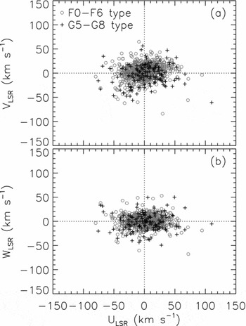
dex. However, they were unable to convincingly assign those stars to a known Galactic population. In our study, old metal-rich stars have different velocity dispersions from the early-type stars, i.e. the F0–F6 spectral type. Although the ranges of the space velocity components for two sub-samples are almost the same (Figure 21), F0–F6 spectral-type stars are concentrated relatively to lower space velocities, resulting in smaller velocity dispersions, while old metal-rich G5–G8 spectral-type stars are scattered to larger space velocities and therefore have relatively larger space velocity dispersions. Numerical values are given in Table 4. A comparison of the space velocity dispersions of two sub-samples indicates that old metal-rich G5–G8 spectral-type stars are members of the thick disc. Wilson et al. (Reference Wilson2011) favour the procedure ‘gas-rich merger’ for the formation of the thick disc. However, they state that a fraction of the thick disc stars could be formed by the ‘radial migration process’. The old metal-rich sub-sample in our study may be the candidates of the second procedure, i.e. they could have migrated radially from the inner disc of the Galactic bulge. Contrary to the F0–F6 spectral type stars, the G-type ones are old enough for such a radial migration.
$\text{[M/H]} \ge +0.4$
dex. However, they were unable to convincingly assign those stars to a known Galactic population. In our study, old metal-rich stars have different velocity dispersions from the early-type stars, i.e. the F0–F6 spectral type. Although the ranges of the space velocity components for two sub-samples are almost the same (Figure 21), F0–F6 spectral-type stars are concentrated relatively to lower space velocities, resulting in smaller velocity dispersions, while old metal-rich G5–G8 spectral-type stars are scattered to larger space velocities and therefore have relatively larger space velocity dispersions. Numerical values are given in Table 4. A comparison of the space velocity dispersions of two sub-samples indicates that old metal-rich G5–G8 spectral-type stars are members of the thick disc. Wilson et al. (Reference Wilson2011) favour the procedure ‘gas-rich merger’ for the formation of the thick disc. However, they state that a fraction of the thick disc stars could be formed by the ‘radial migration process’. The old metal-rich sub-sample in our study may be the candidates of the second procedure, i.e. they could have migrated radially from the inner disc of the Galactic bulge. Contrary to the F0–F6 spectral type stars, the G-type ones are old enough for such a radial migration.
Distribution of F0–F6 (○) and G5–G8 (+) spectral-type stars in the space velocity component planes in two panels: (a) (U, V) and (b) (U, W).
Space velocity dispersions for two sub-samples (units in km s−1).

The metallicity distributions with respect to age for different populations, i.e. TD/D ≤ 0.1, 0.1 < TD/D ≤ 1, 1 < TD/D ≤ 10, and 10 < TD/D, also show slopes. However, they are different than those for sub-samples defined by spectral types. They are smaller compared with the former. The application of two constraints, i.e. spectral type and population, to our sample results in metallicity distributions with respect to age similar to those obtained for spectral sub-samples alone, which indicates that spectral type is more effective in establishing an AMR relative to the population of a star, i.e. population type is not a strong indicator in the AMR.
Conclusion.
We obtained the AMR with the RAVE data, which have common features as well as differences with Hipparcos. Some differences in features can be explained with different constraints: (1) The AMR for the sub-samples F0–F3 and F3–F6 with stars younger than 6 Gyr in our study has almost the same trend of the AMR for Feltzing et al. (Reference Feltzing, Holmberg and Hurley2001)'s F-type stars younger than 4 Gyr with temperatures $3.83<\log T_{\text{eff}}{\rm \,(K)}\le 3.85$
and
$3.83<\log T_{\text{eff}}{\rm \,(K)}\le 3.85$
and $3.80<\log T_{\text{eff}}{\rm \,(K)}\le 3.83$
, respectively. They give the indication of a large slope. However, a few dozens of stars with age 4 < t < 9.5 Gyr and temperature
$3.80<\log T_{\text{eff}}{\rm \,(K)}\le 3.83$
, respectively. They give the indication of a large slope. However, a few dozens of stars with age 4 < t < 9.5 Gyr and temperature $3.80<\log T_{\text{eff}}{\rm \,(K)}\le 3.83$
in Feltzing et al. (Reference Feltzing, Holmberg and Hurley2001) which have a flat distribution do not appear in our study, confirming the accuracy of the ages estimated via the Bayesian procedure. The trend of the AMR becomes gradually flat when one goes to later spectral types in our study or to cooler stars in Feltzing et al. (Reference Feltzing, Holmberg and Hurley2001). The AMR for the thin-disc red clump giants in Soubiran et al. (Reference Soubiran, Bienaymé, Mishenina and Kovtyukh2008) confirms the large slope for the young stars and the flat distribution for the older ones, t>5 Gyr. (2) Substantial scatter in metallicity in our study was observed in all related studies (cf. Feltzing et al. Reference Feltzing, Holmberg and Hurley2001; Nordström et al. Reference Nordström2004; Soubiran et al. Reference Soubiran, Bienaymé, Mishenina and Kovtyukh2008). (3) In our study, we revealed that the metal-rich old stars are of G spectral type. These stars could have migrated radially from the inner disc or the Galactic bulge.
$3.80<\log T_{\text{eff}}{\rm \,(K)}\le 3.83$
in Feltzing et al. (Reference Feltzing, Holmberg and Hurley2001) which have a flat distribution do not appear in our study, confirming the accuracy of the ages estimated via the Bayesian procedure. The trend of the AMR becomes gradually flat when one goes to later spectral types in our study or to cooler stars in Feltzing et al. (Reference Feltzing, Holmberg and Hurley2001). The AMR for the thin-disc red clump giants in Soubiran et al. (Reference Soubiran, Bienaymé, Mishenina and Kovtyukh2008) confirms the large slope for the young stars and the flat distribution for the older ones, t>5 Gyr. (2) Substantial scatter in metallicity in our study was observed in all related studies (cf. Feltzing et al. Reference Feltzing, Holmberg and Hurley2001; Nordström et al. Reference Nordström2004; Soubiran et al. Reference Soubiran, Bienaymé, Mishenina and Kovtyukh2008). (3) In our study, we revealed that the metal-rich old stars are of G spectral type. These stars could have migrated radially from the inner disc or the Galactic bulge.
ACKNOWLEDGEMENTS
This work has been supported in part by the Scientific and Technological Research Council (TÜBİTAK) 210T162 and the Scientific Research Projects Coordination Unit of Istanbul University (Project number 14474).
We thank Dr. Bjarne Rosenkilde Jørgensen, Mr. Tolga Dinçer, and Mr. Alberto Lombardo for helping us to improve the code related age estimation. Funding for RAVE has been provided by the Australian Astronomical Observatory, the Leibniz-Institut fuer Astrophysik Potsdam (AIP), the Australian National University, the Australian Research Council, the French National Research Agency, the German Research Foundation, the European Research Council (ERC-StG 240271 Galactica), the Istituto Nazionale di Astrofisica at Padova, The Johns Hopkins University, the National Science Foundation of the USA (AST-0908326), the W. M. Keck Foundation, the Macquarie University, the Netherlands Research School for Astronomy, the Natural Sciences and Engineering Research Council of Canada, the Slovenian Research Agency, the Swiss National Science Foundation, the Science and Technology Facilities Council of the UK, Opticon, Strasbourg Observatory, and the Universities of Groningen, Heidelberg and Sydney. The RAVE website is http://www.rave-survey.org.
This publication makes use of data products from the Two Micron All Sky Survey, which is a joint project of the University of Massachusetts and the Infrared Processing and Analysis Center/California Institute of Technology, funded by the National Aeronautics and Space Administration and the National Science Foundation. This research has made use of the SIMBAD, NASA's Astrophysics Data System Bibliographic Services and the NASA/IPAC ExtraGalactic Database (NED), which is operated by the Jet Propulsion Laboratory, California Institute of Technology, under contract with the National Aeronautics and Space Administration.


