


Introduction
For investigating interactions between glaciers, monitoring climate and environmental change must involve the atmosphere and ocean, both in the Arctic and globally. It is important, therefore, to comprehensively analyse processes occurring at the interface between the cryosphere, hydrosphere and atmosphere, i.e. within an ice cliff and in its immediate vicinity. Arctic tidewater glaciers are also responding to global warming with increasing frontal ablation intensity (Kochtitzky and others, Reference Kochtitzky2022). More intensive calving dynamics and ice cliff melting alter a glacier's overall mass balance and geometry. Long-term environmental monitoring in glaciated regions indicates that this trend is going to intensify in the coming decades (IPCC, 2019). Several calving models have been developed based on long-term observations and comparative analyses of large groups of glaciers. They are founded on relationships between calving rate and factors like water depth (Pelto and Warren, Reference Pelto and Warren1991), glacier velocity (Jania, Reference Jania1988a; Van der Veen, Reference Van der Veen1996), fracturing due to longitudinal stretching associated with large-scale velocity gradients along a glacier (Benn and others, Reference Benn, Warren and Mottram2007) and rising water levels in crevasses, which increase their depth (De Andrés and others, Reference De Andrés, Otero, Navarro and Walczowski2021). The calving rate of a glacier changes seasonally. Short-term changes in glacier velocities are only weakly correlated with calving intensity. It is also difficult to link short-term changes in calving intensity with basin depth (Sikonia, Reference Sikonia1982; Van der Veen, Reference Van der Veen1999) or the density and pattern of crevasses (Benn and others, Reference Benn, Warren and Mottram2007). These factors do not change so rapidly.
As the position of the glacier terminus slowly changes, melting and ice cliff undercutting at the waterline may have a significant impact on calving intensity, a process that is dominant at Hansbreen (Vieli, Reference Vieli2001). Several studies of iceberg melt rates have noted that melting within the undercut notch at the waterline proceeds faster than convection-driven melting across the entire subaqueous ice surface (El-Tahan and others, Reference El-Tahan, Venkatesh and El-Tahan1987). The development of undercut notches within tidewater glacier fronts has also been observed (Röhl, Reference Röhl2006; Petlicki and others, Reference Petlicki, Cieply, Jania, Prominska and Kinnard2015). Numerous studies recently undertaken in Alaska, Greenland and Svalbard stress the importance of subglacial discharge as a driver of melting at the waterline across the glacier front (e.g. Motyka and others, Reference Motyka, Hunter, Echelmeyer and Connor2003, Reference Motyka2011, Reference Motyka, Dryer, Amundson, Truffer and Fahnestock2013; Bartholomaus and others, Reference Bartholomaus, Larsen and O'Neel2013; Xu and others, Reference Xu, Rignot, Fenty, Menemenlis and Flexas2013; Kimura and others, Reference Kimura, Holland, Jenkins and Piggott2014; Caroll and others, Reference Caroll2015; Cowton and others, Reference Cowton, Slater, Sole, Goldberg and Nienow2015; Fried and others, Reference Fried2015; Rignot and others, Reference Rignot, Fenty, Xu, Cai and Kemp2015; Slater and others, Reference Slater, Goldberg, Nienow and Cowton2016; Bendtsen, Reference Bendtsen2017). De Andrés and others (Reference De Andrés, Otero, Navarro and Walczowski2021) highlight the dependence of submarine melting in response to transient fjord temperature and subglacial discharges which, together with crevasse water depth, influence the calving rate of Hansbreen. A study on Kronebreen and Tunabreen in Svalbard indicates that calving is strongly correlated with sea temperature (Luckman and others, Reference Luckman2015).
The aim of this study was to determine the seasonal and inter-day variability of factors mediating calving intensity as the dominant component of Hansbreen frontal ablation. The mechanism of frontal ablation was studied with reference to detailed observations of marine, atmospheric and glaciological factors influencing glacier calving.
We have introduced a few indices in order to better characterize frontal ablation on Hansbreen:
• the calving extent ratio (CER), defined as the percentage of the ice cliff length affected by calving in relation to the ice cliff's entire length. It provides information on calving activity on specific days of the period analysed.
• the calving interval index (Cii), defined as the number of days without calving episodes at a given location on the ice cliff in 10 d periods. It is calculated as the mean for the calving front, and separately for each designated sector on the ice cliff, and provides information on the mean duration of intervals between calving episodes.
• the tortuosity index, defined as the ratio between the ice cliff length and the length of the straight line connecting its endpoints. It provides information on the types of submarine melting mechanisms prevailing in a given period. Wave-driven submarine melting affects the ice cliff frontally, which straightens the glacier terminus line. Submarine melting driven by subglacial water discharge leads to varying melt rates on the ice cliff, which increases its tortuosity.
Study area
The field studies took place within the frontal zone and forebay of Hansbreen, which flows into Hansbukta, a bay in Hornsund fjord (henceforth: Hornsund) in southern Spitsbergen (Fig. 1). Despite their considerable diversity, the glaciers near the fjord are representative of the entire island of Spitsbergen in terms of geometry and annual mass balance (Jania, Reference Jania1988b; Grabiec and others, Reference Grabiec, Jania, Puczko, Kolondra and Budzik2012). We chose Hansbreen as the study area because of its long and detailed observational records and well-developed monitoring infrastructure.
Location map of Hansbreen and research infrastructure used in the project. The labels (‘0–2 m’, ‘20 m’) indicate the depths of the water pressure and temperature sensors. WSC, West Spitsbergen Current (warm); ESC, East Spitsbergen Current (cold) (basemap: Kolondra, Reference Kolondra2018).

Hansbreen is a grounded polythermal glacier c. 15 km long and 2.5 km wide on average, and c. 51 km2 in area. Its active ice cliff is 1.7 km in length with a mean front freeboard height of 30 m (Błaszczyk and others, Reference Błaszczyk2021). At the glacier margins, the ice front is not as tall above the water as at the active centre, where it is c. 15 m high and inclined at a smaller angle. Since the end of the 19th century, the glacier front has retreated 2.7 km (Oerlemans and others, Reference Oerlemans, Jania and Kolondra2011). The mean annual velocity within the glacier's frontal zone is c. 140 m a−1 (Błaszczyk and others, Reference Błaszczyk2021)
The glacier terminates in Hansbukta, one of the many branches of Hornsund. It has a maximum depth of over 80 m. The forebay of Hansbreen is not deep enough for the glacier terminus to float. The bay's relief is varied, consisting of transverse ridges with annual and terminal, regular small steps, flat-bottomed depressions and irregular slopes. The longest underwater ridge, consisting of terminal moraine situated c. 2.5 km from the glacier front at a depth of 15–17 m, is c. 3 km long and is located where the bay opens into Hornsund (Ćwiąkała and others, Reference Ćwiąkała2018).
Hornsund, in turn, opens westwards into the Greenland Sea. Its mouth is c. 14.5 km wide, which is sufficient to allow the free penetration of ocean water into it (Herman and others, Reference Herman, Wojtysiak and Moskalik2019). Hornsund has a mean depth of c. 90 m and a maximum depth of >260 m (Moskalik and others, Reference Moskalik, Grabowiecki, Tęgowski and Żulichowska2013, Reference Moskalik, Błaszczyk and Jania2014). Hornsund's coastline is heavily indented and features numerous peninsulas and bays, including Isbjørnhamna, Burgerbukta and Brepollen Bays (Swerpel, Reference Swerpel1985). The hydrology of Hornsund is complex and highly variable as a result of the considerable masses of fresh water discharged into it by glaciers and snow, melting, icebergs, rivers, runoff and precipitation (Błaszczyk and others, Reference Błaszczyk2019), and also the sea-ice conditions (Jakacki and others, Reference Jakacki, Przyborska, Kosecki, Sundfjord and Albretsen2017; Promińska and others, Reference Promińska, Cisek and Walczowski2017, Reference Promińska, Falck and Walczowski2018).
The West Spitsbergen Current (Fig. 1), flowing off the west coast of Spitsbergen, transports warm, highly saline Atlantic waters northwards to the Arctic Ocean (Zblewski, Reference Zblewski2007). Its main stream moves water masses along the continental slope, although numerous eddies have been recorded within it (Piechura and others, Reference Piechura, Beszczyńska-Moller and Psiński2001), which complicates the water circulation off Spitsbergen. Heat transport within the current is pulsating by nature (Walczowski and Piechura, Reference Walczowski and Piechura2006), and the range and spatial distribution of individual water streams are highly variable (Walczowski and others, Reference Walczowski, Piechura, Osinski and Wieczorek2005). Between 1999 and 2020, the volume of Atlantic Water on the southern Spitsbergen shelf increased by 8%, an increase that has been particularly conspicuous in the last decade (Strzelewicz and others, Reference Strzelewicz, Przyborska and Walczowski2022).
As a consequence of this ocean circulation, two types of seawater can enter Hornsund. One type is warm, saline water transported by the West Spitsbergen Current, with temperature of 3.5–6.5°C, while the other is cold water from the Sørkapp Current (a continuation of the East Spitsbergen Current) with seasonally variable salinity. In winter, the temperature of these waters falls below −1.5°C while in summer it does not exceed 1.5°C (Wiśniewska-Wojtasik, Reference Wiśniewska-Wojtasik2005).
Oceanographic studies conducted in 2015 and 2016 found that the temperature and salinity in Hansbukta were seasonally variable. The mean temperature was lowest in winter (−1.8°C), increased rapidly in late spring and early summer, and peaked in midsummer (2°C), before gradually dropping through autumn and into winter. The mean salinity, on the other hand, peaked in early spring (35 PSU), dropped to its lowest value by midsummer (32 PSU), and gradually rose through autumn and winter (Glowacki and others, Reference Głowacki, Moskalik and Deane2016; Moskalik and others, Reference Moskalik2018).
Data and methods
Atmospheric, oceanographic and glaciological data
Meteorological, oceanographic and glaciological data were used in regression analysis to identify the environmental factors driving calving. Meteorological data, primarily air temperature (mean, minimum and maximum) and precipitation, were sourced from the meteorological bulletins of the Stanisław Siedlecki Polish Polar Station in Hornsund.
Sea temperature was recorded at the surface of the glacier forebay and at its bottom at 20 m depth (Fig. 1). Surface water temperature was recorded with a HOBO U20-001-04 sensor at 5 min intervals from 12 July to 31 December 2015, and from 29 May to 12 September 2016. Sea temperature at 20 m depth was recorded at 15 min intervals from 1 June 2014 to 16 May 2016 using a Hobo Water Temp Pro v2 U22-001 installed at the bottom of Hansbukta (Fig. 1).
From 10 June 2015 to 2 February 2016, and from 30 June 2016 to 22 May 2017, an RBR Virtuoso pressure sensor, which records pressure in burst mode, was deployed at the bottom of Hansbukta (depth 20 m). From this record of water pressure variations, we calculated tidal amplitudes and daily mean wave heights. For the period without measurements, tidal amplitudes were determined using the AODTM-5 Arctic Ocean Tidal Forward Model (Padman and Erofeeva, Reference Padman and Erofeeva2004).
Four velocity stakes (A–D) were installed along the glacier front to measure its velocity (Fig. 1). The positions of all the stakes were measured with a Leica 1200 differential GPS, on average every 3–4 d from 14 July to 13 August 2015. Velocity was also analysed on the basis of stake No. 4, located approximately 3.5 km upstream of the Hansbreen glacier terminus (S4 in Fig. 1).
Calving intensity
From 1 January 2011 to 13 September 2016, the transformations taking place at the Hansbreen front as a result of calving were monitored using a time-lapse camera (Canon EOS 1000D, 18 mm focal length lens, Harbotronic DigiSnap 2700 remote shutter release system). Such cameras have already been used in many studies of calving intensity (e.g. Petlicki and others, Reference Petlicki, Cieply, Jania, Prominska and Kinnard2015; Medrzycka and others, Reference Medrzycka, Benn, Box, Copland and Balog2016; Mallalieu and others, Reference Mallalieu, Carrivick, Quincey, Smith and James2017; Otero and others, Reference Otero2017; Minowa and others, Reference Minowa, Podolskiy, Sugiyama, Sakakibara and Skvarca2018; Köhler and others, Reference Köhler2019). Our camera was installed on the Baranowski Peninsula (Fig. 1) and took images of the Hansbreen ice cliff at 1 h intervals. In August 2011, the camera was c. 0.95 km distant from the ice cliff centre, while in August 2016 this distance was c. 1.4 km. One image was selected (usually taken at midnight) for each day of the period analysed. Individual calving events were identified and their areas marked manually based on comparative analyses of images from two consecutive days using ArcGIS 10.5 software (Fig. 2). We interpreted local changes in the ice cliff's colour or shape as evidence that calving had occurred during the time interval separating both images. Subsequently, the ice cliff length where calving had occurred was measured at the waterline for each day of the analysis period and compared to the total length of the cliff visible in the images. Thus, we define the ‘calving extent ratio’ (CER) as the percentage of the ice cliff length affected by calving in relation to its entire extent for every day of the period analysed.
Zoomed portion of the Hansbreen ice cliff with examples of calving episodes marked on it. The upper image was taken on 2 September 2015 at 00.00 h, the lower one on 3 September 2015 at 00.00 h. The red polygons indicate sites where changes caused by calving were recorded.

Changes in the ice cliff were also observed during the polar night by moonlight or an intense Aurora Borealis. Unfortunately, it was only rarely possible to compare images taken on two consecutive days. Images suitable for analysis were less frequent. As Hansbreen seldom calves in winter, daily analysis of calving was not normally required. If weather conditions and poor light precluded analysis for several days during which calving was recorded, that period was not analysed further, since it was impossible to date the calving event exactly. On the other hand, if no changes to the glacier front had taken place during that period, a CER of zero was assigned to each date within it. Recurrent data gaps also occurred as a result of random events such as camera power failure. If there were occasional slight changes in camera angle, the observation days affected were omitted from the analysis, which continued with comparisons of subsequent images, taken after the camera's position had already changed.
Error analysis of the CER method required the varying position of the glacier terminus with respect to the camera's position to be taken into account, because the real pixel size in the field depends on the distance from the camera to the given location on the ice cliff. This parameter is time-variable owing to glacier recession; it also varies spatially along the terminus. The distance was found by identifying the same positions of the terminus on georeferenced Landsat 8 satellite images and time-lapse images taken on the same day. Because of cloud cover, applicable Landsat scenes were randomly distributed throughout the study period (2014–2016). For the final calculation of terrain pixel sizes, terminus-camera distances, a camera focal length of 18 mm and the physical size of pixels on the camera matrix of 5.7 μm×5.7 μm were used. This error analysis – performed for limited (cloud-free) Landsat 8 scenes – revealed that a mean error of 2.2% was obtained for a fixed camera–glacier terminus distance.
Relationships between calving intensity and physical parameters of the glacier's immediate surroundings (air temperature, sea temperature, precipitation, tides, wave height and period, glacier velocity) were studied. Based on CER data obtained from the time-lapse camera, along with parameters registered or measured simultaneously, we analysed the statistical relationships between individual factors and CER using linear regression.

The ‘calving interval index’ (hereafter Cii) at a given location within the ice cliff was introduced to quantify calving activity. Each registered calving event was assigned to one or more of the 21 sectors dividing the glacier front (Fig. 3). Sectors in which calving events occurred were assigned a value of 1, while those where no calving was recorded were not marked. Subsequently, the entire analysis period was divided into 10 d periods for which continuous data sequences were available. The mean number of days without calving events in each sector was calculated for each period, the results reflecting Cii at a specific location on the cliff. A result of Cii = 0 should be interpreted as the average time between consecutive calving events that were shorter than a day. In contrast, a result of Cii = 10 means that the interval between calving events at the same location was equal to or longer than 10 d. The lower the Cii value, the more frequently calving occurred in the sector in question. Cii is thus the reverse of the calving intensity. Hence, mean values of the parameters describing the element in question for each environmental factor potentially relevant to calving were calculated for the same 10 d periods or, in the case of precipitation, the sum was calculated. The last step was a linear regression analysis, which was used to compare mean values of individual environmental parameters with mean Cii calculated as described above for a specific location. Statistical analyses were done for specific factors, and differences in their importance at various times during the year were examined.
Method of estimating Cii (calving interval index) at a specific location within the cliff. The number 1 in the matrix indicates sectors in which calving episodes occurred on a given day of analysis. The blue polygon on the ice cliff represents an area of calving episode, which was registered on 23 May 2016. The blue numbers indicate the five sectors with the lowest counts of days with calving events, and the red numbers the five sectors with the highest counts of days with such events (the figure is based on a photograph taken on 23 May 2016).

For the same 10 d windows, Cii was also calculated for each sector separately. Linear regression analysis was also performed to compare the results with environmental parameters (mean sea temperature, mean air temperature, glacier velocity, wave period and height). The significance level for all statistical analyses was fixed at α = 0.05.
Analysis of changes in ice cliff tortuosity
Different calving intensities in particular sectors of the Hansbreen ice cliff are shown above by the frequency of iceberg break-off events leading to diversified glacier front retreat. Thus, the shape of the ice cliff line's horizontal projection at sea level would be more or less complicated and would therefore represent the cliff's effective length. This could be used to parametrize the tidewater glacier's frontline shape by the tortuosity index during different periods of the year. This index is the ratio of a coastline's length to the length of a straight line connecting its endpoints. The tortuosity index has been used to analyse ice cliffs in order to identify tidewater glacier surges on Svalbard (Szafraniec, Reference Szafraniec2020). Changes in ice cliff tortuosity can indicate changes in the drivers of frontal ablation. Melting controlled by estuarine circulation increases the ice cliff's tortuosity because melting is faster near subglacial meltwater discharges. In addition, the greater the convolution of the ice cliff, the larger the contact surface with the sea and thus the melting efficiency. Wave-controlled melting is almost uniform along the terminus and leads to ice cliff alignment.
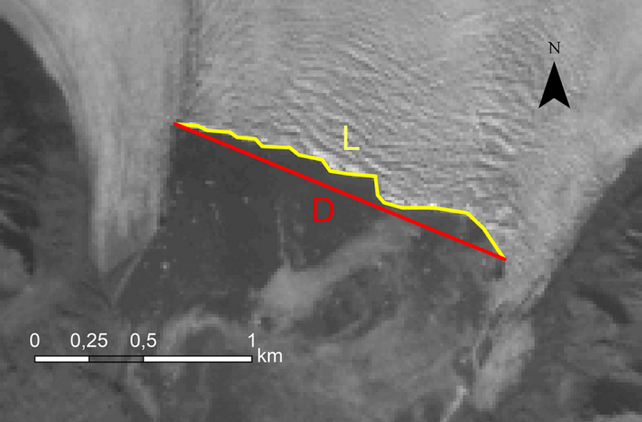
The actual length of the coastline was compared to that of the corresponding straight line by calculating the front tortuosity index (If) according to the following formula:

where L is the length of the measured along the ice cliff [m] and D is that of the segment joining the same ice cliff endpoints (Spagnolo and others, Reference Spagnolo, Llopis, Pappalardo and Federici2008). The Hansbreen cliff tortuosity index for 2013–2018 was calculated for 38 scenes based on Landsat 8 satellite geocoded images with a spatial resolution of 15 m (band 8 – panchromatic) obtained from the USGS database (https://earthexplorer.usgs.gov). The selection criterion for images was that visibility (dependent on weather conditions) had to be sufficiently good to enable the glacier front to be precisely traced. The numbers of images available for individual years in the USGS database varied widely. The active glacier front was mapped for each image and a straight line drawn to connect the endpoints of this ice cliff trace (Fig. 4).
Method of calculating the calving front tortuosity index. L, length of coastline [m]; D, length of segment joining the ice cliff endpoints (background: USGS Landsat 8, 2015-09-08).
When tracing the front line, we eliminated lateral fragments of the glacier terminus where calving events had not been observed or were rarely noted during the entire ablation season. We focused on the active part of the terminus, ignoring the stagnant ice on either side. An important aspect of this method was that images of the same resolution were used and fixed distances between consecutive vertices of the polyline drawn on the glacier front were maintained. Those issues were important in order to eliminate the so-called coastline paradox, i.e. where a single section of coastline was analysed, its length L would increase in proportion to the scale of the image on the basis of which it was plotted.
Application of the tortuosity index highlights changes in the development level of an ice cliff over time using a parameterized method: mechanisms leading to ice cliff lengthening or shortening can be investigated in this way.
Results
Calving extent ratio vs environmental factors
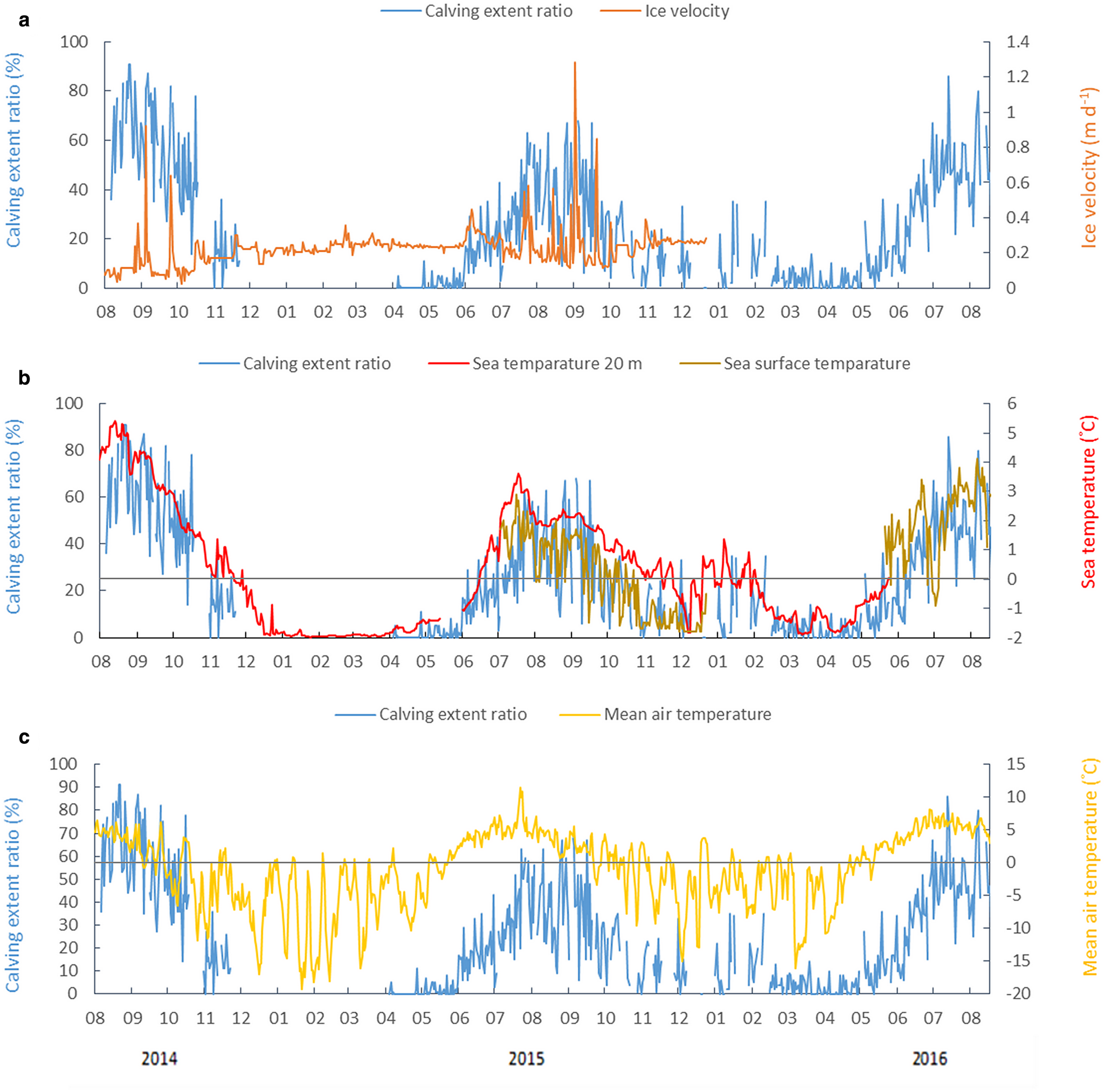
The CER of Hansbreen varied seasonally. CER increased markedly in late May and early June, and peaking in summer. Thereafter, CER declined slowly, dropping to a minimum in winter and spring (Fig. 5). This rhythm corresponds to the cycle of changes in both sea (Fig. 5b) and air (Fig. 5c) temperature. However, linear regression demonstrated that the relationship of CER with sea temperature, especially at 20 m depth (R 2 = 0.71) (Fig. 6; Table 1), was much stronger than that with mean air temperature (R 2 = 0.3; Table 1). There was also positive but weaker correlation with mean daily surface water temperature (R 2 = 0.4; Table 1). Although specific intense rainfall events were associated with increased calving, no relevant relationship was found over longer periods, nor was any relationship demonstrated between CER and factors like glacier ice velocity, tidal amplitude or mean wave height.
Distribution of the daily calving extent ratio vs (a) ice velocity measured on the basis of stake No. 4, located approximately 3.5 km upstream of the Hansbreen glacier terminus (S4 in Fig. 1), (b) sea temperature recorded at the surface and at depths of 20 m (sea sensors in Fig. 1) and (c) mean air temperature measured at the Polish Polar Station (weather station in Fig. 1).
(a) Scatter plot of the Hansbreen calving extent ratio [in % of the ice cliff face] vs mean sea temperature [20 m] cf. Figure 5b. (b) Linear regression residuals.

Relationship between calving extent ratio and selected environmental factors

R and R 2 values were bolded when the p-value was less than the statistical significance level fixed at α = 0.05.
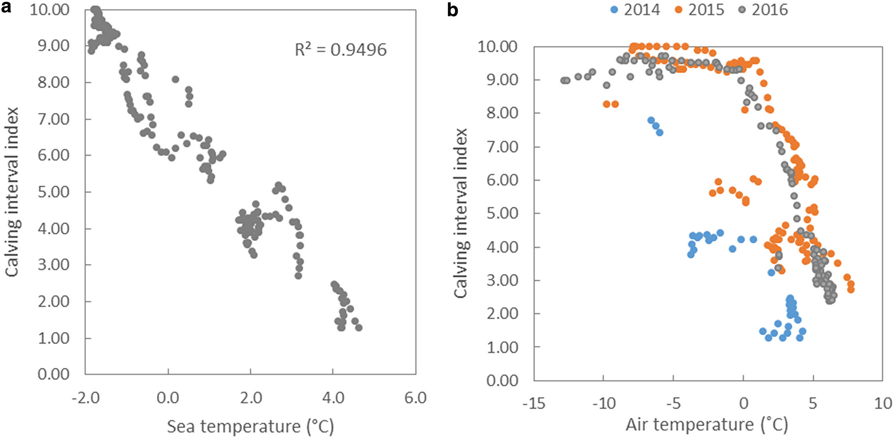
There was a very strong negative correlation between average Cii and sea temperature recorded at 20 m depth (R 2 = 0.95) (Fig. 7a; Table 2). There were also weaker negative correlations with mean air temperature (R 2 = 0.54) (Fig. 7b; Table 2), mean surface water temperature (R 2 = 0.37) (Table 2) and total rainfall (R 2 = 0.26) (Table 2). On the other hand, no significant relationship with glacier velocity was found (Fig. 5a; Table 2).
Scatter plots of mean calving interval index and (a) mean sea temperature [20 m]; (b) mean air temperature.
Relationship between calving interval index and selected environmental factors

R and R 2 values were bolded when the p-value was less than the statistical significance level fixed at α = 0.05
Although statistical analysis did not reveal any correlation with the mean wave height or mean wave period over the entire study period (Table 2), the significance of the mean wave period did change during the year. No correlation was found for July–mid-September (Fig. 8a.; Table 2), but for mid-September–April 9, R 2 was equal to 0.91 (Fig. 8b; Table 2).
Scatter plots of mean calving interval index and mean wave period [s] from July to 14 September (a) and from 15 September to April 9 (b).

In those locations on the Hansbreen front with the highest number of days with calving events (sectors marked with red numbers on Fig. 3), statistical analysis still indicated that sea temperature mediated the average time elapsing between successive calving events (R 2 = 0.82). In those sectors, air temperature also turned out to be of greater significance than shown by the analysis for the entire front area (R 2 = 0.64). R 2 of the Cii–mean wave period relationship for the entire period analysed was 0.18 (for July–mid-September it was 0, and for mid-September–9 April it was 0.7).
The strongest mean Cii–sea temperature relationship (R 2 = 0.88) was also found in sectors with the fewest days with calving events (sectors marked with blue numbers in Fig. 3), i.e. the sectors in the lateral parts of the glacier termini. In those locations, air temperature decreased markedly (R 2 = 0.39) but rainfall increased (R 2 = 0.32) in importance. The mean wave period in those sectors was not significantly correlated with mean Cii within a sector (R 2 = 0.18). As in the analyses conducted for all sectors and for the five sectors with the most days with calving events, R 2 was the lowest for period July–mid-September (0) and the highest for mid-September–9 April (0.54).
No significant relationships were found in either group of sectors between Cii, wave height and glacier velocity.
Regression analysis performed for a single sector also shows the strongest relationship between Cii and sea temperature recorded at 20 m depth. R 2 calculated for each sector separately was 0.62–0.85 (Fig. 9). By basing the analysis on sea surface temperature, we obtained significantly lower and more diverse values of R 2 (0.03–0.63). The analysis for 15 September–9 April indicates a strong relationship between Cii and the wave period (0.34–0.87). Analysis of Cii and average air temperature above 0˚C for September–October yielded a broad range of R 2 (0.01–0.65). We associate this with the degree of development of the glacial drainage system, which reaches its maximum efficiency at the end of or just after the ablation season, and this elicits a rapid response to rising air temperature in the form of increased subglacial runoff. A stronger statistical relationship between Cii and average air temperature was noted in sectors where ‘glacier gates’ reflecting outflows of subglacial water were frequently observed (Fig. 10). Hansbreen's subglacial system is stable and is not subject to fundamental reorganization (Decaux and others, Reference Decaux, Grabiec, Ignatiuk and Jania2019).
Relationship between calving interval index and selected environmental factors for each sector separately. Blue numbers indicate the five sectors with the fewest calving days, and red numbers show the five sectors with the most calving days. The colour scale indicates the intensity of the relationship: the higher the coefficient of determination, the more intense the red colour, and the lower the value of R 2, the more intense the blue colour.

Location of a typical embayment in the Hansbreen terminus associated with the ‘glacier gate’, with a forebay plume. Grey dot – position of time-lapse camera. Part of Hansbreen ice cliff with a stronger relationship between Cii and average air temperature is marked with the red ellipse (background: USGS Landsat 8, 2015-09-15).

Changes in coastline tortuosity
The mean tortuosity index of Hansbreen's front, calculated from 38 satellite images for April 2013–March 2018, was 1.07. Hansbreen's cliff line is relatively even. Because very different numbers of satellite images were available for particular years, and intervals between images for which the index could be calculated varied in duration, how exactly its value was distributed in the annual cycle could not be determined. However, these relationships, recurring every year, were observed: the index always peaked in summer (from July to September), its values being significantly higher than in the preceding and succeeding springs (Fig. 11). Calculating the tortuosity index is less time-consuming than CER and Cii. The tortuosity index is easily applicable for analysing annual changes in frontal ablation.
Changes in the tortuosity index of the Hansbreen glacier cliff in 2013–17 vs mean daily air and sea temperature.

Discussion
This analysis indicates that sea temperature is governed principally by frontal ablation on Hansbreen. Submarine melting in frontal ablation was recognized as a crucial factor in Alaska (Motyka and others, Reference Motyka, Hunter, Echelmeyer and Connor2003; Bartholomaus and others, Reference Bartholomaus, Larsen and O'Neel2013; Sutherland and others, Reference Sutherland2019; Jackson and others, Reference Jackson2022), Greenland (Xu and others, Reference Xu, Rignot, Fenty, Menemenlis and Flexas2013) and also Svalbard, where a strong relationship was found between sea temperature measured at depths of 20–60 m and the frontal ablation rate of Kronebreen (R 2 = 0.84) and Tunabreen (R 2 = 0.8) (Luckman and others, Reference Luckman2015). Our study points to a very clear inverse relationship between Cii at a particular location and sea temperature at 20 m depth (Fig. 7a), which is associated, in turn, with the dependence of submarine melting on sea temperature (De Andrés and others, Reference De Andrés, Otero, Navarro and Walczowski2021) and undercut formation (Slater and others, Reference Slater, Benn, Cowton, Bassis and Todd2021).
Glaciological factors also influence frontal ablation (Benn and others, Reference Benn, Warren and Mottram2007), but in our opinion, by controlling local undercutting depth, they generate calving episodes (Fig. 12). When the melt undercut reaches a critical depth, ice is lost from the glacier front through calving. Subsequently, there follows a period of stagnation that has to elapse before the next critical undercut depth can be reached. We argue, furthermore, that the melt undercuts generating successive calving events at the same location occur at similar depths. Otherwise, variations in the critical undercut depth activating calving would affect the melting time, and Cii and sea temperature would not be as strongly correlated (Fig. 7a; Table 2).
Diagram of the relationships between the factors governing frontal ablation: during summer, when melting below the waterline mediated by estuarine circulation is dominant (green rectangles); when subglacial outflow is less intensive, i.e. when melting at the waterline governed by wave action dominates (grey rectangles). The glaciological factors influencing calving are also listed (blue rectangles).

We have distinguished two calving mechanisms in Hansbreen, depending on how and where melt undercuts appear (Fig. 12). Melt undercutting in the deeper parts of the cliff takes place when frontal ablation is at its most intense. The upward movement of water, ensuring its continuous exchange and hence heat exchange at the melting ice front, is generated mostly by subglacial meltwater discharge (e.g. Motyka and others, Reference Motyka, Hunter, Echelmeyer and Connor2003; Motyka and others, Reference Motyka, Dryer, Amundson, Truffer and Fahnestock2013; Xu and others, Reference Xu, Rignot, Fenty, Menemenlis and Flexas2013; Fried and others, Reference Fried2015; Schild and others, Reference Schild2018, Vallot and others, Reference Vallot2018). The principal factors governing melting are:
• temperature of seawater involved in the estuarine circulation is related to inflows of warmer or colder sea water masses to the fjord from the open sea;
• the factors responsible for the intensity of the subglacial water discharge that generates the estuarine circulation.
We consider that the factors responsible for the intensity of subglacial discharge include air temperature as a proxy for the superficial ablation intensity of the glacier surface (Fig. 7b); rainfall events (Table 2); the degree to which the glacial channel system has been ramified and is filled by sediments; short-term discharges of water retained on the surface and within the glacier (e.g. in crevasses). The estuarine circulation itself is also affected by additional water movements within the bay, e.g. currents, tides and wave motion. The submarine melting mechanism driven by estuarine circulation increased the tortuosity of the ice cliff (Fig. 11). Sikonia (Reference Sikonia1982) observed the formation of a large embayment within the Columbia Glacier ice cliff after heavy rains and the glacial lake outburst.
The second important mechanism driving calving is the melting of the glacier cliff near the water surface (Fig. 12); as a result, an undercut notch is formed (Fig. 13). This process depends on surface water temperature and wave motion (e.g. White and others, Reference White, Sapulding and Gominho1980; Vieli, Reference Vieli2001; Petlicki and others, Reference Petlicki, Cieply, Jania, Prominska and Kinnard2015). Based on the strong relationship between Cii and the wave period from 15 September to April and the weak one from July to 14 September, we consider this mechanism to be dominant outside the ablation period (Fig. 8b). Undercut melting at the waterline then proceeds faster than in the deeper submarine parts of the ice cliff. Its intensity is limited by sea ice or ice mélange on the surface of Hansbukta. A surface accumulation of ice pack or brash ice of glacial origin dampens wave motion and lowers surface water temperature, significantly reducing the waterline melting rate.
Part of Hansbreen's ice cliff with an undercut notch (red ellipse) above the waterline at low tide.

There is a perceptible annual cycle of changes in calving intensity and in the importance of factors triggering this process (Fig. 14). Based on our observations of calving activity and environmental parameters, we interpret the annual calving cycle as follows: in winter, seasonal sea ice is frequently present, so melting at the waterline is not possible (period A in Fig. 14). The importance of winter subglacial discharge, if any, is minimal. Therefore, submarine melting either does not occur or it plays a negligible role in ice cliff undercutting. But once the sea ice has disappeared, melting at the waterline begins (period B in Fig. 14). Sea temperature is still low, but there is wave motion and energy is released. Thus, the slow ice cliff melting rate and development of undercuts generate some calving events. Surface melting usually starts in June, and from then on, discharge and estuarine circulation gradually become more important for the melting mechanism in the deeper parts of the ice cliff (period C in Fig. 14). In 2015, melting began on 6 June (Decaux and others, Reference Decaux, Grabiec, Ignatiuk and Jania2019). At this time, with rising mean daily temperature, rainfall becomes more frequent, snow cover melts and disappears, the subglacial channel system becomes more efficient, and estuarine circulation-driven submarine thermoabrasion becomes more significant for calving than notch undercutting in the cliff at the water surface.
Annual calving cycle – changes in significance of specific marine factors during the year. A – period with sea-ice cover; B – period with melting at the waterline; C – period with melting contributed to by the estuarine circulation; ‘Mean’ is the mean CER calculated for individual months from the data for multi-annual period 2011–16, shown with thin coloured lines as depicted in the legend.

Rainfall is heaviest later in summer when the snow cover is reduced to a minimum and air temperature is relatively high. During this period, the glacial channel system is now fully efficient and cliff undercutting is mostly driven by melting contributed to by the estuarine circulation. As sea temperature is markedly higher, frontal ablation is now extremely intense. This stage lasts until the melt season ends: in 2015 this was on 10 October (Decaux and others, Reference Decaux, Grabiec, Ignatiuk and Jania2019).
The next stage of the annual cycle, which occurs in autumn, is when the importance of melting due to glacial discharge wanes (second period B in Fig. 14). This is related to the following factors:
• lower air temperature and thus cessation of superficial ablation;
• more snowfall events than rainfall events;
• the appearance of continuous snow cover;
• the gradual closure of subglacial channels.
This period is dominated by melting at the waterline, but as sea temperature is continually falling, calving is much less intense than in summer. Nevertheless, because water has a high thermal capacity, its temperature falls slowly. Although sea water motion is stimulated by only weak factors, calving events sometimes occur even in late December or early January. Melting at the waterline continues until sea ice appears. Frontal ablation ceases for as long as an ice cover is present. The glacier terminus thus advances seasonally (cf. Błaszczyk and others, Reference Błaszczyk2021). Vieli (Reference Vieli2001) also noted the greater importance of melting at the waterline on frontal ablation on Hansbreen as the terminus position slowly changes.
This cycle will not proceed according to the above scheme in exactly the same manner each year as it will be modified by the different thermal properties of the seawater masses flowing into Hornsund. In winter, for example, relatively warm water has sometimes been observed to enter the fjord as an intake from the West Spitsbergen Current, and some calving has taken place as a result. In summer, by contrast, cold Sørkapp Current waters could episodically enter Hornsund, significantly retarding calving. Deviations from the above scheme have also occurred with atypical sea-ice patterns. There have been winters when the sea-ice cover, which prevents cliff undercutting, persisted for a much shorter time than usual, so some limited calving did occur.
Sea temperature is of paramount importance when determining the time elapsing between successive calving events at a particular location along the glacier terminus. Even intensive circulation of cold water near the cliff at a temperature that is close to the melting point will not significantly accelerate ice-wall undercutting. In light of this observation, the factors driving glacial discharge, i.e. air temperature, which is responsible for surface ablation, rainfall (less important than air temperature), the ramification of the glacial channel system, the degree to which the channels are unobstructed and snow cover (which retains rainwater), should be treated as secondary factors in comparison to seawater temperature. Being episodic in nature, violent discharges of water trapped on the surface or within the glacier will be of minor importance. A tertiary factor is wave motion, which drives melting at the waterline. Also important is the presence of sea ice, which limits or prevents melting on the water surface. Subsidiary factors include other seawater movements, i.e. other currents and tides, in the bay, which modify the estuarine circulation and indirectly affect ice cliff melting.
We are aware that different calving styles occur at Hansbreen's terminus, including buoyancy-driven calving from the submarine part of the ice cliff. For example, submarine calving events were detected and analysed with passive underwater acoustics (Glowacki and others, Reference Glowacki2015). However, we were unable to detect such events because the temporal resolution of the time-lapse images was relatively low. Most importantly, surface water currents in Hansbukta cause significant drift (Moskalik and others, Reference Moskalik2018). This is why the primary origin of icebergs and growlers cannot be unequivocally identified. Nevertheless, we assume that submarine calving events do not play a major role in driving calving events above the waterline. Otherwise, the observed high correlation between water temperature, as a proxy of melting, and Cii could not be calculated. Moreover, studies conducted in similar settings show that submarine calving often produces the largest blocks of ice but usually accounts for only a few per cent of all calving events (e.g. Warren and others, Reference Warren1995; Bartholomaus and others, Reference Bartholomaus, Larsen and O'Neel2012; Minowa and others, Reference Minowa, Podolskiy, Sugiyama, Sakakibara and Skvarca2018; How and others, Reference How2019). This is consistent with qualitative observations made at Hansbreen during fieldwork in several consecutive years.
These seasonal changes in submarine melting mechanism are, in our opinion, extendable to other grounded tidewater glaciers. However, for other glaciers through e.g. different characteristics of the glacial drainage system or the climatic and hydrographic conditions prevailing in the basins into which the glacier flows, the annual pattern of frontal ablation and the importance of individual drivers of melting mechanisms will be different.
Conclusions
From our results, we can conclude that frontal ablation at Hansbreen is primarily governed by marine factors. The most important one, mediating the lengths of the intervals between successive calving events, is sea temperature in the deeper parts of the bay and the estuarine circulation, which is driven by subglacial water discharge. Nevertheless, there are other lower order factors influencing calving intensity (cf. Figs 12, 14).
Glaciological factors have a much smaller impact on short-term changes in Hansbreen calving intensity. A high and statistically significant correlation between sea temperature and Cii underpins our belief that the depth of undercuts by melting, which activate calving at the same location, should not change significantly over time.
We have distinguished two mechanisms of ice cliff undercutting by melting, i.e. melting driven by the estuarine circulation and wave-driven melting at the waterline. Seasonal changes in the importance of these mechanisms for calving in the annual cycle are also described. In winter, there is limited subglacial fresh water discharge, if any, and sea ice is frequently present, so ice cliff undercutting is negligible. Outside the ablation season, during the period without sea ice, ice cliff undercutting by wave-driven melting at the waterline is dominant. Calving is at its most intense during the ablation season when ice cliff undercutting is driven by estuarine circulation.
This seasonality is reflected by variations in the glacier front-line tortuosity index, which may be a valid proxy for indicating the prevailing melting mechanisms elsewhere. Under the influence of the estuarine circulation mediated by meltwater discharge, the ice cliff melting rate varies, but is most intense at outflow sites; this lengthens the cliff. The wave-mediated melting rate, functioning outside the ablation season, is even along the ice cliff's entire length. This levels the ice cliff, reduces the tortuosity index and, in consequence, shortens the melting front.
In the context of the melt undercutting of the glacier cliff, supplies of warm ocean water to the fjord, which are correlated with the range and spatial distribution of the West Spitsbergen Current's various streams, are of paramount importance. Oceanographic studies suggest an increased inflow of warmer Atlantic water to the Arctic. Climate warming is accelerating surface ablation of the glacier and rainfall is increasing it; moreover, both factors drive subglacial discharge, and hence the estuarine circulation and melt rate as well. Bearing in mind the above and the shorter persistence of seasonal sea ice at the glacier front, we can expect accelerated calving activity of Hansbreen and its recession in the future.
Acknowledgements
This research was supported from the following projects: National Science Centre (NSC) DEC-2013/11/N/ST10/00823, NSC 2013/09/B/ST10/04141 (wave and tide data), NSC 2013/11/N/ST10/01729 and Ministry of Science and Higher Education of Poland (MSHE) ‘Mobility Plus’ programme 1621/MOB/V/2017, and the Institute of Geophysics PAS statutory activities No. 3841/E-41/S/2019 of the MSHE with ‘LONG-HORN’ oceanographic monitoring at the Polish Polar Station in Hornsund (PPS) (temperature data). This work was also financed by the Centre for Polar Studies, University of Silesia – the Leading National Research Centre (KNOW) in Earth Sciences (2014– 2018), No. 03/KNOW2/2014. The studies were carried out as part of the scientific activity of the Centre for Polar Studies (University of Silesia in Katowice) with the use of research and logistics equipment (monitoring and measuring equipment, sensors, AWSes, GNSS receivers, snowmobiles and other supporting equipment) of the Polar Laboratory of the University of Silesia in Katowice. We thank the PPS staff for their significant efforts during this work and for maintaining the ‘Long-Horn’ oceanographic monitoring. We are also grateful to Aleksandra Stępień and Adam Słucki from the HańczaTech diving team for their underwater work together with Mateusz Moskalik during the deployment and recovery of the underwater sensors. We also thank Barbara Żmuda for her help in analysing the error of the CER (calving extent ratio) calculation method.
Author contributions
M. C. did conceptualization and planning of research, maintained monitoring and collected time-lapse images and sea surface temperature data, performed all calculations and analyses, and wrote the initial version of the paper. J. J. supervised the studies and contributed to writing the paper. D. I. assisted in writing the article. B. L. provided glacier velocity data. M. M., O. G. and K. W. collected and processed marine data and helped writing this article.


 Open access