


Introduction
Glaciers are subject to periodic or quasi-periodic external forcing from a number of sources. For marine-terminating glaciers, these sources include variations in back pressure on the face of the calving front exerted by ocean tide fluctuations (e.g. Reference Meier and PostMeier and Post, 1987; Reference Walters and DunlapWalters and Dunlap, 1987; Reference VaughanVaughan, 1995; Reference Anandakrishnan and AlleyAnandakrishnan and Alley, 1997; de Juan and others, 2010; Reference Marsh, Rack, Floricioiu, Golledge and LawsonMarsh and others, 2013). Another class of periodic behavior is stick–slip motion modulated by stress changes due to ocean tides (e.g. Reference Bindschadler, King, Alley, Anandakrishnan and PadmanBindschadler and others, 2003; Reference Zoet, Anandakrishnan, Alley, Nyblade and WiensZoet and others, 2012).
Hydrological forcing driven by changes in water input is also a major source of periodic ice-flow variations. Glacier-flow responses to meltwater forcing have long been known to occur at alpine glaciers (e.g. Reference Iken and BindschadlerIken and Bindschadler, 1986; Reference Bartholomaus, Anderson and AndersonBartholomaus and others, 2008), where diurnal and seasonal velocity variations are observed. In Greenland, seasonal signals observed on the ice sheet have been inferred to result from meltwater variations (Reference Zwally, Abdalati, Herring, Larson, Saba and SteffenZwally and others, 2002; Reference Van de WalVan de Wal and others, 2008), and seasonal and diurnal signals have been observed at land-terminating glaciers (Reference Shepherd, Hubbard, Nienow, McMillan and JoughinShepherd and others, 2009; Reference Bartholomew, Nienow, Mair, Hubbard, King and SoleBartholomew and others, 2010). At Greenland’s marine-terminating outlet glaciers, some seasonal response has been observed (Reference Joughin, Das, King, Smith, Howat and MoonJoughin and others, 2008; Reference Howat, Box, Ahn, Herrington and McFaddenHowat and others, 2010), and day-to-day speed variations attributed to meltwater forcing have been described (Reference AndersenAndersen and others, 2010, Reference Andersen, Nettles, Elosegui, Larsen, Hamilton and Stearns2011). However, to our knowledge, diurnal variations in flow due to meltwater variation have not been documented at these marine-terminating glaciers.
Study of the response of tidewater glaciers to tidal forcing provides useful insight into their rheological properties, conditions at the glacier bed and the hydrology of these systems. However, separation of a diurnal velocity signal due to meltwater effects, tidally driven variations and short-term responses to calving has proven challenging (e.g. Reference WalterWalter and others, 2012). In part this is because all of these forcings will contain energy at or near the frequency of the solar constituent S1, and harmonics thereof. The S1 tidal harmonic is associated with the longitude of the Sun in the terrestrial coordinate system and is present as a component of the ocean tide, mainly due to diurnal atmospheric pressure loading (e.g. Reference Ray and EgbertRay and Egbert, 2004). We also expect a harmonic at the S1 frequency to be a primary component in a melt signal driven, ultimately, by solar heating. Other spectral characteristics of tidal hydrological forcing also appear similar to forcing driven by melt. For instance, the tidal lines will be broadened, since the tidal spectrum is made up of a large number of individual species (e.g. Reference KudryavtsevKudryavtsev, 2004), and, since meltwater production is primarily driven by temperature and insolation variations that have stochastic-like fluctuations, it will have a broadened line centered on S1 and a reddish background continuum (Reference Davis, Wernicke and TamisieaDavis and others, 2012).
Given the importance of separating the tide- and melt-driven components of glacier flow, a number of approaches have been tried. When tide observations are available, comparison of the amplitudes of tidal forcing and glacier response has been fruitful. Reference O’Neel, Echelmeyer and MotykaO’Neel and others (2001) pointed out that by assuming that the response of the glacier to tidal forcing was constant across the spectrum, the melt signal could be estimated. In other work, de Juan and others (2010) used a time-domain approach with a similar assumption, and found that a reasonable fit to a linear tidal admittance model could be achieved only through inclusion of parameters representing the daily acceleration of the glacier. Such a model assumes a linear response of glacier motion to tidal forcing, with admittance being the ratio of response to forcing.
In this paper we describe harmonic analyses of both the relative sea-level record for Sermilik Fjord and position estimates from GPS observations on Helheim Glacier obtained during 21 days in 2007. The analyses are used to test the assumption that the semidiurnal flow variations can be described using only a single sea-level admittance, and to evaluate rigorously whether non-tidal signals that occur at or near tidal frequencies can be extracted robustly from the glacier-flow time series. We use the differences between the sea-level and position spectra to identify the non-tidal glacier-flow signal and to estimate its amplitude. We then use a Kalman filter to examine the temporal variability of the non-tidal signal.
Data
During each of the boreal summer seasons of 2006–08 we deployed an array of instrumentation on and near Helheim Glacier. In this study, we focus on data from 2007, and compare measurements of sea level and estimates of time-dependent glacier position inferred from analysis of GPS data. The collection of these datasets has been described elsewhere (Reference NettlesNettles and others, 2008; de Juan and others, 2010).
Tide-gauge data from Sermilik Fjord
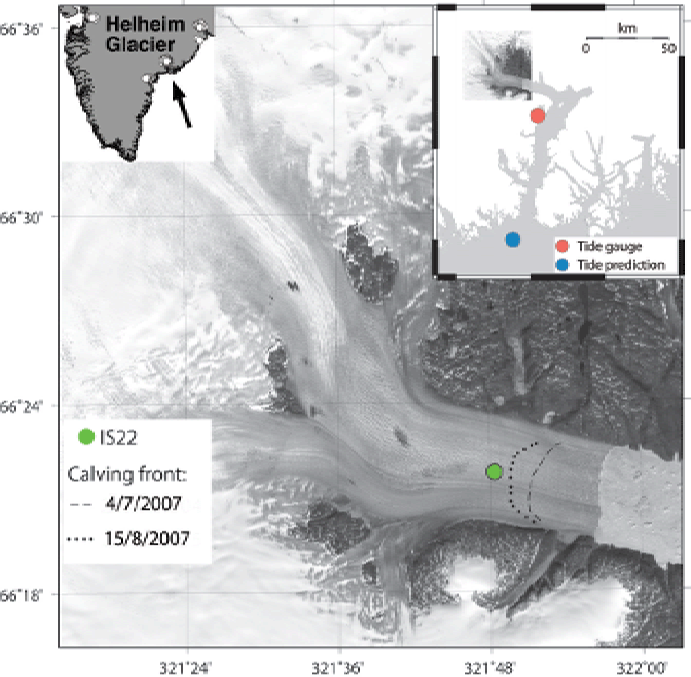
We infer sea level from pressure-gauge observations acquired in a cove off Sermilik Fjord, at a distance of ~35 km from the terminus (Fig. 1) of Helheim Glacier. These data were recorded continuously at 1 min intervals during days 203–220 of year 2006 and 186–218 of 2007. The pressure gauge (hereafter referred to as a ‘tide gauge’) has a nominal resolution of ~1 mm.
Landsat image of Helheim Glacier, southern Greenland, acquired 2001, showing the location of the GPS site IS22. Black dotted and dashed curves show the positions of the calving front at two times (4 July and 15 August) during the summer of 2007. Top left inset: Arrow marks the location of Helheim Glacier in southern Greenland, with white dots showing locations of glacial earthquakes (Reference Tsai and EkströmTsai and Ekström, 2007). Top right inset: Map of the region showing Sermilik Fjord, and locations of the tide gauge and the tide prediction point. (Figure after de Juan and others, 2010.)
We focus on the sea-level time series for 2007 (Fig. 2a). A purely visual inspection indicates that the variations during this period are dominated by a semidiurnal component, modulated at ~15 days. There is also a smaller diurnal component that contributes to the pattern of semidiurnal maxima with alternating large and small amplitudes. This particular pattern persists even when the sinusoidal amplitude is small, due to the 15 day modulation (i.e. at neap tide). Shorter periods of high-frequency variability are observed during and following periods of large calving events associated with glacial earthquakes, as seen around days 189–190 (Reference NettlesNettles and others, 2008).
Sea-level observations from Sermilik Fjord in 2007, along with a comparison with an open-ocean tide model. (a) Blue: observations. A mean value of 2.176 m has been subtracted. Red: AOTIM-5 ocean tide model (Reference Padman and ErofeevaPadman and Erofeeva, 2004) calculated at a location outside Sermilik Fjord (Fig. 1) for days 185–220 in 2007. (b) Observed minus model differences. (Note the different scale.)

The sea-level observations are in close agreement with tidal predictions (red curve in Fig. 2a) from the Arctic tidal model AOTIM-5 (Reference Padman and ErofeevaPadman and Erofeeva, 2004), evaluated for a location in the open ocean just outside Sermilik Fjord (Fig. 1). However, the differences between the observations and model (Fig. 2b) are not negligible. In particular, the differences show harmonic variations with diurnal and semidiurnal periods of maximum amplitude ~0.1 m. Differences between sea-level changes within the fjord and the tide model may be due to atmospheric pressure, winds and runoff within the fjord, all of which can have significant diurnal variability (e.g. Reference Svendsen and ThompsonSvendsen and Thompson, 1978; Reference Mortensen, Lennert, Bendtsen and RysgaardMortensen and others, 2011).
Other differences between the sea-level observations and the tide model can also be observed in Figure 2. The short time spans of high-frequency variations are due to tsunamis produced by calving (Reference NettlesNettles and others, 2008). Longer-period variations can also be observed, particularly an apparent rate change around day 190. The longer-period differences are potentially problematic for such a short time series because they have to be dealt with in any spectral analysis. Although the time span of data collected before day 190 is short, there appears to be a change in the secular drift of the differences at this epoch. We speculate that this may be due to one or more of several possible causes: (1) the pressure-gauge electronics adjusting to environmental conditions; (2) a real long-period variation in sea level caused, for example, by winds and pressure variations; or (3) large wave arrivals associated with the glacial earthquakes on days 189–90 may have caused the instrumental drift to change. Since we are interested in a harmonic analysis rather than longer-period variations, we omit the tide-gauge data before day 190 and refer to the resulting dataset as the ‘truncated’ sea-level time series. The truncated sea-level observations have a slightly smaller root-mean-square difference than the tide model (92 compared to 96 mm).
Geodetic data from Helheim Glacier
We acquired continuous GPS observations (dual-frequency phase and pseudo-range data) at sites near the calving front of Helheim Glacier and rock-based sites near the glacier margins (Reference NettlesNettles and others, 2008). The on-glacier network spanned a distance of up to 37 km behind the calving front. The sites were generally distributed along the glacier’s center flowline, although several sites were established off this line to measure cross-glacier flow variation. All systems employed geodetic-quality, dual-frequency Trimble NetRS or Trimble R7 receivers and Trimble Zephyr antennas. We recorded phase, pseudo-range and other data at sampling intervals of 1–5 s. Our on-glacier networks consisted of 23 sites on the glacier surface in 2006, 16 in 2007 and 23 in 2008.
We used the TRACK software package (Reference ChenChen, 1998) to perform a fully kinematic analysis of the GPS data. This analysis yielded time-dependent estimates of position every 15 s for the GPS antennas on the glacier relative to the static bedrock antennas. Geocentric Cartesian coordinate time series from each day were transformed into glacier-based coordinate systems by a rotation about the local vertical axis to define ‘along-flow’ and ‘cross-flow’ components. Typical formal uncertainties for the horizontal coordinates are 5–10 mm. We deleted position estimates for epochs at which any ambiguities were unresolved.
In 2007, we acquired data from various Helheim Glacier sites from day 185 (4 July) to 237 (25 August) (Reference NettlesNettles and others, 2008). Site IS22, located a distance of 1.3–2.5 km from Helheim Glacier’s terminus near the center of the glacier (Fig. 1) provides a nearly complete time series for 21 days (186–206) in 2007, a period of significant overlap with the tide-gauge record. The glacier was grounded at or near the calving front during the period of observation, based on the lack of a vertical response at this site.
The time series of estimated along-flow position for IS22 from the GPS analysis, after removal of a mean flow of 22.3 m d-1, is shown in Figure 3. Days 189 and 190 have been omitted from this plot and from the analysis below, since these time series are complicated by a series of glacial earthquakes (Reference NettlesNettles and others, 2008; de Juan and others, 2010). Day boundaries are shown to emphasize the fact that the GPS data were analyzed independently in 1 day batches (Reference NettlesNettles and others, 2008; de Juan and others, 2010), as is typical for such data.
Estimated relative along-flow position for GPS site IS22 (Fig. 1). (a) Along-flow position relative to mean flow of 22.3 md−1. (b) Along-flow position relative to a model for long-term variability of position, revealing harmonic variability. Data during the days of glacial earthquakes (189–190) have been omitted.
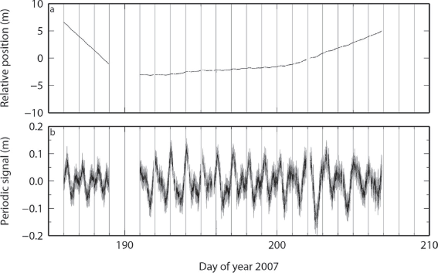
At the scale of Figure 3a, non-periodic variations in velocity are dominant, and periodic variations are barely visible. To view these, we first remove an approximate model for the long-period variability. The resulting variations in flow are shown in Figure 3b. At this scale, the glacier flow can be seen to contain large diurnal and semidiurnal variations of time-dependent amplitude.
Methods
The goal of our study is to understand the source of the observed harmonic variations of glacier flow for Helheim Glacier, a fast-flowing tidewater glacier. As we discussed in the Introduction, previous studies (e.g. Reference Meier and PostMeier and Post, 1987) have demonstrated that such glaciers respond to tidal forcing. A small number of studies (e.g. Reference AndersenAndersen and others, 2010, Reference Andersen, Nettles, Elosegui, Larsen, Hamilton and Stearns2011) have demonstrated that large tidewater glaciers can respond to atmospheric forcing on multi-day timescales. However, it has not been demonstrated that Greenland’s tidewater glaciers respond to diurnal atmospheric forcing. Our approach will therefore be first to explore whether we can fully explain the harmonic variations of Helheim Glacier using a tidal admittance (e.g. Reference O’Neel, Echelmeyer and MotykaO’Neel and others, 2001). We will then use the internal consistency of the results, reflected in the variability of the admittance across the tidal spectrum, to search for the presence of non-tidal components of glacier flow.
Because of the short lengths of the fjord sea-level and glacier-flow time series, it is not possible to determine the complete spectrum of sea-level variations, or to separate closely spaced harmonics uniquely. However, the goal of this study is not to provide such a complete model, but rather to understand the amplitude of variations of the main constituents within the diurnal and semidiurnal bands. Our analysis thus allows for some differentiation among constituents within each band. In addition, we wish to perform the same analysis on both the tide-gauge and position time series, where the latter is dominated by large non-periodic flow-speed variations. Although biases between daily analyses of GPS data of position appear to be small in Figure 3b, we allow for such a possibility in order not to misinterpret such potential biases in terms of harmonic variability. We therefore seek an alternative to the traditional harmonic analysis approach, that will enable simultaneous estimation of the variable flow signal and harmonic components and that will minimize the impact of these biases.
In performing this analysis for the tide-gauge data, we start with components in the harmonic spectrum of AOTIM-5 for the location shown in Figure 1. However, the qualitative analysis based on visual inspection of the differences between the time series and the tide model in the previous section indicated significant differences between sea-level variations in the fjord and those predicted for tides in the open ocean. Given the short time series, we cannot resolve the exact frequency of the differences. The tide model includes components at two nearly diurnal tidal frequencies, i.e. frequencies, f, close to 1 cycle per (solar) day (cpd), but it does not include the S1 tide (f = 1 cpd) because this tide is very small in the open ocean (e.g. Reference Ray and EgbertRay and Egbert, 2004). The P1 tide has a frequency of 1–1/365: 243 cpd and the K1 tide has a frequency of 1 + 1/365: 243 cpd However, due to the possibility of environmental forcings in the fjord that are not present, or are much smaller, in the open ocean (e.g. Reference Svendsen and ThompsonSvendsen and Thompson, 1978; Reference Mortensen, Lennert, Bendtsen and RysgaardMortensen and others, 2011), we allow for the possibility of an S1 component in the fjord sea level.
To estimate components at these close frequencies in the sea-level data, we constrained the ratio of the P1 and K1 amplitudes to their AOTIM-5 values. This is similar to the technique of inference (Reference GodinGodin, 1972), except only the real amplitudes were constrained. Due to the short length of the time series, we made no nodal modulation corrections (e.g. Reference GodinGodin, 1972). Long-period tides could not be determined, and we simply remove a best-fit straight line prior to harmonic analysis.
Given the approach described in the first paragraph of this section, we wish to decompose the glacier-flow time series into harmonic series based on tidal constituents, but we do not wish to constrain the amplitudes based on the estimated model for the sea-level observations. A challenge in the analysis of the glacier-flow data arises because, in comparison with the tide-gauge data, the glacier-flow uncertainties are larger relative to the periodic signals (Fig. 3), and there are also data gaps. The problem of separation of various constituents is thus more acute, especially for the P1, S1 and K1 components. We nevertheless must choose specific frequencies to use for estimation. Therefore, we model any combined diurnal signals that cannot be resolved from one another using a frequency of 1 cpd (i.e. S1).
We used the method described in the Appendix to analyze the sea-level and position time series consistently. The initial step of this approach involves estimating, and removing, amplitudes of signals with nominal frequencies within each band for daily batches of data. (We choose 1 and 2 cpd for simplicity.) This procedure has the effect of shifting downward the frequencies of the components making up the original time series. For example, a signal with the M2 frequency when shifted by 2 cpd has a frequency of –0.0677 cpd (period of –14: 764 days), which can be easily distinguished from a signal with the shifted N2 frequency of –0.104 cpd (period 9.614 days). The S2 component itself shows up in the shifted signal as a zero-frequency offset. The amplitude of each identified harmonic will potentially represent the summation over dozens or hundreds of tidal harmonics that are indistinguishable over so short a time span. We compared results for our code against T_TIDE (Reference ForemanForeman, 1977; Reference Pawlowicz, Beardsley and LentzPawlowicz and others, 2002) using simulated time series, and found good agreement.
Results
Power spectral densities
The estimated power spectral density (PSD) for each observed time series is shown in Figure 4. For the sea-level data, a straightforward Fourier-transform method was used on the truncated time series. For the position time series, we first limited ourselves to the nearly linear span of data from days 191–200. Even during this period there are daily speed variations of 0.1–0.3 md−1, so we first removed a model consisting of best-fit daily piecewise continuous straight lines. To account for unequal data spacing (due to data deletions) and unequal standard deviations, we used the Lomb–Scargle method (Reference LombLomb, 1976; Reference ScargleScargle, 1982) to calculate the PSD.
Power spectral densities of the observed time series, with initial identifications of the spectral peaks. (a) Truncated sea-level series. (b) Power spectral density of along-flow position from GPS, after subtraction of a best-fit model consisting of daily piecewise-continuous straight lines. Diurnal (D) and semidiurnal (S) peaks are labelled. The PSDs are normalized so that integration across the band shown in the plot yields the sample variance.

For each spectrum in Figure 4, an initial identification of spectral peaks is shown. For the sea-level data, the PSD reveals four main peaks, which we nominally identify using Darwin notation. The S1, K1 and P1 components cannot be separated visually in this plot, and the diurnal peak has been labelled ‘K1/P1/S1’. Peaks at 3, 4 and 5 cpd are also visible, which may be present in the open-ocean tide or produced by internal reflections within the fjord (e.g. Reference Valle-Levinson, Blanco and FrangópulosValle-Levinson and others, 2007). Higher-frequency power associated with calving events and, presumably, data noise is also present in the PSD.
For the glacier-flow time series, peaks at diurnal, semidiurnal and other diurnal harmonics are visible. Due to the relatively poor resolution of the flow PSD compared with the sea-level PSD (due to larger errors and data gaps), we have labelled the peaks simply ‘D’ for diurnal and ‘S’ for semidiurnal. In contrast to the tide-gauge spectrum, the glacier-flow spectrum has more energy in the diurnal frequency band than in the semidiurnal.
Harmonic constituents
The results of the harmonic analysis of the sea-level data (Table 1, columns labelled ‘Sea level’) are consistent with the visual inspections of the time series and its PSD, in indicating that sea-level variation is dominated by semi-diurnal tides. The primary harmonic is M2, with an amplitude of ~1.0 m. The next largest component is S2, with an amplitude only 34% of the M2. The root-sum-square (rss) of all the diurnal amplitudes (labelled ‘D’ in Table 1) is 18% of that for the semidiurnal (SD) amplitudes, a result consistent with the visual observation of the primarily semidiurnal nature of the ocean tide (Fig. 2).
Results of the analysis of the truncated sea-level and glacier-flow time series. Rows labelled ‘D’ (diurnal) and ‘SD’ (semidiurnal) give the root-sum-square of the amplitudes for the respective band

The S1 frequency we found for the sea level is too large to be reasonable for the S1 tide in the open ocean (e.g. Reference Ray and EgbertRay and Egbert, 2004), but we cannot say with certainty whether this is a real sea-level variation that occurs within the fjord or whether this represents entanglement with K1 and P1. The S1 ocean tide can reach the centimeter level near Helheim Glacier (Reference Ponchaut, Lyard and le ProvostPonchaut and others, 2001). However, we are not so much concerned with the details of the tidal model in the fjord as the comparison of energy in the diurnal and semidiurnal bands.
The analysis of the glacier-flow time series (Table 1, columns labelled ‘Glacier flow’) produced fewer components, because of the larger uncertainties, relative to the signal, of these data. Two relatively large diurnal components were estimated, although we lack the ability to resolve the closely spaced nearly diurnal signals (see Methods section). In contrast to the sea-level spectrum, the diurnal amplitude for the flow spectrum is larger than the semidiurnal by a factor of ~1.5. We therefore suspect that these components of glacier flow may be primarily non-tidal in origin.
The residuals for both the sea-level and glacier-flow time series, relative to their respective models composed of the harmonic components of Table 1 (along with the long-term trend variations), are shown in Figure 5. The rms residual for the sea-level data is 42 mm, indicating, as might be expected for an analysis based on a short record, a much closer agreement of this model with the sea-level observations than achieved by the open-ocean tide model. The residuals do not appear to contain any harmonic variability that is coherent over the time span of the data. We did not estimate any higher-order harmonics, so those would still be present in the residuals. However, there is no obvious pattern in the residuals that would modify our conclusion that the sea-level variability in the fjord is dominated by the semidiurnal components of the ocean tide. We note that, due to the short time span of the tide-gauge time series, these results do not represent a complete tidal model in the sense of, for example, AOTIM.
Residuals relative to the best-fit sea-level and glacier-flow models. (a) Tide-gauge residuals. The rms residual is 42 mm. (b) Glacier-flow residuals. The rms residual is 20 mm.

The rms residual for the glacier flow (Fig. 5b) is 20 mm. While this fit is better than that for the sea-level data in absolute terms, relative to the amplitude of the signal it is worse. The signal-to-noise ratio is ~25 for the sea-level data, ~2.8 for the glacier-flow data. These results are not surprising given the much larger uncertainties of the position estimates compared with the nominal tide-gauge uncertainties. However, the residuals from both time series show systematic variations. For sea level, ocean-dynamic signals play an important role. For the glacier-flow data, the systematic variations at short periods are more pronounced, and the residuals (Fig. 5) are on the same order as the estimated amplitudes (Table 1). The model fit is especially poor around day 203.
Analysis
One way to compare the spectra of the ocean tide and the periodic glacier flow is to model the glacier-flow variations for the k th harmonic component, xk (t), as a lagged linear response to sea-level forcing, Fk :

where Ak is the admittance and τk the time delay for the k th harmonic component (Reference Walters and DunlapWalters and Dunlap, 1987; Reference O’Neel, Echelmeyer and MotykaO’Neel and others, 2001). Our estimates of the admittances and delays are shown in the last two columns of Table 1. We calculated the admittance by dividing the along-track flow amplitude by the ocean-tide amplitude. A negative sign for the admittance indicates that a positive sea-level change yields a negative flow displacement. The lag, τk , for the k th harmonic component is calculated from the phase (°) using

where  is the tide-gauge phase, is the along-track flow phase, Tk
is the period (hours) and the quantity in parentheses is taken modulo 360°. The 180° phase advance takes into account the fact that, for sea-level back-pressure forcing, the along-track position minima occur near forcing maxima (e.g. de Juan and others, 2010).
is the tide-gauge phase, is the along-track flow phase, Tk
is the period (hours) and the quantity in parentheses is taken modulo 360°. The 180° phase advance takes into account the fact that, for sea-level back-pressure forcing, the along-track position minima occur near forcing maxima (e.g. de Juan and others, 2010).
Can we assume a frequency-independent response of the glacier back-pressure forcing? In many models, glacier speed is proportional to the driving stress, τn , with n ≃ 3 (e.g. Reference WaltersWalters, 1989; Reference PatersonPaterson, 1994; Reference Howat, Joughin, Tulaczyk and GogineniHowat and others, 2005). For ice streams with small mean driving stresses and large tidally imparted hydrostatic stresses, this nonlinearity yields tidal flow responses that are unequal across tidal frequencies (e.g. Reference GudmundssonGudmundsson, 2007; Reference King, Watson, Penna and ClarkeKing and others, 2010). However, in glaciers for which the tidally imparted stress is small compared with the mean driving stress (e.g. Helheim Glacier), these models predict a linear response to the tide. Using the model described by Reference GudmundssonGudmundsson (2007), we find that the term that has a linear dependence with tidal height is at least two orders of magnitude larger than higher-order, nonlinear terms.
The mean semidiurnal admittance (Table 1) is –0. 028 ± 0. 002. Applying this admittance to the diurnal components, it is not surprising that no position spectral components for P1, K1, K2, ν 2 and O1 appear, since their amplitudes in the tide-gauge spectrum are too small. The admittances for the M2, S2 and N2 components are consistent at better than the 2σ level, whereas the admittance for the S1 component is a factor of ~27 larger, and that for the Q1 component is ~36 times larger. The phases of the position spectra reveal a time lag of position relative to the tide-gauge observations. Again, the M2, S2 and N2 lags are consistent, and within 2σ of the weighted mean of 1.9 hours. However, the S1 lag is 21.7 hours and the Q1 lag is 11 hours.
Figure 6 demonstrates that the three primary observed semidiurnal components (M2, S2 and N2) of the along-track glacier motion at site IS22 can be accurately predicted from the tide-gauge observations, using a single admittance and response lag. The two primary diurnal components (S1 and Q1), however, cannot be predicted from these same admittance and lag values; in fact they cannot be predicted from any single pair of admittance and lag. As we argue above, the response of Helheim Glacier to sea-level back-pressure forcing should vary little, if at all, between diurnal and semidiurnal bands, in which case all the admittances and lags should be equal, whereas our results require a large difference in the responses between the diurnal and semidiurnal bands.
Phasor diagram of the IS22 position spectral components (blue), along with predictions (red) based on the tide-gauge spectra using the mean semidiurnal admittance and lag from Table 1. The 95% confidence ellipses are shown. The P1, K1, K2, O1 and ν 2 components are not shown, since no corresponding component for the glacier position was estimated. The Q1 tide-gauge estimate is not shown since it is nearly zero. The predicted M2, N2 and S2 components lie within the 95% confidence ellipses for their respective observed values, whereas those for the S1 and Q1 components do not. Phase angle is measured clockwise from the horizontal x –axis (not shown).

Our analyses of the sea-level forcing and the glacier response lead us to conclude that the diurnal-band glacier motion is largely not a response to back pressure caused by sea-level variation. Based on previous studies of other types of glacier (e.g. Reference Walters and DunlapWalters and Dunlap, 1987; Reference Kamb, Engelhardt, Fahnestock, Humphrey, Meier and StoneKamb and others, 1994; Reference O’Neel, Echelmeyer and MotykaO’Neel and others, 2001) we hypothesize that the diurnal variations in glacier flow are associated with variations in lubrication of the glacier bed, due to surface melting driven by diurnal solar heating. In this scenario, the estimated Q1 harmonic is an artifact that, for our data span, absorbs some of the (possibly weather-dependent) temporal variability of the diurnal signal.
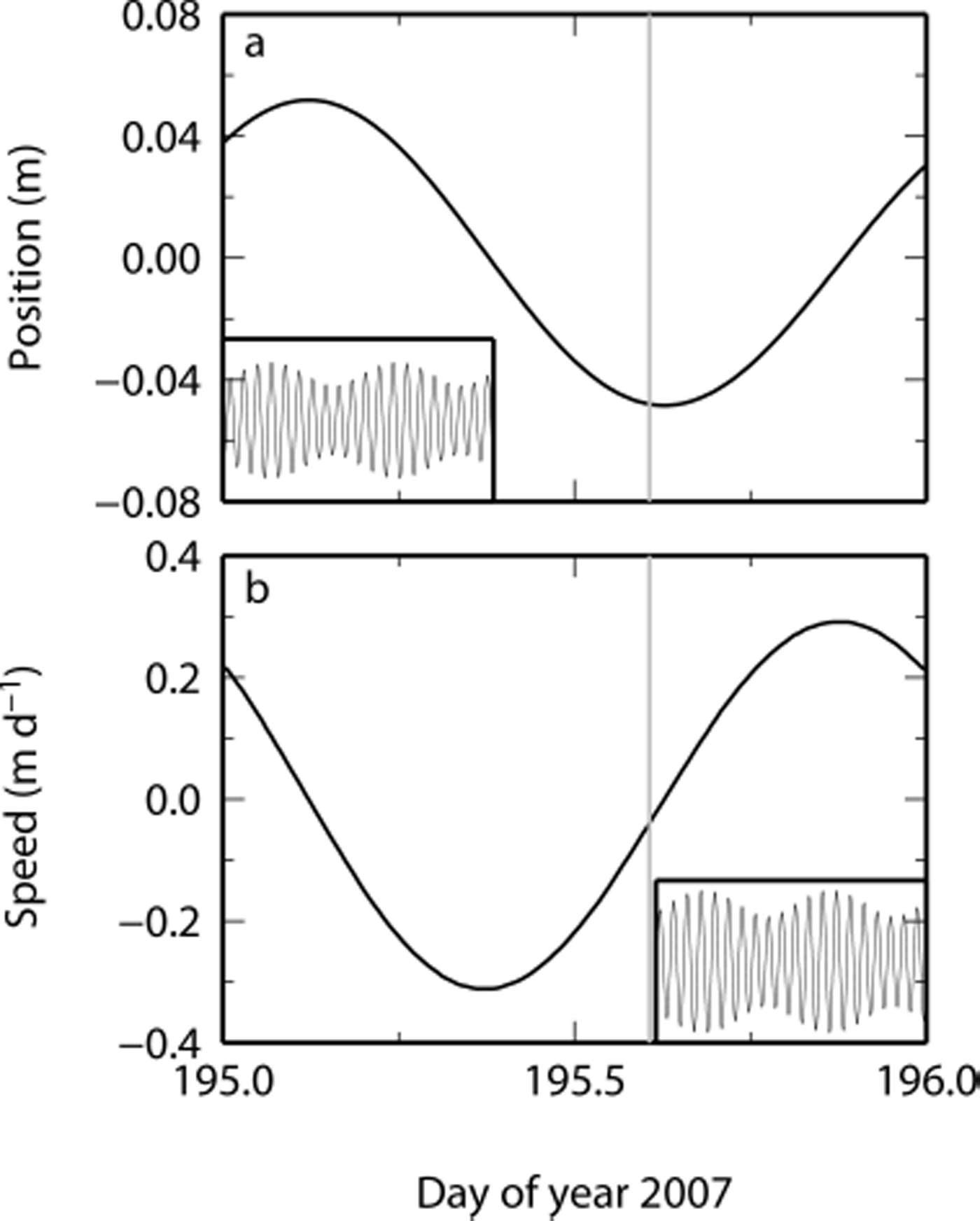
Although separation of tidal and non-tidal components of forcing has previously been challenging (e.g. Reference WalterWalter and others, 2012), we can use the admittances for this purpose. We first formed a residual diurnal position spectrum (as described by Reference O’Neel, Echelmeyer and MotykaO’Neel and others, 2001). We predict the diurnal spectrum of along-flow position using the diurnal sea-level spectrum and mean admittance and lag from Table 1, for the set of diurnal tides estimated for position, also given in Table 1. We then subtract the predicted diurnal spectrum from the observed along-flow diurnal spectrum to obtain the non-tidal variations. One-day model time series for position and velocity formed from the residual non-tidal diurnal components are shown in Figure 7. This signal consists of two components: S1 (with an exactly 1 day period) and Q1, with which the mixing produces the 9.4 day beating period of Figure 7. The ~60 mm position amplitude of this signal produces, in velocity, a speed change of ~0.7 m d-1 amplitude peak-to-peak, or a peak-to-peak variation of ~3% compared with the glacier mean flow speed of ~22 m d-1 at IS22 during this period. From Figure 7, the maximum speed occurs ~6 hours after local noon during this period and varies slightly over a longer time period because of the Q1 modulation. (The insets of Fig. 7 show longer time spans.)
Model for the non-tidal diurnal signal in IS22 along-flow position and speed predicted from the residual glacier-flow spectrum, for day 195. The solid gray line indicates local noon based on the longitude of Helheim Glacier. Insets: model time series for days 190–210.
In their investigation of speed variations at Columbia Glacier, Alaska, Reference Walters and DunlapWalters and Dunlap (1987) found that a component of the variations was correlated with solar insolation, which they used as a proxy for melt runoff. They found a lag of ~8 hours between the glacier speed response and the insolation. We find that the maximum glacier speed from the non-tidal signal occurs ~6 hours past local noon; a good agreement with Reference Walters and DunlapWalters and Dunlap (1987), if we assume that solar altitude should also be a good proxy for melt. However, Reference Walters and DunlapWalters and Dunlap (1987) found their melt signal to be temporally variable, a reasonable finding given that insolation at the surface is impacted by weather. The analysis presented above, which was focused on the tidal spectrum, estimated a single S1 amplitude and phase for the entire position time series. Visual inspection of the postfit residuals (Fig. 5), however, leads us to infer that a temporally variable diurnal signal might be more appropriate. The postfit residuals have some periodicity. In the earlier half of the time series, there is a clear residual diurnal variation, and the model is unable to reproduce the variability during some days (e.g. days 201–203).
To investigate the variability of the diurnal component further, we designed a Kalman filter (e.g. Reference Ravishanker and DeyRavishanker and Dey, 2002) to estimate the parameters of an admittance model with a stochastic (random-walk) along-flow speed, tidal admittance, tidal-response lag and amplitude of the diurnal sinusoidal variability. The model for the along-flow position, x (t), is given by

Here x˳ = x(t ˳)is the position at initial epoch t˳ v (t) is the non-periodic along-flow speed, A (t) is the tidal admittance, F (t) is the tide-gauge observation, τ (t) is the lag, (t) is assumed to be zero-mean Gaussian random error and the diurnal signal, x D(t), is given by

This form was used to insure continuity across day boundaries, at which epochs the contribution of x D(t) is identically zero. The stochastic amplitudes, a c(t) and a s(t), were modeled as slowly varying random-walk stochastic processes with variance rates of 10-4 m2 d-1. For this analysis, only data from the period when the GPS observations overlapped with the tide-gauge observations were used, and observations during the glacial earthquakes were retained to provide continuity.
The results of the Kalman-filter solution are shown in Figure 8. Figure 8a shows the diurnal contribution of Eqn (4). During this time span, the amplitude of the diurnal signal varies by a factor of ~2. The most rapid change is seen in days 189–190, during the period of glacial earthquake activity. Reference De JuanDe Juan and others (2010) reported an abrupt change in the tidal admittance during that time, that we also find. The postfit residuals shown in Figure 8b are significantly smaller than those calculated using the model with a constant diurnal amplitude (Fig. 3b), having an rms value less than half that of the previous solution.
Results from the Kalman-filter solution with stochastic S1 amplitude. (a) Estimated S1 contribution (x D(t) from Eqn (4)). (b) Postfit residual. The rms residual is 9.7 mm. Error bars (1) are shown in gray.
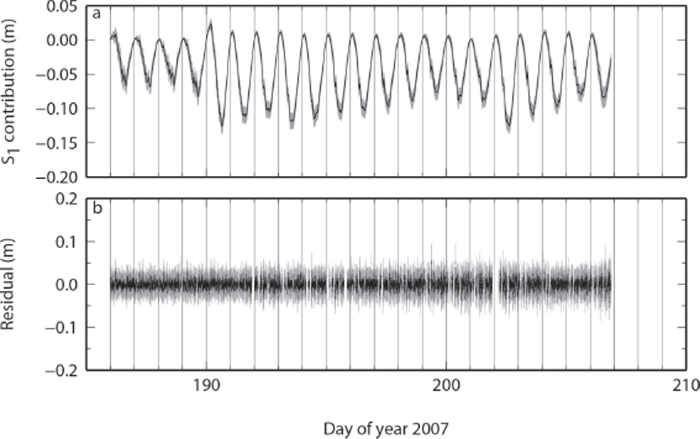
The Kalman-filter solution explicitly includes only those harmonic components inherent in the tide-gauge data (and having the same relative amplitude as in the tide-gauge data) plus an additional time-variable diurnal component. The time variability of a diurnal component will express itself (in power-spectrum terms) as a broadening of the peak centered on the diurnal frequency. The ability of the stochastic model to fit this variability reinforces the supposition, discussed above, that the large Q1 component was simply an artifact of that variability over this short time series.
In future studies, we plan to use meteorological data collected on Helheim Glacier to improve our understanding of the influence of melt on glacier flow. We have previously been able to model the surface energy balance with some accuracy (Reference AndersenAndersen and others, 2010, Reference Andersen, Nettles, Elosegui, Larsen, Hamilton and Stearns2011), and comparison with a more complete analysis of speed variations throughout the network should be fruitful. Although such a study is beyond the scope of this paper, we can perform a simple comparison of the model for speed variations inferred from the Kalman-filter model for the diurnal contribution with measurements of temperature obtained at the nearby weather station at Tasiilaq (Fig. 9). The speed and temperature variations are clearly correlated, with the speed generally lagging the temperature by ~3.8 hours. The temporal variability of the amplitude response shows a more complex relation, as expected from previous work at Columbia Glacier (e.g. Reference Kamb, Engelhardt, Fahnestock, Humphrey, Meier and StoneKamb and others, 1994).
Comparison of estimated diurnal speed variations for IS22 from the Kalman-filter (blue) and surface air temperature anomalies from the nearby weather station at Tasiilaq (red) relative to a Gaussian smoothed value calculated with a 1.5 hour window. Data from Reference CappelenCappelen (2014).

We have focused on GPS site IS22 for this study because it provides a complete, high-quality record of flow variations during a period in which tide-gauge observations were also available, and the goal of this study was to identify and quantify the non-tidal component of glacier flow. Interpretation of our previous analyses (de Juan and others, 2010), in light of the results presented here, leads us to expect that future study of a broader range of glacier sites and of longer time periods may prove illuminating.
Conclusions
We compared the spectrum of sea-level time series acquired in Sermilik Fjord near Helheim Glacier with the spectrum of along-flow position time series acquired from a GPS site on the glacier. We found that the position spectrum was poorly explained by the assumption of forcing by the sea level alone, and that there were additional components to the motion in the diurnal band, centered around the S1 frequency of 1 cpd The non-tidal variations accounted for a peak-to-peak variation in glacier flow speed of ~0.7 m d-1 at a location where the mean flow rate was ~22 m d-1. The phase of the non-tidal variations was such that the maximum flow speed was reached ~6 hours after local noon, suggesting that the source of these variations was surface runoff from ice melt associated with solar heating. Further investigation of the non-tidal diurnal signal using a stochastic filter revealed that it could be better modeled using stochastic amplitudes (sine and cosine) that varied by a factor of ~2 over the ~21 day dataset.
Our analysis focused on rigorously establishing the presence of non-tidal diurnal variations in glacier speed. It is reasonable to conclude that the non-tidal signal is associated with melt runoff, both from the point of view of the above discussion and what is known regarding the influence of runoff on glacier flow. At periods exceeding 1 day, data from Helheim Glacier have already been used to investigate the relationship between flow-speed variations and melt (Reference AndersenAndersen and others, 2010, Reference Andersen, Nettles, Elosegui, Larsen, Hamilton and Stearns2011). However, unambiguous identification of a non-tidal melt component at timescales of ≤ 1 day is not straightforward. Any melt component associated with solar heating will be represented mainly at a frequency of 1 cpd and harmonics thereof, which are also valid tidal frequencies. Moreover, the melt component will maintain phase with these tides, since the Sun is the main contributor to both forcings. In our case, we were able to compare the spectrum of glacier-flow determinations from GPS to the tide spectrum from tide-gauge observations. Our approach also depends on having highly accurate continuous time series, such as those afforded by geodesy with GPS.
Our comparison of the spectra of the tidal forcing and glacier flow yielded tidal admittances in good agreement with the admittances calculated by de Juan and others (2010) using a purely time-domain modeling approach. This agreement is due both to the large semidiurnal component of the tidal forcing and also to the inclusion by de Juan and others (2010) of an additional acceleration parameter that absorbed much of the variable diurnal signal reported here. Our work suggests that a comparison of the spectra of the various forcings and the glacier flow are important to understanding their individual contributions.
Acknowledgements
We thank members of the Helheim Project for collecting the datasets used in this analysis. This work was supported by US National Science Foundation grants ARC-0713970, ARC-07131749 and ARC-1110322, the Gary Comer Science and Education Foundation, the Spanish Ministry of Science and Innovation (MICINN; now MINECO), the Danish Commission for Scientific Research in Greenland (KVUG), the Geological Survey of Denmark and Greenland (GEUS), Geocenter Copenhagen, the Danish National Space Center and NASA. GPS equipment and technical support were provided by UNAVCO, Inc. We thank H. Fricker, L. Padman (who suggested use of the inference method) and an anonymous reviewer for constructive reviews, and R. Ray for useful discussions.
Appendix
A tidal signal, T(t), can be represented as

The superscripts in Eqn (A1) represent the tidal band: (1) for diurnal, (2) for semidiurnal, etc.; T L are the long-period tides, which we hereafter ignore. The summation in each band is carried out over the large number of tidal constituents that make up that part of the tidal spectrum.
The phase angle,  , is a summation of astronomical angles (e.g. Reference Petit and LuzumPetit and Luzum, 2010) that we express in radians as

Here  is the angle of the S
n
tide, t
’ is the fraction (0 ≤ t
’ < 1) of the day corresponding to t, which is typically the time in Julian centuries of 36 525 days since the reference epoch, J2000.0 (1.5 January 2000), and f˳ = 1 cpd. Equation (A2) defines
is the angle of the S
n
tide, t
’ is the fraction (0 ≤ t
’ < 1) of the day corresponding to t, which is typically the time in Julian centuries of 36 525 days since the reference epoch, J2000.0 (1.5 January 2000), and f˳ = 1 cpd. Equation (A2) defines  . The first term on the right-hand side of Eqn (A2) varies much more rapidly than
  , which varies (for n = 1 and 2) at a rate of ≤ 13° d-1. Because
  is more slowly varying, it can be expanded on any particular day to first order in Δt = t – tm
, where tm
is the epoch at noon as
is more slowly varying, it can be expanded on any particular day to first order in Δt = t – tm
, where tm
is the epoch at noon as

where  is in cycles per day and
  is the tidal frequency for the i th constituent of the n th tidal band. The error in this approximation, for the tidal constituents of Table 1, evaluated for t = 0.1 (~2010.0), is <10−8 cycles.
Using the approximation in Eqn (A3), the tide for the n th band can be approximated as

The cosine in Eqn (A4) can be expanded to yield
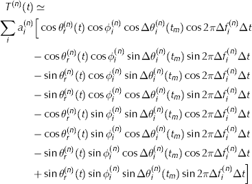
In Eqn (A5),  varies with a diurnal (for the diurnal band) or semidiurnal (for the semidiurnal band) period, but is the same for all the constituents represented by the index i in the n th band. The phase
  is constant in time, and
  is constant for the day. The phase
  is small but not negligible. For the tidal frequencies in this paper, that term for|Δt| ≤ 0.5 day is ≤0.17 rad ≃10°. Expanding the sinusoids in this term to first order therefore introduces an error in an individual component of <6% of . (In principle, one could perform this expansion to second order and estimate coefficients to quadratic variations in Δt. The error introduced in this expansion would then be reduced to <1% of.
Expanding the trigonometric terms of Eqn (A5) to first order in  and regrouping we get

with

Equations (A6) and (A7) suggest a two-step process (e.g. Reference Mitrovica, Davis, Mathews and ShapiroMitrovica and others, 1994) for estimation of the tidal spectrum, meaning the unknown amplitudes  and phases
  . In the first step, Eqn (A6) is used to model the tidal variation within each tidal band (diurnal, semidiurnal) during 1 day. Thus, for each day, eight parameters are estimated: two amplitudes, A
(n)(tm
) and B
(n)(tm
), and two amplitude rates, C
(n)(tm
) and D
(n)(tm
), for each of the tidal bands. The estimation procedure should also produce an 8 × 8 covariance matrix for the estimated parameters that is used in the next step.
. In the first step, Eqn (A6) is used to model the tidal variation within each tidal band (diurnal, semidiurnal) during 1 day. Thus, for each day, eight parameters are estimated: two amplitudes, A
(n)(tm
) and B
(n)(tm
), and two amplitude rates, C
(n)(tm
) and D
(n)(tm
), for each of the tidal bands. The estimation procedure should also produce an 8 × 8 covariance matrix for the estimated parameters that is used in the next step.
In the second step, the set of estimated parameters from a series of days are treated as data with Eqn (A7) being the observation equations. To linearize this step, we let  , so that Eqn (A7) becomes

Equations (A8) can be used to calculate the partial derivatives, and the parameters  and
and  for each band for a suitable set of tidal frequencies are thereby estimated. The tidal amplitudes and phases are

For some harmonics, the signs in Eqn (A9) must be changed for consistency with convention. The i th contribution to the summation in Eqn (A8) varies sinusoidally with a frequency of  and, therefore, with a period,
  , of
, of

For example, in the semidiurnal band, the M2 tide has a frequency of ~1.9322736 cpd The reference tide for the semidiurnal band, S2, has a frequency of 2 cpd. The semidiurnal amplitudes estimated from the first step would then vary with a period of ~14.7653 days. This two-step approach is most useful when the time series result from independent daily analyses, i.e. when the time series is not long enough to estimate a full spectrum of tidal components directly. (However, Reference Yuan, Chao, Ding and ZhongYuan and others (2013), have shown that if the entire time span is long enough, even sets of a highly correlated tidal amplitude parameters estimated from daily data can be separated adequately.) It enables visual identification of the main spectral components even from fairly short time series. Figure 10 shows estimates of the diurnal and semidiurnal amplitudes from the first step in the process. The large mean (i.e. zero-frequency) offset in the diurnal amplitudes reveals a large S 1 component. The 9 day sinusoidal variation is indicative of the Q1 tide. For the semi-diurnal band, the zero-frequency offset (indicating the S2 tide) is quite small, and the variations are dominated by a ~14 day periodicity, indicating the M2 tide. The amplitude of these tides can be estimated using Eqn (A8), the postfit residuals formed, and then the process can be repeated for identification of progressively smaller amplitude corrections, as well as for tides of smaller amplitudes.
Example plots of the amplitudes for the diurnal (A (1)(tm ) and B (1)(tm ) from Eqn (A6)) and semidiurnal (A (2)(tm ) and B (2)(tm )) terms as a function of tm for site IS22. The gray curves indicate the final spectral model after fitting the amplitudes to Eqn (A8).


 Open access

