


Impact Statement
The blood flow pattern in the heart is an important indicator of cardiac health. Several flow-derived metrics have been proposed to evaluate cardiac diseases; however, their translation to clinical practice has proven difficult due in part to their flow resolution requirements, computational cost and non-intuitiveness. By constructing braids from the entanglements of a modest number of particle trajectories, we readily derive topological properties that characterize cardiovascular flows in an intuitive, global and computationally practical manner. These properties uniquely describe the mixing characteristics of the flow pattern such as its swirling direction and strength, as well as its mixing effectiveness. The braid approach suggests a clinically practical alternative that can be easily implemented on current clinical machines.
1. Introduction
Our hearts are home to some remarkable fluid dynamics. In health, each cardiac chamber fills by way of elegant swirling patterns that facilitate the ensuing ejection of blood (Reference Kilner, Yang, Wilkes, Mohiaddin, Firmin and YacoubKilner et al., 2000). With evolutionary pressures shaping our complex anatomy, it is natural to suspect that these healthy flow patterns have been selected for based on specific driving factors. Cardiac diseases would then have the tendency to distort and deteriorate these patterns, rendering them unfavourable by some specific measures.
The flow pattern in the healthy left ventricle is a prime example. We illustrate the general fluid motion in figure 1. When the heart muscle relaxes, the left ventricle begins to fill rapidly through the mitral valve. This generates a vortex that persists throughout the cardiac cycle, acting as the organizing centre of the flow and as a reservoir of kinetic energy (Reference Kilner, Yang, Wilkes, Mohiaddin, Firmin and YacoubKilner et al., 2000; Reference Pedrizzetti and DomenichiniPedrizzetti & Domenichini, 2005; Reference Wieting and StriplingWieting & Stripling, 1984). The vortex encourages ‘new’ inflowing blood to closely follow the contour of the ventricle wall, forming a channel from inflow to outflow (Reference Charonko, Kumar, Stewart, Little and VlachosCharonko, Kumar, Stewart, Little & Vlachos, 2013; Reference Di Labbio, Vétel and KademDi Labbio, Vétel, & Kadem, 2018; Reference Hendabadi, Bermejo, Benito, Yotti, Fernández-Avilés, del Álamo and ShaddenHendabadi et al., 2013). Meanwhile, by the end of the filling phase (diastole), ‘old’ blood is organized into a column just below the aortic valve, in position to be ejected with ease (Reference Di Labbio, Vétel and KademDi Labbio et al., 2018). In what sense, then, is this swirling left ventricular flow favourable?
Schematic of blood transport in the healthy human left ventricle as suggested by our previous in vitro experiments (Reference Di Labbio, Vétel and KademDi Labbio et al., 2018) and the in vivo results of Reference Charonko, Kumar, Stewart, Little and VlachosCharonko et al. (Reference Charonko, Kumar, Stewart, Little and Vlachos2013) and Reference Hendabadi, Bermejo, Benito, Yotti, Fernández-Avilés, del Álamo and ShaddenHendabadi et al. (Reference Hendabadi, Bermejo, Benito, Yotti, Fernández-Avilés, del Álamo and Shadden2013). The left ventricle just before diastole is shown in (a) with ‘old’ and ‘new’ blood respectively marked by dark and light shades of grey. (b) Blood flowing into the left ventricle induces a vortex ring to form which entrains fluid already present in the ventricle. (c) The part of the vortex ring adjacent to the ventricle wall largely dissipates while the other end is permitted to propagate further down toward the ventricle apex, forming a channel for incoming fluid along the ventricle wall. ( $d\text{--}h$) The cardiac vortex makes its way to the ventricle centre, encouraging ‘new’ fluid to continue propagating up the ventricle wall and ‘old’ fluid to organize or ‘unravel’ into a fluid column that is readily ejected. Here, and in the following figures, AV denotes aortic valve and MV mitral valve.

The current consensus is that the flow has adapted to diminish the dissipation of energy while promoting the turnover of ‘new’ blood and the washout of ‘old’ blood (Reference Wieting and StriplingWieting & Stripling, 1984); for a thorough review of the left ventricular fluid mechanics literature, refer to Reference Pedrizzetti and DomenichiniPedrizzetti and Domenichini (Reference Pedrizzetti and Domenichini2015). Energy losses would otherwise quickly accumulate from one heart beat to the next, requiring more energy from the heart muscle to compensate. Additionally, stagnant blood would not only impede oxygen and nutrient transport but also increase the likelihood of blood clot formation under adverse conditions. Essentially, the left ventricle possesses characteristics that we associate with a good laminar chaotic fluid mixer (Reference ArefAref, 1984; Reference Aref, Blake, Budišić, Cardoso, Cartwright, Clercx and TuvalAref et al., 2017). It is therefore important to adopt concepts from the fluid mixing literature and explore their application to left ventricular flows. In so doing, we show that the flow in a healthy left ventricle model is favourable according to certain physical measures of mixing.
The canonical experiments of laminar chaotic fluid mixing are those of embedded stirrers following prescribed motion protocols within a circular container (Reference Boyland, Aref and StremlerBoyland, Aref, & Stremler, 2000; Reference Thiffeault and FinnThiffeault & Finn, 2006). By following the two-dimensional motion of the stirrers in time (i.e. in a third dimension), their ‘world lines’ become entangled, forming a braid (Reference ArtinArtin, 1947). Likewise, for more general two-dimensional flows, a braid can be formed by advecting or tracking particles directly and using their trajectories in two-dimensional space and time as the strands of the braid (Reference Allshouse and ThiffeaultAllshouse & Thiffeault, 2012; Reference Boyland, Stremler and ArefBoyland, Stremler, & Aref, 2003; Reference Filippi, Budišić, Allshouse, Atis, Thiffeault and PeacockFilippi et al., 2020; Reference Francois, Xia, Punzmann, Faber and ShatsFrancois, Xia, Punzmann, Faber & Shats, 2016; Reference Gouillart, Finn and ThiffeaultGouillart, Finn, & Thiffeault, 2006; Reference Puckett, Lechenault, Daniels and ThiffeaultPuckett, Lechenault, Daniels, & Thiffeault, 2012; Reference Smith and WarrierSmith & Warrier, 2016; Reference Taylor and Llewellyn SmithTaylor & Llewellyn Smith, 2016; Reference ThiffeaultThiffeault, 2005, Reference Thiffeault2010; Reference Thiffeault and FinnThiffeault & Finn, 2006; Reference Thiffeault, Finn, Gouillart and HallThiffeault, Finn, Gouillart, & Hall, 2008; Reference Yeung, Cohen-Steiner and DesbrunYeung, Cohen-Steiner, & Desbrun, 2020). We illustrate how particle trajectories can be used to produce a braid in figure 2. The properties of the braid then provide global information about the topology of the flow and hence about the quality of the underlying mixing process.
(a) Schematic of four coloured particles (green, red, white and blue labelled  $g$,
$g$,  $r$,
$r$,  $w$ and $b$, respectively) moving in a two-dimensional flow. (b) The corresponding world lines of the particles (the vertical axis being time, $t$) forming a physical braid. (c) The associated braid diagram with time again increasing from bottom to top. The corresponding ‘braid word’ is $\sigma _2\sigma _1^{-1}\sigma _2$, where here we use the convention that a braid word read from left to right represents the braid from bottom to top (i.e. forward in time), and that $\sigma_i$ denotes a clockwise interchange between particles $i$ and $i+1$ whereas $\sigma_i^{-1}$ denotes a counter-clockwise interchange. The ‘length’ of the braid corresponds to the number of crossings in the braid diagram or, alternatively, to the absolute sum of the exponents in the braid word (i.e. $L = |1| + |-1| + |1| = 3$). The ‘writhe’ of the braid, on the other hand, simply corresponds to the sum of the exponents in the braid word (i.e. ${Wr} = 1 - 1 + 1 = 1$).

Strictly speaking, braid theory can only be applied in the context of two-dimensional flows. Cardiovascular flows are inherently three-dimensional and, despite the attention often being limited to two-dimensional slices in clinical practice, the application of braid theory to such flows appears to be disqualifying. The three-dimensional nature of these flows is undoubtedly important, however, there are indeed situations in which the most pertinent three-dimensional features of cardiovascular flows are well represented within specific planes. It is in such situations that braids are useful to cardiovascular flows, namely, when a two-dimensional slice can act as an adequate low-dimensional model due to the representative flow physics it captures. The flow in the healthy left ventricle remains a good example. The three-dimensional flow has been investigated by several research groups, mainly through numerical simulation (Reference Badas, Domenichini and QuerzoliBadas, Domenichini, & Querzoli, 2017; Reference Khalavfand, Xu, Westenberg, Gijsen and KenjeresKhalavfand, Xu, Westenberg, Gijsen & Kenjeres, 2019; Reference Lantz, Bäck, Carlhäll, Bolger, Persson, Karlsson and EbbersLantz et al., 2021; Reference Lantz, Henriksson, Persson, Karlsson and EbbersLantz, Henriksson, Persson, Karlsson & Ebbers, 2016; Reference Mangual, Kraigher-Krainer, De Luca, Toncelli, Shah, Solomon and PedrizzettiMangual et al., 2013; Reference Meschini, de Tullio, Querzoli and VerziccoMeschini, de Tullio, Querzoli, & Verzicco, 2018; Reference Pedrizzetti and DomenichiniPedrizzetti & Domenichini, 2005; Reference Sacco, Paun, Lehmkuhl, Iles, Iaizzo, Houzeaux and Aguado-SierraSacco et al., 2018; Reference Seo and MittalSeo & Mittal, 2013) but also through in vivo (Reference Callaghan, Burkhardt, Valsangiacomo Buechel, Kellenberger and GeigerCallaghan, Burkhardt, Valsangiacomo Buechel, Kellenberger & Geiger, 2021; Reference Costello, Qadri, Price, Papapostolou, Thompson, Hare and TaylorCostello et al., 2018; Reference Eriksson, Bolger, Ebbers and CarlhällEriksson, Bolger, Ebbers, & Carlhäll, 2013; Reference Voorneveld, Saaid, Schinkel, Radeljic, Lippe, Gijsen and BoschVoorneveld et al., 2020) and in vitro (Reference Fortini, Querzoli, Espa and CenedeseFortini, Querzoli, Espa, & Cenedese, 2013; Reference Saaid, Voorneveld, Schinkel, Westenberg, Gijsen, Segers and ClaessensSaaid et al., 2019) studies. While these studies have highlighted the value of the full three-dimensional flow, the observed large-scale dynamics still consists of a global swirling motion that is well captured by the plane shown in figures 1 and 3, namely, one bisecting the valve centres and the ventricle apex. The particle trajectories, which are predominantly influenced by the larger-scale dynamics, appear to be quasi-two-dimensional in the vicinity of this plane (Reference Badas, Domenichini and QuerzoliBadas et al., 2017; Reference Callaghan, Burkhardt, Valsangiacomo Buechel, Kellenberger and GeigerCallaghan et al., 2021; Reference Eriksson, Bolger, Ebbers and CarlhällEriksson et al., 2013; Reference Seo and MittalSeo & Mittal, 2013). Furthermore, several quantitative and qualitative physical features important to particle trajectories (e.g. out-of-plane vorticity, particle residence time, finite-time Lyapunov exponent ridges) captured within this plane (Reference Di Labbio and KademDi Labbio & Kadem, 2018; Reference Di Labbio, Vétel and KademDi Labbio et al., 2018; Reference Domenichini, Querzoli, Cenedese and PedrizzettiDomenichini, Querzoli, Cenedese, & Pedrizzetti, 2007; Reference Espa, Badas, Fortini, Querzoli and CenedeseEspa, Badas, Fortini, Querzoli & Cenedese, 2012; Reference Hendabadi, Bermejo, Benito, Yotti, Fernández-Avilés, del Álamo and ShaddenHendabadi et al., 2013; Reference Okafor, Raghav, Condado, Midha, Kumar and YoganathanOkafor et al., 2017) agree with what has been observed in the cited three-dimensional studies. This does not suggest that the full three-dimensional flow can be entirely disregarded, but rather that this plane can act as a good proxy and, therefore, that the properties of the constructed braids will provide essential mixing information that are at least suggestive of what may be observed in the full flow field. Nonetheless, the use of a two-dimensional description is an important limitation when studying any three-dimensional flow. Specifically, out-of-plane fluid motion can cause true particle trajectories (or their projection onto the plane of interest) to deviate significantly from their in-plane approximations. Out-of-plane fluid motion theoretically negates the applicability of braid theory to the particle trajectories, and in the case of a projection the constructed braid can change significantly. In general, the mixing complexity is expected to increase when considering the full three-dimensional character. Therefore, when using the braid approach on two-dimensional slices of three-dimensional flows, one should at best consider that the computed topological quantities represent a lower bound.
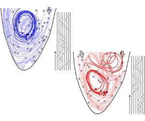
Advection of  $\textit{50}$ virtual particles throughout diastole in (a) a healthy left ventricular flow and (b) one with a severe valvular disease (aortic valve regurgitation). The solid circles represent the positions of the particles at the start of the advection (i.e. at the start of diastole). A select few particle trajectories are highlighted to better illustrate the vortical activity and their resulting braids are shown. The figures are generated from our in vitro data-driven reduced-order models (Reference Di Labbio and KademDi Labbio & Kadem, 2019).

To illustrate the convenience and intuitiveness of braids, consider the left ventricular flows in figure 3 depicted using only  $50$ random particle trajectories throughout diastole. These flows are borrowed from the in vitro data-driven models of our previous work (Reference Di Labbio and KademDi Labbio & Kadem, 2019), with figure 3(a) representing a healthy left ventricle and figure 3(b) one with a severe valvular disease, namely, a leaking aortic valve (or aortic valve regurgitation).
A modern fluid dynamics treatment of these flows often begins with a further inspection of the underlying velocity fields. The vorticity, for example, provides local information on both the direction and strength of fluid rotation. Following such an Eulerian analysis, one often proceeds to use Lagrangian analysis techniques, requiring the advection of many more particles in the flow, generally tens to hundreds of thousands more depending on the desired level of resolution. The particle residence time ( ${PRT}$), for instance, provides local information on stagnant regions where particles remain within the left ventricle for long periods. The finite-time Lyapunov exponent ( ${FTLE}$) field offers local information on the rates of particle separation and allows us to observe separatrices that divide regions of distinct dynamics. Together, the ${PRT}$ and ${FTLE}$ can largely describe the mixing behaviour within the left ventricle. Unfortunately, while these scalar fields have great clinical potential, they have not become mainstream diagnostic tools for clinicians. This is primarily due to their computational cost as well as the difficulty of their interpretation. For example, the ${FTLE}$ requires the advection of a large number of particles, the calculation of derivatives (which can amplify noise) and the solution of an eigenvalue problem for each advected particle. Furthermore, the vorticity, ${PRT}$ and ${FTLE}$ are local quantities both in time and space, meaning that they do not provide an immediate global picture of the state of the left ventricle. Indeed, global quantities are often more useful to clinicians because they can be used as metrics in the diagnosis of heart diseases, in patient classification and in the evaluation of the performance of medical devices (e.g. prosthetic heart valves, heart assist devices) by showing deviations from a typical healthy heart; for some modern examples of such metrics, see Reference Agati, Cimino, Tonti, Cicogna, Petronilli, De Luca and PedrizzettiAgati et al. (Reference Agati, Cimino, Tonti, Cicogna, Petronilli, De Luca and Pedrizzetti2014), Reference Kim, Hong, Pedrizzetti, Shim, Kang and ChungKim et al. (Reference Kim, Hong, Pedrizzetti, Shim, Kang and Chung2018) and Reference Mele, Smarrazzo, Pedrizzetti, Capasso, Pepe, Severino and FerrariMele et al. (Reference Mele, Smarrazzo, Pedrizzetti, Capasso, Pepe, Severino and Ferrari2019).
Let us consider the analysis of a flow using braids. We must first collect a few particle trajectories, say  $50$ as in figure 3. These may be actual physical tracers (e.g. micro-bubbles) tracked via imaging technologies (e.g. ultrasound, magnetic resonance imaging, particle image/tracking velocimetry) or they may be advected virtually from velocity fields acquired via the same techniques. Once we have the trajectories, we can form a braid. We show sample braids of the two flows in figure 3 using the $8$ highlighted particle trajectories. The properties of the braid, as we will show in this work, then provide global information regarding the overall direction and strength of fluid rotation (the writhe of the braid), the presence of isolated flow regions (the isotopy class specified by the braid) and the degree of mixing taking place (an estimate of the topological entropy). In other words, using only a few particle trajectories, the properties of the braid provide a unique global description of the mixing behaviour in a cardiovascular flow, avoiding an otherwise lengthy modern analysis. This also makes braids an excellent candidate to be implemented on clinical machines.
In the remainder of this work, we explore the global mixing information that can be extracted from braids of particle trajectories in models of left ventricular flows, specifically using the aforementioned plane. Though this work only examines left ventricular flows, other cardiovascular flows will equally benefit from the presented concepts and analyses. For the purposes of demonstration and to offer the reader a means of applying the principles discussed in this work, we explore the use of braids on datasets that we have previously made publicly available Reference Di Labbio and KademDi Labbio and Kadem (Reference Di Labbio and Kadem2019). The datasets consist of in vitro data-driven reduced-order models of left ventricular flow in health and under the influence of progressive chronic aortic regurgitation, a disease in which the aortic valve leaks during diastole. The diseased datasets are used to explore ( $1$) whether the properties of braids can distinguish mixing behaviour relative to the healthy scenario and ( $2$) whether the healthy left ventricular flow model may be favourable by physical measures other than viscous dissipation and particle residence time. Given the two-dimensional limitation of the data, we address how the three-dimensional character of the flow may impact the results as we present them.
2. Methodology
2.1 Description of in vitro data-driven reduced-order models
The flow patterns in the heart are complex. To better understand the physics behind this complexity, we have opted to model the flow in the human left ventricle experimentally, allowing us to study a simplified representation of the physics in a controlled environment. In our in vitro investigations, we have explored the flow in a simulated healthy left ventricle as well as that under the influence of a specific disease, namely, chronic aortic regurgitation. This is a disease in which the aortic valve does not close tightly, causing the left ventricle to fill partly from leakage. The experiments were conducted in an in-house double-activation left heart simulator complete with realistic models of the heart cavities (made of elastic and transparent silicone), a blood analogue ( $60$ % water to $40$ % glycerol by volume), bioprosthetic heart valves and a precise flow control system achieving common physiological parameters (e.g. pressures, flow rates, heart rates). The velocity fields were acquired through time-resolved planar particle image velocimetry in a plane bisecting the centres of the two heart valves and the ventricle apex. By design, this plane bisects the filling jet issuing from the mitral valve as well as the regurgitant jet from the aortic valve in the diseased cases. The original spatial and temporal resolutions are respectively $0.52 \times 0.52$ mm and $2.5$ ms. Detailed discussions of the experiment, the resulting flow physics and comparisons with the literature can be found in Reference Di Labbio and KademDi Labbio and Kadem (Reference Di Labbio and Kadem2018), Reference Di Labbio and KademDi Labbio and Kadem (Reference Di Labbio and Kadem2019), Reference Di Labbio, Vétel and KademDi Labbio et al. (Reference Di Labbio, Vétel and Kadem2018), Reference Di Labbio, Ben Assa and KademDi Labbio, Ben Assa, and Kadem (Reference Di Labbio, Ben Assa and Kadem2020), Reference Di Labbio, Vétel and KademDi Labbio, Vétel, and Kadem (Reference Di Labbio, Vétel and Kadem2021) and Reference Di LabbioDi Labbio (Reference Di Labbio2019). Furthermore, in Reference Di Labbio, Ben Assa and KademDi Labbio et al. (Reference Di Labbio, Ben Assa and Kadem2020), we observed a weak dependence of the acquired flow on the out-of-plane direction in the plane we use for our experimental simulations, where displacement of the measurement plane by $2$ mm ahead or behind the plane of interest was equivalent to an additional velocity uncertainty of only $1$ %. It is therefore reasonable to assume that the velocity gradients of the in-plane components in the out-of-plane direction are negligible within this $4$ mm band. This suggests that particle trajectories obtained strictly using the two-component velocity field of the central plane should closely match a projection of the true particle trajectories onto that plane (as long as they remain within this $4$ mm band).
In particular, in Reference Di Labbio and KademDi Labbio and Kadem (Reference Di Labbio and Kadem2019) we generated and evaluated reduced-order models of the experimental datasets and made them publicly available. The datasets consist of left ventricular flows operating at a heart rate of  $70$ beats per minute ( $T = 0.857$ s), both in health and under the influence of chronic aortic regurgitation (five severities of varying degree). Specifically, here we use the reduced-order models produced from dynamic mode decomposition for each flow scenario which capture $99.5$ % of the ensemble flow kinetic energy (models produced from proper orthogonal decomposition are also available). These models possess half the spatial resolution of the original data in each direction ( $1.04 \times 1.04$ mm) while maintaining the same temporal resolution ( $2.5$ ms).
The datasets are progressive, covering six scenarios from a healthy left ventricle through to a very severe aortic valve leakage. The severity of the leak is categorized according to clinical guidelines, using the regurgitant orifice area normalized by the native aortic valve area as the natural distinguishing parameter; we simply refer to this non-dimensionalized regurgitant orifice area as  ${ROA}$. The reduced-order models characterizing the disease are classified as mild ( ${ROA} = 0.033$), moderate ( ${ROA} = 0.059$ and $0.085$) and severe ( ${ROA} = 0.172$ and $0.261$). We show the characteristic flow patterns observed in each of these flows in figure 4.
Schematic of the main flow features observed in our datasets (Reference Di Labbio and KademDi Labbio & Kadem, 2019). In the mild case, the weak regurgitant jet is entrained by the cardiac vortex, effectively weakening it and slowing its propagation downstream. In the first moderate case the regurgitant jet, owing to its timing, penetrates down to the apex, forming a vortical region isolated from the rest of the flow. A region of shear is also formed and is indicated by the two black arrows. From the second moderate case through to the most severe, the regurgitant jet forms a counter-rotating vortex of its own that becomes more dominant as the severity worsens. Here, and in the following figures,  ${ROA}$ denotes regurgitant orifice area normalized by the native aortic valve area, which increases with increasing disease severity.

2.2 Calculation of the braid properties
All calculations in this work make use of braidlab, an open source MATLAB package for analysing data using braids (Reference Thiffeault and BudišićThiffeault & Budišić, 2013–2019). For additional information regarding the mathematics of braids, please refer to the supplementary information and the references therein.
Throughout this work, we consider braids formed using sets of  $n = 50$ particle trajectories. We obtain these trajectories by seeding random and sparsely distributed virtual particles in the left ventricular flow models at the start of diastole ( $t = 0$ s) and advecting them until the end of diastole ( $t = t_{{d}} = 0.482$ s). Moreover, similar to Reference Budišić and ThiffeaultBudišić and Thiffeault (Reference Budišić and Thiffeault2015), we report mean or cumulative braid properties considering $2000$ such braids. We note that the use of the diastolic duration is particularly useful for the left ventricle since there is no outflow during this time. Particles present within the left ventricle at the start of diastole therefore act as if they are in a closed system, with the cardiac vortex driving the flow somewhat like a spinning stirrer. Furthermore, the short advection time imposes some limitation on the extent to which any existing out-of-plane motion can affect true particle trajectories. Given that our left ventricular flow models (Reference Di Labbio and KademDi Labbio & Kadem, 2019) operate at a heart rate of $70$ beats per minute ( $T = 0.857$ s), from here on, we non-dimensionalize time using the cycle period ( $t^* = t/T$). The advection time therefore corresponds to $t^*_{{d}} = 0.563$. We provide further details of the convergence of the braid properties for this study in the supplementary information, where we consider convergence with the time of advection, the number of particle trajectories and the number of samples.
Certainly, the use of reduced-order models for the left ventricular flows has as an inherent effect to smooth out velocity fluctuations, and therefore particle trajectories. The velocity fluctuations present in the raw data cause particle trajectories to ‘jitter’ about their mean (cycle-averaged) paths. In Reference Di Labbio and KademDi Labbio and Kadem (Reference Di Labbio and Kadem2019) and the corresponding supplementary material, we have indeed shown the particle trajectories to be strongly governed by the larger-scale motions (low frequencies) in the left ventricular flows, with little error introduced by the models. Such small scale kinks in the particle trajectories have no significant effect on the topology of the flow and, therefore, on the resulting braid (i.e. affecting only a few crossings). In the general case that such fluctuations are significant in a flow, the properties of the braids computed from averaged trajectories can be considered as a lower bound since the fluctuations are only expected to add complexity to the braid.
2.2.1 Selection of random particles and advection
The velocity fields given by our reduced-order models (Reference Di Labbio and KademDi Labbio & Kadem, 2019) are defined on a Cartesian grid with points outside the left ventricle being assigned a velocity of zero. Given that the interior of the left ventricle is clearly defined, we selected particles randomly by first creating integer indices for the grid points in an eightfold refined grid, yielding approximately  $200\ 000$ particle positions strictly within the left ventricle (i.e. this means that for $50$ particles, only ${\sim }0.025$ % of the available particle positions are being used). A random number generator is then used to select the desired number of unique indices and virtual particles are placed at these randomized positions for the initial condition. The particle advection is then performed using the fourth-order Runge–Kutta scheme with bilinear interpolation of the velocity field at intermediate grid points. Note that there are many other ways for which random particles can be selected. For example, another approach, which is not bound by the discreteness of a dataset, would be to simply generate two random real numbers, one of which would indicate the $x$ coordinate (ranging between $x_{min}$ and $x_{max}$) and the other the $y$ coordinate (ranging between $y_{min}$ and $y_{max}$). Points falling outside the geometry could be iteratively regenerated. Alternatively, to avoid points falling outside the geometry, one can either use a more suitable coordinate scheme (e.g. distances along and normal to a boundary) or a triangulation method (Reference D'ErricoD'Errico, 2019).
2.2.2 Dealing with coincident projections
Since the randomly selected particles may be horizontally or vertically aligned at the start of the advection (because they are positioned on the nodes of a Cartesian grid), using a projection angle of  $\alpha = 0$ (the horizontal plane) or ${\rm \pi} /2$ (the vertical plane) may encourage coincident projections, making it impossible to distinguish the type of crossing that is occurring at time $t^* = 0$. We therefore use a slightly perturbed projection angle of $\alpha = 0.01$. Regardless of the projection angle, however, it may still be possible to observe coincident projections at some point in time, especially as the number of advected particles increase. Although rare in this work, in the event that this did occur, one of the pair of offending particles was simply moved to another random position (this can be achieved using a try-catch statement for example) and the calculation was restarted. As discussed in Reference ThiffeaultThiffeault (Reference Thiffeault2010), such situations may also be resolved by refining the temporal resolution, reducing the tolerance parameter in braidlab (Reference Thiffeault and BudišićThiffeault & Budišić, 2013–2019) or using a slightly different projection angle.
2.2.3 Handling fleeing particles
An important point that can be seen in figure 3(a) is that, even though no particles are being ejected by the left ventricle during the advection period, some particles do still leave the field of view. This issue is present in many braid applications, such as mixing flows (Reference Filippi, Budišić, Allshouse, Atis, Thiffeault and PeacockFilippi et al., 2020) and granular flows (Reference Puckett, Lechenault, Daniels and ThiffeaultPuckett et al., 2012). Recall that the model datasets are originally obtained from our particle image velocimetry measurements in an in vitro experiment (Reference Di Labbio and KademDi Labbio & Kadem, 2018; Reference Di Labbio, Vétel and KademDi Labbio et al., 2018). Our field of view was limited to just below the left ventricular outflow tract due to limitations in the optical access inherent to the design of our simulator; see the supplementary information for an extended discussion. Indeed, this artefact is limited to situations where the full flow geometry is not captured, which can arise from limitations in optical measurement techniques (e.g. extent of field of view, obstructions, optical access) or restrictions imposed in numerical simulations (e.g. boundary conditions). Here, we stop particles from participating in the braid once they leave. This can be achieved by simply continuing their trajectories outside the geometry (vertically upward in our study) or by simply holding them in place at the exit location, preventing all other particles from becoming entangled with them. Alternatively, we have tried to select only particles that remain within the left ventricle; however, this biased the selection to isolated regions of flow, which is undesirable for the purposes of our study.
3. Results and discussion
3.1 The writhe as an indicator of swirl direction and strength in the heart
The writhe ( ${Wr}$) is a measure of the net amount of twisting in a braid and is defined as the sum of the exponents in the braid word; see figure 2. It is a braid invariant: two equivalent braids will possess the same writhe even if their braid words do not match. We normalize the writhe by the square of the number of trajectories or strands ( $n$) included in the braid (i.e. we use ${Wr}/n^2$).
Figure 3(a) shows a sample of  $50$ particle trajectories in the model of the healthy left ventricle advected from the start to the end of diastole. The clockwise swirling pattern is rather evident and the trajectories demonstrate how particles become entangled as they follow and spiral around the vortex core. Since the vortex is rotating in the clockwise direction, more clockwise interchanges of particles ( $\sigma _i$ crossings) are observed than counter-clockwise interchanges ( $\sigma _i^{-1}$ crossings). Consequently, the writhe of the random braids is almost always positive for the model healthy left ventricle (i.e. more $+1$ exponents in the braid word than $-1$ exponents). Over $2000$ samples, the mean normalized writhe amounts to $0.308$ with a median of $0.306$ and a standard deviation of $0.051$. Interestingly, the mean normalized writhe approaches a constant value of $0.311$ with $n$, meaning that the actual writhe increases quadratically with $n$; refer to the supplementary information for a discussion on the convergence of the writhe. This is consistent with the dominant vortical activity in the model left ventricle. Specifically, if each particle exhibits ${\sim}(n - 1)$ crossings per orbit around the cardiac vortex (i.e. interacting with every particle but itself), the length of the resulting braid would scale quadratically as ${\sim}n(n - 1)/2$. Since more clockwise crossings are occurring, the writhe will therefore scale roughly with the length ( $L$) of the braid. A similar scaling of the braid length (i.e. $L \propto n^2$) was also observed in the Aref blinking vortex flow (Reference Budišić and ThiffeaultBudišić & Thiffeault, 2015).
Given this result, the mean normalized writhe can be used as an indicator of mean circulation, whose sign is indicative of the overall direction of rotation and whose magnitude is indicative of the strength of rotation. The mean normalized writhe is, however, more computationally efficient than computing the circulation from the integration of the vorticity (necessitating the velocity gradients) over the spatial domain of interest. In such a case, information about the flow field would be required everywhere within the region of interest, which is not required for the calculation of the writhe. The circulation can of course be computed through the integration of the velocity along a closed curve, which is certainly a simple approach as well. However, when the velocity fields are measured in practice (e.g. ultrasound, magnetic resonance imaging, particle image velocimetry), selecting a proper closed curve near the boundary of the ventricle is not feasible due to the high uncertainty of the velocity field near the walls. Furthermore, one may only possess Lagrangian information in the first place, such as particle trajectories acquired through particle tracking velocimetry, in which case the writhe is perhaps the most suitable alternative to the circulation. The mean normalized writhe may offer a useful yet simple tool for clinicians to gauge deviations of a patient's left ventricle from a healthy state since the direction of rotation, at least, is consistent among healthy individuals. Moreover, several studies indeed show that some pathologies or procedures can alter the swirling behaviour in the left ventricle (Reference Di Labbio and KademDi Labbio & Kadem, 2018; Reference Hong, Pedrizzetti, Tonti, Li, Wei, Kim and VannanHong et al., 2008; Reference Pedrizzetti, Domenichini and TontiPedrizzetti, Domenichini, & Tonti, 2010). Let us therefore explore how the mean normalized writhe changes in the presence of a specific disease using our model datasets.
Figure 5(a) shows the mean normalized writhe from the healthy scenario ( ${ROA} = 0$) up to the most severe case of aortic regurgitation ( ${ROA} = 0.261$). In Reference Di Labbio and KademDi Labbio and Kadem (Reference Di Labbio and Kadem2018), we demonstrate a tendency for the circulation ( $\varGamma$) within the left ventricle model to change sign with increasing severity ( ${ROA}$), indicating a shift from a dominant clockwise swirling behaviour to a counter-clockwise one. The mean normalized writhe in figure 5(a) preserves this vortex reversal behaviour in very much the same way as the circulation, demonstrating a transition from positive values (clockwise rotation) to negative values (counter-clockwise rotation) with increasing severity. The similarity between the mean normalized writhe and the circulation is illustrated further in figure 5(b). In particular, the integral of the circulation per unit ventricle area ( $A$) throughout diastole is being used, which we denote by $\varGamma \mathstrut ^*_{{d}}$ (a dimensionless quantity); the mathematical formulation is provided in the supplementary information. Here, since the healthy left ventricular flow exhibits an overall clockwise sense of rotation, we use the convention that a positive circulation ( $\varGamma \mathstrut ^*_{{d}}$) corresponds to a clockwise rotation and vice versa. The linear correlation between the mean normalized writhe and the circulation is quite evident, showing a Pearson correlation coefficient of $r = 0.96$ with a $p$-value of $0.003$.
(a) Mean normalized writhe ( ${Wr}/n^2$) for 2000 random braids generated from different sets of 50 randomized particles. The open circles mark one standard deviation above and below the mean. (b) Relationship between the mean normalized writhe ( ${Wr}/n^2$) and the integral of the circulation per unit ventricle area throughout diastole ( $\varGamma \mathstrut ^*_{{d}}$).

The healthy left ventricle model has a clear clockwise swirling pattern throughout diastole, marked by both the largest positive  ${Wr}/n^2$ and $\varGamma \mathstrut ^*_{{d}}$ in figure 5(b). In Reference Di Labbio and KademDi Labbio and Kadem (Reference Di Labbio and Kadem2018), we show that the case of mild aortic regurgitation ( ${ROA} = 0.033$) is marked by a weaker cardiac vortex due to its entrainment of regurgitant fluid, which is here captured by both a smaller positive ${Wr}/n^2$ and $\varGamma \mathstrut ^*_{{d}}$. We also show that the regurgitant jet generates a vortex of its own, rotating in the counter-clockwise direction, from the second moderate scenario to the most severe ( ${ROA} = 0.085$ to $0.261$). This vortex gradually increases in strength as the severity of the regurgitation worsens (Reference Di Labbio and KademDi Labbio & Kadem, 2018). This has the effect of reversing the circulation within the left ventricle since it is effectively governed by the sum of a positive component (the natural clockwise vortex) and a negative component (the counter-clockwise regurgitant vortex) that is gradually gaining the upper hand. In the most severe scenario ( ${ROA} = 0.261$), a distinctly negative ${Wr}/n^2$ and $\varGamma \mathstrut ^*_{{d}}$ can be observed.
The first moderate scenario ( ${ROA} = 0.059$) is rather peculiar. The timing and strength of the regurgitant jet are such that a limiting case in the dynamics is produced. From the healthy scenario to the first moderate case, the dynamics is dominated by the jet emanating from the mitral valve. From the second moderate case to the most severe, the dynamics is dominated by a competition between the vortices formed by both the mitral and regurgitant jets. This change in dynamics can be observed directly in figure 5(a) from the apparent break in the linear pattern between the two moderate cases ( ${ROA} = 0.059$ and $0.085$). Figure 5(a) should therefore be understood as displaying two different flow regimes, one consisting of the first three cases and the other of the last three. In Reference Di Labbio and KademDi Labbio and Kadem (Reference Di Labbio and Kadem2018), we demonstrate that the emerging regurgitant jet nudges the cardiac vortex toward the ventricle wall in the first moderate case ( ${ROA} = 0.059$), allowing the jet to penetrate further down toward the apex of the left ventricle. This allows a region of shear and, by consequence, vorticity to form between the regurgitant jet, which penetrates down toward the apex and ‘sticks’ to the wall, and the upwelling of the natural cardiac vortex; we show this shearing motion using two black arrows in the moderate- $1$ schematic in figure 4. Effectively, this sheared region produces a larger negative component of $\varGamma \mathstrut ^*_{{d}}$, nearly equal to that of the natural cardiac vortex, and thus produces almost no net circulation. The mean normalized writhe, being dependent on particle trajectories, does not suffer from the ‘false’ rotation produced by the shear as does the circulation, and therefore remains slightly positive. By contrast, in the second most severe case ( ${ROA} = 0.172$), a true counter-rotating vortex is generated by the regurgitant jet, which rivals that of the natural cardiac vortex in terms of strength. As a function of the number of strands (or particles), the mean normalized writhe still approaches constant values for all cases, being positive for the mild and moderate cases and negative for the severe cases; refer to the supplementary information.
We note that the writhe is indeed a property limited to analyses performed on two-dimensional slices. When considering the full three-dimensional character of a flow, the writhe can therefore only be evaluated on extracted planes. In this case, the writhe can serve as an indicator of mean circulation in a selected plane, and evaluating the writhe in multiple planes would permit a global understanding of the general sense of rotation in three-dimensional space.
3.2 Implications of the isotopy class specified by braids in cardiovascular flows
Every braid labels one of three types of isotopy classes given by the Thurston–Nielsen classification theorem: finite-order, reducible or pseudo-Anosov. Refer to the supplementary information for an illustrative description. We propose that each isotopy class provides unique global information in the context of cardiovascular flows. To illustrate this idea, imagine we select a few random particles in a flow and form a braid from their trajectories. This will result in only three possible scenarios. (i) If the selected particle trajectories become well entangled, they will achieve a high level of stretching of the surrounding material lines. This is because material lines act as barriers to advective transport and will therefore snag on the particles as they follow their trajectories. The more complex the entanglements of the trajectories, the more stretching is achieved. The associated braid will be well knit (i.e. a pseudo-Anosov braid), causing exponential stretching of material lines and resulting in effective mixing. (ii) If the selected particle trajectories do become entangled, but not in a way that promotes exponential stretching of the surrounding material lines, the associated braid will be finite order and the mixing will not be very effective (the stretching will be polynomial at best). (iii) Imagine now that some of the selected particle trajectories get trapped in a vortex or in a region of stagnant fluid. These trapped particles may entangle well amongst themselves; however, they will be unable to interact with the particles outside of this region, which are also free to entangle amongst themselves. The resulting braid will appear to be constructed out of two separate braids, one comprised of the trapped particles and the other of the free particles. This braid will be reducible and its subbraids may be either pseudo-Anosov or finite order.
The observation of reducible braids in cardiovascular flows can therefore be highly suggestive of the presence of isolated flow regions which, in turn, may or may not experience poor mixing characteristics. In the event that the mixing within these isolated regions is poor, the formation of thrombi (or blood clots) becomes more likely (i.e. increased risk of haemostasis). We later quantify the extent of the mixing using the finite-time braiding exponent. Conversely, the observation of pseudo-Anosov braids is an indication of effective mixing, suggesting few such isolated regions. In order to better characterize the flow, we therefore evaluate the fraction of the  $2000$ braids that are pseudo-Anosov, denoted here as $f_{{pA}}$. This parameter can be thought of as measuring the effectiveness of the mixing process, since more pseudo-Anosov braids suggests a high level of material engagement in the mixing, exponential stretching of material lines and a low occurrence of isolated regions in the flow.
The fraction of pseudo-Anosov braids may serve as a useful tool in the follow-up of a patient's condition before and after the implantation of a medical device (e.g. prosthetic valve, left ventricular assist device, aortic valve bypass), where an increase in  $f_{{pA}}$ would suggest improved blood mixing characteristics, reflecting the performance of the device itself. Similarly, it may be used to evaluate left ventricular remodelling throughout the progression of a disease or post-surgery. Alternatively, one could report the fraction of the braids that are reducible ( $\,f_{{r}}$). In this case, the parameter can be thought of as the likelihood that there are isolated regions within the flow, which is suggestive of stagnant fluid in cardiovascular flows. For the left ventricular flow models analysed in this work, $f_{{r}} = 1 - f_{{pA}}$ with an error of at most $\pm 0.005$, meaning that very few finite-order braids were observed ( $\,f_{{fo}} \approx 0$). Likewise, in the cases where the braids are reducible, the subbraids are most often pseudo-Anosov.
As we noted for the writhe, the fraction of pseudo-Anosov braids is also a property limited to analyses performed on two-dimensional slices. When considering the full three-dimensional flow, the fraction of pseudo-Anosov braids should therefore be computed in multiple planes to permit a global indication of the presence of isolated flow regions in three-dimensional space. From the perspective of a single two-dimensional velocity field, in the case that a braid is quantified as reducible (low  $f_{{pA}}$), it is possible that particles in the supposed isolated flow region indeed do escape in the third dimension. In this case, if we could have somehow captured a projection of these escaping particles in the plane, the computed fraction of pseudo-Anosov braids would be larger. It is for this reason that the two-dimensional calculation of the fraction of pseudo-Anosov braids should be considered a lower bound, since it does not account for particles escaping in the third dimension.
3.2.1 The healthy left ventricle model is an effective topological mixer
In the healthy left ventricle model, out of the  $2000$ braids formed from sets of $50$ randomly generated particle trajectories, $84.2$ % of the random braids are pseudo-Anosov, the other $15.8$ % are reducible. This is surprising since, for so few particles, one may have suspected that many random braids would turn out to be reducible simply because there is no guarantee that all $50$ randomly selected particles will become well entangled. Nonetheless, we see that the healthy left ventricle model still manages to engage many particles in the mixing process and promote exponential stretching of material lines, regardless of their distribution, which is highly suggestive of its effectiveness as a laminar chaotic mixer. This may be yet another physical phenomenon that is favoured by a healthy left ventricular flow.
3.2.2 The fraction of pseudo-Anosov braids as a measure of mixing effectiveness
We show the fraction of pseudo-Anosov braids for all cases in figure 6(a). The grey line marks the fraction for the healthy scenario and serves as a reference. The impaired vortex propagation in the mild case ( ${ROA} = 0.033$) results in an immediate reduction in the fraction of observed pseudo-Anosov braids, although a larger proportion of the braids are still pseudo-Anosov ( $57.9$ %). This suggests that the flow in the left ventricle model is struggling to engage randomly dispersed particles in the mixing process. Most interesting is the first moderate scenario ( ${ROA} = 0.059$) where a rather large proportion of the random braids are found to be reducible ( $72.8\,\%$). Due to the peculiar dynamics mentioned previously, an isolated zone is induced in the ventricle apex that mixes very poorly with the rest of the flow (see the moderate- $1$ schematic in figure 4). Consequently, random particles found within this region tend to only entangle amongst themselves, producing reducible braids. Out of the $2000$ samples, only $27.2$ % of the random braids are pseudo-Anosov. In Reference Di Labbio, Vétel and KademDi Labbio et al. (Reference Di Labbio, Vétel and Kadem2018) and Reference Di Labbio, Vétel and KademDi Labbio et al. (Reference Di Labbio, Vétel and Kadem2021), we in fact demonstrate that this severity displays the worst overall mixing behaviour in terms of average particle residence time. The severe cases ( ${ROA} = 0.172$ and $0.261$) are also marked by characteristically low proportions of pseudo-Anosov braids ( $31.9$ % and $46.1$ % respectively), with the first severe case showing a lower proportion than the second. Interestingly, the second moderate scenario ( ${ROA} = 0.085$) shows a high proportion of pseudo-Anosov braids ( $86.8$ %), being nearly equal to that obtained for the healthy left ventricle model ( $84.2$ %). For this severity, the regurgitant vortex is first restricted to the vicinity of the aortic valve by the dominant natural cardiac vortex (as shown in figure 4). The natural clockwise swirling behaviour is then nearly recovered by the end of diastole (Reference Di Labbio, Vétel and KademDi Labbio et al., 2018), resulting in an elevated fraction of pseudo-Anosov braids comparable to the healthy scenario. Nonetheless, in the supplementary information, we show that the fraction of pseudo-Anosov braids for the healthy left ventricle model should indeed be larger than what we report, due to prematurely fleeing particles in the vicinity of the aortic valve. In the presence of regurgitation, these particles are instead forced back into the bulk flow and so the fraction of pseudo-Anosov braids is less affected. To quantify this bias more appropriately, out of all the ${\sim}200\ 000$ available particle choices in each case, $47.0$, $53.1$, $41.0$, $35.0$, $25.9$ and $39.3$ % of particles flee the domain by the end of the advection period in order of increasing ${ROA}$. Therefore, the reported fraction of pseudo-Anosov braids is notably more underestimated in the first three cases than in the latter three.
(a) Fraction of 2000 braids of 50 random particle trajectories that are pseudo-Anosov ( $\,f_{{pA}}$). The grey line marks the fraction for the healthy scenario and serves as a reference. (b) Relation between the fraction of pseudo-Anosov braids ( $\,f_{{pA}}$) and the energy dissipation index of Reference Agati, Cimino, Tonti, Cicogna, Petronilli, De Luca and PedrizzettiAgati et al. (Reference Agati, Cimino, Tonti, Cicogna, Petronilli, De Luca and Pedrizzetti2014) computed over the diastolic duration ( ${EDI}_{{d}}$).

3.2.3 Effective mixing in the left ventricle model correlates with energetic efficiency
Given that the fraction of pseudo-Anosov braids serves as a measure of mixing effectiveness, it is only natural to ask how ‘effective mixing’ in the left ventricle relates to ‘energetic efficiency’. The energy dissipation index ( ${EDI}$), defined by Reference Agati, Cimino, Tonti, Cicogna, Petronilli, De Luca and PedrizzettiAgati et al. (Reference Agati, Cimino, Tonti, Cicogna, Petronilli, De Luca and Pedrizzetti2014), is a measure of preservation of kinetic energy and will serve as our indicator of energetic efficiency. It is given by the ratio of total viscous energy loss to total flow kinetic energy; the mathematical formulation is provided in the supplementary information. We show the relationship between the fraction of pseudo-Anosov braids ( $\,f_{{pA}}$) and the energy dissipation index computed over the diastolic duration ( ${EDI}_{{d}}$) in figure 6(b), which displays a good correlation between these two variables ( $r = 0.92$, $p = 0.008$). Figure 6(b) suggests, primarily, that indeed the highly effective mixing pattern occurring within the healthy left ventricle model coincides with the most efficient preservation of flow kinetic energy among the scenarios considered. Furthermore, a deterioration of the healthy intraventricular flow pattern (i.e. tending toward the bottom right of the figure) results in both less effective mixing and more energy dissipation. Essentially, figure 6(b) provides an ‘efficiency map’ that is consistent with the modern consensus of what characterizes a healthy left ventricular flow.
3.3 Implications of the finite-time braiding exponent in cardiovascular flows
Consider the same particle trajectories in figure 2(a) with a closed material curve (or loop) surrounding the blue (b) and white ( $w$) particles as shown in figure 7(a). The more a loop is stretched and distorted by the surrounding particle trajectories within a given time, the more mixing must be occurring overall. Considering the same particle motion as in figure 2, we see that the loop in figure 7(a) will be acted on by the braid $\sigma _2\sigma _1^{-1}\sigma _2$ (i.e. that shown in figure 2c). We show in figure 7(b) the stretching of the material loop, in a topological sense, as the particles undergo their clockwise and counter-clockwise interchanges (think of the loop as a taut rubber band). Given that we are ultimately interested in how much mixing is occurring, examining how the length of the loop grows as it is acted on by the braid is natural. Note that there can be bad choices of loops that will not be deformed by the braid, such as a loop surrounding the base point and the blue (b) particle in figure 7. Therefore, in order to guarantee that a braid deforms a selected loop, Reference Budišić and ThiffeaultBudišić and Thiffeault (Reference Budišić and Thiffeault2015) suggest using the set of loops $l_E$ depicted in figure 7(c). They then define the finite-time braiding exponent ( ${FTBE}$) as the exponential growth rate of this set of loops ( $l_E$) acted on by a braid of particle trajectories. Mathematically, the ${FTBE}$ is defined as
 \begin{equation} {FTBE} = \frac{1}{\tau}\log\frac{|\boldsymbol{b}l_E|}{|l_E|}, \end{equation}
where  $\tau$ represents the time interval of interest (normalized by the cardiac cycle period $T$),
$T$),  $\boldsymbol {b}$ the braid formed by the particle trajectories and $|\cdot |$ the length measure of the material loop argument. The inverse of the ${FTBE}$ can be thought of as a characteristic time for $n$ particle trajectories to become entangled (i.e. $\tau _n = {FTBE}_n^{-1}$).
(a) Example loop surrounding three particles, the smallest of which is a base point that does not participate in the braid formed in figure 2. (b) The deformation of the loop, in a topological sense, under the action of the braid of figure 2, namely,  $\sigma _2\sigma _1^{-1}\sigma _2$. (c) The set of loops ( $l_E$) considered in the finite-time braiding exponent in (3.1) consisting of consecutive loops that encircle the base point and each particle in succession (excluding the projected particle that is the furthest from the base point).

The definition of the  ${FTBE}$ in (3.1) has a form similar to the definition of the finite-time Lyapunov exponent ( ${FTLE}$); however, the former is a global measure of the maximum exponential growth rate of material curves while the latter is only a local measure. The topological entropy (i.e. the true maximum asymptotic growth rate) places an upper bound on the maximum ${FTLE}$, whereas the ${FTBE}$ approaches the topological entropy from below and, depending on the flow, provides a better estimate with more trajectories and longer advection times. In recent work, Reference Badas, Domenichini and QuerzoliBadas et al. (Reference Badas, Domenichini and Querzoli2017) examined the statistics of the ${FTLE}$ field to quantify the extent of mixing occurring within the left ventricle under various conditions. Given that the ${FTLE}$ measures the local amount of stretching of material elements, their work suggests that the statistics of the ${FTLE}$ field can indicate a risk of haemostasis. For example, a lower mean ${FTLE}$ suggests less mixing, less separation of fluid elements and therefore the possibility of activated blood platelets to agglomerate and form thrombi. Through similar reasoning, the ${FTBE}$ of a braid will also be an indicator of the extent or degree of mixing occurring in the left ventricle (i.e. how much stretching is occurring) and may therefore also inform clinicians and medical device designers on the risk of haemostasis. Moreover, the ${FTBE}$ has a significant computational advantage over the ${FTLE}$ as it requires the advection of far fewer particles and does not require the calculation of derivatives nor the solution of pointwise eigenvalue problems.
When considering the full three-dimensional flow, the topological entropy can be estimated using the method proposed by Reference Roberts, Sindi, Smith and MitchellRoberts, Sindi, Smith, and Mitchell (Reference Roberts, Sindi, Smith and Mitchell2019) rather than using the  ${FTBE}$. When moving from an analysis in a two-dimensional slice to the full three-dimensional flow, we generally expect the mixing character to be more complex. Therefore, the ${FTBE}$ computed in a two-dimensional slice serves as a lower bound on the topological entropy for the full three-dimensional flow.
3.3.1 The finite-time braiding exponent as a measure of the overall degree of mixing
We show the mean  ${FTBE}_{50}$ for all cases in figure 8(a). The grey line marks the mean ${FTBE}_{50}$ for the healthy scenario and serves as a reference. In the healthy left ventricle model, the mean ${FTBE}_{50}$ over the $2000$ samples amounts to $6.84$ with a median of $6.85$ and a standard deviation of $0.41$. Alternatively, interpreting the inverse of the ${FTBE}$, a characteristic time of $\tau _{50} = 0.147$ (with a standard deviation of $0.009$) is needed for $50$ particles to become ‘well braided’ or ‘well mixed’, corresponding to only approximately a quarter of the diastolic duration. This result suggests that good mixing is achieved relatively early in diastole, namely, during what is known as the E wave of filling; this also agrees with our previous observations (Reference Di Labbio, Vétel and KademDi Labbio et al., 2018).
(a) Mean 50-particle  ${FTBE}$ for all cases over 2000 samples. The open circles mark one standard deviation above and below the mean. The grey line marks the mean ${FTBE}$ for the healthy scenario and serves as a reference. (b) Relationship between the 50-particle ${FTBE}$ and the mean ${FTLE}$ throughout diastole ( ${FTLE}_{{d}}$).

When we consider more particles, the mean  ${FTBE}$ does increase, but the rate of increase as well as the standard deviation become smaller with $n$; refer to the supplementary information. The mean ${FTBE}_{50}$ for the healthy scenario is the largest, although this does not hold for larger $n$. Notably, a very sharp decline is observed in the mean ${FTBE}$ from the healthy left ventricle model to that with mild aortic regurgitation ( ${ROA} = 0.033$). Given that the regurgitant jet is rather weak in this case, the reduced degree of mixing is a direct consequence of the reduced strength of the cardiac vortex and its slower downstream propagation. We therefore expect a similar result in other left heart diseases that affect the cardiac vortex in similar ways, such as in dilated cardiomyopathy where the vortex formation time is impaired (Reference Gharib, Rambod, Kheradvar, Sahn and DabiriGharib, Rambod, Kheradvar, Sahn & Dabiri, 2006) and myocardial infarction where the cardiac vortex is considerably weakened (Reference Agati, Cimino, Tonti, Cicogna, Petronilli, De Luca and PedrizzettiAgati et al., 2014; Reference Badas, Domenichini and QuerzoliBadas et al., 2017; Reference Chan, Bakir, Al Abed, Dokos, Leong, Ooi and LimChan et al., 2019). In fact, Reference Badas, Domenichini and QuerzoliBadas et al. (Reference Badas, Domenichini and Querzoli2017) did demonstrate a diminished mean ${FTLE}$ within an infarcted left ventricle, which agrees with our deduction based on the ${FTBE}$. Exploring this relationship further, we compare in figure 8(b) the mean ${FTBE}_{50}$ and the mean ${FTLE}$ computed over diastole ( ${FTLE}_{{d}}$); the mathematical formulation is provided in the supplementary information. The two variables in fact correlate quite well ( $r = 0.93$, $p = 0.007$), suggesting the mean ${FTBE}$ to be just as good an indicator of the degree of mixing. With more regurgitation, the degree of mixing improves and so the mean ${FTBE}$ increases in figure 8(a) as the regurgitant jet markedly affects the flow patterns within the left ventricle model.
It is interesting to observe that the mean  ${FTBE}$ for the first moderate case ( ${ROA} = 0.059$) is comparable to that of the second ( ${ROA} = 0.085$). As discussed earlier, the first moderate case possesses a mixing zone in the apex that is isolated from the rest of the flow, which results in the smallest fraction of pseudo-Anosov braids (since there is an isolated flow region) and a high average particle residence time. Given these findings, we might be tempted to immediately assume that the mixing will also be poor in this isolated flow region and therefore diminish the mean ${FTBE}$ compared with the other cases. This, however, does not occur. Each of the two distinct mixing regions in the left ventricle contribute to the stretching of material lines and therefore to the mean ${FTBE}$. The fact that the mean ${FTBE}$ in the first moderate case is comparable to the others suggests that the mixing within this isolated flow region is still good and may not actually contribute to a higher potential for haemostasis, addressing an open question from our previous work (Reference Di Labbio, Vétel and KademDi Labbio et al., 2018).
4. Conclusion
The braid alternative is intuitive and tangible, relying only on how a few particle trajectories evolve and interact within a flow. These particle trajectories can be obtained in practice by tracking physical tracers directly (e.g. injected micro-bubbles, cf. Reference PoelmaPoelma, 2017), virtually eliminating the spatiotemporal resolution problem common among modern analyses. Alternatively, the trajectories can be obtained by advecting virtual particles in a clinically acquired velocity field using ultrasound (e.g. echo-particle image velocimetry) or magnetic resonance imaging (e.g. four-dimensional flow magnetic resonance imaging). Furthermore, in the case of cardiac flows, only a single cardiac cycle would be necessary to benefit from the braid approach, ideally obtained in sinus rhythm. In the case of irregular heart rhythms, multiple cycles would require analysis. One can also consider inferring the velocity field from a passive scalar using recent physics-informed deep-learning methods (Reference Raissi, Yazdani and Em KarniadakisRaissi, Yazdani, & Em Karniadakis, 2020). Nonetheless, the information gained from the braid of these trajectories is global, meaning that simple scalar properties can be obtained to suggest, in a quantitative manner, the overall state of health of a cardiovascular flow. Furthermore, by relying only on the topology of the flow, braids provide a global description without any explicit dependence on patient-specific input parameters (e.g. flow rate, pressure gradients, geometry). The computational cost of the braid approach we discussed is far less than a modern cardiovascular flow analysis, therefore taking a step in the direction of offering real-time information of a patient's condition by being readily implementable on clinical machines.
A rather striking result is just how effective the healthy left ventricle model is as a mixer. We presented the fraction of pseudo-Anosov braids ( $\,f_{{pA}}$) as a measure of effectiveness of the underlying mixing process in the sense of its ability to engage or entangle random and sparsely distributed particles. It provides a quantitative answer to the question: How good is the flow pattern at mixing? This is because a pseudo-Anosov braid has the most desirable mixing characteristics out of the three types of braids and implies that all the particle trajectories become well entangled, producing an exponential stretching of their surrounding material lines. A healthy left ventricular flow model was shown to possess a remarkably high fraction of pseudo-Anosov braids, which reflects its excellent performance in mixing blood at the topological level. In order to distinguish the performance of the healthy mixing pattern further, the fraction of pseudo-Anosov braids was correlated against the energy dissipation index (Reference Agati, Cimino, Tonti, Cicogna, Petronilli, De Luca and PedrizzettiAgati et al., 2014), which is an Eulerian measure of the ability of the flow to preserve its kinetic energy. A good correlation was found between the two variables, distinctly marking the model healthy flow pattern as not only the most effective at mixing, but also the most energetically efficient. This correlation, shown in figure 6(b), also indicates that any flow topology that deviates from that of the healthy scenario is accompanied by a reduction in energetic efficiency. This sort of analysis may serve two practical purposes of note. Firstly, it may be used to follow up on a patient's condition throughout the progression of a disease (how much has the flow pattern deteriorated?) or post-surgery (how much has the flow pattern improved?). Secondly, it may be used as a target in the design, optimization and implantation of medical devices (how comparable is the induced flow pattern to a healthy patient?).
Another useful braid property we have emphasized is the normalized writhe ( ${Wr}/n^2$), a measure of the net amount of twisting of a braid. We have shown the mean normalized writhe to be an excellent indicator of vortical activity within the left ventricle models, as it correlates well with the circulation (or mean vorticity); see figure 5(b). A large number of clockwise particle interchanges is suggestive of an underlying dominant clockwise vortex, as we observed in the healthy left ventricle model. Conversely, a large number of counter-clockwise particle interchanges is suggestive of an underlying dominant counter-clockwise vortex, as observed in the most severe case of aortic regurgitation we examined ( ${ROA} = 0.261$). Therefore, the mean normalized writhe may serve as a useful tool to quantify deviations from a healthy left ventricle, since the direction of rotation is consistent among healthy individuals. Interestingly, being reliant solely on particle trajectories, the mean normalized writhe does not suffer from the ‘false rotation’ due to shearing motions that often contribute to the mean vorticity, as we observed in the first moderate case of aortic regurgitation ( ${ROA} = 0.059$).
We have also discussed the significance of the finite-time braiding exponent ( ${FTBE}_{n}$), which is a measure of the maximum exponential growth rate of material lines surrounding the particles. Taken in a spatially averaged sense, as done here, it relates to the overall extent or degree of mixing occurring within the flow, in other words, it provides a quantitative answer to the question: How much mixing is occurring? We have shown the mean finite-time braiding exponent to correlate well with the spatial mean finite-time Lyapunov exponent in the left ventricle models; see figure 8(b). This is an important result given the recent work of Reference Badas, Domenichini and QuerzoliBadas et al. (Reference Badas, Domenichini and Querzoli2017) regarding the relationship between the statistics of the finite-time Lyapunov exponent field and haemostasis. Specifically, a lower mean finite-time braiding exponent suggests a lower level of dynamically complex mixing, implying a slower overall rate of separation of fluid elements, and therefore the possible conditions for the formation of thrombi.
Taken together, the fraction of pseudo-Anosov braids and the finite-time braiding exponent offer a means of evaluating the risk of haemostasis in a cardiovascular flow. A region of stagnant flow promotes haemostasis by providing low mixing conditions, allowing blood to coagulate. The presence of a stagnant flow region is marked by both a low  $f_{{pA}}$ and a low ${FTBE}$, which together suggest the presence of an isolated flow region with poor internal mixing. We note that this method of evaluating the risk of haemostasis addresses the shortcomings of the standard metric used in the literature, namely, the particle residence time (i.e. how long particles remain within a region of interest). In Reference Di Labbio, Vétel and KademDi Labbio et al. (Reference Di Labbio, Vétel and Kadem2018, Reference Di Labbio, Vétel and Kadem2021), we have demonstrated that the particle residence time increases monotonically from the healthy scenario through to the most severe with an important exception that the first moderate scenario ( ${ROA} = 0.059$) experiences the largest residence time ( $66$ % more than the most severe case). In figures $8$,
$8$,  $10$ and $11$ of that article, we show that this case exhibits a stagnant flow region surrounding the apex of the ventricle model; however, we did not address the extent of the mixing occurring in its vicinity. We note that there are two scenarios where a high average particle residence time will incorrectly suggest the presence of such stagnant flow regions. (i) Consider particles that have become trapped in an isolated flow region that is actually dynamically active (i.e. having good internal mixing). These particles will mix very well within the isolated region and therefore exhibit a low risk of haemostasis, despite remaining for a long time. In terms of the braid properties, this scenario is instead characterized by a low $f_{{pA}}$ and a modest ${FTBE}$, similar to our first moderate case ( ${ROA} = 0.059$). This suggests that, although the particle residence time indicates the most stagnation in the first moderate case, the mixing in this supposed stagnant region is rather good. (ii) Consider particles that move about considerably in a cardiovascular flow without any isolated flow regions, but simply remain for an extended duration. For example, in the left ventricle models, some particles move about seemingly freely and yet are repeatedly ‘poorly oriented’ for ejection, being doomed to stay for another heart beat. The particles are stuck on a ‘chaotic saddle’ (Reference Neufeld and TélNeufeld & Tél, 1998) and will therefore mix well with the flow (i.e. low risk of haemostasis), despite remaining for a long time. In terms of the braid properties, this scenario is instead characterized by a modest $f_{{pA}}$ and a modest ${FTBE}$; similar to the second moderate case ( ${ROA} = 0.085$) and the severe cases ( ${ROA} = 0.172$ and $0.261$).
The braid approach comes at a lower computational cost than a modern cardiovascular flow analysis. The computational complexity of the braid approach arises in two steps, namely, the process of forming the braid from  $n$ particle trajectories, and of computing the properties of the braid. The translation of $n$ particle trajectories to a braid has a computational complexity that scales as $n^2$ and varies linearly with respect to the length of the trajectories and the number of crossings (Reference Budišić and ThiffeaultBudišić & Thiffeault, 2015). Once the braid is obtained, the time required to compute both the writhe and the finite-time braiding exponent is negligible since they effectively reduce to a number of integer additions/subtractions proportional to the length of the braid. To compare, the calculation of the vorticity (as well as the viscous dissipation) requires obtaining velocity gradients whose computational cost depends on the spatiotemporal resolution of the velocity field and the desired order of the truncation error in the numerical differentiation scheme. Furthermore, noise present in the velocity field can be amplified by the derivative scheme, often leading to additional smoothing or filtering being required. Particle trajectories, on the other hand, are more robust to noise as they are generally governed by the larger-scale flow patterns. The finite-time Lyapunov exponent requires the repeated advection of tens to hundreds of thousands of particles (likewise for the particle residence time) and the solution of an eigenvalue problem for each particle. This requires a very high spatiotemporal resolution, often necessitating mesh refinements via interpolation as well as some initial trial and error or the use of an adaptive scheme (Reference Miron, Vétel, Garon, Delfour and El HassanMiron, Vétel, Garon, Delfour & El Hassan, 2012) to adequately resolve underlying Lagrangian coherent structures. The computational bottleneck of the braid approach is the determination of the isotopy class specified by the braid, which has an exponential complexity. Nevertheless, using $10$ to $50$ particles, the time required to determine the isotopy class was generally of the order of a second on a decent modern laptop. However, the use of more particles (e.g. $100$) results in a rapid and prohibitive increase in computation time. Fortunately, the true benefit of the braid approach is that only a few particle trajectories are indeed required to obtain adequate braid properties and therefore an adequate description of the flow. Although we have chosen to report mean properties over $2000$ different sets of braids of $50$ random and sparsely distributed particles, we show in the supplementary information that in fact far fewer samples ( ${\sim }100$) and particles also yield satisfactory results. Moreover, as discussed in Reference Budišić and ThiffeaultBudišić and Thiffeault (Reference Budišić and Thiffeault2015), one may even consider reusing particle trajectories to form the different braids as well as statistical resampling (e.g. bootstrapping), therefore reducing the overall number of trajectories required.
Prior to concluding, we offer some comments on the outlook of the braid approach in clinical practice. Specifically, the use of velocity fields in clinical practice is not established, and it is a relatively new direction that many cardiovascular flow researchers are pushing to gain traction due to the sensitivity of the fluid dynamics to the onset of cardiovascular disease; cf. Reference Pedrizzetti and DomenichiniPedrizzetti and Domenichini (Reference Pedrizzetti and Domenichini2015). The relevance of the fluid dynamics has been demonstrated in several studies for the diagnosis of heart diseases, patient classification and the evaluation of the performance of medical devices. Currently, clinical parameters used for diagnosis ignores the coupling of the disease and the induced flow patterns. Although we cannot absolutely establish clinical utility of the braid approach with a single in vitro study, we have demonstrated how the braid approach can extract information that is potentially relevant to clinicians. In a disease such as aortic regurgitation, patients are often asymptomatic until the regurgitation is severe, in which case they will require surgery. Analyses of the flow as we have presented would therefore be too late. Nonetheless, a patient who has lived many years with chronic aortic regurgitation will have an enlarged left ventricle; in other words, their hearts have suffered additional damage. Without the integration of routine ultrasounds in clinical practice (e.g. in family medicine), such diseases will remain a problem. With routine ultrasounds, analysis of the cardiac flow patterns (i.e. velocity fields) then becomes possible, whether using braids or some other approach. With new and low-cost innovations, such as single-probe whole-body ultrasounds integrated with smartphones (e.g. Butterfly Network Inc., USA), the outlook is promising.
The braid approach suggests a new and insightful route in the analysis of cardiovascular flows that is intuitive, global and computationally practical for the clinical setting. The mean normalized writhe, the fraction of pseudo-Anosov braids and the mean finite-time braiding exponent may respectively inform clinicians on whether there is a preferred direction of rotation in the flow (clockwise or counter-clockwise swirling), how effective the underlying flow pattern is at mixing as well as how much mixing is occurring. Furthermore, taken together, the latter two properties may offer a global picture of a flow's potential for haemostasis that address the shortcomings of the particle residence time. The braid approach offers a clinically feasible alternative to a lengthy modern cardiovascular flow analysis consisting of vorticity, kinetic energy preservation (e.g. the energy dissipation index) and mixing (e.g. the spatial mean finite-time Lyapunov exponent). We hope that this work will motivate fluid dynamicists and clinicians alike to test the braid approach on a variety of cardiovascular flows.
Supplementary Material
Supplementary material are available at https://doi.org/10.1017/flo.2022.6.
Declaration of Interests
The authors declare no conflict of interest.
Funding Statement
The research of L.K. is supported by the Natural Sciences and Engineering Research Council of Canada Discovery Grant 343164-07. G.D.L. acknowledges support from the postdoctoral fellowships of the Fonds de recherche du Québec (nature et technologies) and the Natural Sciences and Engineering Research Council of Canada.
Author Contributions
Conceptualization (G.D.L., L.K.), methodology (G.D.L.), software (J.-L.T., G.D.L.), validation (G.D.L.), formal analysis (G.D.L.), investigation (G.D.L.), writing – original draft (G.D.L.), writing – review and editing (G.D.L., L.K., J.-L.T.), visualization (G.D.L.).
Data Availability Statement
The reduced-order models of the left ventricular flows, as well as the associated descriptions and codes, are available on GitHub (https://github.com/dilabbiog/ROMs--LV_flow_with_AR). The MATLAB package for analysing data using braids is also available on GitHub (braidlab: https://github.com/jeanluct/braidlab). Additional MATLAB codes to aid in the post-processing of general fluid dynamics data (including particle advection) are also available (MATfluids: https://github.com/dilabbiog/MATfluids). Data presented in this paper and the supplementary information are available from the authors upon reasonable request.


 Open access