

1. Introduction
Numerous efforts have been devoted to the retrieval of snow temperature from brightness temperature observed from space, either in the infrared (Reference Key, Collins, Fowler and StoneKey and others, 1997; Reference ComisoComiso, 2000) or at microwave frequencies (Reference Shuman, Alley, Anandakrishnan and StearnsShuman and others, 1995). Such observations have been available for nearly three decades from AVHRR (Advanced Very High Resolution Radiometer) in infrared (1982 onwards) and SMMR (scanning multichannel microwave radiometer) and SSM/I (Special Sensor Microwave/Imager) in microwave (1978 onwards). They present an important potential for climate studies, especially over ice masses. Retrieving accurate temperatures from these observations could complement the sparse meteorological station network available in Antarctica (Reference TurnerTurner and others, 2005) and could also provide independent data to validate the current re-analysis (e.g. ECMWF ERA-40 (European Centre for Medium Range Weather Forecasts) and NCEP/DOE-II (US National Centers for Environmental Prediction/US Department of Energy) (Reference KanamitsuKanamitsu and others, 2002; Reference UppalaUppala and others, 2005) or improve future analyses by assimilation.
Accurate temperature retrieval is difficult in the infrared and microwave domains. In the infrared, upwelling brightness temperature from snow is directly related to skin temperature (i.e. the temperature of the surface first few millimeters) because snow infrared emissivity is very close to unity and is known with sufficient accuracy (e.g. Reference Key, Collins, Fowler and StoneKey and others, 1997). However, measurements from space are perturbed by the atmosphere and are impossible in cloudy conditions. The clear-sky mean temperature is generally biased with respect to the ‘all weather’ mean temperature (Reference Key, Collins, Fowler and StoneKey and others, 1997; Reference ComisoComiso, 2000). Furthermore, skin temperature can change very rapidly when the sky is partially overcast or in windy conditions, whereas observations from helio-synchronous satellites are acquired only a few times a day.
In the microwave domain, there are different difficulties. The relatively dry and cold atmosphere in the Antarctic (at least on the plateau), is nearly transparent to microwave, except at frequencies near the water-vapor and molecular-oxygen absorption lines (∼22 and 57 GHz, respectively) and at high frequencies (≥85 GHz). Unlike infrared, microwaves emanate from the snow up to a few decimeters deep at 37GHz (0.8 cm wavelength) or a few meters deep at 19GHz (1.5 cm wavelength) when snow is dry (Reference SurdykSurdyk, 2002). This has two important consequences for temperature retrieval.
The first consequence is because the snowpack is not isothermal in the region where microwaves originate and the heat diffusion is usually slow in snow (typically 2–10 m a−1 for the annual temperature cycle; Reference SchlatterSchlatter, 1972; Reference SurdykSurdyk, 2002). The vertical temperature profile within the snowpack results from the downward propagation of the temperature temporal variations at the surface. Since brightness temperature measured by satellite is a function of the temperature vertical profile in the footprint, the brightness temperature time series can be interpreted as a time convolution of the surface temperature time series (Reference Koenig, Steig, Winebrenner and ShumanKoenig and others, 2007). Hence, accurate retrieval of surface temperature requires deconvolving the signal, at least for the rapid variations (monthly or faster). This is a difficult task as the convolution kernel depends on snow characteristics (e.g. snow conductivity (Reference Sturm, Holmgren, König and MorrisSturm and others, 1997), density, microwave penetration depth) that vary spatially and sometimes temporally across the Antarctic.
The second consequence concerns the snow microwave emissivity which varies spatially and, in some places, temporally. The emissivity decreases as scattering in the snowpack increases or surface reflectivity increases. Scattering in dry snowpack mainly depends on the grain size, density and stratification, and these snow parameters can significantly vary spatially and temporally across the continent. Surface reflectivity depends on surface roughness and the azimuthal angle between the satellite and the main roughness orientation (Reference Long and DrinkwaterLong and Drinkwater, 2000). Additionally, liquid water, due to melt in summer, radically changes the emissivity but this phenomenon remains limited to the Antarctic coast and ice shelves. On one hand, the spatial variations of emissivity can be exploited to retrieve surface properties such as accumulation over the ice sheets (Reference Vaughan, Bamber, Giovinetto, Russell and CooperVaughan and others, 1999; Reference Flach, Partington, Ruiz, Jeansou and DrinkwaterFlach and others, 2005; Reference Arthern, Winebrenner and VaughanArthern and others, 2006, for Antarctica and for Greenland) or surface melting (Reference Zwally and FieglesZwally and Fiegles, 1994; Reference Picard, Fily and GalleePicard and others, 2007). On the other hand, the emissivity variations limit the potential for retrieving accurate physical temperature.
Despite these two difficulties, microwave brightness temperature has been used as a proxy of the physical temperature. For instance, Reference Schneider and SteigSchneider and Steig (2002) and Reference Schneider, Steig and ComisoSchneider and others (2004) interpreted empirical orthogonal functions of brightness temperature to map the Southern Annular Mode. Reference Shuman and StearnsShuman and Stearns (2001) filled gaps in automatic weather station (AWS) temperature records with 37 GHz brightness temperature. In that study, brightness temperature was scaled up to account for the emissivity, but time convolution was ignored for simplicity.
Retrieving well-defined and accurate physical temperature from passive microwave observations at a continental scale is still challenging. It first requires estimation of the emissivity with high accuracy (e.g. better than ∼0.01, as this would correspond to 2 K) and, second, deconvolution of the passive microwave time series. One possible approach is to model the relationship between brightness temperature and surface meteorological temperature (and some other meteorological variables relevant for the surface heat transfer) and then invert this relationship. This requires a thermodynamic model predicting the evolution of the snow temperature profile from the surface meteorological conditions over the depth range of the passive microwave emanation (∼10 m is adequate for 19 and 37 GHz). The thermodynamic model then needs to be coupled with an electromagnetic model predicting brightness temperature from the temperature profile.
Previous research has followed this approach using more or less complex models. Reference Sherjal and FilySherjal and Fily (1994) and Reference SurdykSurdyk (2002) developed a simple yet analytical coupled model in which the linear thermal diffusion equation was forced by the annual cycle of air temperature. Brightness temperature time series were obtained by solving the radiative transfer equation with a first-order approximation. Reference Sherjal and FilySherjal and Fily (1994) interpreted brightness temperature time series at Dome C and Lettau station and proposed an inverse linear model to retrieve surface temperature. Similarly, Reference Bingham and DrinkwaterBingham and Drinkwater (2000) interpreted brightness temperature at several points on the Amery Ice Shelf, Dronning Maud Land, the Ronne Ice Shelf, Palmer Land, Thwaites Basin and Dome C. With the latter model, Reference Flach, Partington, Ruiz, Jeansou and DrinkwaterFlach and others (2005) inverted surface parameters in the Greenland dry zone.
However, temporal variations of temperature are not well represented by a single sinusoid in Antarctica because the semi-annual oscillation is significant (Reference Van den BroekeVan den Broeke 1998). In order to use observed daily surface temperature instead of a sinusoidal cycle, Reference Winebrenner, Steig and SchneiderWinebrenner and others (2004) analytically solved the linear heat diffusion equation and obtained a time-convolution integral, relating brightness temperature to surface temperature. The microwave emission was modeled with a first-order approximation, similar to that of Reference Sherjal and FilySherjal and Fily (1994) and Reference SurdykSurdyk (2002). Reference Winebrenner, Steig and SchneiderWinebrenner and others (2004) tested their model at Byrd Station and concluded that despite the model’s apparent simplicity, brightness temperature estimated was remarkably accurate (∼2 K root-mean-square error). All these studies consider snow temperature as the only evolving variable, and overall snowpack characteristics are assumed to be homogeneous and constant. In contrast, Reference Wiesmann, Fierz and MtzlerWiesmann and others (2000) followed a more complex approach based on mechanistic modeling: the snow avalanche forecasting model Crocus (Reference Brun, Martin, Simon, Gendre and ColéouBrun and others, 1989) was coupled with the emission model MEMLS (Microwave Emission Model of Layered Snowpacks (Reference Mtzler and WiesmannMätzler and Wiesmann, 1999; Reference Wiesmann and MtzlerWiesmann and others, 1999)). The resulting coupled model predicts the evolution of several variables including temperature, grain size and density, and accounts for additional processes (e.g. metamorphism). It also considers stratified snowpacks which are the rule in Antarctica. Crocus and MEMLS were both developed for seasonal alpine snowpacks and have not been extensively validated in Antarctica (Reference Dang, Genthon and MartinDang and others, 1997; Reference Genthon, Lardeux and KrinnerGenthon and others, 2007).
The mechanistic approach of Reference Wiesmann, Fierz and MtzlerWiesmann and others (2000) is attractive because it accounts for all the relevant processes to predict brightness temperature and especially stratification. However, the coupled model is difficult to invert and its application in Antarctica is not straightforward (e.g. for Crocus (Reference Dang, Genthon and MartinDang and others, 1997)). The simple modeling approach by Reference Winebrenner, Steig and SchneiderWinebrenner and others (2004) represents an alternative as it is more easily invertible and has been proven to be accurate enough at Byrd Station.
The present paper addresses the question of the accuracy that an intermediate-complexity model can achieve in predicting brightness temperature in Antarctica. With respect to previous studies, we develop a model that (1) runs at the continent scale using meteorological forcing from the global ECMWF ERA-40 re-analysis available up to August 2002 (Reference UppalaUppala and others, 2005) and (2) accounts for a larger number of processes than Reference SurdykSurdyk (2002) or Reference Winebrenner, Steig and SchneiderWinebrenner and others (2004) but is far less complex than the model of Reference Wiesmann, Fierz and MtzlerWiesmann and others (2000). The model includes the following components:
Surface scheme. In previous work (except Reference Wiesmann, Fierz and MtzlerWiesmann and others, 2000) the thermal diffusion in the snowpack was directly forced by the air or clear-sky surface temperature. This approximation may be valid to predict annual or monthly variations, but it is not accurate at a daily time-scale. The surface fluxes must be calculated, to account for the strong temperature inversion prevailing during the polar winter over most of Antarctica (Reference Phillpot and ZillmanPhillpot and Zillman, 1970). We use a surface scheme adapted from Reference Essery and EtcheversEssery and Etchevers (2004).
Thermal diffusion within the snowpack. The model assumes linear thermal diffusion in a homogeneous snowpack (as in previous studies, except Reference Wiesmann, Fierz and MtzlerWiesmann and others, 2000) with boundary conditions provided by the surface scheme. The variations in snow structure due to metamorphism, densification, new snowfall, and wind erosion are not taken into account.
Emission model. The model is very simple, and identical to previous studies (Reference Sherjal and FilySherjal and Fily, 1994; Reference SurdykSurdyk, 2002; Reference Winebrenner, Steig and SchneiderWinebrenner and others, 2004). The emissivity and the penetration depth are not predicted by the model and need to be estimated by optimization.
Atmospheric emission model. The atmospheric contribution at the daily time-step is computed by assuming non-scattering radiative transfer combined with absorption coefficients of Reference RosenkranzRosenkranz (1998) and upper-air humidity and temperature profiles from ERA-40. The atmospheric contribution is often neglected at 19 and 37GHz. However, we found that upwelling brightness temperature on the high Antarctic plateau can reach significant values at 37 GHz (∼12 K) with respect to the typical accuracy of 2 K achieved in the present study and by Reference Winebrenner, Steig and SchneiderWinebrenner and others (2004).
The model is primarily designed for perennial snow, with low annual accumulation, flat terrain at the radiometer resolution (25–60 km) and no surface melting. These assumptions are representative of much of the inner Antarctic. The model predicts daily brightness temperatures at 19 and 37GHz, with both vertical and horizontal polarizations. These predictions are compared for the period 1992–2002 with SSM/I F11 and F13 observations. We found that the observations from the SSM/I F8 and SMMR sensors (i.e. before 1992) are less reliable.
The values of several model parameters including snow emissivity and penetration depth, snow thermal conductivity, albedo and aerodynamic roughness length are uncertain and/or vary spatially across Antarctica. Since modeling the spatial variations of these parameters is nearly impossible at the Antarctic scale (e.g. aerodynamic roughness length), or complex (e.g. predicting emissivity and penetration depth requires an electromagnetic model and a proper snowpack structure description), we tune these parameters independently for each 50 km × 50 km pixel to match the SSM/I observations.
This operation is automatically performed using an efficient Monte Carlo method called the neighborhood approximation (Reference SambridgeSambridge, 1999b). It not only provides the optimal parameters that maximize the likelihood function but also estimates the full likelihood function (Reference Sambridge and MosegaardSambridge and Mosegaard, 2002). This function is used to infer whether the parameter value is constrained by the microwave observations. It also helps to detect correlated parameters.
We choose to allow more free parameters than microwave observations could effectively constrain. For instance, the albedo and the aerodynamic roughness length are expected to be less constrained than the microwave emissivity because they are not directly related to microwave observations. As a consequence, the optimization gives, for each pixel and each parameter, a range of equally possible values instead of a unique value. This is called equifinality (Reference BevenBeven, 2006) and makes the geophysical analysis of the parameter values more difficult. However, this approach is more rigorous than arbitrarily fixing the values of the parameters, especially when these values are known to vary significantly across the region and to influence the model (e.g. the aerodynamic roughness length). In addition, it allows for suitable observations to be added in future work (e.g. infrared observations or albedo), to reduce the range of equally possible values. Optimizing a large number of parameters at the Antarctic scale is not feasible. We therefore selected only seven free parameters depending on their degree of uncertainty, the sensitivity of the model and the present or future opportunity to determine their value by remote sensing. All the other parameters have a fixed value.
The remainder of this paper is divided into three main sections. Section 2 describes the model, the microwave observations and the optimization of the free parameters. Section 3 presents the results and section 4 gives conclusions. In section 3, we analyze the model accuracy and then the parameter values obtained by optimization. These analyses are conducted in two steps: first in detail at Dome C (75° S, 123° E; 3306 m a.s.l.), a representative site of the East Antarctic plateau, and then generalized at the Antarctic scale.
2. Snow Dynamic and Emission Model
The snow dynamic and emission model (SDEM) includes a chain of processes for predicting top-of-atmosphere (TOA) brightness temperature at several microwave channels from surface meteorological variables, over perennial dry snow. Only the most important processes are included, and often modeled in a simplified manner. Some parameters are assumed constant even if they are known to vary slightly with time. The model works on a one-dimensional vertical grid for each independent 50 km × 50 km pixel in Antarctica. The time-step is 15 min, a good compromise between minimizing the simulation execution time and ensuring the model is numerically stable and accurate. The snowpack extends infinitely below the surface. The four components that compose the model are described in the next four subsections.
2.1. Surface scheme
The surface fluxes are calculated using a slightly adapted version of the minimal snow model (MSM) (Reference Essery and EtcheversEssery and Etchevers, 2004). Inputs are the near-surface meteorological variables extracted from the ECMWF re-analysis ERA-40, including incoming shortwave radiation, SW↓, incoming longwave radiation, LW↓, 2m air temperature, T air, specific humidity, Q air, and wind speed, U. The 2 m wind speed required by the surface scheme is calculated from the ERA-40 10m wind speed assuming a logarithmic wind profile. The 6 hour shortwave flux is interpolated to 15 min by accounting for the instantaneous sun zenith angle cosine. All the other variables are linearly interpolated from 6 hours to 15 min.
The net energy flux incoming in the snowpack, F surface, is calculated by:
with σ = 5.67 × 10⁻⁸ W m−2 K−4. The albedo, α, is not prescribed but estimated by optimization in every pixel. The sensible flux, H, and latent flux, L s E, are given by the bulk formulae:
Symbols are defined in Table 1. Surface temperature, T s, is the temperature of the first snow layer (0–14 mm deep).
Model parameters. The range of the estimated parameters is chosen large enough to ensure unconstrained optimization but short enough to achieve respectable performances. ![]() is the ratio between the annual means of brightness temperature and ERA-40 air temperature, and is used as an initial estimate to speed up the optimization
is the ratio between the annual means of brightness temperature and ERA-40 air temperature, and is used as an initial estimate to speed up the optimization

The exchange coefficient, C H, accounts for the stability/instability of the atmosphere and depends on the bulk Richardson number, R B, as follows:

In contrast to the original formulation of MSM, surface melting is not accounted for because it would require modeling complex processes, including evolution and transport of liquid water in the snowpack and microwave emission of wet snow. Therefore, the model cannot work during melt events when snow is wet.
The matter and energy advected by snowfall are also neglected which is likely to be a reasonable assumption in the low-accumulation regions in the continent interior (say <300 mm a−1).
2.2. Thermal diffusion
The thermal diffusion per pixel is governed by the one-dimensional differential equation (see symbols in Table 1):
and is solved numerically using the Crank–Nicholson scheme. The z axis is discretized in 40 layers extending down to 15 m; layer height ranges from 14 mm at the top to 2.7 m at the bottom.
The density, ρ s, is assumed vertically constant and spatially uniform (350 kg m−3). Although this is clearly unrealistic, the actual range of density in Antarctica and the model sensitivity to this parameter are more limited than for the parameters chosen to be free (see Table 1). We choose to fix the density in order to limit the number of free parameters.
The ice heat capacity significantly depends on temperature cp,ice = 185 + 7.037T (Reference DorseyDorsey, 1940). However, this dependence makes the diffusion equation strongly non-linear and the Crank–Nicholson scheme becomes unstable. For the sake of simplicity, we use a constant heat capacity estimated with the annual mean air temperature.
The effective snow thermal conductivity, k s, per pixel is another major variable. It mostly depends on the density, but the range of observed conductivities for a given density is large (Reference Arons and ColbeckArons and Colbeck, 1995; Reference Sturm, Holmgren, König and MorrisSturm and others, 1997). Given this large uncertainty, the thermal conductivity is estimated by optimization.
The incoming heat flux at the surface is forced using the Neumann boundary condition:
2.3. Snow microwave emission model
The microwave brightness temperature, ![]() , emerging from the snowpack in the direction of the sensor is calculated using a first-order approximation of the radiative transfer equation (Reference Sherjal and FilySherjal and Fily, 1994; Reference SurdykSurdyk, 2002; Reference Winebrenner, Steig and SchneiderWinebrenner and others, 2004):
, emerging from the snowpack in the direction of the sensor is calculated using a first-order approximation of the radiative transfer equation (Reference Sherjal and FilySherjal and Fily, 1994; Reference SurdykSurdyk, 2002; Reference Winebrenner, Steig and SchneiderWinebrenner and others, 2004):
where ∊ is the emissivity and l e is the (vertical) penetration depth.
In our model, Equation (10) is applied independently at the four channels of SSM/I considered here: 19 and 37GHz at horizontal and vertical polarizations. These channels are hereinafter referred to as the 19V, 37V, 19H and 37H channels. The emissivity and penetration depth are not predicted by the model. They are free parameters estimated independently for each channel and each pixel by optimization. In addition, we assume they are constant in time, which is valid in the dry zone but is inappropriate to describe the melting/freezing cycles occurring occasionally during summer near the coasts (Reference Zwally and FieglesZwally and Fiegles, 1994). For this reason, the brightness temperature observations are masked out where and when the snowpack is wet (section 2.5). Despite this precaution, we show in section 3.1 that the approximation remains invalid in the melt zones even when the snowpack is dry, as in winter.
2.4. Atmospheric microwave emission and transmission model
The atmosphere attenuates the microwaves emerging from the surface and itself emits microwaves due to its own temperature (Reference RosenkranzRosenkranz, 1992). Both effects are taken into account in SDEM on a daily basis with a simple non-scattering radiative transfer scheme. TOA brightness temperature results from four contributions (Reference RosenkranzRosenkranz, 1992):
The transmittance, t, and upward and downward brightness temperatures, ![]() and
and ![]() , are calculated as follows:
, are calculated as follows:
The sums run over ERA-40’s 61 atmospheric pressure levels, pi . Ti is air temperature at level i. The optical depth, τ(pi ), of level i is calculated with Rosenkranz’s (1998) model with air temperature and moisture from ERA-40. The computation is performed every 6 hours and then daily averaged, for every ERA-40 pixel (1° × 1°) and for frequencies 19 and 37 GHz using SSM/I incidence angle θ = 53°. The results are then projected onto the SSM/I stereographic grid.
Based on this, the typical brightness temperature on the plateau, ![]() , is 12 K at 37 GHz and 5 K at 19 GHz. Downward temperature is always very close to upward temperature. The transmission, t, is ∼0.960 at 37 GHz and 0.987 at 19 GHz. The atmospheric contribution is significant with respect to the typical error (∼2 K) found in section 3.1, especially at 37 GHz.
, is 12 K at 37 GHz and 5 K at 19 GHz. Downward temperature is always very close to upward temperature. The transmission, t, is ∼0.960 at 37 GHz and 0.987 at 19 GHz. The atmospheric contribution is significant with respect to the typical error (∼2 K) found in section 3.1, especially at 37 GHz.
2.5. Microwave observations
TOA brightness temperatures calculated daily by the model at the 19V, 19H, 37V and 37H channels are compared with the radiometric observations extracted from the ‘DMSP SSM/I daily polar gridded brightness temperatures’ dataset (Reference Maslanik and StroeveMaslanik and Stroeve, 1990) (version 2), provided by the US National Snow and Ice Data Center (NSIDC). The observations at 22 and 85 GHz are not used because of their higher sensitivity to the atmosphere. The observations are daily-average brightness temperature (over typically two to seven passes per day) and are available nearly every day in Antarctica. The averaging reduces the effect of variations of the azimuthal view angle observed by Reference Long and DrinkwaterLong and Drinkwater (2000).
Occasionally, large brightness temperature changes lasting no more than a day are present in the dataset, but they seem erroneous. We filtered out such data with the empirical condition T b(t) − [T b(t − 1) + T b(t + 1)] /2 > 17 K. In addition, where and when surface melting is detected (using the algorithm described by Reference Torinesi, Fily and GenthonTorinesi and others (2003) and Reference Picard and FilyPicard and Fily (2006)) the brightness temperature observation is excluded.
2.6. Parameter optimization
The quality of a parameter set (including the 11 parameters: 4 emissivities, 4 penetration depths, thermal conductivity, aerodynamic roughness length and albedo) to predict the observations is evaluated using the likelihood function, L:
where the cost function, J, measures the mean quadratic difference between model outputs and observations. ![]() and
and ![]() are, respectively, modeled and observed TOA brightness temperatures at time t and channel p. N is the total number of observations. The sums run over the four channels and an observation is available every day for 1992–2002.
are, respectively, modeled and observed TOA brightness temperatures at time t and channel p. N is the total number of observations. The sums run over the four channels and an observation is available every day for 1992–2002.
The model is started 5 years before the beginning of the comparison period in order to allow stabilization of the snow temperature profile, T(z) (i.e. stabilization: 1987–91; comparison: 1992–2002). The observation error, σ obs, is taken to be equal to the SSM/I sensitivity, estimated as ∼0.5 K (Reference Hollinger, Pierce and PoeHollinger and others, 1990). This choice does not affect the position of the maximum likelihood, only the shape of the function.
The minimization of J is performed using the neighborhood approximation (NA) method (Reference SambridgeSambridge, 1999a, b), a method belonging to the family of Monte Carlo techniques. It is efficient and easily tunable between two extreme methods of sampling the likelihood function (see review by Reference Sambridge and MosegaardSambridge and Mosegaard (2002) for details). With the ‘exploitation’ method, the NA method searches efficiently for the likelihood maximum (ML estimates, hereinafter) as fast as possible, with the risk of being trapped in a local maximum. In contrast, with the ‘exploration’ method, the NA method tries to map the full likelihood function as in pure Monte Carlo sampling. However, it is more efficient than the Monte Carlo method since it focuses preferably in regions of high likelihood.
We use the NA method for ‘exploring’ the likelihood function at Dome C, where a detailed analysis is conducted (sections 3.1 and 3.2). The NA parameters are set to 300 iterations, ns = 40 and nτ = 16. This requires ∼12 000 model runs. At the Antarctic scale (5370 pixels at 50 km resolution), ‘exploration’ is computationally too intensive and we do not exploit the full likelihood function in our analysis. We use the NA to rapidly find the maximum likelihood. The NA parameters are set to 200 iterations, ns = 16, nτ = 2. This requires 3200 model runs per pixel. Performing the optimization at the resolution of the SSM/I product (25 km) would require four times more runs than at 50 km resolution. This is not justified for the 19 GHz channel, because the footprint is actually 70 km × 45 km.
3. Results And Analysis
This section first presents the modeling errors obtained after parameter optimization. These errors are analyzed in detail for Dome C and then over the whole continent (section 3.1). Then the parameter values obtained by optimization are presented and analyzed (section 3.2).
3.1. Error analysis
Dome C
The cost-function (J) minimum is 3.17 K2 at Dome C. In the following, root-mean-square error ![]() , expressed in Kelvin, are often given instead of J itself because the unit is more convenient. However, decomposition into different contributions is always calculated with the squared values.
, expressed in Kelvin, are often given instead of J itself because the unit is more convenient. However, decomposition into different contributions is always calculated with the squared values.
The rmse is 1.8 K at Dome C and the contributions for each channel (Table 2) are: 0.9 K at the 19V channel, 1.7 K at the 37V channel, 1.8 K at the 19H channel and 2.4 K at the 37H channel. Note the square mean of these four values equals min(J) = 3.17 K2. These errors are larger than the uncertainty of the SSM/I measurements, estimated as ∼0.5 K (Reference Hollinger, Pierce and PoeHollinger and others, 1990) but of the same order as the temperature error in ERA-40 (∼2 K) (Reference Bromwich and FogtBromwich and Fogt, 2004).
Minimal rms error at Dome C (75° S, 123° E). The total rmse is decomposed between channels and then between timescales.S includes semi-annual, annual and interannual variations. F includes weekly and faster variations

To analyze the results in more detail, the spectrum of the residual is computed to reveal the dominant time period present in the error and, hence, to determine the possible sources of error. Figure 1 shows the power spectrum of the 19V channel residual, ![]() (solid line), and that of the observed brightness temperature,
(solid line), and that of the observed brightness temperature, ![]() (dashed line). The abscissa shows the frequency ranging from annual (1 a−1) to every other day (153 a−1). The spectra are estimated as the average of the spectra calculated for each year (1992–2002) independently, i.e. the chunk estimator method (Reference Von Storch and ZwiersVon Storch and Zwiers, 1999). The percent of explained variance, η, at each timescale gives information on the model skill. It is calculated as:
(dashed line). The abscissa shows the frequency ranging from annual (1 a−1) to every other day (153 a−1). The spectra are estimated as the average of the spectra calculated for each year (1992–2002) independently, i.e. the chunk estimator method (Reference Von Storch and ZwiersVon Storch and Zwiers, 1999). The percent of explained variance, η, at each timescale gives information on the model skill. It is calculated as:
Spectra of SSM/I microwave observations at the 19V channel (dashed line) and the residual (model minus observations, solid line) at Dome C (scale on left). Curve with circles shows the percent of explained variance (scale on right).

where S is the chunk spectrum estimator (Fig. 1, solid curve with circles).
The results show that the residual power is large for the long time periods (i.e. low frequencies). Over a total squared error of 0.8 K2 at the 19V channel, the annual variations account for 0.20 K2, the semi-annual for 0.10 K2 and the interannual timescales (not shown in the figure) for 0.27 K2. Altogether, semi-annual and slower variations account for 63% of the total error. The residual power decreases rapidly for the short time periods and tends to a horizontal asymptote ∼0.0008 K2. Weekly and faster variations contribute altogether 0.12 K2. For comparison, Figure 1 shows the spectrum of white noise which has been fitted to match the residual and observation asymptotes. The noise variance is found to be 0.15 K2, equivalent to a standard deviation of 0.4 K.
The percent of explained variance is very high for the long time periods and decreases slightly around the weekly time-scale and then more sharply. The model explains 98.6% of the annual cycle, 93.7% of the semi-annual and <30% of the weekly and shorter time periods.
Two important conclusions can be drawn from these results. First, the short time periods are dominated by noise in the microwave observations, as demonstrated by the following combination of evidence: (1) the explained variance, η, is low at short time periods, (2) the ERA-40 air-temperature spectrum (graph not shown) does not present an asymptote but decreases continuously, and (3) both the residual and the observations reach a common horizontal asymptote which resembles a white noise, having a standard deviation of 0.4 K, a value which corresponds roughly to the temperature variations of the hot load in SSM/I (0.3–0.5 K) (Reference Hollinger, Pierce and PoeHollinger and others, 1990).
Second, the model performs remarkably well for long time periods (monthly and slower variations), as shown by the percent of explained variance (Fig. 1). This performance means that the model structure is adequate and that the meteorological inputs from ERA-40 are reasonably accurate for the long time periods. Of course, the parameter optimization plays a major role in this agreement by adapting the model parameters and the input variables to the observations. However, improvement in the model and/or meteorological inputs are still possible for the long time periods, since the rmse (0.9 K at the 19V channel; Table 2) is larger than the SSM/I instrumental noise (∼0.5 K).
The time series of observed and modeled brightness temperature in Figure 2 are very close to each other. In order to clearly show the small difference, the monthly average and yearly average of the residual at the 19V channel are plotted in Figure 3. The climatological mean of the residual is also shown for each month.
Predicted (solid curve) and observed (dashed curve) brightness temperature time series at Dome C (75° S, 123° E) at the 19V channel. The period of SSM/I F8 operation (1987–91) is shown but not included in the rmse and cost-function calculations.

(a) Monthly (dashed curve) and annual (solid curve) differences between ERA-40 and AWS air temperature at Dome C. (b) Monthly (dashed curve) and annual (solid curve) differences between predicted and observed brightness temperatures. (c) The monthly climatology (i.e. average over all the years for each month) for the difference shown in (a). (d) The monthly climatology for the difference shown in (b).

Brightness temperature appears to be overestimated by ∼1 K during the spring (October–December) for most years and underestimated by ∼0.5 K during the rest of the year. However, it is unclear without additional and independent information whether the problem comes from the model or the meteorological inputs. Although AWS data cannot be considered as ground truth due to gaps in the records, AWS relocation in 1996, low measurement accuracy caused by the harsh Antarctic conditions and/or difference of representativeness with respect to ERA-40, they can provide the additional information required to investigate the error sources. As an example, Figure 3 shows the monthly difference of air temperatures between AWS and ERA-40 at Dome C. The two graphs in Figure 3 present similar variations, especially during the spring. Since the difference, ![]() , is derived from data independent of our model and accounting for the fact that the errors in the AWS data and SSM/I observation are uncorrelated, we can conclude that the monthly error at Dome C mainly comes from ERA-40. The same conclusion can be drawn for the interannual variations (solid curves) which are similar on both graphs in Figure 3.
, is derived from data independent of our model and accounting for the fact that the errors in the AWS data and SSM/I observation are uncorrelated, we can conclude that the monthly error at Dome C mainly comes from ERA-40. The same conclusion can be drawn for the interannual variations (solid curves) which are similar on both graphs in Figure 3.
The rmse at the other channels is larger than at the 19V channel. The error dependence on the microwave frequency is unclear. On the one hand, the absolute error is lower at 19 than at 37 GHz for both polarizations, which may be due to the less ample annual cycle at 19 GHz. On the other hand, the relative error (defined as the ratio between the rmse and the annual amplitude observed) is lower for the highest frequency (Table 2).
In contrast, the dependence on the polarization is clear: both absolute and relative errors are lower for the vertical polarization than for the horizontal. The emissivity at horizontal polarization is known to be sensitive to surface conditions, as in Greenland (Reference Shuman and AlleyShuman and Alley, 1993; Reference Shuman and AlleyShuman and others, 1993). In particular, temporal variations of surface density are expected in Antarctica (Reference Li and ZwallyLi and Zwally, 2004) but their amplitude needs to be quantified. These variations may explain the discrepancy between observed and modeled brightness temperatures because the model assumes constant emissivities.
The decomposition of the error into different components and the investigation of the causes presented here for Dome C cannot be conducted at every point in Antarctica. Next we analyze the spatial variations of the total rmse over the continent.
Antarctica
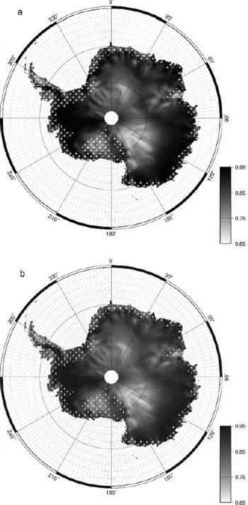
The model is optimized independently for every 50 km × 50 km pixel in Antarctica. The root of the cost-function minimum ![]() presents large variations across the continent and especially between the coastal regions and the interior (Fig. 4a). The causes of the variations are investigated hereafter.
presents large variations across the continent and especially between the coastal regions and the interior (Fig. 4a). The causes of the variations are investigated hereafter.
(a) Root-mean-square error after parameter optimization and melt zones (white crosses). (b) Root-mean-square error versus wind speed at 35 km resolution predicted by the global climate model LMDZ. The dashed line illustrates the wind-speed constraint on the rmse lower bound.

The highest rmse are found near the coasts and closely match the melt zones (white crosses in Fig. 4a). Melt zones are defined here as ‘zones where melt occurred on at least 20 days in the period 1979–2006’. They cover 17% of the continent. Daily surface melting was derived by Reference Picard and FilyPicard and Fily (2006). The error is large, despite brightness temperature observations being masked out during melt events (section 2.5). A possible explanation is that the snowpack emissivity is not constant, even when only the dry periods are considered. Indeed, some studies have shown that the emissivity occasionally drops after melt events and the relaxation to recover a ‘normal’ emissivity lasts a few years (see time series of Reference Abdalati and SteffenAbdalati and Steffen (1998); Reference Bingham and DrinkwaterBingham and Drinkwater (2000)). The emissivity drop is caused by the formation of ice layers during the refreezing of meltwater. Then, the emissivity increases slowly as new snow accumulates over the ice layers. Our model is unable to track such changes because the emissivity is assumed constant (section 2.3) and the process of ice-layer formation is not represented. Our model is therefore inadequate for the melt zones, even during the periods the snowpack is dry.
In the dry zones of the continent, the rmse ranges between 1.4 and ∼3 K. The error distribution between the channels is similar to that at Dome C (above). While larger than SSM/I noise, such error values are remarkably low, given the spatial and temporal coverage of the study. This also confirms that the low error of 2 K obtained at Byrd Station by Reference Winebrenner, Steig and SchneiderWinebrenner and others (2004) can be obtained over most of the inner Antarctic. This result inherently indicates that the temporal variations of the ERA-40 meteorological surface variables are representative of the actual conditions.
The lowest rmse values (1.4–2 K) are located around the divide in East Antarctica. Higher values (2–3 K) are found in Marie Byrd Land (90–135° W), on the Filchner Ice Shelf (30–60° W) and in the Lambert Glacier basin (60–80° E). Southward of the East Antarctica divide, rmse values are also high (2.5–3 K).
Since the rmse varies at a finer spatial scale than the resolution of ERA-40 (∼120 km), we conclude the spatial variations of rmse come in part from the model and are related to the surface characteristics. Moreover, the highest errors often correspond to known geographical features and/or distinct glaciological characteristics, such as mountains, glaciers or streams. All these regions are characterized by strong topography or very rough surface, features incompatible with the assumption of horizontal homogeneity required by the model. The error is also large in regions of strong erosion (wind-glazed surfaces) as southward of the East Antarctic divide (Reference Fahnestock, Scambos, Shuman, Arthern, Winebrenner and KwokFahnestock and others, 2000; Reference Frezzotti, Gandolfi, La Marca and UrbiniFrezzotti and others, 2002).
On the large scale in the dry zone, a broad relationship seems to exist between rmse and wind speed, as shown in Figure 4b. The mean annual wind speed was extracted from a simulation of the global climate model, LMDZ (Laboratoire de Météorologie–Zoom (Reference Krinner, Guichard, Ox, Genthon and MagandKrinner and others, 2008)). Every dot in Figure 4b represents one pixel in the dry zone, and the gray shading shows the density of dots. It appears that, for a given wind speed, the rmse presents a clear minimum that increases with wind speed (the dashed line drawn empirically in Fig. 4b).
The physical processes that may explain the dependence on wind speed include: (1) crust layer/blue ice due to wind scour, as for instance in the Lambert Glacier basin (Reference Bintanja and van den BroekeBintanja and Van den Broeke, 1995; Reference Vaughan, Bamber, Giovinetto, Russell and CooperVaughan and others, 1999) and Dronning Maud Land (Reference Bintanja and van den BroekeBintanja and Van den Broeke, 1995), (2) surface roughness (sastrugi, as between Terra Nova Bay and Dome C (Reference Frezzotti, Gandolfi, La Marca and UrbiniFrezzotti and others, 2002)), (3) windpumping which increases the diffusivity in the upper snowpack (Reference ColbeckColbeck, 1989) and (4) spatial heterogeneity due to snowdrift and redeposition. In particular, sastrugi fields are responsible for variations of the emissivity with the sensor azimuthal view angle that result in significant variations of brightness temperature (Reference Long and DrinkwaterLong and Drinkwater, 2000) (up to 2 K rms) between the different passes within a single day. However, we estimate that the day-to-day and seasonal variations are negligible, since we work with daily averages of brightness temperature. Hence, the azimuth effect is negligible in this study.
Further observations of snow temperature and year-round structural changes of the snow surface in windy regions are needed to better understand the wind dependence of the rmse.
3.2. Estimated parameters
For each parameter, we address two questions: first, is the parameter well constrained by the observations? and, second, is the maximum likelihood (ML) parameter value (i.e. the parameter set for which the cost function is minimum) physically realistic and does it agree with other estimates from the literature? The conclusions differ greatly between the parameters. The discussion and the values presented in the following are limited to the dry zone.
Emissivity
The emissivity is well constrained by the microwave observations, as shown at Dome C by the marginal likelihood function (Fig. 5), i.e. the likelihood function integrated over all the parameters except the emissivity. The marginal likelihood is peaked, symmetric and Gaussian-like. It is also much narrower than the typical emissivity distribution observed in Antarctica (ML emissivity distribution shown in gray). The ensemble mean emissivity is 0.843 (at Dome C, at the 19V channel) and closely matches the maximum likelihood emissivity of 0.844. The standard deviation is 0.027.
Emissivity marginal likelihood at Dome C (black) and distribution of the maximum likelihood emissivities over Antarctica (gray).

These results indicate that our approach is reliable for estimating emissivities, despite many parameters being free. However, it is much more resource-demanding and less practical than other widely used methods, such as the ratio between brightness temperature and annual mean air temperature (Reference Sherjal and FilySherjal and Fily, 1994) or mean surface temperature (Reference Schneider, Steig and ComisoSchneider and others, 2004). We question here whether these approaches give results equivalent to ours.
Neglecting the atmosphere, the emissivity can be estimated (Reference Sherjal and FilySherjal and Fily, 1994) by:
where 〈·〉 denotes the temporal average for 1992–2002. A better estimate is obtained by accounting for the atmosphere. Taking the average of Equation (11), the emissivity can be and estimated (see also Reference Karbou and PrigentKarbou and Prigent, 2005) by:
By applying these equations on every pixel in the dry zones using air temperature from ERA-40, we find that accounting for the atmosphere results in slightly lower snow emissivities, on average, over Antarctica: ![]() at the 19V channel, −0.014 at the 19H channel, −0.018 at the 37V channel and −0.03 at the 37H channel. In contrast, the difference, ∊
ML − ∊
annual air+atmo (where ∊
ML is the ML emissivity), is about an order of magnitude lower than the previous difference. We conclude that the ML estimates and annual method give equivalent results as long as the atmosphere is taken into account. The method based on Equation (20), being much faster than our approach, it is preferable for estimating the emissivity.
at the 19V channel, −0.014 at the 19H channel, −0.018 at the 37V channel and −0.03 at the 37H channel. In contrast, the difference, ∊
ML − ∊
annual air+atmo (where ∊
ML is the ML emissivity), is about an order of magnitude lower than the previous difference. We conclude that the ML estimates and annual method give equivalent results as long as the atmosphere is taken into account. The method based on Equation (20), being much faster than our approach, it is preferable for estimating the emissivity.
The emissivities at the four channels are significantly correlated with each other: the correlation coefficient between the 19V channel and the 37V, 19H and 37H channels is 0.96, 0.93 and 0.93, respectively. The emissivity map at the 19V channel is shown in Figure 6a. (The map at the 37V channel is given by Reference Schneider, Steig and ComisoSchneider and others (2004, fig. 2).)
(a) Emissivity and (b) apparent penetration depth at 19V channel. Penetration depth is relative to the arbitrarily chosen thermal diffusivity (5×10⁻⁷ m2 s−1 here). Melt zones are shown with white crosses.
The range of emissivity is large and several areas can be clearly distinguished on the map:
Regions with high accumulation near the coasts (except in the melting zones) have emissivities close to unity, for instance in Marie Byrd Land (0.95–0.98 at the 19V channel) and Wilkes Land near the coast (0.94).
The emissivity gradually decreases in East Antarctica between the coast and the divide where intermediate emissivities (0.80–0.90) are observed.
In the Lambert Glacier basin, in the east of the Ross Ice Shelf and in the east of the Filchner Ice Shelf, small patches have low emissivities (0.72–0.76).
The glazed and megadune regions (Reference Fahnestock, Scambos, Shuman, Arthern, Winebrenner and KwokFahnestock and others, 2000; Reference Frezzotti, Gandolfi, La Marca and UrbiniFrezzotti and others, 2002) present the lowest emissivities (0.68–0.72).
Snow grain size is certainly the main factor influencing the emissivity variations (Reference SurdykSurdyk, 2002). The emissivity is high in regions of high accumulation near the Wilkes coast or in Marie Byrd Land, where new fresh snow with fine grains falls often and metamorphism is moderated. The emissivity is low on the plateau, where snow grains are large because metamorphism operates for a long time due to low accumulation (Reference Li and ZwallyLi and Zwally, 2004). The lowest emissivities are observed where wind erosion and/or sublimation are important, such as in the glazed regions where large grains were reported (Reference Courville, Albert, Fahnestock, Cathles and ShumanCourville and others, 2007) or in the Lambert Glacier basin (e.g. sublimation map of Reference Krinner, Magand, Simmonds, Genthon and DufresneKrinner and others, 2007).
Relating more precisely the emissivities to snowpack characteristics and explaining their regional variations require rigorous electromagnetic modeling, which is beyond the scope of the present paper.
Microwave penetration depth and thermal conductivity
Unlike emissivity, the microwave penetration depth is not well constrained by the observations. The marginal likelihood function in Dome C (black in Fig. 7) is nearly as large as the distribution of ML penetration depths across Antarctica. The standard deviation at the 19V channel at Dome C is ∼2.6 m for a mean penetration of 8.1 m. This issue comes from the interdependence in the model between the microwave penetration depth and the thermal conductivity as explained below.
Penetration depth marginal likelihood at Dome C (black) and distribution of the maximum likelihood penetration depths in Antarctica (gray).

Reference SurdykSurdyk (2002) analytically shows that the microwave penetration depth controls both the amplitude of the brightness temperature variations and the phase lag between time series of air and brightness temperatures. Since these features are readily visible in the brightness temperature time series, a strong constraint could be expected. However, the microwave penetration depth and the thermal penetration depth always appear as a ratio in Reference SurdykSurdyk’s (2002) equations and never independently. As the thermal penetration depth is related to the thermal conductivity (proportional to ![]() , any uncertainty (or absence of constraint) on the thermal conductivity propagates into uncertainty (or absence of constraint) on the microwave penetration depth.
, any uncertainty (or absence of constraint) on the thermal conductivity propagates into uncertainty (or absence of constraint) on the microwave penetration depth.
However, the situation is slightly different in our model because of the surface energy budget (absent in Reference SurdykSurdyk, 2002; Reference Winebrenner, Steig and SchneiderWinebrenner and others, 2004). The heat at the surface (e.g. due to solar radiation) is evacuated toward the atmosphere (by sensible transport, longwave radiation, etc.) and toward the snowpack at a rate governed by the snowpack thermal conductivity. Hence, the thermal conductivity indirectly controls the upward or downward evacuation of heat. Since this control is independent of the microwave penetration depth, the thermal conductivity could, in principle, be constrained alone. However, it does not work in practice, probably because the surface budget parameters (albedo and aerodynamic roughness) are not well constrained (see below).
Nevertheless, we work around this issue by setting the thermal diffusivity and, hence, deriving an apparent microwave penetration depth, ![]() (apparent because it is dependent on the real thermal diffusivity), which presents interesting patterns in Antarctica, as discussed below. The thermal diffusivity, κ, is set to 5 × 10⁻⁷ m2 s−1, a rough average between other estimates (Reference Weller and SchwerdtfegerWeller and Schwerdtfeger, 1970; Reference Ewing, Falk, Bolzan and WhillansEwing and others, 1982; Reference KikuchiKikuchi, 1982; Reference Brandt and WarrenBrandt and Warren, 1997; Reference Sturm, Holmgren, König and MorrisSturm and others, 1997) and our estimates derived from temperature profiles reported by Reference SchlatterSchlatter (1972) and M. Fahnestock and others (http://nsidc.org/data/nsidc-0283.html). This value is used for the entire continent of Antarctica although snow structure (density and grain type) is known to strongly influence the thermal diffusivity (Reference Arons and ColbeckArons and Colbeck, 1995) and to vary across Antarctica.
(apparent because it is dependent on the real thermal diffusivity), which presents interesting patterns in Antarctica, as discussed below. The thermal diffusivity, κ, is set to 5 × 10⁻⁷ m2 s−1, a rough average between other estimates (Reference Weller and SchwerdtfegerWeller and Schwerdtfeger, 1970; Reference Ewing, Falk, Bolzan and WhillansEwing and others, 1982; Reference KikuchiKikuchi, 1982; Reference Brandt and WarrenBrandt and Warren, 1997; Reference Sturm, Holmgren, König and MorrisSturm and others, 1997) and our estimates derived from temperature profiles reported by Reference SchlatterSchlatter (1972) and M. Fahnestock and others (http://nsidc.org/data/nsidc-0283.html). This value is used for the entire continent of Antarctica although snow structure (density and grain type) is known to strongly influence the thermal diffusivity (Reference Arons and ColbeckArons and Colbeck, 1995) and to vary across Antarctica.
Before analyzing ![]() spatial variations, we first compared our ML estimate of
spatial variations, we first compared our ML estimate of ![]() with those obtained by two other widely used and simpler methods. Both methods are based on Fourier analysis and adapted from the estimation of the diffusivity from vertical profiles of temperature (e.g. Reference Weller and SchwerdtfegerWeller and Schwerdtfeger, 1970; Reference Sturm, Holmgren, König and MorrisSturm and others, 1997). The first method consists of measuring the phase lag between the annual variations of air and brightness temperatures (e.g. at Dome C and Lettau (Reference Sherjal and FilySherjal and Fily, 1994)). This method appeared to be unreliable in our case at many points in Antarctica and is not further discussed here. The second method is based on the ratio between the amplitudes of brightness temperature A(T
b) and air temperature A(T
air). The penetration depth is derived following Reference SurdykSurdyk’s (2002) analytical model:
with those obtained by two other widely used and simpler methods. Both methods are based on Fourier analysis and adapted from the estimation of the diffusivity from vertical profiles of temperature (e.g. Reference Weller and SchwerdtfegerWeller and Schwerdtfeger, 1970; Reference Sturm, Holmgren, König and MorrisSturm and others, 1997). The first method consists of measuring the phase lag between the annual variations of air and brightness temperatures (e.g. at Dome C and Lettau (Reference Sherjal and FilySherjal and Fily, 1994)). This method appeared to be unreliable in our case at many points in Antarctica and is not further discussed here. The second method is based on the ratio between the amplitudes of brightness temperature A(T
b) and air temperature A(T
air). The penetration depth is derived following Reference SurdykSurdyk’s (2002) analytical model:
We use the chunk method (Reference Von Storch and Zwiersvon Storch and Zwiers, 1999) with 1 year long chunks to estimate the two spectra of air and brightness temperatures, from which the annual amplitudes are deduced.
The amplitude estimates and the ML estimates are in agreement (R 2 = 0.72 in the dry zones). However the amplitude method gives objectively wrong values at the 19V channel (e.g. negative penetration) at 86 points out of 4400. At the 37V, 19H and 37H channels, the number of negative values is even larger (320 at the 37V channel, 536 at the 19H channel and 1994 at the 37H channel). However, the correlation with the ML estimate remains significant (R 2 = 0.66 at the 37V channel, R 2 = 0.63 at the 19H channel and R 2 = 0.66 at the 37H channel).
The map of apparent penetration depth derived by the amplitude method (at the 19V channel; Fig. 6b) is less noisy than derived by the ML (map not shown), and the resolution is finer (25 cf. 50 km for reasons of computational performance). The large-scale patterns are very similar, and the relatively weak correlation is mostly explained by short-scale noise present in the ML estimates, inherent to the Monte Carlo method. We conclude that the amplitude method is reliable for the V-polarization and the fastest method. The ML estimation is much slower, slightly noisy but reliable for any polarization.
The apparent penetration depth map presents similar patterns to the emissivity map (Fig. 6a). The deepest penetrations at the 19V channel are located in Marie Byrd Land (4–7 m) and on the East Antarctic divide (4–6 m). The shallowest penetrations are found in the wind-glazed surface regions and megadunes, with values as low as 0.3 m. Intermediate values are found in Wilkes Land between the coast and the divide (2.5–5 m).
Two remarkable points can be drawn. First, the apparent penetration depths in Marie Byrd Land are about twice those in Wilkes Land, although the emissivities are of the same order. Since the emissivities are similar, the true microwave penetration depths are probably similar too. The difference between the apparent penetration depths could perhaps be explained by a larger thermal diffusivity in Wilkes Land. Wilkes Land is indeed a windy region and windpumping could significantly enhance thermal transfers (Reference ColbeckColbeck, 1989), resulting in higher diffusivity. Second, the apparent penetration depth in the wind-glazed regions and megadunes (Reference Fahnestock, Scambos, Shuman, Arthern, Winebrenner and KwokFahnestock and others, 2000) is remarkably low. In these regions, the net annual accumulation is weak, or even negative, and the strong metamorphism (Reference Albert, Shuman, Courville, Bauer, Fahnestock and ScambosAlbert and others, 2004) leads to a highly permeable snowpack composed of coarse grains (Reference Albert, Shuman, Courville, Bauer, Fahnestock and ScambosAlbert and others, 2004; Reference Courville, Albert, Fahnestock, Cathles and ShumanCourville and others, 2007). High permeability and coarse grains contribute to a short microwave penetration depth and large diffusivity, both resulting in a very short apparent penetration depth.
The apparent penetration depths at the other channels present spatial variations with penetration that are similar to those at the 19V channel. The correlation coefficient between the channels is 0.7 or higher. However, the values differ greatly; the penetration is on average 1/2, 1/3 and 1/7 that at the 19V channel for the 19H, 37V and 37H channels, respectively. The difference between the two frequencies comes from the stronger scattering at the higher frequency. The shorter penetration observed for H-polarization with respect to V-polarization is explained by the transmission of the snowpack through internal layers, which is lower for H-polarized than for V-polarized waves.
Albedo and aerodynamic roughness length
The broadband surface albedo, α, and the aerodynamic roughness length, z 0, control the surface energy budget and, especially, the net incoming flux to the snowpack. The marginal likelihood functions of these two parameters at Dome C reveal that the parameters are only slightly constrained by the observations (Fig. 8).
(a) Albedo and (b) roughness length marginal likelihood functions at Dome C.

The likelihood is small for albedo, higher than ∼0.8, probably because the net radiation absorbed by the snowpack is insufficient for high albedo to warm the snowpack in summer and no other source of heat can counterbalance this default. In contrast, any value lower than 0.8 seems equally probable. Low roughness lengths seem preferred by the model, but no clear value emerges from the optimization.
It is not surprising that microwave observations do not strongly constrain the surface scheme parameters. But this is not the only cause. The compensation between processes creates an interdependence that prevents the parameters from being constrained individually (the same issue as for the penetration depth and the thermal conductivity). To illustrate this point, several parameter estimations were performed with fixed instead of free albedo. The albedo was set to values ranging between 0.60 and 0.80, and for this test the roughness length was allowed to span a larger range than given in Table 1. The ML roughness length for each estimation is shown in Figure 9a as a function of the albedo. When the albedo is fixed, the roughness length is reasonably well constrained and a clear interdependence exists between the parameters. Our interpretation is that low albedo results in an excess of heat at the surface due to the over-absorption of shortwave radiation. The model then needs a large roughness length to enhance sensible heat flux (and latent heat flux, but that is usually an order of magnitude smaller) and to evacuate this heat. Despite this interdependence, we have chosen to estimate both parameters because, in principle, the roughness length could be constrained during the polar night when the albedo has no influence and the albedo would then be constrained during the summer.
(a) Variations of rmse as a function of the albedo (solid curve). Circles represent the maximum likelihood estimate of roughness length for each value of albedo up to 0.8. (b) Monthly mean surface fluxes predicted at Dome C by our model (solid curve) and the MAR meteorological model (dashed curve): net shortwave (SWnet), net longwave (LWnet), sensible heat (H). Latent heat is weak and not shown.

Even if the albedo is not well constrained, the rmse has a (shallow) minimum at α = 0.775 (Fig. 9a). This value is realistic. However, the corresponding roughness length is unrealistically low (<10−7 m) at Dome C (Fig. 9a) and in most of East Antarctica (results from an Antarctic-wide parameter estimation with fixed albedo of 0.775; map not shown). Low values of roughness length have been reported in previous studies for the Antarctic (e.g. 2×10⁻⁵ m estimated from eddy-flux measurements on the plateau in Dronning Maud Land; 3×10⁻⁶ m over blue ice (Reference Bintanja and van den BroekeBintanja and Van den Broeke, 1995; Reference Van As, van den Broeke, Reijmer and van de WalVan As and others, 2005)), but our estimate is one or two orders of magnitude lower. The same issue appears with a different surface scheme that better describes the atmosphere stability and instability (based on the Monin–Obukhov similarity theory, after Reference King, Anderson, Smith and MobbsKing and others, 1996; Reference Gallée, Guyomarc’h and BrunGallée and others, 2001; Reference AndreasAndreas, 2002). Despite this unrealistic value, the surface fluxes predicted by our model are realistic and agree reasonably well with those from the Modèle Atmosphérique Régional (MAR) meteorological model (Reference Gallée, Peyaud and GoodwinGallée and others, 2005) in Figure 9b.
At the Antarctic scale, the maps of estimated albedo and aerodynamic roughness length are noisy because of the weak constraint. The maps do not show clear patterns and are uninteresting. A better constraint from adequate observations is necessary.
4. Conclusion
This paper questions whether an intermediate-complexity modeling of snowpack thermal evolution and microwave emission is able to accurately predict the temporal evolution of microwave brightness temperature in Antarctica. The answer is negative in the melt zone, covering ∼17% of the continent. This result was expected, as ice layers formed by refreezing have a strong influence on the snowpack emission, and our model ignores surface melting, refreezing and snowpack stratification. In contrast, our model is able to predict brightness temperature where the snowpack never melts. In the dry zones, the difference between predicted and modeled brightness temperature time series ranges between 1.4 and 3 K rms and is of the same order as the ERA-40 air-temperature error used as an input to the model (∼2 K; Reference Bromwich and FogtBromwich and Fogt, 2004). The detailed analysis of the differences shows that rapid variations (weekly and faster) are dominated by noise in the microwave observations (0.5 K rms) and no further improvements of the model can be expected for these time periods. For slower variations, model errors and errors in the ERA-40 meteorological variables limit the prediction capabilities. With the help of time series from Dome C meteorological station, we showed that the annual to interannual variations are dominated by errors in ERA-40 rather than in the model, at least for Dome C. This result is important because it suggests that ‘surface channels’ (19 and 37 GHz) of SSM/I, or similar sensors, could be useful to improve meteorological re-analysis and analysis.
The prediction error varies spatially and seems primarily related to the surface characteristics. The best predictions are obtained on the divide of the East Antarctic plateau. The worst predictions in the dry zone are seen where the wind speed, erosion and/or sublimation are strong, for instance in the Lambert Glacier basin and in the Filchner Ice Shelf, or in wind-glazed regions. The reasons for these differences remain unclear.
Overall, the model performs remarkably well given its intermediate complexity and the wide region considered. The parameter estimation is performed independently for each pixel and significantly contributes to adapting the model to the inputs and the observations. The optimization is able to compensate for some errors in the data or some modeling oversimplifications. For instance, by estimating the emissivity, any constant bias in air temperature or observed brightness temperature can be compensated for. However, the parameter optimization is not able to compensate for all the errors and does not solely explain the model performance. For example, the prediction of the surface fluxes, absent in previous studies (Reference SurdykSurdyk, 2002; Reference Winebrenner, Steig and SchneiderWinebrenner and others, 2004), plays an important role: the error at Dome C is ∼20% worse with direct forcing of snow temperature by air temperature than with the surface scheme. The strong stable boundary layer occurring frequently during the polar winter may explain this difference. The surface scheme better describes the energy exchange than a simple forcing.
The parameter optimization does not provide realistic values for all the parameters. The optimization is indeed under-constrained by the observations, given the large number of free parameters. As an important consequence, the microwave penetration depth cannot be estimated accurately since thermal diffusivity variations are unknown in Antarctica. Future work needs to address this issue in two possible ways. The first is to add physical processes to the model, in order to reduce the number of free parameters. For instance, the emission model is simple in the present formulation. It requires the emissivity and the penetration depth to be estimated for each channel (i.e. eight free parameters in total). Predicting these quantities with a simple snowpack emission model would reduce the total number of parameters and add a physical constraint. As a positive side effect, by predicting the penetration depths, the snow thermal conductivity would be better constrained by the observations than in our current model. It is worth noting that predicting H-polarization is more challenging than V-polarization, since H-polarization is sensitive to surface density variations.
The second way is to assimilate new kinds of remote-sensing observations into the model. Thermal infrared and albedo are relevant observations to constrain the surface scheme. Furthermore thermal infrared, if accurately calibrated, provides an absolute temperature reference. Other relevant observations include altimeter data for constraining the microwave penetration depth (e.g. Reference Legrésy and RémyLegrésy and Rémy, 1998), multi-incidence angle microwave temperature from the Advanced Microwave Sounding Unit (AMSU) radiometer and active microwave.
Acknowledgements
The SSM/I data were provided by the NSIDC. The Dome C AWS data were provided by the Antarctic Meteorological Research Center, University of Wisconsin, USA. We are grateful to F. Roch for administrating the 168-processor cluster at the Observatoire des Sciences de l’Univers de Grenoble (OSUG) where the simulations were run. We had fruitful discussions with B. Legrésy (Legos, Toulouse, France) about the temporal variations of surface density. This work is supported by the French Remote Sensing program (Programme National de Télédétection Spatiale) and the NIEVE project in the LEFE (Les Enveloppes Fluids et l’Environnement)/EVE (Evolution et Variabilité du climat à l’Echelle globale) program. We also thank the reviewers who suggested the azimuthal-angle dependency and provided very detailed corrections.


