2.1. ASM formalization

Suppose the equilibrium of a DSGE model is governed by the following system of nonlinear rational expectation functions.

\begin{equation*} f\left ( X_{t},S_{t},E\left ( g\left ( X_{t+1},S_{t+1}\right ) |S_{t}\right ) \right ) =0, \end{equation*}

where both functions $f(\!\cdot \!)$ and $g(\!\cdot \!)$ are known; $X_{t}$ is the vector of endogenous variables; $S_{t}=\left ( Z_{t},{W}_{t}\right ) \in \mathcal{S}$ is the vector of state variables with ${W}_{t}$ being endogenous, i.e., $W_{t}\in X_{t-1}$ , and $Z_{t}$ being exogenous;Footnote ⁴ $\mathcal{S}$ is the original state space; $E(\!\cdot |S_{t})$ is the expectation conditional of state $S_{t}$ .

The transition equation for the exogenous state variables follows an autoregressive process:

\begin{equation*} Z_{t+1} = \rho _{z}Z_{t}+\varepsilon _{Z,t+1},\text{ where }\varepsilon _{Z,t}\sim i.i.d\text{ }N\left ( 0,\sigma _{Z}^{2}\right ). \end{equation*}

Suppose that we can write the endogenous state ${W}_{t}$ as function of $Z_{t}$ plus a normal random variable $\widetilde {W}_{t}$ :

$ {W}_{t}=h\left ( Z_{t}\right ) +\widetilde {W}_{t}, $ Footnote ⁵

where function $h(\!\cdot \!)$ is known.

We can now define and work with an auxiliary state $\widetilde {S}_{t}$ and auxiliary state space $\widetilde {\mathcal{S}}$ :

\begin{equation*} \widetilde {S}_{t}=\left ( Z_{t},\widetilde {W}_{t}\right ) \in \widetilde {\mathcal{S}}. \end{equation*}

Note that while the ergodic set for the original state variables (i.e., the original simulated state domain or state space) may be rotatedly elliptical or even non-elliptical, the ergodic set for the auxiliary state variables (i.e., the simulated auxiliary state domain or state space) is always, by construction, elliptical. More importantly, this elliptical ergodic set can be effectively approximated by a rectangular grid, making it suitable in a projection method. Consequently, the ASM method operates as a projection method, utilizing grids that are specified and updated based on auxiliary ergodic sets.

Figure 2. An example of the original ergodic set (i.e., the blue non-elliptical area in panel A), original grid (i.e., the cyan rectangular area in panel A), auxiliary ergodic set (i.e., the blue elliptical/spherical area in panel B), auxiliary grid (i.e., the magenta rectangular area in panel B), function $h(z)$ , and ASM-implied grid for original states (i.e., the magenta parallelotope area in panel A).

Figure 2 provides an example of the original ergodic set, original grid, auxiliary ergodic set, auxiliary grid, function $h(Z)$ , and ASM-implied grid for two original states: one endogenous and one exogenous. Specifically, the blue non-elliptical area in panel A represents the ergodic set for the original state variables. Without transforming the original states, the grid used in a projection method would be the cyan rectangular area in panel A. The solid red line in panel A shows an example of the function h(Z). The blue elliptical/spherical area in panel B represents the ergodic set for the auxiliary state variables. The magenta rectangular area in panel B is the numerical grid that is specified and updated based on the auxiliary ergodic set and is used in a projection method. The magenta parallelotope area in panel A illustrates the grid for the $original$ state variables that is $implied$ $by$ $the$ $ASM$ $method$ . It is evident that the ASM-implied grid aligns much more closely to the original ergodic set than the grid used in the standard projection method (e.g., the cyan rectangular area in panel A). Consequently, the ASM method is more numerically stable than the standard projection method that does not use auxiliary states, as the ASM method avoids improbable states that the model cannot solve.

2.2. An ASM algorithm

Let’s assume that the decision rule is a time invariant function of auxiliary state $\widetilde {S}$ :

\begin{equation*} X=q\left ( \widetilde {S}\right ) .\text{ } \end{equation*}

We can use the following algorithm to find $q\left ( \cdot \right )$ together with $h\left ( \cdot \right )$ .

Algorithm: Choose a numerical grid for the auxiliary state space $\widetilde {\mathcal{S}},$ then initialize functions $q^{\left ( 0\right ) }\left ( \cdot \right )$ and $h^{\left ( 0\right ) }\left ( \cdot \right )$ . In addition, discretize the distribution of shock innovation $\varepsilon _{Z}$ into a vector of $J$ integration nodes $\varepsilon _{Z}=$ $\left \{ \varepsilon _{Z,j}\right \} _{j=1}^{J}$ with weight $\omega =$ $\left \{ \omega _{j}\right \} _{j=1}^{J}$ .

For each iteration $i$ starting from $1$ , implement the following steps.

1. 1. Step 1: For each node $\widetilde {S}=\left ( Z,\widetilde {W}\right )$ of the auxiliary grid, do the following:

   1. (a) Compute

      • • $X=q^{\left ( i-1\right ) }\left ( \widetilde {S}\right )$ .

      • • $E\left ( g\left ( X_{+1},S_{+1}\right ) |S\right ) =E_{\varepsilon _{Z}}\left ( g\left ( q^{\left ( i-1\right ) }\left ( \widetilde {S}_{+1}\right ), S_{+1}\right ) \right )$ , where $E_{\varepsilon _{Z}}$ is the expectation computed based on the discretized distribution of $\varepsilon _{Z},$ $\widetilde {S}_{+1}=\left ( Z_{+1},\widetilde {W}_{+1}\right ), $ ${S}_{+1}=\left ( Z_{+1},{W}_{+1}\right )$ , and

        • − $\,\,Z_{+1}=\rho _{z}Z+\varepsilon _{Z}$ ,

        • − $\,\,\widetilde {W}_{+1}={W}_{+1}-h^{\left ( i-1\right ) }\left ( Z_{+1}\right )$ and $W_{+1}\in X.$

   2. (b) Solve $X$ from the equilibrium system $f\left ( X,S,E\left ( g\left ( X_{+1},S_{+1}\right ) |S\right ) \right ) =0,$ where $S=\left ( Z,W\right )$ and $W=h^{\left ( i-1\right ) }\left ( Z\right ) +\widetilde {W}.$

2. 2. Step 2: Update $q^{\left ( i\right ) }\left ( \cdot \right )$ using $X$ that is found in Step 1.

3. 3. Step 3: Simulate the model, calculate simulated data for $W$ , $\widetilde {W}$ , and $Z$ , then

   • • update $h^{\left ( i\right ) }\left ( \cdot \right )$ by regressing $W$ on a constant, $Z$ , and higher polynomials of $Z$ if needed.

   • • update the auxiliary grid based on simulated data for $\widetilde {W}$ .

4. 4. Step 4: Stopping rule. If $||q^{\left ( i\right ) }-q^{\left ( i-1\right ) }||+||h^{\left ( i\right ) }-h^{\left ( i-1\right ) }||$ $\lt tol$ , go to Step 5. Otherwise, increase $i:=i+1$ and go back to Step 1.

5. 5. Step 5: Exit and do simulations.

Algorithm discussion: The ASM method is basically a projection method that is implemented based on an auxiliary state grid rather than the original state grid. As discussed above, the ASM method allows us to solve the model within the high-probability area of the ergodic set for the original state variables. Therefore, it helps stabilize the numerical solution method. This method combines a projection method, stochastic simulations, and state variable transformation.

There are several key points that are worth noting. First, there are different options for selecting a numerical grid/nodes for the auxiliary state space, including evenly spaced nodes, anisotropic nodes, Chebyshev nodes, or Smolyak nodes. The choice of grid depends on researcher preferences and the specific problem at hand. Second, various basis functions can be used for the numerical functional forms of $q\left ( \cdot \right ), $ such as monomials, Chebyshev’s, or splines. In this paper, I use equally spaced nodes together with cubic spline basis functions to approximate functions $q\left ( \cdot \right )$ . For those who are interested in projection methods, more details can be found in Judd (Reference Judd1998) and Miranda and Fackler (Reference Miranda and Fackler2002).

Additionally, similar considerations apply when initializing and updating the function $h\left ( \cdot \right ).$ In my application in the next section, I use a cubic function for $h\left ( \cdot \right )$ and I initialize its coefficients to zeros. To update $h\left ( \cdot \right ), $ I simulate the model for $100,000$ periods from the deterministic steady state, then use the OLS method to update the coefficients of $h\left ( \cdot \right )$ . Readers interested in the stochastic simulation literature can refer to Judd et al. (Reference Judd, Maliar and Maliar2011) for more information.

3.1. Model

The model is a standard New Keynesian model that incorporates downward nominal price and wage rigidities as in Kim and Ruge-Murcia (Reference Kim and Ruge-Murcia2009) and Gourio and Ngo (Reference Gourio and Ngo2024).

3.1.1. Composite labor

Firms need to use composite labor to produce intermediate differentiated goods. Composite labor can be created by aggregating a variety of differentiated labor indexed by $h\in \left [ 0,1\right ]$ using a CES technology

(1) \begin{equation} N_{t}=\left ( \int _{0}^{1}N_{t}^{h}{}^{\frac {\epsilon _{w}-1}{\epsilon _{w}}}dh\right ) ^{\frac {\epsilon _{w}}{\epsilon _{w}-1}}, \end{equation}

where $\varepsilon _{w}$ determines the elasticity of substitution among differentiated types of labor. The profit maximization problem is given by

\begin{equation*} \max \text{ }W_{t}N_{t}-\int _{0}^{1}W_{t}^{h}N_{t}^{h}dh, \end{equation*}

where $W_{t}^{h}$ and $N_{t}^{h}$ are the nominal wage and quantity of differentiated labor of type $h.$

Profit maximization and the zero-profit condition give the demand for labor of type $h$

(2) \begin{equation} N_{t}^{h}=\left ( \frac {W_{t}^{h}}{W_{t}}\right ) ^{-\epsilon _{w}}N_{t}, \end{equation}

and the aggregate wage level

(3) \begin{equation} W_{t}=\left ( \int \left ( W_{t}^{h}\right ) ^{1-\epsilon _{w}}dh\right ) ^{\frac {1}{1-\epsilon _{w}}}. \end{equation}

3.1.2. Final consumption goods

To produce consumption goods, households buy and aggregate a variety of differentiated intermediate goods indexed by $i\in \left [ 0,1\right ]$ using a CES technology

\begin{equation*} Y_{t}=\left ( \int _{0}^{1}Y_{t}\left ( i\right ) ^{\frac {\epsilon -1}{\epsilon }}di\right ) ^{\frac {\epsilon }{\epsilon -1}}, \end{equation*}

where $\varepsilon$ determines the elasticity of substitution among intermediate goods. The profit maximization problem is given by

\begin{equation*} \max \text{ }P_{t}Y_{t}-\int _{0}^{1}P_{t}\left ( i\right ) Y_{t}\left ( i\right ) di, \end{equation*}

where $P_{t}\left ( i\right )$ and $Y_{t}\left ( i\right )$ are the price and quantity of intermediate good $i.$

Profit maximization and the zero-profit condition give the demand for differentiated intermediate good $i$

(4) \begin{equation} Y_{t}\left ( i\right ) =\left ( \frac {P_{t}\left ( i\right ) }{P_{t}}\right ) ^{-\epsilon }Y_{t}, \end{equation}

and the aggregate price level

(5) \begin{equation} P_{t}=\left ( \int P_{t}\left ( i\right ) ^{1-\epsilon }di\right ) ^{\frac {1}{1-\epsilon }}. \end{equation}

3.1.3. Household $h$ ’s problem

There is a unit mass of households. Each household indexed by $h\in$ $\left [ 0,1\right ]$ provides type-h labor and is competitively monopolistic in the labor market. It is costly to adjust wages. Without loss of generality, we assume that households pay wage adjustment costs which have a general form

\begin{equation*} AC_{t}^{h}=\Phi \left ( \frac {W_{t}^{h}}{W_{t-1}^{h}}\right ) W_{t}^{h}N_{t}^{h}, \end{equation*}

where $\Phi ^{\prime }\left ( \cdot \right ) \gt 0$ and $\Phi ^{\prime \prime }\left ( \cdot \right ) \gt 0.$

In this paper, we follow Kim and Ruge-Murcia (Reference Kim and Ruge-Murcia2009) and use the linex function to model wage adjustment costs. Specifically,

(6) \begin{equation} \Phi _{t}^{h}=\Phi \left ( \frac {W_{t}^{h}}{W_{t-1}^{h}}\right ) =\phi _{w}\left ( \frac {\exp \left ( -\psi _{w}\left ( \frac {W_{t}^{h}}{\overline {\Pi }W_{t-1}^{h}}-1\right ) \right ) +\psi _{w}\left ( \frac {W_{t}^{h}}{\overline {\Pi }W_{t-1}^{h}}-1\right ) -1}{\psi _{w}^{2}}\right ), \end{equation}

where $\overline {\Pi }$ is the inflation used to index nominal wage in labor contracts, $\phi _{w}$ is the level parameter and $\psi _{w}$ is the asymmetry parameter. If $\psi _{w}\gt 0,$ the wage adjustment cost is asymmetric. In particular, the cost to lower a wage compared to the indexed wage in the contract is higher than to increase it by the same amount. When $\psi _{w}$ approaches $0$ , this function becomes a symmetric quadratic function around the indexed inflation.

\begin{equation*} \Phi \left ( x\right ) =\frac {\phi _{w}}{2}\left ( \frac {x}{\overline {\Pi }}-1\right ) ^{2}. \end{equation*}

Household $h$ choose $\left \{ C_{t}^{h},N_{t}^{h},W_{t}^{h},B_{t}^{h}\right \} _{t=1}^{\infty }$ to maximize the inter-temporal utility

\begin{equation*} V_{t}^{h}= u(C_{t}^{h},N_{t}^{h})+\beta E_{t}\left ( V_{t+1}^{h}\right ) \end{equation*}

with the flow utility

\begin{equation*} u\left ( C_{t},N_{t}\right ) =\frac {C_{t}^{1-\gamma }}{1-\gamma }-\frac {\chi N_{t}^{1+\eta }}{1+\eta }, \end{equation*}

subject to the labor demand (2) and the budget constraint as described below.

The budget constraint is:

(7) \begin{align}& P_{t}C_{t}^{h}+R_{t}^{-1}B_{t}^{h} = W_{t}^{h}N_{t}^{h}\left ( 1-\Phi _{t}^{h}\right ) +B_{t-1}^{h}+D_{t}^{h}+T_{t}^{h},\text{ for }t=1,..,\infty, \end{align}

(8) \begin{align}&\qquad\qquad\qquad\qquad\qquad \text{given }W_{0}\text{ and }B_{0}. \end{align}

A symmetric solution to this optimization problem, i.e., $W_{t}^{h}=W_{t}$ and $N_{t}^{h}=N_{t},$ implies a New Keynesian Phillips curve for wages and the Euler equation (see Appendix B for the derivation):

(9) \begin{align}& 0 =\left ( 1-\varepsilon _{w}\right ) \left ( 1-\Phi \left ( \Pi _{t}^{w}\right ) \right ) N_{t}-\Phi ^{\prime }\left ( \Pi _{t}^{w}\right ) \Pi ^{w}N_{t}+\varepsilon _{w}\chi \frac {N_{t}^{\eta +1}}{w_{t}C_{t}^{-\gamma }} \notag\\ &\qquad +E_{t}\left [ M_{t,t+1}\frac {\Phi ^{\prime }\left ( \Pi _{t+1}^{w}\right ) \left ( \Pi ^{w}\right ) ^{2}}{\Pi _{t+1}}N_{t+1}\right ], \end{align}

(10) \begin{align}&\qquad\qquad\qquad\qquad E_{t}\left [ M_{t,t+1}\left ( \frac {R_{t}}{\Pi _{t+1}}\right ) \right ] =1, \end{align}

where $w_{t}=W_{t}/P_{t}$ is the real wage; $\Pi _{t}=P_{t}/P_{t-1}$ is gross inflation; $\Pi _{t}^{w}=W_{t}/W_{t-1}$ is gross wage inflation. Wage inflation and the stochastic discount factor are given by

(11) \begin{align}&\qquad \Pi _{t}^{w}=\frac {w_{t}}{w_{t-1}}\Pi _{t}, \end{align}

(12) \begin{align}& M_{t,t+1}=\beta \left ( \frac {C_{t+1}}{C_{t}}\right ) ^{-\gamma }. \end{align}

Note that when $\phi _w =0$ and $\varepsilon _{w}$ $\rightarrow$ $\infty, $ equation (9) becomes a standard marginal rate of substitution between labor and consumption

\begin{equation*} \frac {\chi N_{t}^{\eta }}{C_{t}^{-\gamma }}=w_{t}. \end{equation*}

3.1.4. Intermediate goods producer $i^{\prime }s$ problem

There is a unit mass of intermediate goods producers that are monopolistic competitors. Suppose that each intermediate good $i\in \left [ 0,1\right ]$ is produced by one producer using the technology

(13) \begin{equation} Y_{t}^{i}=Z_{t}N_{t}^{i}, \end{equation}

where $N_{t}^{i}$ is composite labor input used by firm $i$ ; and

(14) \begin{eqnarray} \ln \left ( Z_{t}\right ) &=&\rho _{Z}\ln \left ( Z_{t-1}\right ) +\varepsilon _{Z,t},\text{ } \\ \varepsilon _{Z,t} &\sim &i.i.d\text{ }N\left ( 0,\sigma _{Z}^{2}\right ) . \notag \end{eqnarray}

Following Rotemberg (Reference Rotemberg1982), we assume that each intermediate goods firm $i$ faces costs of adjusting prices in terms of final goods. The adjustment cost function is in a general form

\begin{equation*} AC^i_{t}=\Gamma \left ( \frac {P_{t}^{i}}{P_{t-1}^{i}}\right ) Y_{t}, \end{equation*}

where $\Gamma ^{\prime }\left ( \cdot \right ) \gt 0$ and $\Gamma ^{\prime \prime }\left ( \cdot \right ) \gt 0.$

We also use the linex function to model price adjustment costs. Specifically,

(15) \begin{equation} \Gamma \left ( x\right ) =\phi _{p}\left ( \frac {\exp \left ( -\psi _{p}\left ( x-\overline {\Pi }\right ) \right ) +\psi _{p}\left ( x-\overline {\Pi }\right ) -1}{\psi _{p}^{2}}\right ), \end{equation}

where $\overline {\Pi }$ is the inflation used to index prices in contracts between intermediate good producers and final good producers, and $\phi _{p},\psi _{p}$ are parameters that determines the level and the asymmetry of price adjustment costs. If $\psi _{p}\gt 0,$ the price adjustment cost is asymmetric. Particularly, the cost to lower a price compared to the indexed price is higher than to increase it by the same amount. The linex function nests the symmetric quadratic cost when $\psi _{p}$ approaches $0$ , i.e., it becomes a quadratic function around the indexed inflation:

\begin{equation*} \Gamma \left ( x\right ) =\frac {\phi _{p}}{2}\left ( \frac {x}{\overline {\Pi }}-1\right ) ^{2}, \end{equation*}

which is popularly used in the literature.

The problem of firm $i$ is given by

(16) \begin{equation} \underset {\{Y_{t+j}^{i},N_{t+j},P_{t+j}^{i}\}_{j=0}^{\infty }}{\max }E_{t}\sum _{j=0}^{\infty }\left \{ M_{t,t+j}\left [ \left ( \frac {P_{t+j}^{i}}{P_{t+j}}Y_{t+j}^{i}-w_{t}N_{t}^{i}\right ) -\Gamma \left ( \frac {P_{t+j}^{i}}{P_{t+j-1}^{i}}\right ) Y_{t+j}\right ] \right \} \end{equation}

subject to its demand (4) and production function (13).

In a symmetric equilibrium where all firms choose the same price and produce the same quantity (i.e., $P_{t}^{i}=P_{t}$ and $Y_{t}^{i}=Y_{t}$ ). The optimal pricing rule then implies the New Keynesian Phillips curve,

(17) \begin{equation} \left ( 1-\varepsilon +\varepsilon \frac {w_{t}}{Z_{t}}-\Pi _{t}\Gamma ^{\prime }\left ( \Pi _{t}\right ) \right ) Y_{t}+E_{t}\left ( M_{t,t+1}\Pi _{t+1}\Gamma ^{\prime }\left ( \Pi _{t+1}\right ) Y_{t+1}\right ) =0. \end{equation}

3.1.5. Monetary policy

The central bank conducts monetary policy by setting the interest rate using a simple Taylor rule:

(18) \begin{equation} R_{t}=R^{\ast }\left ( \frac {GDP_{t}}{GDP^{\ast }}\right ) ^{\phi _{y}}\left ( \frac {\Pi _{t}}{\Pi ^{\ast }}\right ) ^{\phi _{\pi }} \end{equation}

where $GDP_{t}\equiv C_{t}$ denotes the gross domestic product (GDP); $GDP^{\ast }$ and $\Pi ^{\ast }$ denote the target GDP and inflation, respectively; $R^{\ast }$ denotes the intercept of the Taylor rule.

3.1.6. Equilibrium systems

With the Rotemberg price setting, the aggregate output satisfies

(19) \begin{equation} Y_{t}=Z_{t}N_{t}, \end{equation}

Finally, the resource constraint is given by

(20) \begin{equation} C_{t}=\left ( 1-\Gamma \left ( \Pi _{t}\right ) \right ) Y_{t}-w_{t}N_{t}\Phi \left ( \Pi _{t}^{w}\right ) . \end{equation}

The equilibrium system for the model consists of a system of seven nonlinear difference equations (9), (10), (11), (17), (18), (19), (20) for seven variables $w_{t},$ $C_{t},$ $R_{t},$ $\Pi _{t},$ $\Pi _{t}^{w},$ $N_{t},$ and $Y_{t}.$

The system of equilibrium equations is summarized in Appendix A.

3.2. Parameter calibration

Table 1 presents the calibrated parameters. All of the parameters are taken from the New Keynesian literature, except the asymmetry parameters for the price and wage adjustment cost functions, $\psi _{p}$ and $\psi _{w}$ , which I vary from 0 to 500. In particular, the subjective discount factor $\beta$ is set to $0.99$ , the intertemporal elasticity of substitution (IES) of consumption $1/\gamma$ to $0.5$ , and the Frisch elasticity of labor supply $1/\eta$ to 1.5. The gross markup for intermediate good producers is set to $1.15$ , corresponding to the demand elasticity parameter $\varepsilon =7.66$ . The labor demand elasticity parameter, $\varepsilon _{w},$ is set to $6$ , giving the labor gross markup of $20\%$ . The labor disutility parameter $\chi$ is calibrated to achieve the steady state labor of $1/3$ .

Table 1. Model parameters

In addition, I set $\Pi ^{\ast }$ (the so-called target inflation rate) and the inflation rate to be indexed $\overline {\Pi }$ to the conventional value of $2\%$ , the weight on inflation in the Taylor rule $\phi _{\pi }=$ $1.75$ , and the weight on output gap $\phi _{y}$ = $0.065$ . The adjustment cost level for prices and wages, $\phi _{p}$ and $\phi _{w}$ , are both set to 100. The asymmetry level for the price adjustment cost function, $\psi _{p}$ , and the asymmetry level for the wage adjustment cost function, $\psi _{w}$ , are allowed to vary. Except $\psi _{p}$ and $\psi _{w}$ , all the values are standard in the literature, e.g., Woodford (Reference Woodford2003).

Finally, the persistence of the TFP shock is set at $0.97$ and the standard deviation of TFP innovations is $0.65\%$ . These values help produce the standard deviation of real GDP growth being in line with the U.S. data, which is 2.3% for the period of 1990q1–2019q4.

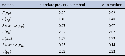
3.3. Quantitative results

I solve the fully nonlinear model using the ASM method with the algorithm described above. I also solve the model using the standard projection method, as in Judd (Reference Judd1998), Miranda and Fackler (Reference Miranda and Fackler2002), and Ngo (Reference Ngo2014). To assess the accuracy of the ASM method, I solve the benchmark model without asymmetry, i.e., $\psi _{p}=\psi _{w}=0,$ using both the ASM method and the standard projection method.Footnote ⁶ The results are presented in Table 2. As seen in this table, the key moments are nearly identical between the two methods, confirming that the ASM method is as accurate as the standard projection method when the adjustment cost functions are symmetric.Footnote ⁷ Note that the model remains fully nonlinear, so even in the absence of the asymmetry, there is still considerable nonlinearity within the model.

Table 2. Key moments from the ASM method and the standard projection method when there is no asymmetry, i.e., $ \psi _{p}= \psi _{w}=0$ . The unit is (annualized) percent

Another important result is that, for the standard projection method to produce the same results as the ASM method (as shown in Table 2), I need to substantially increase the number of nodes along the endogenous state (lagged real wage) for the standard projection method. As a result, the standard projection method converges more slowly than the ASM method.Footnote ⁸

To determine which method is able to handle higher nonlinearity, I keep the price adjustment cost asymmetry $\psi _{p}=0$ and vary the asymmetry level for the wage adjustment cost function $\psi _{w}$ from 0 to 500. I find that the standard projection method can only solve the model with $\psi _{w}$ up to $36$ , while the ASM method can solve the model with $\psi _{w}$ up to $221$ . With $\psi _{w}=220$ , the skewness of the wage inflation is about $0.48$ , which is consistent with the U.S. wage inflation data during the period 1990q1–2019q4.Footnote ⁹

Figure 3. Adjustment cost function for prices and wages.

Another way to test the ASM method’s ability to handle nonlinearity is to set the wage adjustment cost asymmetry $\psi _{w}=0$ and vary the asymmetry level for the price adjustment cost function $\psi _{p}$ from 0 to 500. The standard projection method can only solve the model with $\psi _{p}$ up to $61$ , while the ASM method can solve the model with $\psi _{p}$ up to $491$ . With $\psi _{p}=300$ , the skewness of the price inflation is about $1.19$ , which is consistent with the U.S. price inflation data during the period 1990q1–2019q4.Footnote ¹⁰ In addition, the skewness of wage inflation is $0.55$ , which is also in line with the U.S. data of $0.48$ , as discussed earlier in this paper.

It is worth noting that, for both methods, I update the grids frequently based on simulations. I also use solutions from a lower level of asymmetry as initial guesses when solving the model with a higher level of asymmetry. Moreover, I use solutions from the ASM method to compute ergodic sets for the original state variables, then use this information to specify grids and to generate initial guesses for the standard projection method.

The result confirms that the ASM method can handle the nonlinearity required to match the U.S. data, while the standard projection method cannot. The main reason for the difference is that the ergodic set of the original state variables is rotatedly non-elliptical, as shown in Figure 1 in the previous section. When using the standard projection method, we need to specify a rectangular grid that is large enough to cover this ergodic set. This leads to a significantly large set of improbable states—states that the model never visits but could cause problems for the numerical solution method. For example, the model becomes unsolvable in a state with high lagged real wage and low productivity. This state is improbable and in this state, two forces are at work, causing the $current$ nominal wage to be substantially smaller than the $previous$ nominal wage: (i) the mean reverting characteristic of real wage dynamics and (ii) lower productivity.Footnote ¹¹ The substantial decrease in nominal wage would lead to unrealistically high wage/price adjustment cost, rendering the model unsolvable in this state. However, using the ASM method, we are able to avoid most of these states. As a result, the ASM method can solve the model with much more nonlinearity.

To illustrate the nonlinearity of the model regarding $\psi _{p}$ and $\psi _{w}$ , I plot the linex function for different values of asymmetry in Figure 3. Additionally, I plot the original ergodic set, the original grid, the auxiliary ergodic set, and the auxiliary grid for the case of price asymmetry only, $\psi _{p}=300$ and $\psi _{w}=0$ , as in Figure 2. It is important to note that, based on the simulated data after solving the model using the ASM, the ergodic set for TFP and the real wage is rotatedly non-elliptical, as shown by the blue area in panel A. Ideally, we should use a numerical grid, as shown by the magenta parallelotope area in panel A, for the standard projection method. However, it is nontrivial to do such a thing. By using the ASM method, we can transform the original rotated non-elliptical ergodic set into an elliptical set that can be accurately approximated by a rectangular grid used in a projection method, as shown by the magenta rectangular area in panel B. By doing so, we can avoid most improbable original states that the model never visits but can cause problems for a numerical method.

Figure 4. Impulse response functions for the case of $ \psi _{p}=300$ . The red lines show the responses of the policy rate, real GDP, (price) inflation, wage inflation, and the real wage under a TFP shock of different magnitudes starting from the deterministic steady state. The starred blue lines present the responses under negative shocks. The unit is annualized percent.

Figure 4 displays the impulse response functions for selected macroeconomic variables in the model with asymmetric price adjustment costs only, i.e., $\psi _{p}=300$ and $\psi _{w}=0$ . The red lines represent the responses of the policy rate, real GDP, (price) inflation, wage inflation, and the real wage under a positive TFP shock of different magnitudes, starting from the deterministic steady state. The units are expressed in annualized percentages. The starred blue lines show the responses under a negative shock.

From panels A, B, C of this figure, we can see that the responses are highly dependent on the sign and the magnitude of TFP shocks. First, under a positive shock, prices decline due to lower production cost, while under a negative shock, prices increase due to higher production cost. However, because of downward nominal price rigidities, it is more costly for firms to lower prices than to raise them relative to the indexed price. As a result, the price inflation changes less under a positive shock than under a negative shock of the same magnitude. Consequently, output and the policy rate respond less under the positive shock than under the negative shock.

Second, the response of a selected variable (e.g., inflation) under a three-standard-deviation shock is more than three time greater than the one under a one-standard-deviation shock.

Therefore, based on the level of asymmetry solved by the ASM method, which generates results consistent with the skewness of the U.S. inflation distribution, the impulse responses of some selected macroeconomic variables are highly dependent on the size and the sign of fundamental shocks, indicating that the model is highly nonlinear. However, with the maximum level of asymmetry solved by the standard projection method (i.e., $\psi _{p}=61$ ), the impulse responses, shown in Figure 5, display a propagation mechanism close to those of a linear model. Specifically, responses under a positive shock are mirror images of those under a negative shock, and the magnitude of responses increases linearly with the size of the shock.

Figure 5. Impulse response functions for the case of $ \psi _{p}=61$ . The red lines show the responses of the policy rate, real GDP, (price) inflation, wage inflation, and the real wage under a TFP shock of different magnitudes starting from the deterministic steady state. The starred blue lines present the responses under negative shocks. The unit is annualized percent.

3.4. Comparing the ASM method and the principal component method

In this subsection, I will provide some numerical results to show the difference between the ASM method and the principal component (PC) method used in Judd et al. (Reference Judd, Maliar, Maliar and Valero2014) and Maliar and Maliar (Reference Maliar and Maliar2015). As I explained in the previous section, the main difference between the two methods lies in the transformation technique: while the PC method relies on a linear transformation, the ASM method uses a non-linear transformation. Additionally, the ASM method only transforms endogenous state variables into auxiliary states, while the PC method transforms all original state variables into principal components and vice versa.

Figure 6. Implied grids of the original state variables in the ASM method and the PC method.

Figure 7. Actual numerical grids in the ASM method and the PC method.

Panel A of Figure 6 illustrates the ASM-implied grid and the PC-implied grid for the original state variables of the benchmark model without asymmetry, i.e., $\psi _{p}=\psi _{w}=0$ . Specifically, the magenta rectangle shows the standard grid, i.e., a grid without any transformation. The area of black diamonds represents the PC-implied grid, while the area of red circles is the grid implied by the ASM method. We can see from this panel that the standard grid is much larger than the ergodic set, the area of solid blue circles, leading to potential numerical problems related to a grid point that the model never visits. In addition, compared to the standard grid, the grids implied by the ASM and PC methods are much smaller. They are almost the same and they cover the ergodic set neatly. It is also interesting that the implied grid points by the ASM method and the PC method are systemically different, resulting from different transformation techniques. However, the simulated results generated by the two methods are identical.

It is very important to report that the ASM is much faster than the PC method in this case. Specifically, given everything the same (including the number of grid points, the number of nodes on each state dimension, the number of simulations used to update policy function, the computing power), the time needed to solve the model using the ASM method is only 70% of the time required by the PC method. The main reason is that the ASM method only transforms endogenous state variables into auxiliary states, while the PC method transforms all original state variables into principal components and vice versa. So, the PC method is more time consuming.

Panel B of Figure 6 presents the case of asymmetry, i.e., $\psi _{p}=300$ and $\psi _{w}=0.$ The ASM-implied grid does a slightly better job than the PC method in terms of enclosing the ergodic set. In other words, the actual numerical grid used by the ASM method, shown by the rectangular area in Panel B of Figure 7, is slightly smaller than the one used by the PC method, shown by Panel A of Figure 7. As a result, the ASM method can handle a slightly larger level of asymmetry. Specifically, the ASM method can solve the model with $\psi _{p}$ up to $491$ , compared to $461$ by the PC method. Note that although the difference is relatively small in this example, it may be larger when the model has more nonlinearity, such as more asymmetry or higher risk aversion.

It is also important to note that the time needed to solve the model using the ASM method is only 63% of the time required by the PC method, even smaller than in the case of symmetry. The reason for the ASM method to be faster than the PC method in the presence of asymmetry is that the ASM method has a relatively smaller actual numerical grid that encloses the ergodic set of the auxiliary states more neatly, as seen by Figure 7. Finally, the simulated moments for macroeconomic variables are almost identical for the two methods. To save space, I do not report them here. However, they are available upon request.

Overall, the ASM method is shown to be much faster and more accurate than the PC method, at least based on the model in this paper. So, the ASM method is a valuable complement to the PC method. It provides researchers with another useful tool to deal with high nonlinearity. Which method should be used depends on researchers’ preferences and skills and the nonlinearity nature of models.