


1. Introduction
Iceberg calving is a significant source of mass loss from the Greenland and Antarctic ice sheets and many polar glaciers and ice caps (Mankoff and others, Reference Mankoff2021; Greene and others, Reference Greene, Gardner, Schlegel and Fraser2022; Reference Greene, Gardner, Wood and Cuzzone2024). By significantly altering the force balance near glacier termini, calving losses can trigger dynamic changes in the grounded interior and substantially increase ice flux into the oceans (e.g. Howat and others, Reference Howat, Joughin, Tulaczyk and Gogineni2005; Wuite and others, Reference Wuite2015; Bondzio and others, Reference Bondzio2017; Cassotto and others, Reference Cassotto2019; Miles and others, Reference Miles, Stokes, Jenkins, Jordan, Jamieson and Gudmundsson2020; Barnes and others, Reference Barnes, Gudmundsson, Goldberg and Sun2025). Despite its importance, however, calving remains poorly represented in prognostic ice-sheet models, and different calving parameterisations produce widely differing predictions of ice volume change under similar forcings (e.g. Edwards and others, Reference Edwards2019; Seroussi and others, Reference Seroussi2023; Morlighem and others, Reference Morlighem2024). Consequently, future calving losses constitute one of the largest sources of uncertainty in predictions of sea-level rise (Li and others, Reference Li, DeConto and Pollard2023).
In modelling studies of the Antarctic ice sheet, the problem of calving is often framed in terms of the hypothetical marine ice-cliff instability (MICI), in which serial collapse of tall ice cliffs is invoked as a mechanism for rapid ice retreat and collapse (e.g. Pollard and others, Reference Pollard, DeConto and Alley2015; DeConto and others, Reference DeConto2021). Comparison of simulations ‘with MICI’ and ‘without MICI’ (e.g. Li and others, Reference Li, DeConto and Pollard2023; Stokes and others, Reference Stokes, Bamber, Dutton and DeConto2025) highlights the potential impact of this mechanism, with substantially higher sea-level predictions if MICI is taken into account. The unobserved phenomenon of MICI remains controversial (e.g. Clerc and others, Reference Clerc, Minchew and Behn2019; Pattyn and Morlighem, Reference Pattyn and Morlighem2020), and some modelling studies suggest that potentially unstable ice cliffs do not necessarily lead to runaway ice-cliff collapse (e.g. Bassis and others, Reference Bassis, Berg, Crawford and Benn2021; Morlighem and others, Reference Morlighem2024). Justifiable scepticism about MICI, however, risks obscuring the fact that calving can drive rapid ice loss even in the absence of ice-cliff collapse. Recent examples include sustained episodes of rapid retreat of Jakobshavn Isbrae and Zachariæ Isstrøm in Greenland (e.g. Joughin and others, Reference Joughin2008; Mouginot and others, Reference Mouginot2015) and the collapse of Larsen B Ice Shelf in 2002 (Rack and Rott, Reference Rack and Rott2004). MICI is only one aspect of the calving problem and likely only relevant in extreme circumstances. Current prognostic ice-sheet models cannot reliably predict any calving processes, and until this major deficiency is addressed major uncertainties will persist in projecting future sea-level rise.
The problem of framing a reliable calving function for ice-sheet models does not reflect a lack of understanding of calving processes. Recent advances in both observational capability and modelling techniques have greatly increased our knowledge of calving processes and their environmental and glaciological controls (e.g. Benn and Åström, Reference Benn and Åström2018; Alley and others, Reference Alley2023; Bassis and others, Reference Bassis2024). For example, individual calving events can be simulated with great realism using the Helsinki Discrete Element Model, which models fracture from first principles and allows a range of calving styles to emerge spontaneously in appropriate settings (Åström and others, Reference Åström2013; Benn and others, Reference Benn2017, Reference Benn2023; Crawford and others, Reference Crawford2024). Furthermore, significant progress has been made in modelling interactions between fracture propagation and viscous deformation using continuum damage methods and other approaches (e.g. Jiménez and others, Reference Jiménez, Duddu and Bassis2017; Duddu and others, Reference Duddu, Jiménez and Bassis2020; Wolper and others, Reference Wolper2021; Huth and others, Reference Huth, Duddu, Smith and Sergienko2023; Rousseau and others, Reference Rousseau, Gaume, Blatny and Lüthi2024). A wide gap, however, still exists between such detailed models and the simple parameterisations required for large-scale and long-term ice-sheet simulations. In prognostic ice-sheet models, ice is represented as a continuous medium and calving losses must be simulated using some rule that specifies either the rate of ice-front retreat or the location of the ice front at any given time. The problem, therefore, is how to translate our understanding of complex calving processes into the simple functions needed for ice-sheet models.
It has become customary to refer to the functions used to prescribe calving in ice-sheet models as ‘calving laws’. Most of these functions are not laws in any physical sense, and none make reliable predictions in all but quite constrained conditions. For this reason, throughout this paper, we refer to calving functions rather than calving laws, unless in the particular context of the unknown general calving law that we seek.
An important but rarely asked question regarding calving functions is what, exactly, do we require them to do? A general answer might be, to define the position of the ice front at some arbitrary time into a simulation, but this immediately raises the issue of timescales. For simulations of entire ice sheets over multiple decades, it is neither possible nor desirable to predict individual calving events (e.g. the release of tabular bergs from ice shelves or buoyant calving events from tidewater glaciers), although that may be a valid aim for smaller-scale, shorter-term process studies. At the spatial and temporal scales relevant to ice-sheet modelling, annual mean positions may be most appropriate. Importantly, however, many ice fronts fluctuate on seasonal and multi-annual timescales, and the magnitude and duration of such fluctuations may be significant for longer-term stability (e.g. Joughin and others, Reference Joughin, Shean, Smith and Floricioiu2020). For some applications, therefore, a calving function should be capable of reproducing observed calving cycles as well as longer-term change.
To be worthy of the name, a calving law should be capable of accurately predicting calving behaviour at a broad range of geometric and dynamic settings without the need for tuning on a case-by-case basis. That is, a calving law should be equally applicable to grounded glacier termini in Alaska, seasonally floating termini in Greenland, and Antarctic ice shelves under conditions of advance, retreat and stability, using a single set of parameters. None of the calving functions currently used in ice-sheet models come close to meeting these criteria. Indeed, it may be asked if such a general calving law is even possible or mere wishful thinking.
In this paper, we argue that a general calving law is within sight and map out a strategy for finding it. To do this, we draw upon three well-established but hitherto unconnected regularities in calving system behaviour to argue that calving systems exhibit self-organisation at different scales. First, collectively, calving events have consistent statistical properties that reflect underlying fragmentation processes (Åström and others, Reference Åström2014, Reference Åström, Cook, Enderlin, Sutherland, Mazur and Glasser2021; Walter and others, Reference Walter, Lüthi and Vieli2020). Second, within the wide diversity of calving processes, two distinct styles have been identified: serac calving operating at the scale of the frontal ice cliff, and full-depth calving (including buoyant calving and tabular rifting) operating at larger scales (Medrzycka and others, Reference Medrzycka, Benn, Box, Copland and Balog2016; Fried and others, Reference Fried2018; Bézu and Bartholomaus, Reference Bézu and Bartholomaus2024; Goliber and Catania, Reference Goliber and Catania2024). Third, calving glaciers and ice shelves commonly exhibit persistent spatio-temporal patterns of advance and retreat, including seasonal and longer-term fluctuations around lateral or basal pinning points interspersed with periods of instability and transition (e.g. Murray and others, Reference Murray2015a; Bevan and others, Reference Bevan, Luckman, Benn, Cowton and Todd2019; Joughin and others, Reference Joughin, Shean, Smith and Floricioiu2020; Bassis and others, Reference Bassis2024). We argue that these regularities are intimately connected, and that calving is inherently a stochastic process that gives rise to the observed range of emergent behaviour.
Stochastic dynamic systems can be described in terms of their attractors, which can take the form of fixed points, in which the system converges on a single stable or critical state, or limit cycles, in which the system fluctuates around or within a subset of states. Serac calving bears close similarities to classical self-organising criticality, while at the larger system scale, calving fronts have a tendency to cycle around quasi-stable states governed by topography, environmental forcing and ice dynamics. The statistical properties of calving events thus provide a vital link between detailed calving processes and spatio-temporal patterns of ice-front behaviour. In turn, this opens up the possibility that a general calving law can be found by leveraging the stochastic nature of calving events and the self-organising tendencies of calving glacier systems.
In the first part of this paper, we review the statistical properties of calving events and their relationship with calving processes and patterns of ice-front fluctuations and discuss how these can be regarded as self-organising phenomena. We then review the strengths and weaknesses of commonly used calving functions and consider the degree to which they allow key behaviours to emerge in ice-sheet models. We then develop a stochastic calving function and illustrate its capabilities in simulations with Elmer/Ice for two synthetic glacier geometries representative of a Greenland outlet glacier and an Antarctic ice shelf. Finally, we discuss the implications of this work for the search for a general calving law for ice-sheet models. Throughout the paper, we focus on observed calving processes and do not consider ice-cliff collapse or MICI. The challenges involved in understanding and modelling these processes will be addressed in a separate work.
2. Statistical properties of fragmentation and calving events
Åström and others (Reference Åström, Cook, Enderlin, Sutherland, Mazur and Glasser2021) have argued that populations of calved icebergs can be described by generic fragment size distributions with two distinct components (Fig. 1). These can be expressed as:
 \begin{equation}n\left( S \right) = {c_1}{S^{ - \alpha }}{\text{exp}}\left( { - S/{S_{01}}} \right) + {c_2}{\text{exp}}\left( { - S/{S_{02}}} \right)\end{equation}
Theoretical and observed fragment and calving-size distributions. (a) Power-law and exponential iceberg size distributions, showing number of fragments (n) by size (S) on a log–log plot; (b) Observed calving volume distributions from small Svalbard glaciers (Tunabreen, Kronebreen, Sveabreen), large Greenland glaciers (Helheim, Kangerlussuaq) and Antarctic ice shelves (data compiled by Åström and others, Reference Åström2014, sources cited therein).

where  $\alpha $ takes values that arise from universal fracture processes in elastic-brittle materials, n is the number of fragments of size interval S, c 1 and c 2 are constants and S 01 and S 02 are characteristic size intervals of a specific fragmentation process.
The first term on the right-hand side of Eqn (1) is a power-law distribution with an exponential cutoff at larger fragment sizes due to the finite size of the system. Power-law distributions are characteristic of correlated fragmentation events governed by scale-invariant patterns of fracture branching and coalescence (Kekäläinen and others, Reference Kekäläinen, Åström and Timonen2007; Åström, Reference Åström2006). The second term describes an exponential distribution, which is the outcome of independent and uncorrelated fracture events with a constant probability of occurrence; large events are less common than smaller ones due to the accumulated probability that calving has already occurred.
In some cases, calving event- and iceberg size distributions have log-normal distributions (Wadhams, Reference Wadhams1988; Åström and others, Reference Åström2014; Walter and others, Reference Walter, Lüthi and Vieli2020). This distribution is expressed as:
 \begin{equation}n(S) = \frac{{{c_3}}}{S}\exp [ - {(In(S) - \phi )^2}/2{\sigma ^2}]\end{equation}
where  ${c_3}$ sets the scale for n, $\sigma $ sets the variance and $\phi $ determines the position of the maximum of the distribution. Like the exponential distribution, the log-normal distribution reflects independent and uncorrelated fracture events, but with probabilities of iceberg sizes clustered in a particular size range.
The presence of power-law, exponential and log-normal distributions in calving-size data indicates that calving from tidewater glaciers and ice shelves can be usefully considered at two scales. Power-law distributions are characteristic of relatively small-scale calving, which we term the ice-cliff scale, while the exponential and log-normal distributions describe larger, full-depth calving events along rifts or fractures located tens to hundreds of metres behind the calving front, which we term the ice-tongue scale. This subdivision is consistent with field studies that have identified end-member calving styles on Greenland tidewater glaciers, sometimes termed serac calving, buoyant calving and tabular calving (e.g. Medrzycka and others, Reference Medrzycka, Benn, Box, Copland and Balog2016; Fried and others, Reference Fried2018; Bézu and Bartholomaus, Reference Bézu and Bartholomaus2024; Goliber and Catania, Reference Goliber and Catania2024), and the distinction between calving at ice fronts and large-scale tabular calving events on ice shelves (Fricker and others, Reference Fricker, Young, Allison and Coleman2002; Sartore and others, Reference Sartore, Wagner, Siegfried, Pujara and Zoet2025).
For serac calving at the ice-cliff scale, cracks form a multitude of branches that readily merge to form additional fragments (Åström and others, Reference Åström, Cook, Enderlin, Sutherland, Mazur and Glasser2021). Such events typically involve detachment of part of the frontal ice cliff (e.g. How and others, Reference How2019; Vallot and others, Reference Vallot2019) but can include full-thickness events extending up to ∼100 m from the glacier margin (Bézu and Bartholomaus, Reference Bézu and Bartholomaus2024). In contrast, for buoyant and tabular calving at the ice-tongue scale, initial cracks develop far from each other and propagate more slowly and independently. For the exponential distribution, cracks can be assumed to develop at random locations with equal probability, whereas log-normal distributions indicate higher fracture probabilities at particular locations due to local factors favouring calving.
On individual glaciers, calving may occur at both the ice-cliff and ice-tongue scales, or only at the ice-cliff scale. For small, well-grounded tidewater glaciers, large, full-thickness calving events may be rare or absent because their ice tongues are usually not subject to sufficiently high stresses. In such cases, the entire population of calving events can be described by a power-law, such as in Svalbard where portions of subaerial ice cliffs are observed to fail in frequent, small-scale calving events (e.g. Åström and others, Reference Åström2014; Chapuis and Tetzlaff, Reference Chapuis and Tetzlaff2014; Vallot and others, Reference Vallot2019). In contrast, larger tidewater glaciers and ice shelves can exhibit power-law, exponential and log-normal calving-size distributions, representing calving at both the ice-cliff and ice-tongue scales (Åström and others, Reference Åström2014).
3. Self-organisation and ice-front fluctuations
3.1. Calving at the ice-cliff scale
Power-law distributions are characteristic of many natural systems, including those that exhibit self-organised criticality. Self-organising critical systems have a critical point as an attractor; that is, the system converges on the threshold between stable (sub-critical) and unstable (super-critical) states. The classic example is a sandpile to which grains are added slowly from above (Bak and others, Reference Bak, Tang and Wiesenfeld1987). As grains accumulate, the pile steepens until a critical slope angle is reached, whereupon a single extra grain can potentially trigger an avalanche of a random size to transfer grains downslope, maintaining the slope angle close to the critical value if the avalanche is small or returning the sandpile to a sub-critical state if the avalanche is large. If no avalanches occur, continuing addition of grains leaves the sandpile in a metastable super-critical state. In response to the opposing processes of grain accumulation and avalanching, the sandpile system spontaneously evolves towards the critical slope between sub-critical and super-critical regimes (Bak and Paczuski, Reference Bak and Paczuski1995).
In the case of calving glaciers, the critical state finds expression in the almost universal tendency for calving fronts to form near-vertical cliffs. Any perturbations that tend to over-steepen the subaerial ice cliff (e.g. forward bending due to ice deformation or undercutting by submarine melting) result in an increase in tensile and shear stresses, leading to failure events (Slater and others, Reference Slater, Benn, Cowton, Bassis and Todd2021). Subaerial ice cliffs consequently remain perched close to the point of failure on the threshold between sub-critical and super-critical states (Åström and others, Reference Åström2014; Chapuis and Tetzlaff, Reference Chapuis and Tetzlaff2014; Vallot and others, Reference Vallot2019; Walter and others, Reference Walter, Lüthi and Vieli2020). Submerged ice fronts may also be subject to overcutting, in which calving above or close to the waterline leads to the development of a projecting ice foot (Abib and others, Reference Abib2023). Such projections grow in length until they calve in response to buoyant forces, in a much longer cycle around a critical state than is typical for subaerial cliffs.
From dimensional arguments, the exponent  $\alpha $ in Eqn (1) is equal to 1.67 for fragment size distributions (Kekäläinen and others, Reference Kekäläinen, Åström and Timonen2007). However, field observations are recorded in terms of calving events, which commonly consist of multiple smaller fragments. For ice-cliff calving-size distributions, $\alpha $ is typically ∼1.2. This value is similar to that for avalanche-size distributions in some Abelian sand pile models (Priezzhev and others, Reference Priezzhev, Ktitarev and Ivashkevich1996), although the physical reason for this value remains obscure. Higher values of $\alpha $ are found in populations of calved icebergs that have undergone grinding and crushing within ice mélange, during which larger icebergs are continuously broken into smaller pieces (Åström and others, Reference Åström, Cook, Enderlin, Sutherland, Mazur and Glasser2021). Values of around 1.5 appear when the fragmentation process is essentially two-dimensional (2-D).
Ice cliffs change position through time as a result of the competing processes of ice flow, which advects the cliff forward, and calving losses, which cause it to retreat. For many tidewater glaciers, the primary driver of ice-cliff calving is submarine melting, which undercuts the ice front and triggers episodic calving of the subaerial cliff (e.g. Bartholomaus and others, Reference Bartholomaus, Larsen and OʼNeel2013; Truffer and Motyka, Reference Truffer and Motyka2016; Fried and others, Reference Fried2018; Holmes and others, Reference Holmes, Kirchner, Kuttenkeuler, Krützfeldt and Noormets2019; How and others, Reference How2019). Submarine melting is typically at a maximum in late summer when ocean or fjord waters are warmest and plume-driven circulation is most vigorous, and at a minimum during winter and spring, imparting a strong seasonal cycle on calving rates (Luckman and others, Reference Luckman, Benn, Cottier, Bevan, Nilsen and Inall2015). Where ice velocities are relatively low, submarine melt and calving rates may outpace ice velocity during the summer months leading to frontal retreat, whereas low melt- and calving rates during winter may permit ice advance. These relationships are clearly shown in Fig. 2, which presents data from Kronebreen, Svalbard. The annual velocity cycle of the glacier consists of an early summer speed-up, followed by a mid-summer slowdown, and a gradual increase to steady velocities in winter (Fig. 2a, b; How and others, Reference How2017). Frontal ablation rate (calving plus subaqueous melt of the front) has a strong positive correlation with subsurface fjord temperature (Fig. 2c, d; Luckman and others, Reference Luckman, Benn, Cottier, Bevan, Nilsen and Inall2015; Holmes and others, Reference Holmes, Kirchner, Kuttenkeuler, Krützfeldt and Noormets2019). In combination, these out-of-phase velocity and frontal ablation fluctuations result in an annual advance-retreat cycle, with advance in the first half of the year and retreat in the second (Fig. 2c). Calved icebergs are typically small and melt rapidly, ice mélange does not form in winter, and sea ice appears to play no significant role in suppressing calving. In summer, local patterns of ice retreat are strongly influenced by the position and activity of plumes fed from subglacial conduits (How and others, Reference How2017). Throughout the record shown in Fig. 2, annual frontal ablation outpaced forward advection of the front, resulting in an overall retreat of ∼2 km.
Time series of (a) near-terminus ice speed, (b) air temperature (orange) and precipitation (dark blue), (c) ice-front position (blue) and frontal ablation rate (pink) at Kronebreen, Svalbard. (d) Relationship between fjord water temperature at 20–60 m depth and frontal ablation rate from Luckman and others (Reference Luckman, Benn, Cottier, Bevan, Nilsen and Inall2015).

On fast-flowing tidewater glaciers in Greenland, ice velocities may exceed submarine melt rates at all times of year (e.g. Xu and others, Reference Xu, Rignot, Fenty, Menemenlis and Flexas2013; Kajanto and others, Reference Kajanto, Straneo and Nisancioglu2023). On such glaciers, ice cliffs will be more or less continuously advected forward and ice-front fluctuations will be determined by processes acting at the ice-tongue calving scale (Section 3.2). (Note that submarine melting can influence calving on fast tidewater glaciers through its impact on iceberg mélange or the stability of floating ice tongues, but this affects the frequency of full-depth calving events, not ice-cliff calving). Thus, depending on the relative importance of ocean forcing and ice dynamics, ice-cliff calving may or may not be the rate-controlling process on ice-front evolution.
In summary, calving at the ice-cliff scale (or serac calving) exhibits characteristics indicative of self-organising criticality (Vallot and others, Reference Vallot2019; Walter and others, Reference Walter, Lüthi and Vieli2020; Åström and others, Reference Åström, Cook, Enderlin, Sutherland, Mazur and Glasser2021). The calving rate is paced by processes that perturb the system by oversteepening the subaerial ice cliff, the most important of which is melt-undercutting. The ice-front position at any point in time is determined by the relative magnitudes of the calving rate and ice flow velocity. Changes in ice-front position, in combination with external forcings, may drive the system into deeper water with possible consequences for calving at the ice-tongue scale.
3.2. Calving at the ice-tongue scale
At the ice-tongue scale, calving includes tabular rifting and large-scale buoyant flexure (e.g. Joughin and MacAyeal, Reference Joughin and MacAyeal2005; Amundson and others, Reference Amundson, Truffer, Lüthi, Fahnestock, West and Motyka2008; James and others, Reference James, Murray, Selmes, Scharrer and O’Leary2014; Wagner and others, Reference Wagner, James, Murray and Vella2016; Benn and others, Reference Benn2017; Alley and others, Reference Alley2023). These calving styles are often classed as two distinct processes, although they are probably better regarded as end members of a continuum in which calving can occur in response to different combinations of tensile and buoyant forces. Full-depth calving events are typically preceded by the formation and propagation of fractures, which may take the form of basal crevasses or full-depth rifts, on timescales ranging from hours to years (e.g. Fricker and others, Reference Fricker, Young, Allison and Coleman2002; Bassis and others, Reference Bassis, Fricker, Coleman and Minster2008; Murray and others, Reference Murray2015a; Alley and others, Reference Alley2023).
Where buoyant or tabular calving are the dominant styles (e.g. on buoyant or near-buoyant tidewater glaciers and ice shelves) ice fronts typically exhibit asymmetric saw-tooth patterns of advance and retreat on sub-seasonal to multi-annual timescales (Fricker and others, Reference Fricker, Young, Allison and Coleman2002; Fried and others, Reference Fried2018; Bézu and Bartholomaus, Reference Bézu and Bartholomaus2024).
Ice-front positions can fluctuate around similar positions for many years, typically at narrow or shallow points within a fjord or at the mouths of embayments, collectively known as pinning points. For example, the terminus position of Store Glacier,Footnote 1 West Greenland, has remained close to the same pinning point for over 70 years (Weidick, Reference Weidick, Williams and Ferrigno1995; Benn and others, Reference Benn2023; Fig. 3), while other glaciers in Greenland (e.g. Helheim, Kangerlussuaq and Jakobshavn Isbrae) exhibit periods of relative stability interspersed with retreat (and occasionally advance) to new quasi-stable positions (e.g. Murray and others, Reference Murray2015b; Bevan and others, Reference Bevan, Luckman, Benn, Cowton and Todd2019; Joughin and others, Reference Joughin, Shean, Smith and Floricioiu2020; Fig. 4).
Ice-front fluctuations of the north, central and south sectors of Store Glacier (from Benn and others, Reference Benn2023).

Ice-front position and velocities of Helheim Glacier. The horizontal red bars show three periods where the glacier had similar minimum ice-front positions for multiple successive years, and the green arrows indicate periods of transition.

Antarctic ice shelves also commonly exhibit advance-retreat cycles, but on longer timescales than in Greenland. Front positions of Amery Ice Shelf are shown in Fig. 5 (Fricker and others, Reference Fricker, Young, Allison and Coleman2002; Bassis and others, Reference Bassis2024). The ice shelf flows out of an embayment, beyond which it is unconfined. The ice front was located several tens of km beyond the embayment in the 1950s and early 1960s, and then between 1963 and 1965 calved back to a position close to the embayment mouth. The ice readvanced between 1965 and 2018, reaching a position close to that of 1963 before calving along rifts resulted in partial loss of the shelf. Although only one sequence of retreat and advance is represented in these data, they suggest a calving cycle length of 50–60 years.
Ice-front positions of Amery Ice Shelf, East Antarctica, from 1936 to 2022 showing cycle of advance and retreat. From Bassis and others (Reference Bassis2024) after Fricker and others (Reference Fricker, Young, Allison and Coleman2002).

Shorter calving cycles for Pine Island Ice Shelf are shown in Fig. 6. Prior to 2015, the shelf exhibited calving cycles of 5–6 year duration, with advances beyond, and calving back to, a position close to lateral pinning points. Since that time, calving cycle length decreased, ice velocity increased and overall retreat occurred. These changes were initiated by progressive loss of contact with the pinning point on the eastern side of the shelf (Arndt and others, Reference Arndt, Larter, Friedl, Gohl and Höppner2018; Miele and others, Reference Miele, Bartholomaus and Enderlin2023). The front of Pine Island Glacier is currently advancing as an unconfined ice shelf, but further large calving events may be expected in the near future.
Calving cycles on Pine Island Ice Shelf. Note decrease in calving cycle length since 2014 and ice-flow acceleration after 2017.

The exponential and log-normal calving-size distributions for calving events at the ice-tongue scale indicate that advance-retreat cycles of tidewater glaciers and ice shelves can be understood in terms of calving probabilities. When ice advances beyond a pinning point, support from the glacier bed and sides is reduced or lost, so the driving stresses must be largely or entirely supported by membrane stresses from upstream. The resulting increased tensile or rotational stresses on the ice tongue will lead to increased probabilities of fracture propagation and calving (Benn and others, Reference Benn2023). For fast-flowing tidewater glaciers in Greenland, such as Store Glacier, calving probabilities are high and waiting times between calving events are short, resulting in sub-seasonal calving cycles (Fig. 3). In contrast, on ice shelves such as Pine Island Glacier prior to 2014, calving probabilities are low and waiting times between events are on the order of years to decades. Where calving probabilities are very low, unconfined ice tongues can advance far beyond pinning points before calving occurs, such as Drygalski Glacier Tongue (Indrigo and others, Reference Indrigo, Dow, Greenbaum and Morlighem2021), Amery Ice Shelf (Fricker and others, Reference Fricker, Young, Allison and Coleman2002) and Thwaites Glacier ice tongue prior to 2010 (MacGregor and others, Reference MacGregor, Catania, Markowski and Andrews2012).
Calving probabilities vary in space and time. Spatially, fracture propagation events can be expected to cluster where tensile or buoyant stresses are highest, such as near grounding lines or pinning points (e.g. Arndt and others, Reference Arndt, Larter, Friedl, Gohl and Höppner2018; Alley and others, Reference Alley2021; Benn and others, Reference Benn2022, Reference Benn2023; Bassis and others, Reference Bassis2024). Temporally, variations in calving probabilities can be imposed on seasonal timescales by the formation and breakup of rigid ice mélange. Mélange provides backstress on glacier termini, reducing calving probabilities and allowing the ice to advance in late winter and spring, but when the mélange breaks up the probability of calving increases and ice retreats (e.g. Joughin and others, Reference Joughin, Shean, Smith and Floricioiu2020; Bevan and others, Reference Bevan, Luckman, Benn, Cowton and Todd2019). During winters when persistent mélange fails to form, advance may be prevented potentially initiating longer-term retreat. On longer timescales, calving probabilities can increase in response to the weakening or loss of pinning points, such as can be seen in the decrease of calving cycle length on Pine Island Ice Shelf (Fig. 6), and more dramatically in the demise of Larsen A and B in 1998 and 2002, respectively (Doake and others, Reference Doake, Corr, Rott, Skvarca and Young1998; Scambos and others, Reference Scambos, Hulbe, Fahnestock and Bohlander2000).
In Section 3.1, we showed that frontal ice cliffs can be regarded as self-organising critical systems. Is the same true at the larger system scale relevant to buoyant and tabular calving? Cook and others (Reference Cook, Christoffersen, Truffer, Chudley and Abellan2021aReference Cook, Christoffersen and Todd, b) and Benn and others (Reference Benn2023) have argued that calving cycles at Store Glacier are indicative of self-organising criticality, in which the front continually fluctuates around a critical point determined by environmental boundary conditions. This, however, is not strictly correct. Although the pinning point at Store Glacier can be regarded as an attractor, it is not a critical point. At Store Glacier and many other glaciers, ice can advance for some distance beyond pinning points before calving occurs. In Greenland, waiting times between calving events are typically short (days, weeks, months), while for Antarctic ice shelves waiting times are long (years, decades), reflecting contrasting probabilities of calving occurring within any particular time interval.
Ice tongues, therefore, exhibit key characteristics of self-organising systems, but with attractors that are not critical points. Rather, the trajectories through time and space defined by ice-front fluctuations can be regarded as limit cycles tied to pinning points, which are stable within certain ranges of environmental conditions. If ice advances beyond a pinning point, increased stresses on the ice will increase the probability of calving and the front will retreat back towards the pinning point. Conversely, if the ice retreats behind the pinning point, lateral or basal drag provide more support for the ice front, calving probabilities decrease and the ice can advance. Perturbations to the system, such as increased surface ablation or submarine melt, or a decrease in winter mélange may or may not be large enough to push the system out of one stable position and initiate a period of transition towards another.
Figure 7 shows the co-variance of frontal positions and ice velocities of Helheim Glacier for three periods when the glacier had similar minimum positions for several years in a row (1988–2003, 2008–14 and 2017–23) using the data presented in Fig. 4. This diagram is not intended as a formal phase portrait of a 2-D dynamic system but serves to illustrate the concept of attractors in a tidewater glacier context. During each period, ice-front positions and velocities followed trajectories within small, mostly non-overlapping regions of the diagram, and between periods the glacier rapidly transitioned from one region to another (data from transitional periods not shown for clarity). The three regions represent distinct states that the glacier adopted under changing environmental conditions. Transitions between states take the form of rapid jumps, consistent with threshold behaviour.
Ice-front positions and velocities for Helheim Glacier for the periods 1988–2000, 2008–12 and 2017–23, illustrating three quasi-stable states of the system.

4. Do existing calving functions predict emergent self-organising behaviour?
4.1. Overview
In contrast with the rich variety of behaviours exhibited by calving glaciers and ice shelves, prognostic ice-sheet modelling studies commonly adopt very simple rules to prescribe what happens at calving margins. These include (1) fixed marine margins where the ‘calving rate’ is assumed equal and opposite to the ice velocity; (2) a minimum thickness condition for ice shelves; (3) ice is allowed to retreat but not advance; and (4) a prescribed calving rate (e.g. Seroussi and others, Reference Seroussi2023, Reference Seroussi2024). Such rules can be useful if the primary aim is to evaluate the impact of other model choices in a set of simulations, but they are essentially prescriptive and cannot predict how ice fronts will evolve in different circumstances. Here, we focus on predictive calving functions whose performance can be tested against observations.
Calving functions are used to frame predictions in two ways, to define either (1) the rate at which ice is removed from the front (rate functions) or (2) the location where calving occurs (position functions). Rate functions treat calving as a velocity or rate at which the ice front retreats. This is consistent with the quasi-continuous nature of ice-cliff calving but for buoyant and tabular calving, rate functions rely on the implicit assumption that multiple events integrated over some timescale can be usefully expressed as a rate. However, because buoyant and tabular calving events are commonly focused at specific geographical locations (e.g. grounding lines or down-flow of pinning points), time-averaged calving ‘rates’ simply reflect the rate of delivery of the ice to that position (van der Veen, Reference van der Veen1996; Benn and others, Reference Benn2023; Crawford and others, Reference Crawford2024). In such cases, calving position is the key variable, and position functions are more consistent with how calving operates.
The performance of a calving function depends critically upon the model environment in which it is embedded. Three aspects of model structure are particularly important. First, calving predictions based on stress metrics are obviously dependent on the way the stresses are computed. Models that solve the full Stokes equations compute all stress components including vertical shear and bending stresses and, in principle, contain enough information to predict a wide range of calving processes. Such models, however, are computationally demanding and prognostic ice-sheet models typically use reduced stress schemes. Vertically-integrated models, for example, neglect vertical shear and bending stresses and compute averaged horizontal extensional and compressional stresses through the whole ice column. Thus, although considerably faster than full-stress models, vertically integrated models have less information content with which to make a calving prediction.
Second, the type of model grid has important implications for the implementation of calving predictions. Prognostic ice-sheet models generally use fixed grids (sometimes with adaptive resolution), in which moving ice fronts are represented by the activation or de-activation of grid cells. In such models, it is straightforward to implement calving rate functions, but calving position functions present more of a challenge. Models with moving grid and remeshing schemes (e.g. Elmer/Ice) are more amenable to the implementation of calving position functions, because at each timestep grid cell boundaries can be redefined to follow the updated ice-front position (Todd and others, Reference Todd2018; Wheel and others, Reference Wheel, Benn, Crawford, Todd and Zwinger2024a). Jiménez and others (Reference Jiménez, Duddu and Bassis2017) presented an updated-Lagrangian formulation using a moving mesh scheme, Huth and others (Reference Huth, Duddu and Smith2021a, Reference Huth, Duddu and Smith2021b) developed a coupled Eulerian–Lagrangian formulation using the generalised interpolation material point method and Berg and Bassis (Reference Berg and Bassis2022) presented an arbitrary Lagrangian–Eulerian formulation using the particle-in-cell approach. Although seldom discussed in the context of calving models, these technical issues can strongly influence the choice of calving function and must be taken into account when designing their precise form. Third, grid resolution constrains the accuracy of stress solutions and any calving predictions that rely on them. This may be a particular issue for simulations of entire ice sheets, although models with adaptive meshing can address this issue by increasing mesh resolution near calving margins (e.g. Cornford and others, Reference Cornford2013).
The performance of a calving function is commonly assessed by comparing output with observed net ice-front position change over some time interval (e.g. Choi and others, Reference Choi, Morlighem, Wood and Bondzio2018; Amaral and others, Reference Amaral, Bartholomaus and Enderlin2020). A problem with this approach is that, although good fits with observations can be achieved by tuning the function, this is no guarantee that the function has the correct form or will yield reliable predictions in new situations. A more powerful approach is to determine whether calving functions reproduce different calving behaviours in appropriate settings. From the perspective of self-organisation developed in the foregoing sections, such behaviours might include stabilisation near pinning points and transitions from one quasi-stable state to another in response to environmental forcing. For a calving function to perform well on these terms it must, on some level, reflect how calving actually works. With this in mind, it is useful to ask: What information does the calving function contain? And how is this information used to frame a calving prediction?
The earliest calving functions were based on information about glacier terminus geometry, including water depth at the calving front (e.g. Brown and others, Reference Brown, Meier and Post1982; Pelto and Warren, Reference Pelto and Warren1991) and height of the terminal ice cliff above buoyancy (e.g. van der Veen, Reference van der Veen1996; Vieli and others, Reference Vieli, Funk and Blatter2001; Reference Vieli, Jania and Kolondra2002). More recently, calving functions are typically based on metrics of stress or strain. These include functions based on longitudinal deviatoric stress (Benn and others, Reference Benn, Warren and Mottram2007a; Nick and others, Reference Nick, Van der Veen, Vieli and Benn2010), maximum principal stress (Todd and others, Reference Todd2018), von Mises (VM) stress (Morlighem and others, Reference Morlighem2016; Choi and others, Reference Choi, Morlighem, Wood and Bondzio2018; Mercenier and others, Reference Mercenier, Lüthi and Vieli2018) and horizontal strain rates (Otero and others, Reference Otero, Navarro, Martin, Cuadrado and Corcuera2010; Levermann and others, Reference Levermann, Albrecht, Winkelmann, Martin, Haseloff and Joughin2012). Here, we discuss the merits and limitations of the two most widely used calving functions: the rate-based VM calving function and the position-based crevasse-depth calving function.
4.2. VM calving function: a prime example of a rate function
One of the most popular choices of calving function among ice-sheet modellers is the VM calving function. This is rate-based and predicts the calving rate c from the ice velocity magnitude  $\left| u \right|$ and the ratio between the VM stress (the second invariant of the deviatoric principal stress, where tensile) in the horizontal plane, ${\sigma _{{\text{vm}}}}$, and a stress threshold ${\sigma _{{\text{max}}}}$ (Morlighem and others, Reference Morlighem2016; Choi and others, Reference Choi, Morlighem, Wood and Bondzio2018):
 \begin{equation}c = \left| u \right|\frac{{{\sigma _{{\text{vm}}}}}}{{{\sigma _{{\text{max}}}}}}.\end{equation}
Expressed in terms of strain rate, the VM stress is:
 \begin{equation}{\sigma _{{\text{vm}}}} = \sqrt 3 B\dot \varepsilon _e^{{\text{$1$}\!\mathord{\left/{\vphantom {1 n}}\right.}\!\text{$n$}}}\end{equation}
where B is the ice viscosity parameter and n is the exponent in Glen’s flow law. Morlighem and others (Reference Morlighem2016) defined the effective tensile strain rate  $\dot \varepsilon _{{\text{et}}}^{}$ as:
 \begin{equation}\dot \varepsilon _{et}^2 = \frac{1}{2}\left( {\max {{\left( {0,{{\dot \varepsilon }_1}} \right)}^2} + \max {{\left( {0,{{\dot \varepsilon }_2}} \right)}^2}} \right)\end{equation}
where  ${\dot \varepsilon _1}$ and ${\dot \varepsilon _2}$ are the two eigenvalues of the 2-D strain rate tensor, and only extension is accounted for.
With suitable choices of  ${\sigma _{{\text{max}}}}$, the VM calving function yields good fits to observed changes in ice-front position (e.g. Choi and others, Reference Choi, Morlighem, Wood and Bondzio2018; Downs and others, Reference Downs, Brinkerhoff and Morlighem2023) and exhibits a limited degree of self-organising behaviour, such as predicting varying calving rates in different fjord topographic settings (Rousseau and others, Reference Rousseau, Gaume, Blatny and Lüthi2024). Temporal variations in ${\sigma _{{\text{max}}}}$ can be addressed using tuned forcing functions (Downs and others, Reference Downs, Brinkerhoff and Morlighem2023) or by training neural network models (Koo and others, Reference Koo, Cheng, Morlighem and Rahnemoonfar2025). It is easily implemented in vertically integrated ice-sheet models with fixed grid schemes and is hence an attractive choice.
However, the VM calving function has no clear physical basis: although the VM stress is well established as a yield criterion for ductile materials, there is no reason to suppose that the calving rate should scale with a variable stress threshold. Additionally, because the calving rate depends on ice velocity, the VM calving function is not frame-invariant (that is, it is not independent of the observer’s motion), which is a significant theoretical limitation (Mitcham and Gudmundsson, Reference Mitcham and Gudmundsson2022). Finally, best-fit values of  ${\sigma _{{\text{max}}}}$ are found to vary over an order of magnitude (Choi and others, Reference Choi, Morlighem, Wood and Bondzio2018; Amaral and others, Reference Amaral, Bartholomaus and Enderlin2020; Wilner and others, Reference Wilner, Morlighem and Cheng2023), meaning that the VM calving function needs to be tuned on a case-by-case basis for different locations and dynamic states. While tuned ${\sigma _{{\text{max}}}}$ values have some portability beyond training sets within individual glacier systems, there is little or no portability between glaciers (Amaral and others, Reference Amaral, Bartholomaus and Enderlin2020; Koo and others, Reference Koo, Cheng, Morlighem and Rahnemoonfar2025). This need for case-by-case tuning is not simply a calibration exercise but a symptom of a deep structural problem: the VM function does not reflect, on any level, how calving actually works. Rather, the VM function is a compact, easily tuneable function that yields target values of c for bespoke values of ${\sigma _{{\text{max}}}}$. Like all rate functions, predictions of the VM calving function are independent of model timestep and easy to implement in numerical models that have fixed grid schemes. While this makes the VM function an attractive and convenient choice for modellers, it cannot be expected to produce reliable calving predictions in long-term forward simulations of ice-sheet evolution.
4.3. The crevasse depth calving function: a prime example of a position function
The crevasse depth (CD) calving function uses deviatoric tensile stresses in the glacier terminal zone to calculate the penetration depth of crevasses, which are then used to predict the position of the calving front (Fig. 8; Benn and others, Reference Benn, Warren and Mottram2007a, Reference Benn, Hulton and Mottram2007b; Nick and others, Reference Nick, Van der Veen, Vieli and Benn2010). It has not been widely adopted for modelling studies at the ice-sheet scale but has been applied in numerous studies of individual tidewater glaciers (e.g. Otero and others, Reference Otero, Navarro, Martin, Cuadrado and Corcuera2010; Lea and others, Reference Lea2014; Todd and others, Reference Todd2018; Todd and others, Reference Todd, Christoffersen, Zwinger, Råback and Benn2019; Cook and others, Reference Cook, Christoffersen and Todd2021b; Holmes and others, Reference Holmes, van Dongen, Noormets, Pętlicki and Kirchner2023; Wheel and others, Reference Wheel, Crawford and Benn2024b) and investigations using synthetic geometries (Enderlin and others, Reference Enderlin, Howat and Vieli2013; Ma and others, Reference Ma, Tripathy and Bassis2017).
The crevasse-depth calving function implemented in Elmer/Ice. (a) Map of the crevasse penetration ratio  $\tilde d$ derived from the model stress solution. The calving prediction for $\tilde d = 0.95$ is indicated by the white line. (b) Profile of the glacier along the line of the scale bar in (a) showing regions where ice is predicted to be crevassed (red) and uncrevassed (blue). The profile shows predicted calving positions for $\tilde d = 0.95$ and 1.0.

Most implementations of the CD calving function have employed the Nye–Jezek zero-stress approximation of CDs, which is based on the assumption that surface and basal fractures will penetrate to a point where tensile resistive stress is equal and opposite to ice overburden pressure (Nye, Reference Nye1957; Jezek, Reference Jezek1984). This approximation ignores feedbacks between crevassing and the stress field, in which the presence of cracks increases the stress in the remaining intact ice and hence has the potential to cause additional crack growth. Furthermore, most implementations of the CD function assume that ice has zero yield strength. Both of these issues have been addressed in recent analyses that incorporate the horizontal force balance (Buck and Lai, Reference Buck and Lai2021; Coffey and others, Reference Coffey, Lai, Wang, Buck, Surawy-Stepney and Hogg2024; Slater and Wagner, Reference Slater and Wagner2024). These are reviewed below, following discussion of the CD function in its original form.
In 1-D, the extent of crevassed ice is predicted from:
 \begin{equation}{d_{\text{s}}} = \frac{{{R_{xx}}}}{{{\rho _{\text{i}}}g}}\end{equation}
 \begin{equation}{d_{\text{b}}} = \frac{{{\rho _{\text{i}}}}}{{{\rho _{\text{w}}} - {\rho _{\text{i}}}}}\left( {\frac{{{R_{xx}}}}{{{\rho _{\text{i}}}g}} - {H_{{\text{ab}}}}} \right)\end{equation}
where Rxx is the full stress minus the lithostatic stress in the along-flow direction x and  ${R_{xx}} \geqslant 0$, d s and d b are the depths of surface and basal crevasses, respectively, ${\rho _{\text{i}}}$ and ${\rho _{\text{w}}}$ are the densities of ice and water, respectively, g is gravitational acceleration, and H ab is the height of the subaerial ice cliff above buoyancy (Nick and others, Reference Nick, Van der Veen, Vieli and Benn2010). Expression (4b) is based on the assumption that subglacial water pressure P W (which opposes lithostatic stress on the walls of fractures) is equal to sea- (or lake-) water pressure at the ice front, which acts as hydrological base level for the glacier. In 3-D, the fracture criteria can be simply expressed as:
 \begin{equation}{\sigma _1} \gt 0\end{equation}
 \begin{equation}{\sigma _1} + {P_{\text{W}}} \gt 0\end{equation}
where  ${\sigma _1}$ is the largest principal stress, i.e. the largest eigenvector of the Cauchy stress (Todd and others, Reference Todd2018). An additional term can be added to Eqns (4a) and (5a) to account for water pressure in surface crevasses (Benn and others, Reference Benn, Hulton and Mottram2007b; Nick and others, Reference Nick, Van der Veen, Vieli and Benn2010).
It is important to note that crevasses are not modelled explicitly with the CD function. Rather, Eqns (4) and (5) are used to approximate the extent of regions within the glacier where ice is assumed to be fractured or damaged to a greater or lesser degree (Fig. 8). In most implementations, calving is predicted either where the surface crevasse field penetrates to the waterline or where the basal and surface crevasse fields penetrate the full thickness of the ice (Nick and others, Reference Nick, Van der Veen, Vieli and Benn2010). Combining both criteria, we can define a crevasse penetration ratio  $\tilde d$ as:
 \begin{equation} \tilde d = max\left( {\frac{{{d_s}}}{h},\frac{{{d_s} + {d_b}}}{H}} \right)\end{equation}
where h is the ice freeboard and H the ice thickness. Calving is predicted to occur where  $\tilde d = 1$ or some smaller proportion of the ice thickness (Fig. 8; Wheel and others, Reference Wheel, Crawford and Benn2024b). The ‘surface’ and ‘surface plus basal’ crevasse criteria do not map onto the ice-cliff and ice-tongue calving scales described in Sections 3.1 and 3.2. Rather, both criteria have the potential to predict calving at both scales.
In models with vertically integrated stress formulations (i.e. in which vertical shear stresses and vertical variations in longitudinal stresses are ignored), the CD function is typically found to be too insensitive due to the under-prediction of CDs. Consequently, the depth of water in surface crevasses has been widely used as a model tuning parameter (e.g. Nick and others, Reference Nick2013; Lea and others, Reference Lea2014). The physical basis for this approach has been questioned by Amaral and others (Reference Amaral, Bartholomaus and Enderlin2020), who proposed that water-depth tuning should be replaced by an additional tensile stress that accounts for any modification to the longitudinal stress balance at the glacier terminus. As discussed below, however, horizontal force balance analyses rigorously account for the missing stress rendering such tuning unnecessary (Buck, Reference Buck2023; Coffey and others, Reference Coffey, Lai, Wang, Buck, Surawy-Stepney and Hogg2024; Slater and Wagner, Reference Slater and Wagner2024).
When implemented in the 3-D finite-element model Elmer/Ice, the CD calving function has proven successful in simulating seasonal fluctuations of Store Glacier and Jakobshavn Isbrae, West Greenland (e.g. Todd and others, Reference Todd2018; Cook and others, Reference Cook, Christoffersen and Todd2021b; Benn and others, Reference Benn2023; Wheel and others, Reference Wheel, Crawford and Benn2024b). Importantly, self-organising behaviour emerges spontaneously in these simulations, including (1) ice-front stabilisation close to pinning points; (2) responsiveness to melt-undercutting and the presence or absence of backpressure from ice mélange; and (3) power-law, log-normal and exponential calving-size distributions reflecting calving at the ice-cliff and ice-tongue scales, respectively (Fig. 9). Calving-size distributions for large events provide a good fit to the log-normal and exponential functions, but for small calving sizes (<5000 m3), the numbers of modelled events deviate from the power-law function. This is partly due to model mesh resolution effects, but also the fact that the model lacks the avalanche dynamics that underlie true self-organising criticality. With this caveat, it can be concluded that self-organising behaviours emerge from the model because it reflects the controls on calving at both scales in tidewater glacier settings, namely, that calving occurs where and when local stresses are high enough to propagate fractures through the ice.
Simulation for 2016–17 of Jakobshavn Isbrae using the CD calving function implemented in Elmer/Ice from Wheel and others (Reference Wheel, Crawford and Benn2024b). (a) Modelled (red line) and observed (black dots) velocities and ice-front position over 1 year. Horizontal grey bars indicate the duration of applied mélange backpressure. (b) Map view of the ice-front time series shown in (a). (c) Modelled calving-size distributions showing power-law, log-normal and exponential components of the distribution. The fitted parameters in Eqns (1) and (2) are  $\alpha $ = 1.2, c 1 = 1.3 × 10³, c 2 = 5 × 10⁻⁹, S 01 = 4 × 10⁷, S 02 = 6.5 × 10⁸, $\phi $ = 15.5 and $\sigma $ = 0.9.

Importantly, simulations in Elmer/Ice include bending stresses and can have non-vertical ice fronts that evolve in response to melt-undercutting or overcutting, allowing the effect of melting to be explicitly modelled using the CD calving function (e.g. Cowton and others, Reference Cowton, Todd and Benn2019; Todd and others, Reference Todd, Christoffersen, Zwinger, Råback and Benn2019; Cook and others, Reference Cook, Christoffersen and Todd2021b). Studies of melt-undercutting and ice-cliff calving on single glaciers have yielded interesting insights (e.g. Cook and others, Reference Cook, Christoffersen and Todd2021b; Holmes and others, Reference Holmes, van Dongen, Noormets, Pętlicki and Kirchner2023), although such studies are computationally expensive and impractical to implement at the ice-sheet scale. It is not possible to explicitly simulate melt-undercutting processes in vertically integrated models, and ice-cliff calving must be parameterised using a melt-rate function (e.g. Morlighem and others, Reference Morlighem2016). Melt-rate functions can be scaled to ocean temperatures and proxies of subglacial discharge, using relationships such as those derived by Luckman and others (Reference Luckman, Benn, Cottier, Bevan, Nilsen and Inall2015), Slater and others (Reference Slater2019) and Slater and Straneo (Reference Slater and Straneo2022).
The CD calving function also produces self-organising behaviour at the glacier population scale (Bassis and Walker, Reference Bassis and Walker2012; Ma and others, Reference Ma, Tripathy and Bassis2017). Figure 10 shows observed ice thickness and water depth combinations at the termini of tidewater glaciers, together with model results using the CD calving function and a stress threshold for ice-cliff collapse (Ma and others, Reference Ma, Tripathy and Bassis2017). The CD model accurately predicts the lower bound on ice thickness, by producing tensile-stress driven calving as ice nears flotation. The tensile-stress driven lower bound is consistent with the tendency for tidewater glaciers to stabilise near pinning points discussed in Section 3.2. The modelled upper bound on ice thickness was obtained using a shear failure threshold of 500 kPa, chosen to match the observed maximum cliff heights.
Observed and modelled lower and upper bounds on ice thickness. The grey dots indicate observations from 33 tidewater glaciers (some on multiple dates), blue diamonds are simulations where calving occurred by tensile failure and red diamonds are simulations where calving occurred by shear failure. The blue and red lines are linear fits to the model results, and the black line represents neutral buoyancy. Floating ice tongues plot above the black line, these were observed (grey dots) but were not produced in any model simulations (modified from Ma and others, Reference Ma, Tripathy and Bassis2017).

Although the lower bound on ice thickness (the blue and black lines in Fig. 10) is generally applicable for tidewater glaciers, it clearly does not apply for floating ice shelves. Modelling ice shelves is deeply problematic for the CD function in its present form. For free-floating ice, the Nye–Jezek zero-stress functions predict the combined surface and basal crevasse penetration equal one half of the ice thickness regardless of ice thickness (Schoof and others, Reference Schoof, Davis and Popa2017), such that no calving occurs unless large water depths are added to surface crevasses, or the penetration threshold for calving is lowered significantly. Such modifications, however, may mean that unconfined shelves can never form. An additional problem for applying the CD function to ice shelves is that the assumptions do not apply for the episodic, rift-driven calving that is the dominant calving style in Antarctica. That is, the CD function assumes that fracturing occurs instantaneously in response to stress, whereas in Antarctic ice shelf rifts may slowly propagate for many years as sub-critical fractures before calving occurs.
In terms of model implementation, a technical issue with the CD function that does not affect rate-based calving functions is timestep dependence. That is, for position-based calving functions, solutions may be influenced by how frequently the calving criterion is applied. Wheel and others (Reference Wheel, Benn, Crawford, Todd and Zwinger2024a) showed that calving predictions were independent of timestep length for glacier termini close to a pinning point, which acts as a strong attractor, but were influenced by timestep length for glaciers far from equilibrium. Timestep-dependence may therefore be an issue if transient conditions are of interest in a simulation.
As noted above, the Nye–Jezek zero-stress crevasse-depth functions as expressed in Eqns (4) and (5) do not incorporate a yield strength for ice or the effect of stress concentrations resulting from the presence of fractures. A yield stress term was added to the Nye surface crevasse function by Benn and others (Reference Benn, Hulton and Mottram2007b) and Mottram and Benn (Reference Mottram and Benn2009), but this was not adopted in subsequent implementations of the CD calving function because it exacerbated the problem of under-prediction of CDs. Both yield stress and stress concentration effects have been included in a theoretical analysis of CDs by Slater and Wagner (Reference Slater and Wagner2024), which utilises the Horizontal Force Balance approach developed by Buck (Reference Buck2023) and Coffey and others (Reference Coffey, Lai, Wang, Buck, Surawy-Stepney and Hogg2024). The Slater and Wagner (Reference Slater and Wagner2024) analysis considers a vertically integrated force balance for a simple ice geometry with horizontal upper and lower surface and varying water depths. Their model predicts shallower crevasses than the Nye–Jezek zero-stress functions for low stresses (when the yield stress term dominates), and deeper crevasses for the higher stresses associated with calving (when the stress concentration effect dominates). Despite the idealised nature of the analysis, the Slater and Wagner model exhibits important emergent behaviour. It predicts the lower bound on the thickness of tidewater glaciers found by Bassis and Walker (Reference Bassis and Walker2012) and Ma and others (Reference Ma, Tripathy and Bassis2017) but allows unconfined ice shelves to form. Additionally, for unconfined floating ice, the crevasse penetration ratio  $\frac{{{d_{\text{s}}} + {d_{\text{b}}}}}{H}$ shows a dependency on H, potentially allowing the CD model to predict a richer variety of ice shelf behaviour. Horizontal Force Balance functions have not yet been implemented in an ice-sheet calving model, but by providing a more secure theoretical basis for CD functions they represent an important step in the parameterisation of calving.
4.4. Calving timescales and probability
Mercenier and others (Reference Mercenier, Lüthi and Vieli2018), (Reference Mercenier, Lüthi and Vieli2019) developed an approach to parameterising calving that, although not adopted by the ice-sheet modelling community, has interesting characteristics which are worth discussing here. Their innovation was to introduce a timescale for calving events, in which time-to-failure is governed by damage evolution which in turn is proportional to the tensile stress above a threshold for damage creation. The introduction of a timescale for failure scaled to stress is important and has the potential to overcome some of the limitations of other stress-based calving functions, which assume that the calving rate (or position) is determined by the instantaneous state of stress. A calving timescale promises to be particularly useful for addressing the problem of ice shelves, where large calving events are typically preceded by long periods of sub-critical rift propagation.
The calving functions discussed above are all deterministic. That is, they all purport to define a single specific state of the system at a specified future time, usually using a single predictor variable. Given the complexity and diversity of calving processes and the limited information content in simple calving functions, this may be an impossible task; the gap between reality and calving function may simply be too great.
The uncertainties inherent in calving predictions can be embraced by adding a stochastic element to calving models (e.g. Verjans and others, Reference Verjans, Robel, Seroussi, Ultee and Thompson2022) but this does not address the problem of finding the optimal form of the underlying function. A promising approach to framing stochastic calving functions has been proposed by Bassis (Reference Bassis2011), in which calving is described by probability distributions rooted in statistical physics. Further elaboration of this approach has been presented by Ambelorun and Robel (Reference Ambelorun and Robel2025). The statistical properties of calving events and the associated self-organisation of calving glacier systems offer empirical support that a stochastic approach may bear fruit. In particular, exponential and log-normal calving-size distributions indicate that calving can be described as a stochastic process, in which the complex processes influencing individual calving events are subsumed within predictable probabilities at the population scale. It is to this idea that we now turn.
5. A provisional stochastic calving function
The conjecture that calving can be predicted using probability functions will require rigorous testing against observations. Here, we build on the statistical approach proposed by Bassis (Reference Bassis2011) and develop a synthetic calving function that combines the strengths of the crevasse-depth approach with time-dependent failure criteria. As in the standard CD calving function, we use the crevasse penetration ratio  $\tilde d$ as a compact and easily visualised metric of the state of damage in the ice. Calving is predicted when a specified contour of $\tilde d$ intersects the map view of the ice/ocean interface at two locations, isolating an iceberg from the terminus. Unlike the standard CD model, the crevasse-depth criterion is not fixed but is determined for each timestep using a probability function. For convenience, we adopt a zero-dimensional probability function as the basis for the calving prediction, greatly simplifying the model structure (cf. Bassis, Reference Bassis2011).
Key to our approach is the assumption that the probability of a calving event can be described by waiting times between events that are proportional to ‘damage’ or crevasse penetration, which in turn is proportional to stress (Pralong and Funk, Reference Pralong and Funk2005; Bassis, Reference Bassis2011; Mercenier and others, Reference Mercenier, Lüthi and Vieli2018, Reference Mercenier, Lüthi and Vieli2019). Observed waiting times between calving events span several orders of magnitude, from hours (∼10−1 days) to decades (∼104 days) (Figs 5–8), so as a first step we make the plausible assumption that the waiting time is an exponential function of the crevasse penetration ratio:
 \begin{equation}\tau = {\tau _0}exp\left( {k\left( {1 - \tilde d} \right)} \right) \cdot \end{equation}
 The dimensionless coefficient k and the reference value  ${\tau _0}$ (e.g. 1 day) allow the relationship between waiting times and crevasse penetration ratio to be tuned, thus adjusting the sensitivity of the calving function (Fig. 11a). The probability p of calving occurring within any given time interval $\Delta t$ for given values of $\tilde d$ is given by:
 \begin{equation}p = 1 - {\text{exp}}\left( { - \Delta t/\tau } \right) \cdot \end{equation}
(a) Calving waiting times  $\tau $ as an exponential function of crevasse penetration fraction $\tilde d$ with ${\tau _0}$ = 1 day, k = 9 (red) and k = 24 (blue). (b) Calving probability function with k = 9 (red) and k = 24 (blue), for a timestep of 10 days.

Importantly, by explicitly adding a model timescale to the calving function, Eqn (8) removes the problem of timestep dependence in the standard CD calving model.
The probability function arising from Eqns (7) and (8) is sigmoidal (Fig. 11b) and has some appealing characteristics. For values of  $\tilde d$ close to 1 (e.g. for high stress environments such as the termini of fast-flowing tidewater glaciers), there is a high probability of full-depth calving events on timescales of days. Conversely, if $\tilde d$ has lower values, there is low probability of full-depth calving, with predicted calving cycles on timescales of years to decades. The latter, low-probability calving scenario can be envisaged as mimicking episodic calving following the slow growth of rifts on ice shelves.
We implement this stochastic calving function in Elmer/Ice by augmenting the model described by Wheel and others (Reference Wheel, Benn, Crawford, Todd and Zwinger2024a). At each model timestep ti, a random number between 0 and 1 is generated and used to define a value of  ${p_i}$. This is then used to generate a value of ${\tau _i}$ by inverting Eqn (8):
 \begin{equation}{\text{$1$} \!\mathord{\left/
{\vphantom {1 \tau }}\right.}
\!\text{$\tau $}} = - ln\left( {1 - {p_i}} \right)/\Delta t \cdot \end{equation}
\begin{equation}{\text{$1$} \!\mathord{\left/
{\vphantom {1 \tau }}\right.}
\!\text{$\tau $}} = - ln\left( {1 - {p_i}} \right)/\Delta t \cdot \end{equation} The model timestep  $\Delta t$ is expressed in the units chosen for $\tau $. An inverted form of Eqn (7) is then used to determine the threshold crevasse penetration value ${\tilde d_i}$ for calving at that timestep:
 \begin{equation}{\tilde d_i} = 1 - \left( {ln\tau /k} \right) \cdot \end{equation}
 The location of contours of  ${\tilde d_i}$ (if any) in the model domain is then identified on a 2-D map of CDs derived from the stress solution for timestep ti, from which the new position of the calving front is defined using the post-processing steps described by Wheel and others (Reference Wheel, Benn, Crawford, Todd and Zwinger2024a).
We illustrate behaviour of the model using two synthetic geometries broadly representative of a Greenland tidewater glacier (GG) and an Antarctic ice shelf (AS). The GG configuration (Fig. 12a) occupies a fjord with a prograde slope and a zone of bedrock bumps which provides a potential pinning point. The bedrock and upper surface of the ice have a slope of 1/40 and the bedrock bumps have a height of 100 m and width of 300 m. The fjord sidewalls are vertical and converge downglacier, with a fjord width of 3 km at the terminus. At the beginning of the run, the ice column thickness at the terminus is 550 m of which 50 m is freeboard. A constant velocity of 750 m a−1 is applied at the inflow boundary of the domain. Weertman power-law friction is applied to the grounded ice with a coefficient of 10−4 MPa m−1/3 a−1/3 and an exponent of 3. No friction is applied to ungrounded ice and the ice is free to move vertically. The AS configuration (Fig. 12b) occupies a 50 km wide bay with parallel vertical sidewalls and a 100 m high sill, which acts to stabilise the grounding line. In addition, the ice shelf embayment has a lateral constriction 3.8 km downglacier of the sill. The starting ice column thickness is 825 m at the sill of which 75 m is freeboard. The bedrock has a slope of 1/100 and the starting surface slope is 1/40 and 1/160 for grounded and ungrounded ice respectively. A uniform velocity of 750 m a−1 is applied to the inflow boundary. Weertman power-law friction is applied to the base of grounded ice with a coefficient of 7.624 × 10⁻² MPa m−1/3 a−1/3 and exponent of 3. Similar to the GG case, ungrounded ice has a free slip boundary condition. Additionally, a constant melt condition is applied to ungrounded basal ice of 25 m a−1. Mesh resolutions for the GG and AS setups are 50 m and 75 m (vertical) and 100 m and 250 m (horizontal), respectively. For both setups the lateral boundaries had a no-penetration condition and a friction coefficient of 10−2 MPa m−1 a−1 was applied. The AS setup underwent a transient relaxation for 10 years to allow equilibration of stresses across the grounding line. No relaxation was applied for the GG setup, justified by the rapid adjustment of glacier geometry during the runs (see the initial rapid retreats in Fig. 13).
Map view of model bed topography for (a) the ‘Greenland Glacier’ (GG) and (b) ‘Antarctic Shelf’ (AS) experiments, with axis scales in metres. The vertical sidewalls are represented by solid black lines.

Ice-front fluctuations for three simulations using the GG configuration, runs 1–3 with k = 22, and a simulation with the deterministic CD function with a constant calving threshold of  $\tilde d$ = 0.825.

The parameter k in the waiting-time function was chosen to yield a plausible range of calving waiting times for the two configurations. From Eqn (7), if  $\tilde d$ = 0.95 (a typical penetration ratio in the terminal zone of the GG configuration), then a value of k = 22 gives $\tau $ = 3.00 days, and if $\tilde d$ = 0.60 (a typical value for crevasse penetration ratio for the AS configuration), then $\tau $ = ∼ 18 years. This single value of k should therefore produce calving cycles of appropriate lengths, for the range of $\tilde d$ values predicted from the modelled stress fields in the two model configurations. However, although a waiting time of almost two decades is reasonable for tabular calving from Antarctic shelves, it is inconveniently long for runs with the Elmer/Ice calving model. Thus, we artificially compressed the waiting times for the AS configuration by using a smaller value of k. With k = 9, waiting times for $\tilde d$ = 0.60 are reduced to 3.67 years, allowing several calving cycles to be modelled over model run times of 20 hours (or 15 years of model time). Note that $\tilde d$ is not a model tuning parameter, it is a variable determined from the state of stress in the ice (Eqns (6) and (7)): it is only mentioned here to illustrate predicted waiting times for typical $\tilde d$ values for each model configuration. Previous 3-D simulations using the deterministic CD function at Store Glacier (Todd and others, Reference Todd2018; Cook and others, Reference Cook, Christoffersen and Todd2021b) and Jakobshavn Isbrae (Wheel and others, Reference Wheel, Crawford and Benn2024b) have used freshwater when determining pressure in basal crevasses. We assume freshwater in basal crevasses in the GG simulations but use saltwater in the AS simulations as there is little evidence for freshwater filling basal crevasses on an ice shelf.
For the GG configuration, three runs of the stochastic model were conducted, each for 5 years of model time with a timestep of 3.65 days. To simulate the impact of seasonal ice mélange, a back-pressure of 144 kPa was applied to the uppermost 100 m of the submerged glacier front on days 120–240 of each model year. The back-pressure value is equivalent to the lower estimate of Walter and others (Reference Walter2012), as used in previous model studies (Todd and others, Reference Todd2018; Wheel and others, Reference Wheel, Crawford and Benn2024b). Ice-front fluctuations for the three runs are shown in Fig. 13. The stochastic nature of the model means that the three runs differ in detail, but all runs share two consistent features. First, there is a distinct seasonal pattern, in which the ice front advances when the ice mélange back-pressure is applied and retreats when it is removed. Second, when no mélange back-pressure is applied, the ice front is typically located within 100 m of the basal pinning points, but with variations within and between runs. Overall, these emergent patterns are similar to the seasonal and sub-seasonal ice-front fluctuations observed at Store Glacier and other Greenland tidewater glaciers where buoyant and tabular calving are the dominant styles (Fig. 3; Fried and others, Reference Fried2018; Benn and others, Reference Benn2023; Bézu and Bartholomaus, Reference Bézu and Bartholomaus2024). For comparison, the original deterministic CD calving model was run using a fixed calving criterion of  $\tilde d$ = 0.825. The deterministic model result exhibits similar seasonal cycles in response to mélange forcing but does not permit glacier advance more than ∼90 m beyond the pinning point when mélange is absent, nor calving during winter when mélange is present, both of which are features of the observed behaviour of glaciers such as Store Glacier (Fig. 3).
For the AS configuration, three runs of 15 years duration were conducted (Fig. 14). In all runs, the ice front advanced from its initial starting position at the lateral constriction, forming an unconfined ice shelf. The ice-front trajectory varies between runs, but all runs feature episodic large calving events which remove 1–5 km of the ice shelf, at intervals of several months to multiple years. Small-scale ice-cliff calving events are superimposed on the overall advance of the front between major calving events. These features of the model runs are similar to the observed fluctuations of Pine Island Ice Shelf (Fig. 6).
Ice-front fluctuations for three runs using the AS configuration, with the calving timescale shortened by setting k = 9. The positions of the lateral constriction and the topographically controlled grounding line are indicated by the dashed and dotted red lines, respectively.

Calving-size distributions obtained from the GG and AS runs are shown in Fig. 15a. The two distributions are almost identical for calving sizes <106 m3. Both distributions have power-law form with  $\alpha $ = 1.2 for sizes between 104 and 106 m3, but smaller events increasingly diverge from the power-law with fewer events than predicted from Eqn (1). This is an effect also exhibited by the deterministic CD function (Fig. 9c) and reflects both the resolution of the model mesh and the lack of avalanche dynamics in the model. We conducted mesh refinement studies that demonstrate that calving sizes more closely approximate power-law distribution for smaller mesh size, but at the cost of increased model run times (see Wheel and others, Reference Wheel, Benn, Crawford, Todd and Zwinger2024a for discussion of the impact of mesh density on model results).
Calving-size data from the GG and AS runs. (a) Calving-size distributions of all the stochastic model runs for the GG and AS configurations, with fitted power-law and exponential functions (Eqn (1)). The function parameters are  $\alpha $ = 1.2, c 1 = 5 × 10³, c 2 = 9 × 10⁻⁸, S 01 = 7 × 10⁷, S 02 = 2.5 × 10⁸ (GG) and $\alpha $ = 1.2, c 1 = 104, c 2 = 8 × 10⁻¹⁰, S 01 = 109, S 02 = 5 × 10¹⁰ (AS). Data from the fixed CD run for GG are also shown for comparison. The black and blue arrows indicate inflection points in the GG and As curves, respectively, marking the transition from power-law to exponential distributions. (b) Cumulative calving-size distributions for the GG and AS stochastic model runs. (c) Cumulative calving volume through time for the GG stochastic and fixed CD runs. The slope of the line is the calving rate. (d) Cumulative calving volume through time for the AS runs.

For larger calving event sizes, both the GG and AS calving-size distributions follow exponential distributions. This is not an artefact of the exponential form of the waiting time function (Eqn (7)): exponential distributions also emerge from the deterministic model and arise because calving is a function of stresses acting on the ice and larger events are increasingly rare due to the accumulated probability that calving in the high-stress terminal zone has already occurred. The cross-over where the exponential term begins to dominate is different in the GG and AS cases; this can be seen in the inflections in the curves in Fig. 15a (arrowed) and is ∼108 m3 for GG and ∼109 m3 for AS. This suggests that the boundary between the ice-cliff and ice-tongue scales defined above is not absolute but reflects the size of the system in question. For the GG case, the stochastic model runs predict a greater number of large events than the deterministic CD model (Fig. 15a). This is because the fixed calving criterion always predicts calving when the crevasse penetration criterion is reached, whereas the stochastic function also allows longer delays before calving occurs (cf. Figure 13). The fixed criterion skews calving probabilities towards smaller event sizes and produces a log-normal peak for the deterministic CD function that is not present in the output of the stochastic function. The largest calving events (>109 m3) are predicted in the AS runs, because of the increased waiting times between events and thus longer periods of ice advance before calving occurs (Fig. 15b–d).
The results show that the stochastic calving function exhibits a wide range of emergent behaviour. First, when implemented in the 3-D, full-stress continuum model Elmer/Ice, the stochastic calving function produces calving at both the ice-cliff and ice-tongue scales. Second, calving cycles of different length emerge spontaneously in contrasting model setups, mimicking those of Greenland tidewater glaciers and Antarctic ice shelves. Third, in both cases illustrated here, ice-front fluctuations are tied to pinning points, and in the GG case, advance-retreat cycles are responsive to variations in back-pressure representative of seasonal ice mélange. Fourth, for the GG case, the model produces episodes of summer ice advance and calving when mélange is present, which may be important for applications where small-scale seasonal fluctuations are of interest. Finally, calving-size distributions emerge from the model, which are consistent with both observations and theoretical predictions. The deterministic CD function exhibits a subset of these behaviours, but with some important omissions. For the GG case, calving-size distributions and ice-front fluctuation patterns are similar to those predicted by the stochastic function. This is because calving probabilities in the stochastic model are consistently close to 1, so a deterministic model provides a good approximation. In contrast, for the AS configuration, the deterministic model could not produce the kind of behaviour seen in the stochastic model output. Depending on choice of crevasse penetration threshold, in the deterministic model, the ice-front would either stabilise at the grounding line or pinning point or advance without limit. More fundamentally, the deterministic function is unable to represent slow subcritical fracture propagation through floating ice, whereas the stochastic function can simulate the magnitude and frequencies of tabular calving events over long timescales. The stochastic model thus opens up the possibility of modelling the calving behaviour of Antarctic ice shelves using the same framework as for tidewater glaciers.
The examples described above represent single glaciers or ice shelves, for which a single random number is generated for each timestep of each model run. For simulations of domains that include multiple outlet glaciers or ice shelves, a separate random number should be generated for each outlet at each timestep, to prevent artificial synchronisation of advance-retreat cycles across the whole domain.
6. Summary and concluding remarks
In this paper, we argue that a general calving law could be found by analysing calving glaciers and ice shelves as stochastic self-organising systems. This perspective provides both context and guidance for formulating the calving law, as well as a set of targets for testing model predictions. Importantly, the perspective of self-organisation helps to clarify what a general calving law might be expected to do. Any general law must take account of calving at both the ice-cliff and ice-tongue scales, because of the different ways these calving scales respond to external forcings and the different types of ice-front change that they underpin. The provisional stochastic crevasse-depth calving function presented in this paper can produce both scales of calving when implemented in a 3-D, full-stress model, because the model allows both large, full-depth calving events and localised calving from ice fronts. In vertically integrated models, however, this is not possible. Ice-cliff calving cannot be explicitly modelled if the ice front is assumed to be vertical and in hydrostatic equilibrium, because melt-undercutting or frontal oversteepening cannot occur. In this case, therefore, a general calving law would require two components to deal separately with ice-tongue and ice-cliff calving, with the latter represented by a rate function scaled, for example, to ocean temperatures and glacial runoff. It must be emphasised that rate functions are not appropriate for modelling full-depth calving because this style of calving is controlled by the location of high-stress regions and not by some process that eats away the ice front.
A general calving law should allow the emergence of appropriate self-organising behaviour, including:
(1) periods of quasi-stability at pinning points;
(2) frequencies and magnitudes of ice-front fluctuations around pinning points;
(3) the most probable timing of episodes of retreat or advance from formerly stable positions; and
(4) average rates of ice-front migration during episodes of retreat or advance.
The results presented above show that the stochastic crevasse-depth calving function produces (1) and (2), with short calving cycles for Greenland tidewater glaciers where calving probabilities are high, and longer calving cycles for Antarctic shelves where calving probabilities are lower. The model runs presented here are not long enough to demonstrate (3) or (4), but preliminary experiments with a 1-D flowline model exhibit rapid jumps from one pinning point to another in response to changes in surface mass balance or basal melt rates. We expect that the 3-D model should behave in a similar way, because calving probabilities increase with increasing stress and any change that causes an increase in stress (such as weakening of a pinning point in response to increased melting) will increase the likelihood of calving retreat. Ongoing work will thoroughly test this possibility and will determine whether jumps between stable states also feature in simulations with the 3-D model.
By adding timescales to calving processes, the stochastic calving function can mimic the effect of episodic calving due to the propagation of rifts. This represents a significant advance over the previous, deterministic form of the crevasse-depth calving function, which is based on the assumption that fracturing and calving occur instantaneously in response to the local stress field. This assumption may be a reasonable approximation for fast-flowing tidewater glaciers where near-terminus stresses are high, as demonstrated by the skill of the deterministic CD model when applied to Store Glacier and Jakobshavn Isbrae in Greenland (Todd and others, Reference Todd2018; Todd and others, Reference Todd, Christoffersen, Zwinger, Råback and Benn2019; Benn and others, Reference Benn2023; Wheel and others, Reference Wheel, Crawford and Benn2024b). However, the assumptions of the deterministic CD model break down for Antarctic ice shelves where tabular calving typically occurs after long periods of sub-critical crack propagation at relatively low stresses.
The stochastic model does not, of course, explicitly simulate individual rifting and calving events, and for predicting the near-future evolution of particular ice shelves, explicit models are clearly preferable (e.g. Huth and others, Reference Huth, Duddu, Smith and Sergienko2023). For the long-term evolution of a population of ice shelves, the stochastic calving function bypasses the computationally demanding task of explicitly modelling rift propagation and addresses the inevitable uncertainties connected with long-term deterministic models, by leveraging the statistical structure of ice-shelf calving cycles. Instead of modelling a single, fully determined future configuration of an ice sheet, a stochastic calving function can be used to perform ensembles of runs and define probable future states with quantifiable uncertainties.
The stochastic calving model illustrated here uses an idealised probability function with reasonable but arbitrary parameter choices. A general calving law would need to be firmly rooted in theory and calibrated using observed relationships between glaciological stresses and calving frequencies for large populations of tidewater glaciers and ice shelves. In this paper, we have used the crevasse penetration fraction  $\tilde d$ as a metric of damage scaled to the stress state. This metric has the advantage of being easily visualised but is based on an idealised conception of ice damage and is not readily observable. Thus, it will be preferable to calibrate an empirically based probability function using a different stress (or strain) metric. Whatever metric is used, we speculate that any general calving law will look something like the form presented here.
The stochastic calving function presented here does not include the process of ice-cliff collapse and therefore cannot be used to explore potential MICIs. For the purposes of modelling present-day configurations of tidewater glaciers and ice shelves, this omission is unimportant because under present-day conditions calving proceeds without recourse to ice-cliff collapse. For simulations of past and future states of the ice sheets, however, it will be necessary to incorporate a means of representing ice-cliff collapse and its interactions with viscous deformation of the ice. One possibility is to include a cliff height term in the probability function, in which calving probabilities are also scaled to ice-cliff height above some threshold. This avenue will be explored in a separate paper.
The model results presented here employ the stochastic calving function implemented in a 3-D, full-stress model. Predictive ice-sheet models currently use simpler, computationally cheaper vertically integrated stress schemes, which contain much less information from which to make calving predictions. The stochastic calving function and model algorithm will need to be adapted in various ways to compensate for this loss of information, and is the focus of ongoing work. If the glaciological community is to provide much-needed reliable predictions of future ice-sheet evolution and sea-level rise, it is essential to get calving right in ice-sheet models. Although our stochastic CD function remains illustrative, the perspectives and strategies presented in this paper may pave the way to solving this important and long-standing problem.
Data availability statement
Routines for running the CD and stochastic CD calving functions in Elmer/Ice are available on the official Elmer/Ice GitHub repository https://github.com/ElmerCSC/elmerfem (last access: 26 November 2025). All input data to run the simulations and all output data used in the figures presented are available on Zenodo at https://doi.org/10.5281/zenodo.17726850 (last access: 26 November 2025). The full 3-D outputs are available on request from the authors as their large file size prevents uploading on a public repository.
Acknowledgements
Benn and Wheel conducted this work as part of the DOMINOS project, a component of the International Thwaites Glacier Collaboration, funded by the Natural Environment Research Council (Grant NE/S006605/1). ITGC contribution number 160.
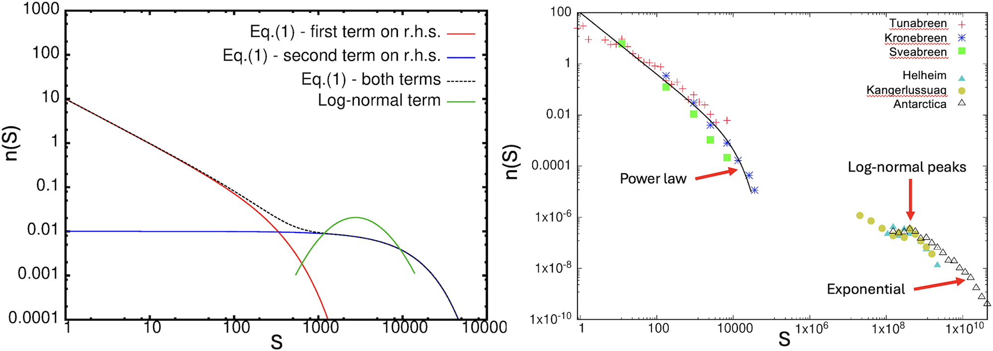
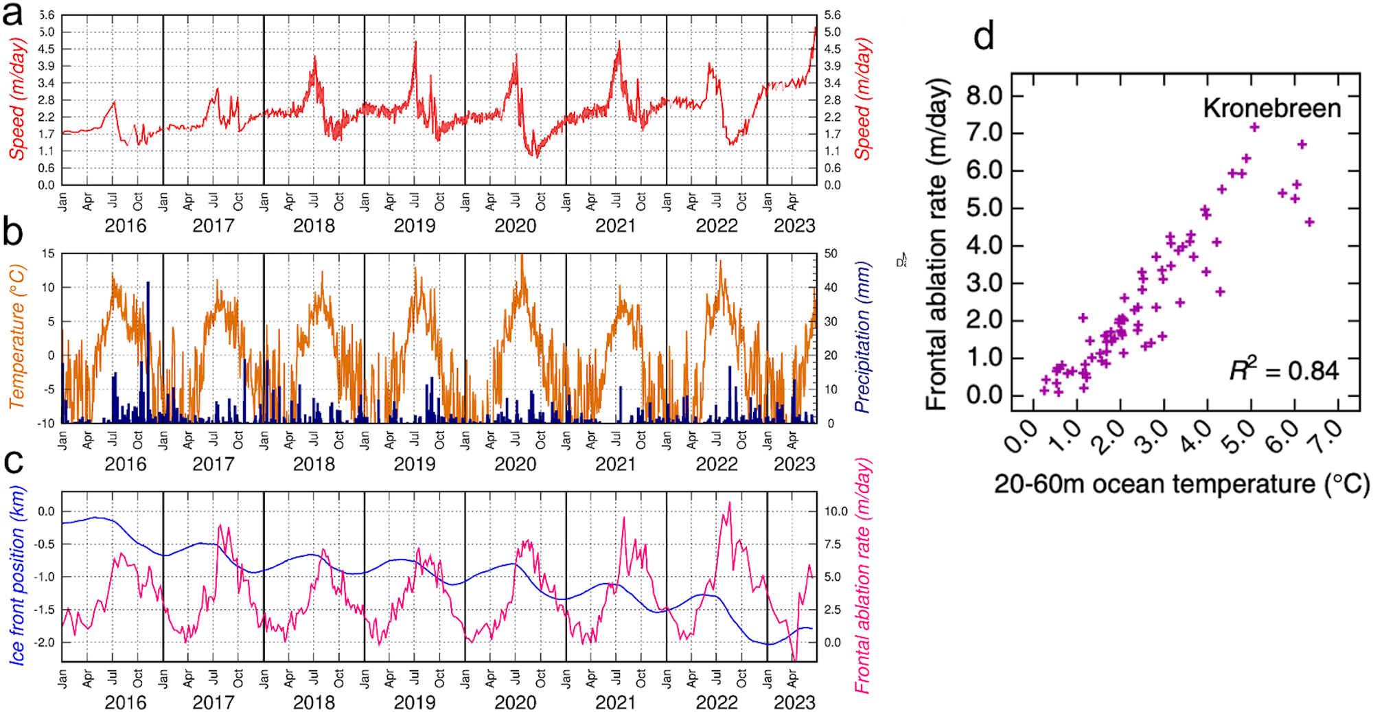
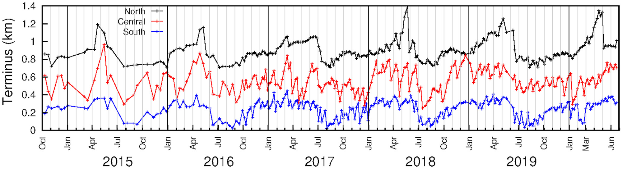
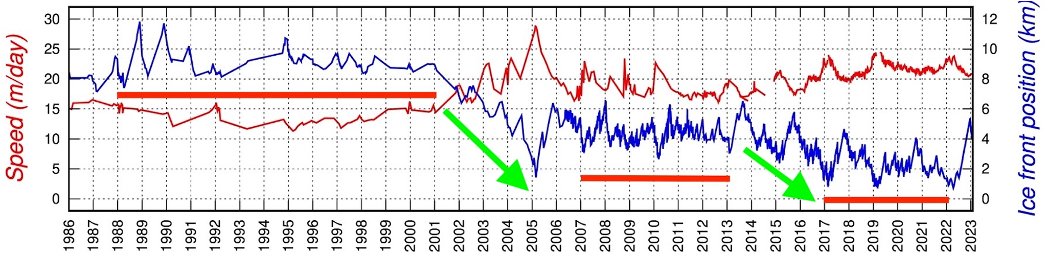
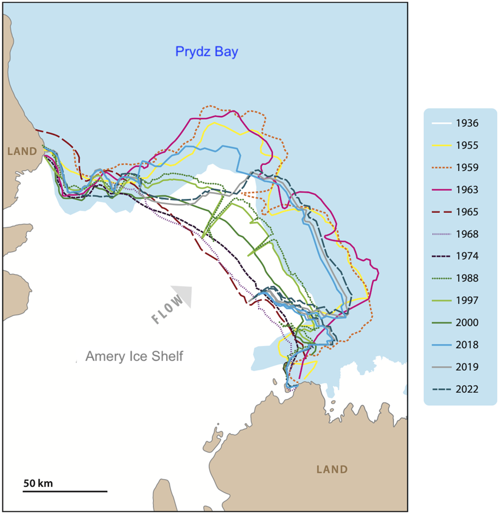
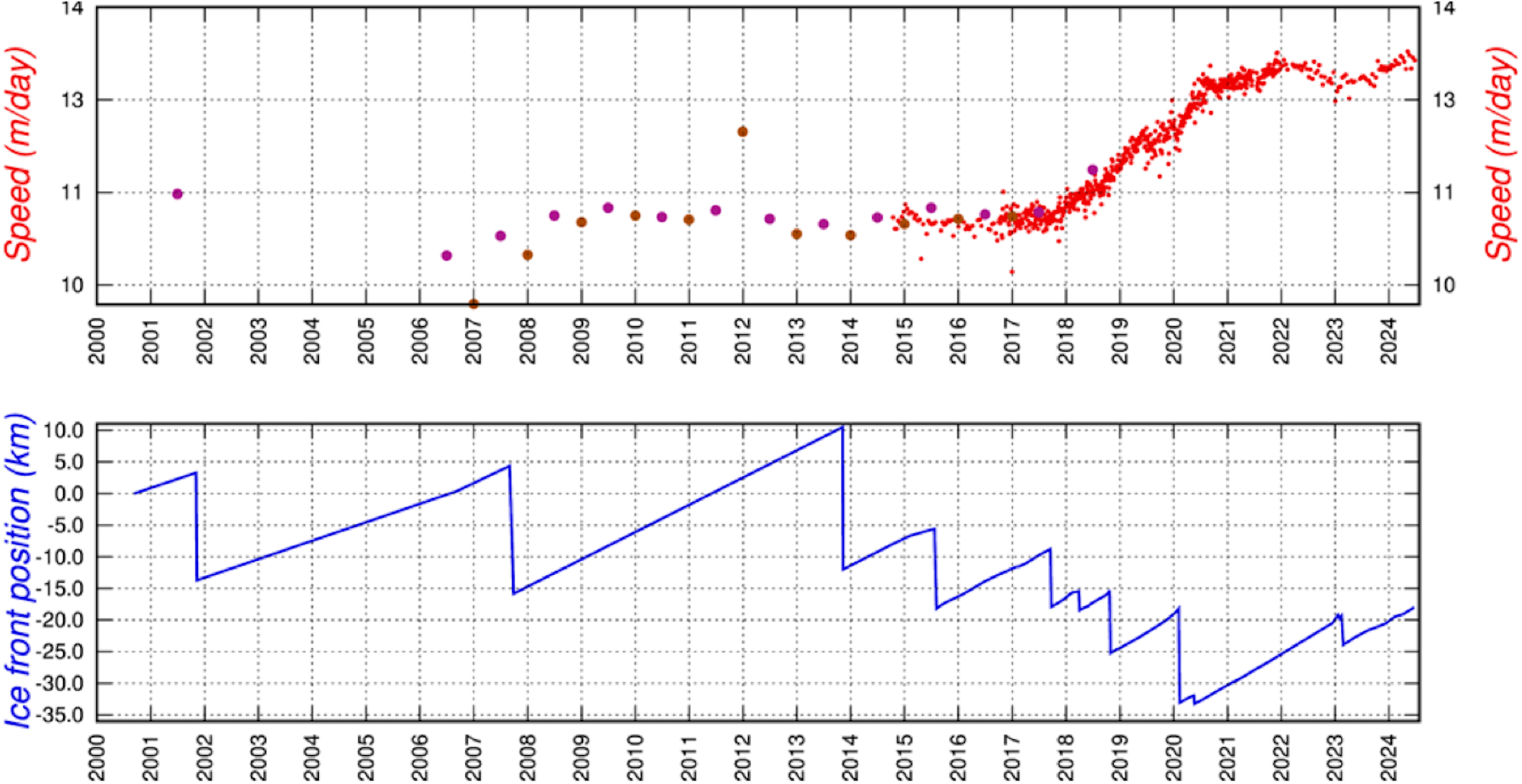
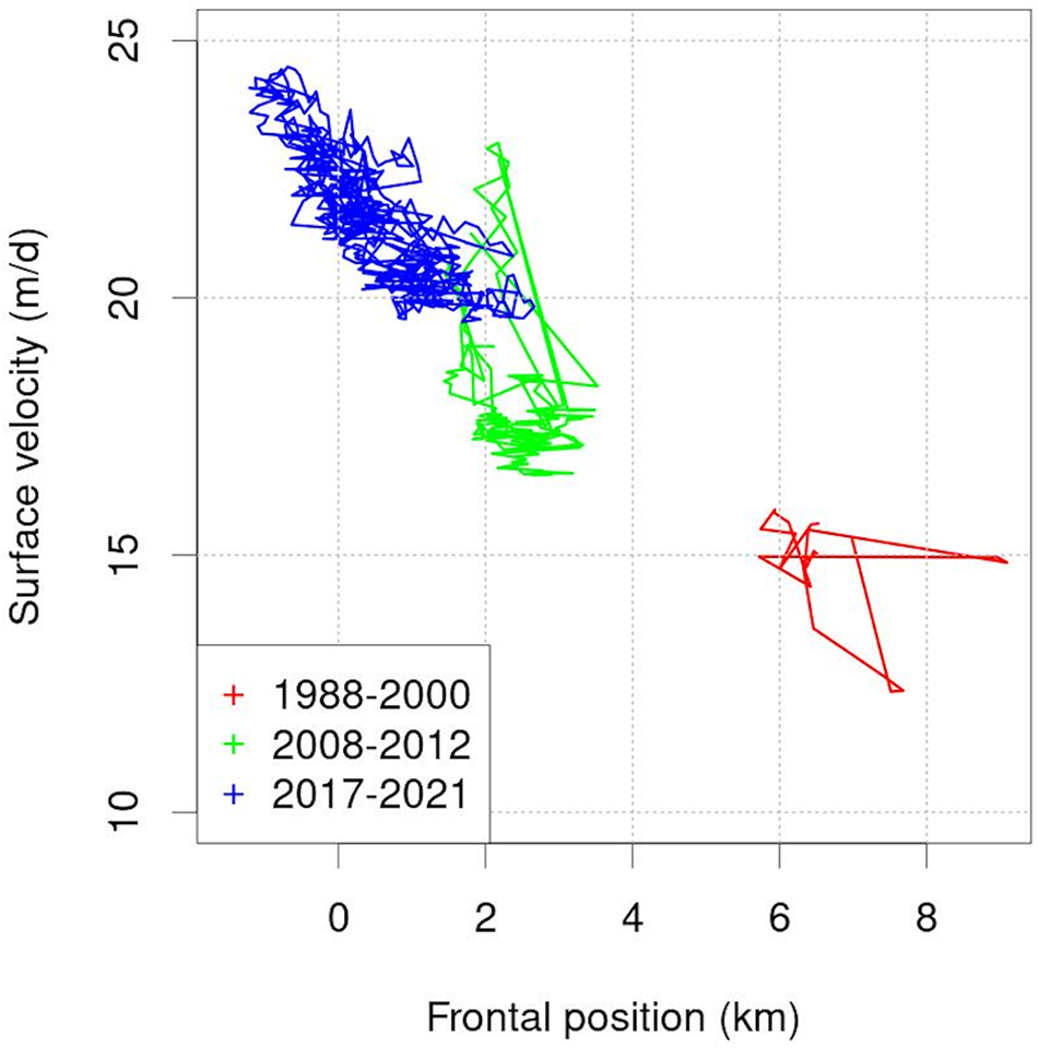
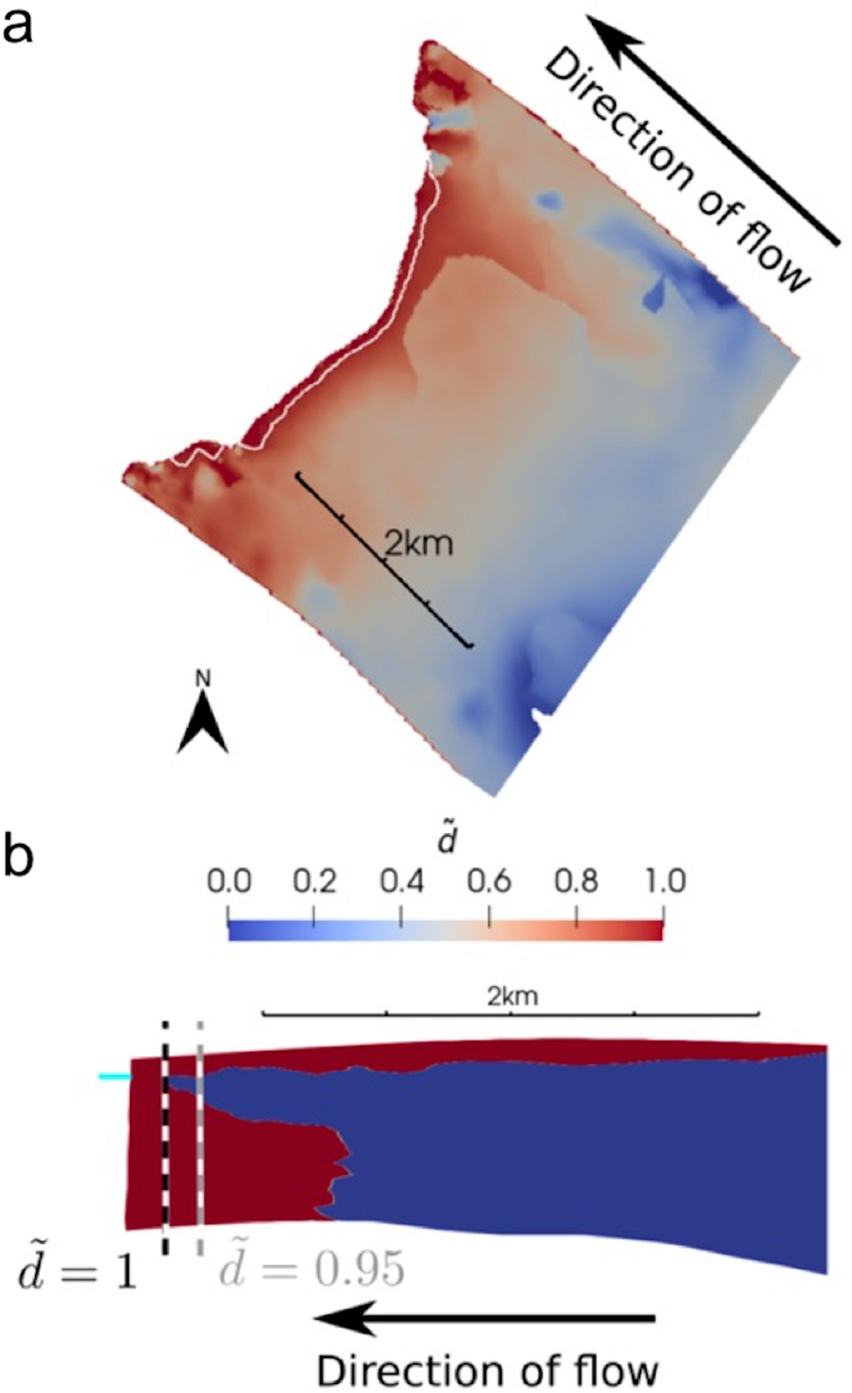


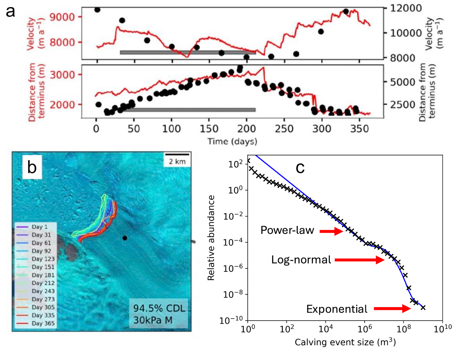


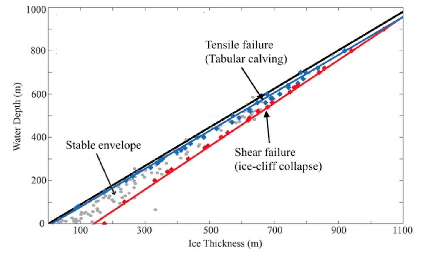
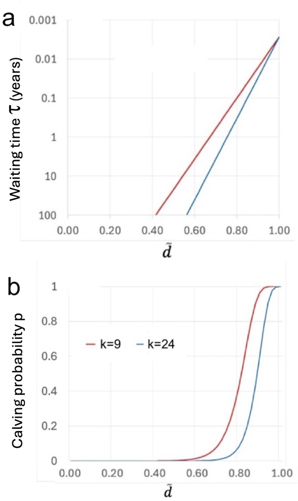


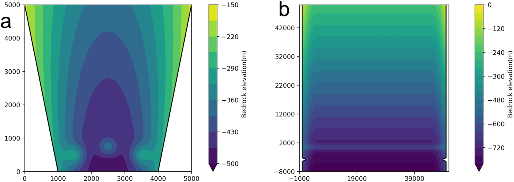
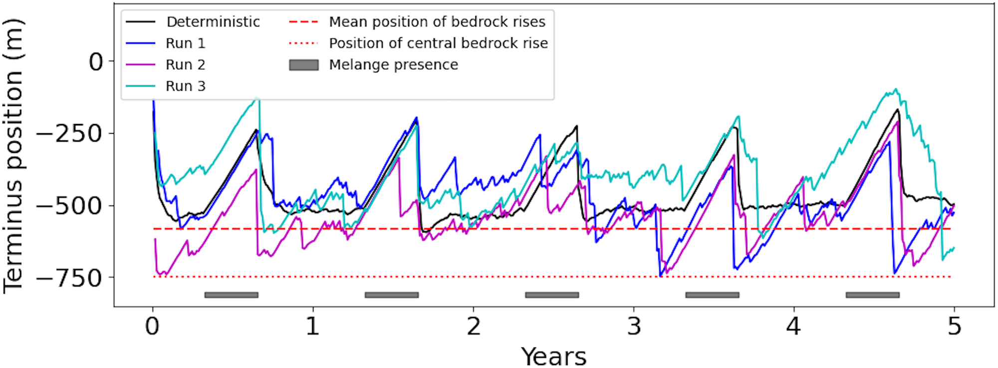

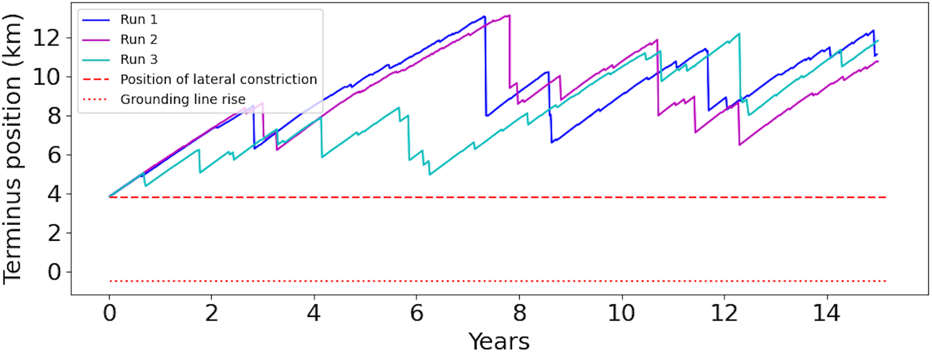
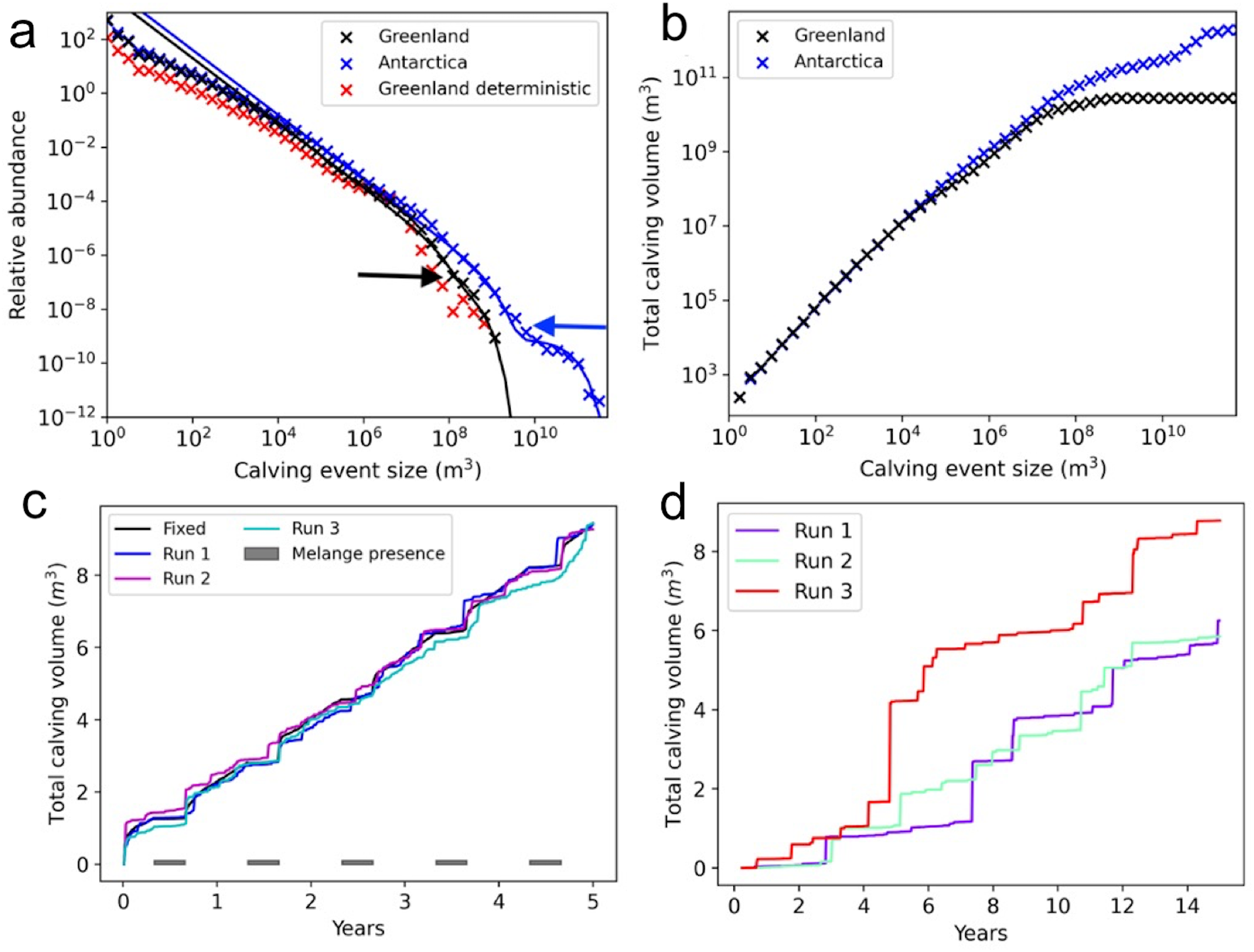


 Open access