

1 INTRODUCTION
In this article, we consider the instrumental variables (IV) estimation of a dynamic panel autoregressive (AR) process of possibly infinite order in the presence of individual effects. An infinite order panel AR process is a general specification in that it can include various linear time-series processes, such as stationary and invertible panel AR-moving-average (ARMA) models with individual effects. In addition, it does not require prespecification of the lag order, and thus is less subject to problems caused by possible model misspecification. It can then be applied to several important issues, including the estimation of the long-run cumulative effect of productivity shocks or demand shocks on the economy.
We consider a class of estimators that rely on the IV approach. Lee, Okui, and Shintani (Reference Lee, Okui and Shintani2018) consider the fixed effects (FE) estimation of infinite order panel AR models. However, their approach requires long time series, and many panel data sets encompass large cross sections and relatively short time periods. IV estimators, originally developed for short panels, are expected to behave well when the time series is not very long. In this article, we consider the following three types of IV estimators, namely, i) the IV estimator of Anderson and Hsiao (Reference Anderson and Hsiao1981, Reference Anderson and Hsiao1982); ii) the generalized methods of moments (GMM) estimator of Holtz-Eakin, Newey, and Rosen (Reference Holtz-Eakin, Newey and Rosen1988) and Arellano and Bond (Reference Arellano and Bond1991); and iii) the double filter IV (DFIV) estimator of Hayakawa (Reference Hayakawa2009).
Since the seminal work of Anderson and Hsiao (Reference Anderson and Hsiao1981, Reference Anderson and Hsiao1982), IV methods have been widely used for the estimation of dynamic panel data models.Footnote 1 This is because IV methods provide consistent estimators for panel AR processes with finite lag order, even when T, the length of time series, is fixed. The Anderson–Hsiao (AH) estimator is based on the first difference equation and employs the second-order lagged dependent variable as an instrument. Holtz-Eakin et al. (Reference Holtz-Eakin, Newey and Rosen1988) and Arellano and Bond (Reference Arellano and Bond1991) propose the use of the GMM estimator, which specifies all lagged variables as instruments, to improve efficiency.
Among these estimators, the GMM estimator is arguably the most popular estimator for dynamic panel data models. However, it is also known that the GMM estimator suffers from bias caused by the presence of many moment conditions in finite samples (Alvarez and Arellano, Reference Alvarez and Arellano2003; Newey and Smith, Reference Newey and Smith2004; Okui, Reference Okui2009).
To avoid this “many-moment bias,” Hayakawa (Reference Hayakawa2009) suggests an estimator based on the observation that the optimal instrument can be approximated by the difference between the lagged dependent variable and the average of all lags in a large T. This estimator is named the DFIV estimator by Hayakawa, Qi, and Breitung (Reference Hayakawa, Qi and Breitung2019). The DFIV estimator offers an estimator that is efficient when T tends to infinity, does not suffer from many-moment bias because it uses only a small number of instruments, and is consistent even when T is fixed because it is an IV estimator.
We extend the IV approaches, which are developed for panel AR processes with finite lag order, to infinite order panel AR models. Our approach is to approximate the infinite order panel AR model using a finite order panel AR model, and then estimate the model with finite lag order. The advantage of the sieve AR approximation is computational simplicity because it allows us to apply the existing estimators with little modification and the statistical software and packages used to compute these estimators are readily available.Footnote 2 The IV estimation of panel AR models with infinite order has not been considered in the literature and theoretical justification of the proposed methods is needed.
We establish the asymptotic properties of the AH, GMM, and DFIV estimators for an infinite order AR model with individual effects when both cross-sectional sample size N and time-series length T tend to infinity under homoskedasticity. We show that all three estimators are consistent and asymptotically normal. The GMM and DFIV estimators have a common asymptotic variance, while the AH estimator exhibits a different asymptotic variance and is less efficient. Moreover, the AH estimator may have a slower rate of convergence. We note that the asymptotic normality of the GMM estimator is derived under the assumption of N growing at a rate faster than T. If this assumption does not hold, “many-moment bias” will not be asymptotically negligible, and the asymptotic distribution of the GMM estimator would not be centered around zero. The asymptotic normality of the AH estimator also requires that N grows at a rate sufficiently faster than T.
In contrast, the asymptotic normality of the DFIV estimator does not require any condition on the relative rate of growth for N and T. Thus, we can expect that the DFIV estimator may behave better than the GMM estimator when T is not very small. Indeed, in a Monte Carlo simulation, the DFIV estimator performs better than the GMM estimator in terms of bias and the coverage of the confidence interval. For these reasons, the DFIV estimator is our preferred estimator for finite samples.
We also explore extensions and lag-order selection for the DFIV estimators. First, we extend our analysis to models that include exogenous regressors, demonstrating the asymptotic properties of our preferred DFIV estimator in these cases. Second, while we consider homoskedastic error terms in the theoretical analysis, we develop cluster-robust standard errors for the DFIV estimator to accommodate possibly heteroskedastic and correlated errors. Third, we determine the lag order using a general-to-specific approach, as outlined by Ng and Perron (Reference Ng and Perron1995). We demonstrate that this lag selection procedure can yield a lag order that satisfies the conditions required for asymptotic normality.
In the time-series literature, the issue of estimating infinite order AR models has a long tradition. For example, Berk (Reference Berk1974) considers the estimation of the spectral density of a univariate infinite order AR process, and Lewis and Reinsel (Reference Lewis and Reinsel1985) generalize the univariate results in Berk (Reference Berk1974) to the problem of multivariate prediction. Both Berk (Reference Berk1974) and Lewis and Reinsel (Reference Lewis and Reinsel1985) consider the sieve AR approximation to propose a nonparametric approach and estimate the approximated model using the least squares estimator. The present article also considers the sieve AR approximation but differs in that we focus on panel data with large cross sections and short or moderate length time series.
The estimation of dynamic panel data models has been extensively discussed in the literature (see, e.g., Bun and Sarafidis, Reference Bun and Sarafidis2015 for a review). However, most existing studies consider finite order panel AR models. An exception is Lee et al. (Reference Lee, Okui and Shintani2018) who recently consider the FE estimation of infinite order panel AR models. Their approach requires a relatively large T, whereas this article focuses on cases with large cross sections and time series of either relatively short or moderate length. In this sense, our article complements Lee et al. (Reference Lee, Okui and Shintani2018). Furthermore, the article considers a more general model with a finite number of exogenous regressors.
Our method addresses key empirical questions, especially in panel datasets with a large cross-sectional dimension (N), as is common in micro-panel studies. While the FE estimator of Lee et al. (Reference Lee, Okui and Shintani2018) is suitable when the time dimension (T) is large, our approach offers distinct advantages when N is large. This feature makes our method particularly valuable for several empirical applications: estimating long-run effects of productivity or demand shocks, measuring persistence via the sum of AR coefficients (SAR), and analyzing the speed of price adjustment toward the law of one price across U.S. city pairs (Crucini, Shintani, and Tsuruga, Reference Crucini, Shintani and Tsuruga2015). Our method is also well-suited for estimating the speed of adjustment of firms’ leverage toward target levels in capital structure research (Chang and Dasgupta, Reference Chang and Dasgupta2009; Dang, Kim, and Shin, Reference Dang, Kim and Shin2015). Furthermore, by leveraging the infinite order AR representation of ARMA processes, our approach enables flexible analysis of income dynamics, persistence, and adjustment without restrictive lag specifications (Nakata and Tonetti, Reference Nakata and Tonetti2015).
The DFIV estimator, our preferred estimator, was originally proposed by Hayakawa (Reference Hayakawa2009) for finite order AR models. It has since been extended to various other cases: Hayakawa (Reference Hayakawa2016) extends it to (finite order) panel vector AR models and Hayakawa, Qi, and Breitung (Reference Hayakawa, Qi and Breitung2019) to other types of (finite order) dynamic panel data models, including heterogeneous time trends models. This article provides a further extension of the DFIV estimator, illustrating its continued usefulness.
The remainder of this article is organized as follows. Section 2 describes the model. The AH, GMM and DFIV estimators are introduced in Section 3, where we also derive their asymptotic properties. The finite-sample performance of these estimators is examined in Section 4. Finally, Section 5 provides some concluding remarks. The mathematical proofs are in the mathematical appendix. The Supplementary Material contains the proofs of some technical lemmas.
We use the following notation: For a sequence of vectors $a_{it}$
, we let
$a_{it}$
, we let $a_{t}=(a_{1t},\dots ,a_{Nt})^{\prime }$
. The same convention applies to a sequence of vectors denoted by
$a_{t}=(a_{1t},\dots ,a_{Nt})^{\prime }$
. The same convention applies to a sequence of vectors denoted by $a_{it} (p)$
so that
$a_{it} (p)$
so that $a_{t} (p) = (a_{1t} (p), \dots , a_{Nt} (p))^{\prime }$
. For a vector l,
$a_{t} (p) = (a_{1t} (p), \dots , a_{Nt} (p))^{\prime }$
. For a vector l, $|| l ||$
denotes its Euclidean norm, that is,
$|| l ||$
denotes its Euclidean norm, that is, $||l||=(l^{\prime }l)^{1/2}$
.
$||l||=(l^{\prime }l)^{1/2}$
. $\to _p$
and
$\to _p$
and $\to _d$
signify convergence in probability and convergence in distribution, respectively.
$\to _d$
signify convergence in probability and convergence in distribution, respectively.
2 THE MODEL
We assume that panel data $\{ \{y_{it}\}_{t=1}^{T}\}_{i=1}^{N}$
are generated from an AR process of possibly infinite order with individual specific effects:
$\{ \{y_{it}\}_{t=1}^{T}\}_{i=1}^{N}$
are generated from an AR process of possibly infinite order with individual specific effects:
 $$ \begin{align} y_{it}=\mu_{i}+\sum_{k=1}^{\infty }\alpha _{k}y_{i,t-k}+\epsilon _{it}, \end{align} $$
where i and t denote the individual and period, respectively, $\mu _{i}$
is an unobservable individual effect for individual i to capture the heterogeneity across individuals,
$\mu _{i}$
is an unobservable individual effect for individual i to capture the heterogeneity across individuals, $\alpha _k$
is the coefficient on the kth lag, and
$\alpha _k$
is the coefficient on the kth lag, and $\epsilon _{it}$
is an unobservable innovation with mean zero and variance
$\epsilon _{it}$
is an unobservable innovation with mean zero and variance $\sigma ^{2}$
.Footnote
3
The stationarity of
$\sigma ^{2}$
.Footnote
3
The stationarity of $y_{it}$
is imposed throughout the analysis. The specification (1) is quite general and can include various linear stationary time series. A more general specification with exogenous regressors is considered in the later section. We also introduce an infinite order moving average representation of (1):
$y_{it}$
is imposed throughout the analysis. The specification (1) is quite general and can include various linear stationary time series. A more general specification with exogenous regressors is considered in the later section. We also introduce an infinite order moving average representation of (1):
 $$ \begin{align*} y_{it}=\eta _{i}+\sum_{k=0}^{\infty }\psi _{k}\epsilon _{i,t-k}, \end{align*} $$
where $\psi _{0}\equiv 1$
and
$\psi _{0}\equiv 1$
and $ \eta _{i}=\mu _{i}/(1-\sum _{k=1}^{\infty }\alpha _{k})$
.Footnote
4
$ \eta _{i}=\mu _{i}/(1-\sum _{k=1}^{\infty }\alpha _{k})$
.Footnote
4
We employ the following assumptions throughout the article.
Assumption 1. (i) $\{ \epsilon _{it}\}$
are independently and identically distributed (i.i.d.) over time and across individuals with mean zero,
$\{ \epsilon _{it}\}$
are independently and identically distributed (i.i.d.) over time and across individuals with mean zero, $0<E(\epsilon _{it}^{2})=\sigma ^{2}<\infty $
and
$0<E(\epsilon _{it}^{2})=\sigma ^{2}<\infty $
and $E|\epsilon _{it}|^{2r}\leq C_1,r>2$
for some constant
$E|\epsilon _{it}|^{2r}\leq C_1,r>2$
for some constant $C_1>0$
and
$C_1>0$
and $\{\mu _i\}$
are i.i.d. across individuals with
$\{\mu _i\}$
are i.i.d. across individuals with $E(\mu _i^2)<C_2$
for some constant
$E(\mu _i^2)<C_2$
for some constant $C_2>0$
; (ii)
$C_2>0$
; (ii) $\epsilon _{it}$
is independent of
$\epsilon _{it}$
is independent of $\mu _{i}$
for all i and t; (iii)
$\mu _{i}$
for all i and t; (iii) $\sum _{k=1}^{\infty }|\alpha _{k}|<\infty $
and
$\sum _{k=1}^{\infty }|\alpha _{k}|<\infty $
and $ 1- \sum _{k=1}^{\infty }\alpha _{k}z^{k} \neq 0$
for any
$ 1- \sum _{k=1}^{\infty }\alpha _{k}z^{k} \neq 0$
for any $|z|\leq 1$
; and (iv)
$|z|\leq 1$
; and (iv) $y_{i,1-s} $
,
$y_{i,1-s} $
, $s=0,1,2,\dots $
, are generated from the stationary distribution given
$s=0,1,2,\dots $
, are generated from the stationary distribution given $\mu _i$
.
$\mu _i$
.
In Assumption 1(i), we restrict our attention to cases with i.i.d. error $\{ \epsilon _{it}\}$
to simplify our mathematical arguments. Alternatively, we can relax the independence assumption to, for example, a martingale difference sequence at the cost of imposing stronger moment conditions and resulting in more complicated mathematical derivations. In contrast, relaxing the homoskedasticity assumption may have an important consequence for our results regarding the GMM estimator as in the case of the panel AR(1) model in Alvarez and Arellano (Reference Alvarez and Arellano2003).Footnote
5
We recognize that heteroskedasticity is an important concern in real applications. For the DFIV estimator, we introduce cluster-robust standard errors that account for heteroskedasticity in Section 3.5. Assumption 1(ii) is used for the moving average representation of the model and also for the validity of the moment conditions used in the GMM estimator. Assumption 1(iii) indicates that
$\{ \epsilon _{it}\}$
to simplify our mathematical arguments. Alternatively, we can relax the independence assumption to, for example, a martingale difference sequence at the cost of imposing stronger moment conditions and resulting in more complicated mathematical derivations. In contrast, relaxing the homoskedasticity assumption may have an important consequence for our results regarding the GMM estimator as in the case of the panel AR(1) model in Alvarez and Arellano (Reference Alvarez and Arellano2003).Footnote
5
We recognize that heteroskedasticity is an important concern in real applications. For the DFIV estimator, we introduce cluster-robust standard errors that account for heteroskedasticity in Section 3.5. Assumption 1(ii) is used for the moving average representation of the model and also for the validity of the moment conditions used in the GMM estimator. Assumption 1(iii) indicates that $y_{it}$
is stationary and can be represented by an infinite order moving average process. We note that the violation of
$y_{it}$
is stationary and can be represented by an infinite order moving average process. We note that the violation of $p^{1/2}\sum _{k=p+1}^{\infty } \alpha _k \rightarrow 0$
does not necessarily imply the violation of Assumption 1(iii).Footnote
6
Assumption 1(iv) is an assumption about the initial observation, which can be relaxed as the influence of the initial observations diminishes when T is sufficiently large. We impose this assumption to avoid tedious mathematical arguments.
$p^{1/2}\sum _{k=p+1}^{\infty } \alpha _k \rightarrow 0$
does not necessarily imply the violation of Assumption 1(iii).Footnote
6
Assumption 1(iv) is an assumption about the initial observation, which can be relaxed as the influence of the initial observations diminishes when T is sufficiently large. We impose this assumption to avoid tedious mathematical arguments.
3 INSTRUMENTAL VARIABLES APPROACH
Our estimation strategy for the model is based on the IV approach originated by Anderson and Hsiao (Reference Anderson and Hsiao1981). Note that in general, least squares or maximum likelihood estimation of dynamic panel data models does not yield a consistent estimator because of the presence of individual effects when T is fixed. When T tends to infinity, such an estimator would be consistent but would suffer from considerable bias (see, e.g., Hahn and Kuersteiner, Reference Hahn and Kuersteiner2002; Alvarez and Arellano, Reference Alvarez and Arellano2003; Lee et al. Reference Lee, Okui and Shintani2018). IV estimators are attractive because of the following reasons. First, when the approximated model is correct, the IV estimators are consistent even when T is fixed. Second, we expect smaller bias when N is large relative to T.
To estimate (1), we consider the following approximated model:
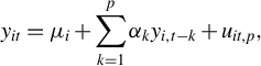 $$ \begin{align} y_{it}=\mu _{i}+\sum_{k=1}^{p}\alpha _{k}y_{i,t-k}+u_{it,p}, \end{align} $$
where $u_{it,p}=b_{it,p}+\epsilon _{it}$
with the “truncation error”
$u_{it,p}=b_{it,p}+\epsilon _{it}$
with the “truncation error” $b_{it,p}=\sum _{k=p+1}^{\infty }\alpha _{k}y_{i,t-k}$
. This truncation error arises due to approximating the true infinite order AR model in (1) by the AR model with a truncated lag, p, in (2). The choice of p is discussed in Section 3.8. The advantage of considering the approximated model (2) lies in the computational tractability of the parametric finite order AR model while the effect of model misspecification disappears asymptotically. Note that while the error term
$b_{it,p}=\sum _{k=p+1}^{\infty }\alpha _{k}y_{i,t-k}$
. This truncation error arises due to approximating the true infinite order AR model in (1) by the AR model with a truncated lag, p, in (2). The choice of p is discussed in Section 3.8. The advantage of considering the approximated model (2) lies in the computational tractability of the parametric finite order AR model while the effect of model misspecification disappears asymptotically. Note that while the error term $u_{it,p}$
in the approximating model is heteroskedastic, we do not need to be concerned about the heteroskedasticity resulting from truncation or approximation error
$u_{it,p}$
in the approximating model is heteroskedastic, we do not need to be concerned about the heteroskedasticity resulting from truncation or approximation error $b_{it,p}=\sum _{k=p+1}^{\infty } \alpha _k y_{i,t-k}$
. Nonetheless, to circumvent a concern in finite samples, we provide heteroskedasticity-robust standard error formulas for the DFIV estimator in Section 3.5. In each theorem below, we impose conditions on
$b_{it,p}=\sum _{k=p+1}^{\infty } \alpha _k y_{i,t-k}$
. Nonetheless, to circumvent a concern in finite samples, we provide heteroskedasticity-robust standard error formulas for the DFIV estimator in Section 3.5. In each theorem below, we impose conditions on $\sum _{k=p+1}^{\infty }{|\alpha _k|}$
to ensure that the truncation error does not affect the asymptotic analyses. To estimate parameters in the approximated model (2), we consider three estimators from the class of IV estimators in the following sections.
$\sum _{k=p+1}^{\infty }{|\alpha _k|}$
to ensure that the truncation error does not affect the asymptotic analyses. To estimate parameters in the approximated model (2), we consider three estimators from the class of IV estimators in the following sections.
3.1 The Anderson–Hsiao Estimator
The first estimator we consider relies on the approach taken by Anderson and Hsiao (Reference Anderson and Hsiao1981, Reference Anderson and Hsiao1982), which is based on the first difference equation. In this section, we provide the asymptotic properties of the AH estimator.
The first step in the AH estimator is to eliminate the individual effects using first differences. Let us rewrite the approximated model (2) by
 $$ \begin{align*} y_{it}=\mu _{i}+x_{it}(p)^{\prime }\alpha (p)+u_{it,p} , \end{align*} $$
where $x_{it}(p)=(y_{i,t-1},\ldots ,y_{i,t-p})^{\prime }$
and
$x_{it}(p)=(y_{i,t-1},\ldots ,y_{i,t-p})^{\prime }$
and $ \alpha (p)=( \alpha _{1},\ldots ,\alpha _{p})^{\prime } $
. Differencing to remove the individual specific effect
$ \alpha (p)=( \alpha _{1},\ldots ,\alpha _{p})^{\prime } $
. Differencing to remove the individual specific effect $\mu _{i}$
yields
$\mu _{i}$
yields
 $$ \begin{align} \Delta y_{it}=\alpha (p)^{\prime }\Delta x_{it}(p)+\Delta u_{it,p}, \end{align} $$
where $\Delta $
is the difference operator so that
$\Delta $
is the difference operator so that $\Delta y_{it}=y_{it}-y_{i,t-1}$
,
$\Delta y_{it}=y_{it}-y_{i,t-1}$
, $\Delta x_{it} (p) = x_{it} (p) - x_{i,t-1} (p),$
and
$\Delta x_{it} (p) = x_{it} (p) - x_{i,t-1} (p),$
and $\Delta u_{it} = u_{it} - u_{i,t-1}$
.
$\Delta u_{it} = u_{it} - u_{i,t-1}$
.
The AH estimator is based on the following moment conditions. For $\Delta \epsilon _{it} = \epsilon _{it} - \epsilon _{i,t-1}$
,
$\Delta \epsilon _{it} = \epsilon _{it} - \epsilon _{i,t-1}$
,
 $$ \begin{align*} E(y_{i,t-s}\Delta \epsilon _{it})=0\text{ for }2\leq s\leq p+1 \text{ and } t= p+2, \dots, T. \end{align*} $$
For each t, there are p moment conditions. Because the dimension of $\alpha (p)$
is p, there are as many moment conditions as the parameters for each t. Given we cannot recover
$\alpha (p)$
is p, there are as many moment conditions as the parameters for each t. Given we cannot recover $\Delta \epsilon _{it}$
because of
$\Delta \epsilon _{it}$
because of $b_{it}$
, we use
$b_{it}$
, we use $\Delta u_{it}$
, although this yields moment conditions that are only approximately valid. Solving the sample analog of the set of moment conditions, we obtain the AH estimator:
$\Delta u_{it}$
, although this yields moment conditions that are only approximately valid. Solving the sample analog of the set of moment conditions, we obtain the AH estimator:
 $$ \begin{align*} \hat{\alpha}_{AH}(p)=\left( \sum_{i=1}^{N} \sum_{t=p+2}^T Z_{it}(p)\Delta x_{it}^{\prime }(p)\right) ^{-1}\sum_{i=1}^{N} \sum_{t=p+2}^T Z_{it}(p)\Delta y_{it}, \end{align*} $$
where $Z_{it}(p)=(y_{i,t-2}, \dots , y_{i,t-p-1})^{\prime }$
.
$Z_{it}(p)=(y_{i,t-2}, \dots , y_{i,t-p-1})^{\prime }$
.
We make the following additional assumption to analyze the asymptotic properties of the estimator. Let $\gamma _{j}=E(w_{it} w_{i,t-j})$
, where
$\gamma _{j}=E(w_{it} w_{i,t-j})$
, where $w_{it}=y_{it}-\eta _{i}=\sum _{k=0}^{\infty }\psi _{k}\epsilon _{i,t-k}$
. Define
$w_{it}=y_{it}-\eta _{i}=\sum _{k=0}^{\infty }\psi _{k}\epsilon _{i,t-k}$
. Define
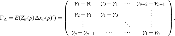 $$ \begin{align*} \Gamma _{\Delta }=E(Z_{it}(p)\Delta x_{it}(p)^{\prime })=\left( \begin{array}{cccc} \gamma _{1}-\gamma _{0} & \gamma _{0}-\gamma _{1} & \cdots & \gamma _{p-2}-\gamma _{p-1} \\ \gamma _{2}-\gamma _{1} & \gamma _{1}-\gamma _{0} & & \vdots \\ \vdots & & \ddots & \vdots \\ \gamma _{p}-\gamma _{p-1} & \cdots & \cdots & \gamma_{1}-\gamma _{0} \end{array} \right). \end{align*} $$
Assumption 2. $\Gamma _{\Delta }$
is invertible for any p. The square root of the largest eigenvalue of
$\Gamma _{\Delta }$
is invertible for any p. The square root of the largest eigenvalue of $\Gamma _{\Delta }^{-1\prime }\Gamma _{\Delta }^{-1}$
, denoted by
$\Gamma _{\Delta }^{-1\prime }\Gamma _{\Delta }^{-1}$
, denoted by $\lambda _p$
, is finite for any p.
$\lambda _p$
, is finite for any p.
The invertibility requires that the process is not too persistent. Section 9 of the Supplementary Material demonstrates the invertibility when $w_{it}$
is an i.i.d. process. Typically,
$w_{it}$
is an i.i.d. process. Typically, $\lambda _p$
is
$\lambda _p$
is $O(\sqrt {p})$
and
$O(\sqrt {p})$
and $\lambda _p>1$
, in general with
$\lambda _p>1$
, in general with $p>1$
. In Section 9 of the Supplementary Material, we derive the exact value of
$p>1$
. In Section 9 of the Supplementary Material, we derive the exact value of $\lambda _p$
in a simple case. Note that this assumption allows
$\lambda _p$
in a simple case. Note that this assumption allows $\lambda _p$
to explode as
$\lambda _p$
to explode as $p\to \infty $
.
$p\to \infty $
.
We first prove the consistency of $\hat {\alpha }_{AH}(p)$
.
$\hat {\alpha }_{AH}(p)$
.
Theorem 1. Suppose that Assumptions 1 and 2 are satisfied. If $N\rightarrow \infty $
,
$N\rightarrow \infty $
, $T -p\rightarrow \infty , $
and
$T -p\rightarrow \infty , $
and $p\to \infty $
with
$p\to \infty $
with $\lambda _p \sqrt {p} \sum _{k=p+1}^{\infty } |\alpha _k | \to 0$
and
$\lambda _p \sqrt {p} \sum _{k=p+1}^{\infty } |\alpha _k | \to 0$
and $\lambda _p^2 p^2 / (N (T-p)) \to 0$
, we have
$\lambda _p^2 p^2 / (N (T-p)) \to 0$
, we have
 $$ \begin{align*} ||\hat{\alpha}_{AH}(p)-\alpha (p)||\rightarrow _{p}0. \end{align*} $$
Next, we show the asymptotic normality of a linear combination of the estimated AR parameters. Let $\ell _{p}$
be an arbitrary sequence of
$\ell _{p}$
be an arbitrary sequence of $p\times 1$
vectors such that
$p\times 1$
vectors such that $0<M_{1}\leq ||\ell _{p}||^{2}=\ell _{p}^{\prime }\ell _{p}\leq M_{2}<\infty $
, for some constants
$0<M_{1}\leq ||\ell _{p}||^{2}=\ell _{p}^{\prime }\ell _{p}\leq M_{2}<\infty $
, for some constants $M_1, M_2>0$
.
$M_1, M_2>0$
.
Theorem 2. Suppose that Assumptions 1 and 2 are satisfied. If $N\rightarrow \infty $
,
$N\rightarrow \infty $
, $T -p \rightarrow \infty , $
and
$T -p \rightarrow \infty , $
and $p\to \infty $
with
$p\to \infty $
with $(T-p) \lambda _p^2 p / N^2 =O(1)$
,
$(T-p) \lambda _p^2 p / N^2 =O(1)$
, $\lambda _p^4 p^4 / (N(T-p)) \to 0$
,
$\lambda _p^4 p^4 / (N(T-p)) \to 0$
, $\lambda _p \sqrt {N(T-p)p} \sum _{k=p+1}^{\infty } |\alpha _k | \to 0 $
, and
$\lambda _p \sqrt {N(T-p)p} \sum _{k=p+1}^{\infty } |\alpha _k | \to 0 $
, and $\lambda _p^2 p^{3/2} \sum _{k=p+1}^{\infty } |\alpha _k | \to 0$
, we have
$\lambda _p^2 p^{3/2} \sum _{k=p+1}^{\infty } |\alpha _k | \to 0$
, we have
 $$ \begin{align*} \sqrt{N(T-p)}\left[ \ell_{p}^{\prime }\hat{\alpha}_{AH}(p)-\ell_{p}^{\prime }\alpha (p)\right] /v_{p,AH}\to_d N(0,1), \end{align*} $$
where $v_{p,AH}^{2}=\ell _{p}^{\prime }\Gamma _{\Delta }^{-1} B_p\Gamma _{\Delta }^{-1} \ell _p$
and
$v_{p,AH}^{2}=\ell _{p}^{\prime }\Gamma _{\Delta }^{-1} B_p\Gamma _{\Delta }^{-1} \ell _p$
and $B_p=(T-p)^{-1} \sum _{t=p+2}^{T} \sum _{t'=\max (t-1,p+2)}^{\min (t+1,T)} E(\Delta \epsilon _{it}\Delta \epsilon _{it'} Z_{it}(p)Z_{it'}(p)^{\prime }) $
.
$B_p=(T-p)^{-1} \sum _{t=p+2}^{T} \sum _{t'=\max (t-1,p+2)}^{\min (t+1,T)} E(\Delta \epsilon _{it}\Delta \epsilon _{it'} Z_{it}(p)Z_{it'}(p)^{\prime }) $
.
The theorems require some conditions regarding the rates at which N and T tend to infinity. These conditions, in particular $(T-p) \lambda _p^2 p / N^2 =O(1)$
, imply that N should be sufficiently large compared with T. The requirement of large N is expected given that IV estimation for dynamic panel data models is originally developed to perform well when N is large but T is small. Note that
$(T-p) \lambda _p^2 p / N^2 =O(1)$
, imply that N should be sufficiently large compared with T. The requirement of large N is expected given that IV estimation for dynamic panel data models is originally developed to perform well when N is large but T is small. Note that $v_{p,AH}$
is of order
$v_{p,AH}$
is of order $\lambda _p$
and the convergence rate of the AH estimator is slower than
$\lambda _p$
and the convergence rate of the AH estimator is slower than $\sqrt {NT}$
. Roughly speaking, this slow convergence rate is caused by correlations across instruments which result in a weak set of moment conditions. The above theorem is established under
$\sqrt {NT}$
. Roughly speaking, this slow convergence rate is caused by correlations across instruments which result in a weak set of moment conditions. The above theorem is established under $T-p \to \infty $
. An inspection of the proof reveals that we need a different approach to handle the case with
$T-p \to \infty $
. An inspection of the proof reveals that we need a different approach to handle the case with $p=T$
. It is thus beyond the scope of the article.
$p=T$
. It is thus beyond the scope of the article.
We mainly examine conditions on N and T and let p be appropriately chosen when we discuss the asymptotic results, including those presented later. The empirical setting gives N and T, and they are not the choice of researchers. In contrast, p can be chosen. Thus, conditions on $ N $
and
$ N $
and $ T $
are more relevant to examining whether a particular method is applicable in a given setting.
$ T $
are more relevant to examining whether a particular method is applicable in a given setting.
3.2 The GMM Estimator
As the second IV estimator, we consider the GMM estimator based on Holtz-Eakin et al. (Reference Holtz-Eakin, Newey and Rosen1988) and Arellano and Bond (Reference Arellano and Bond1991). For the GMM estimator, we apply the forward filter to the variables to eliminate the individual effects.Footnote 7 Let
 $$ \begin{align*} y_{it}^{\ast }=\sqrt{\frac{T-t}{T-t+1}}\left( y_{it}-\frac{1}{T-t} (y_{i,t+1}+\dots +y_{iT})\right) , \end{align*} $$
and $x_{it}^{\ast }(p)$
and
$x_{it}^{\ast }(p)$
and $u_{it,p}^{\ast }$
be similarly defined.Footnote
8
In this article, a variable with
$u_{it,p}^{\ast }$
be similarly defined.Footnote
8
In this article, a variable with $ \ast $
superscript is a variable transformed by the forward filter even when it is not explicitly mentioned. By rewriting the model (2) in terms of the transformed variables, we have
$ \ast $
superscript is a variable transformed by the forward filter even when it is not explicitly mentioned. By rewriting the model (2) in terms of the transformed variables, we have
 $$ \begin{align} y_{it}^* = x_{it}^* (p)^{\prime }\alpha (p) + u_{it,p}^* \end{align} $$
so that the individual effect $\mu _{i}$
is eliminated.
$\mu _{i}$
is eliminated.
The GMM estimator exploits the following moment conditions:
 $$ \begin{align*} E(y_{i,t-s}\epsilon _{it}^{\ast })=0\text{ for }s\geq 1. \end{align*} $$
We note that there are $T-p-1$
equations (one equation for each period) to be estimated and the equation for
$T-p-1$
equations (one equation for each period) to be estimated and the equation for $y_{it}^{\ast }$
has
$y_{it}^{\ast }$
has $t-1$
instruments. Therefore, there are
$t-1$
instruments. Therefore, there are $\sum _{t=p+1}^{T-1}(t-1)=(T-2)(T-1)/2-(p-1)p/2$
moment conditions in total, and the number of moment conditions can be very large, even when T is not very large.
$\sum _{t=p+1}^{T-1}(t-1)=(T-2)(T-1)/2-(p-1)p/2$
moment conditions in total, and the number of moment conditions can be very large, even when T is not very large.
We now define the GMM estimator. Let $Z_{it}=(y_{i,t-1},\dots ,y_{i1})^{\prime }$
be the set of IV for the equation with
$Z_{it}=(y_{i,t-1},\dots ,y_{i1})^{\prime }$
be the set of IV for the equation with $y_{it}^{\ast }$
as the dependent variable. The GMM estimator,
$y_{it}^{\ast }$
as the dependent variable. The GMM estimator, $\hat {\alpha }_{G}(p)$
, is
$\hat {\alpha }_{G}(p)$
, is
 $$ \begin{align*} \hat{\alpha}_{G}(p)=\left( \sum_{t=p+1}^{T-1}x_{t}^{\ast }(p)^{\prime }M_{t}x_{t}^{\ast }(p)\right) ^{-1}\sum_{t=p+1}^{T-1}x_{t}^{\ast }(p)^{\prime }M_{t}y_{t}^{\ast }, \end{align*} $$
where $M_{t}=Z_{t}(Z_{t}^{\prime }Z_{t})^{-1}Z_{t}^{\prime }$
.
$M_{t}=Z_{t}(Z_{t}^{\prime }Z_{t})^{-1}Z_{t}^{\prime }$
.
To investigate the asymptotic properties of the GMM estimator, we employ the following two additional assumptions.
Assumption 3. $E(\mu _{i}^{4})$
is finite.
$E(\mu _{i}^{4})$
is finite.
Assumption 4. $\sum _{k=1}^{\infty } k |\psi _k| < \infty $
.
$\sum _{k=1}^{\infty } k |\psi _k| < \infty $
.
Assumption 3 imposes a tighter moment condition on individual effects. This assumption is used to control the variability of $ \sum _{t=p+1}^{T-1}x_{t}^{\ast }(p)^{\prime }M_{t}x_{t}^{\ast }(p)$
. Assumption 4 is satisfied, for example, when the true process is a finite order ARMA model. This assumption is employed to control the many-moment bias. The following theorem shows the consistency of
$ \sum _{t=p+1}^{T-1}x_{t}^{\ast }(p)^{\prime }M_{t}x_{t}^{\ast }(p)$
. Assumption 4 is satisfied, for example, when the true process is a finite order ARMA model. This assumption is employed to control the many-moment bias. The following theorem shows the consistency of $\hat {\alpha }_{G}(p)$
.
$\hat {\alpha }_{G}(p)$
.
Theorem 3. Suppose that Assumptions 1, 3, and 4 are satisfied. If $N \to \infty $
,
$N \to \infty $
, $T\to \infty ,$
and
$T\to \infty ,$
and $p\to \infty $
with
$p\to \infty $
with $T/N \to 0$
,
$T/N \to 0$
, $p^2 /T \to 0$
, and
$p^2 /T \to 0$
, and $ p^{1/2}\sum _{k=p+1}^{\infty }|\alpha _{k}|\rightarrow 0$
as
$ p^{1/2}\sum _{k=p+1}^{\infty }|\alpha _{k}|\rightarrow 0$
as $p\rightarrow \infty $
, we have
$p\rightarrow \infty $
, we have
 $$ \begin{align*} || \hat{\alpha}_G(p)-\alpha (p) || \to_p 0. \end{align*} $$
Next, we show the asymptotic normality of a linear combination of the estimated AR parameters. Let $v_{p}^{2}=\sigma ^{2}\ell _{p}^{\prime }\Gamma _{p}^{-1}\ell _{p}$
, where
$v_{p}^{2}=\sigma ^{2}\ell _{p}^{\prime }\Gamma _{p}^{-1}\ell _{p}$
, where
 $$ \begin{align*} \Gamma_p = \begin{pmatrix} \gamma_0 & \gamma_1 & \dots & \gamma_{p-1} \\ \gamma_1 & \gamma_0 & \dots & \gamma_{p-2} \\ \dots & \dots & \dots & \dots \\ \gamma_{p-1} & \gamma_{p-2} & \dots & \gamma_0 \end{pmatrix} \end{align*} $$
is the variance–covariance matrix of the vector $(w_{it},\dots ,w_{i,t-p+1})^{\prime }$
. Note that Assumption 1(iii) guarantees that the maximum eigenvalue of
$(w_{it},\dots ,w_{i,t-p+1})^{\prime }$
. Note that Assumption 1(iii) guarantees that the maximum eigenvalue of $\Gamma _p^{-1}$
is bounded, which implies that
$\Gamma _p^{-1}$
is bounded, which implies that $v_p^2$
is bounded away from zero. The following theorem provides the asymptotic normality of
$v_p^2$
is bounded away from zero. The following theorem provides the asymptotic normality of $\ell _{p}^{\prime }\hat {\alpha }_{G}(p)$
.
$\ell _{p}^{\prime }\hat {\alpha }_{G}(p)$
.
Theorem 4. Suppose that Assumptions 1, 3, and 4 are satisfied. If $N \to \infty $
,
$N \to \infty $
, $T\to \infty ,$
and
$T\to \infty ,$
and $p \to \infty $
with
$p \to \infty $
with $\sqrt {NT} \sum _{k=p+1}^{\infty }|\alpha _k| \to 0$
,
$\sqrt {NT} \sum _{k=p+1}^{\infty }|\alpha _k| \to 0$
,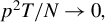 $p^2T /N \to 0, $
and
$p^2T /N \to 0, $
and $p^3 \log T /T \to 0 $
, we have
$p^3 \log T /T \to 0 $
, we have
 $$ \begin{align*} \sqrt{N(T-p)}\left[\ell_p^{\prime }\hat{\alpha}_G(p)-\ell_p^{\prime }\alpha (p) \right] /v_{p} \to_d N(0,1). \end{align*} $$
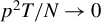
To assess the effect of an infinite lag order, we compare Theorem 4 with Theorem 2 of Alvarez and Arellano (Reference Alvarez and Arellano2003). The assumptions underlying our Theorem 4 are similar to those in their Theorem 2, which requires $N,T \to \infty $
,
$N,T \to \infty $
, $(\log T)^2 /N \to 0$
, and
$(\log T)^2 /N \to 0$
, and $T/N \to c$
. However, due to the large lag order in our setting, we may not be able to accommodate as large a value of T as Alvarez and Arellano (Reference Alvarez and Arellano2003). Both results achieve the same rate of convergence
$T/N \to c$
. However, due to the large lag order in our setting, we may not be able to accommodate as large a value of T as Alvarez and Arellano (Reference Alvarez and Arellano2003). Both results achieve the same rate of convergence $\sqrt {NT}$
for the asymptotic distribution, which matches our Theorem 2’s rate of
$\sqrt {NT}$
for the asymptotic distribution, which matches our Theorem 2’s rate of $\sqrt {N(T-p)}$
since p is of smaller order than T. The key difference lies in the additional conditions our theorem imposes on the lag order p:
$\sqrt {N(T-p)}$
since p is of smaller order than T. The key difference lies in the additional conditions our theorem imposes on the lag order p: $\sqrt {NT} \sum _{k=p+1}^{\infty }|\alpha _k| \to 0$
,
$\sqrt {NT} \sum _{k=p+1}^{\infty }|\alpha _k| \to 0$
, $p^2T /N \to 0$
, and
$p^2T /N \to 0$
, and $p^3 \log T /T \to 0$
. These conditions ensure that p remains sufficiently smaller than T, ruling out choices such as
$p^3 \log T /T \to 0$
. These conditions ensure that p remains sufficiently smaller than T, ruling out choices such as $p=T$
.
$p=T$
.
It should be noted that our asymptotic normality results for the GMM estimator are derived under the assumption that N grows at a rate faster than T. In general, the GMM estimator suffers from bias caused by the presence of many moment conditions. For instance, the GMM estimator in Alvarez and Arellano (Reference Alvarez and Arellano2003) exhibits an asymptotic bias of $(1+\alpha )/N$
. However, our assumption on N and T allows us to ignore the many-moment bias. If this assumption does not hold, the asymptotic distribution would not be centered around zero. As an alternative, we may be able to relax the condition on the relative magnitude of N and T and derive the asymptotic distribution that explicitly evaluates the many moments bias term as in Alvarez and Arellano (Reference Alvarez and Arellano2003). However, deriving the exact form of many-moment bias in the current setting is very difficult and should be considered as a separate analysis. Instead of deriving the exact formula and correcting the bias of the GMM estimator, in the next section, we consider the DFIV estimator that is free from many-moment bias.
$(1+\alpha )/N$
. However, our assumption on N and T allows us to ignore the many-moment bias. If this assumption does not hold, the asymptotic distribution would not be centered around zero. As an alternative, we may be able to relax the condition on the relative magnitude of N and T and derive the asymptotic distribution that explicitly evaluates the many moments bias term as in Alvarez and Arellano (Reference Alvarez and Arellano2003). However, deriving the exact form of many-moment bias in the current setting is very difficult and should be considered as a separate analysis. Instead of deriving the exact formula and correcting the bias of the GMM estimator, in the next section, we consider the DFIV estimator that is free from many-moment bias.
3.3 The Double Filter Instrumental Variables Estimator
As the third IV estimator, we consider the DFIV estimator. The idea behind the DFIV estimator is similar to that behind the GMM estimator except for the choice of instruments. The instruments are constructed by subtracting the average of past realizations from the regressors. Let $z_{it}(p)=(y_{i,t-1},\dots ,y_{i,t-p})'$
and
$z_{it}(p)=(y_{i,t-1},\dots ,y_{i,t-p})'$
and
 $$ \begin{align*} h_{it}(p)=\sqrt{\frac{T-t}{T-t+1}}\left( z_{it}(p)-\frac{1}{t-p-1} (z_{i,t-1}(p)+\dots +z_{i,p+1}(p))\right). \end{align*} $$
The choice of $h_{it}(p)$
as instruments for estimating equation (4) can be motivated by the following observation. In finite order AR models, the optimal instruments for
$h_{it}(p)$
as instruments for estimating equation (4) can be motivated by the following observation. In finite order AR models, the optimal instruments for $x_{it}^{\ast }(p)$
can be approximated by
$x_{it}^{\ast }(p)$
can be approximated by $( y_{i,t-1} - \eta _i , \dots , y_{i,t-p} - \eta _i)'$
when T is large (see, Hayakawa, Reference Hayakawa2009, and also Arellano, Reference Arellano2016). The instrument
$( y_{i,t-1} - \eta _i , \dots , y_{i,t-p} - \eta _i)'$
when T is large (see, Hayakawa, Reference Hayakawa2009, and also Arellano, Reference Arellano2016). The instrument $h_{it}(p)$
may be regarded as an approximation to this optimal instrument, using the average of past realizations of
$h_{it}(p)$
may be regarded as an approximation to this optimal instrument, using the average of past realizations of $y_{it}$
in place of
$y_{it}$
in place of $\eta _{i}$
. We use only the past realizations so that the moment conditions become valid even when T is small. This estimator is called the double filter (DF) IV estimator because both the regressor and the instrument are filtered (but using different filters).
$\eta _{i}$
. We use only the past realizations so that the moment conditions become valid even when T is small. This estimator is called the double filter (DF) IV estimator because both the regressor and the instrument are filtered (but using different filters).
The DFIV estimator is given by
 $$ \begin{align*} \hat{\alpha}_{DF}(p)=\left( \sum_{t=p+2}^{T-1}h_{t}(p)^{\prime }x_{t}^{\ast }(p)\right) ^{-1}\sum_{t=p+2}^{T-1}h_{t}(p)^{\prime }y_{t}^{\ast }. \end{align*} $$
Hayakawa (Reference Hayakawa2009) shows that for finite order AR models, this estimator is consistent regardless of the relative magnitude of N and T and is efficient when $T\rightarrow \infty $
under Gaussianity. We apply the DFIV estimator to estimate the infinite order AR models.
$T\rightarrow \infty $
under Gaussianity. We apply the DFIV estimator to estimate the infinite order AR models.
The following theorems provide the consistency of $\hat {\alpha }_{DF}(p)$
and the asymptotic normality of
$\hat {\alpha }_{DF}(p)$
and the asymptotic normality of $\ell _{p}^{\prime }\hat {\alpha }_{DF}(p)$
.
$\ell _{p}^{\prime }\hat {\alpha }_{DF}(p)$
.
Theorem 5. Suppose that Assumption 1 is satisfied. If $N \to \infty $
,
$N \to \infty $
, $T\to \infty ,$
and
$T\to \infty ,$
and $p\to \infty $
with
$p\to \infty $
with $ p^2 /T \to 0$
and
$ p^2 /T \to 0$
and $p^{1/2}\sum _{k=p+1}^{\infty }|\alpha _{k}|\rightarrow 0$
as
$p^{1/2}\sum _{k=p+1}^{\infty }|\alpha _{k}|\rightarrow 0$
as $p\rightarrow \infty $
, we have
$p\rightarrow \infty $
, we have
 $$ \begin{align*} || \hat{\alpha}_{DF}(p)-\alpha (p) || \to_p 0. \end{align*} $$
Theorem 6. Suppose that Assumption 1 is satisfied. If $N \to \infty $
,
$N \to \infty $
, $T\to \infty ,$
and
$T\to \infty ,$
and $p \to \infty $
with
$p \to \infty $
with $ \sqrt {NT} \sum _{k=p+1}^{\infty }|\alpha _k| \to 0$
and
$ \sqrt {NT} \sum _{k=p+1}^{\infty }|\alpha _k| \to 0$
and $p^3/T \to 0 $
, we have
$p^3/T \to 0 $
, we have
 $$ \begin{align*} \sqrt{N(T-p)}\left[\ell_p^{\prime }\hat{\alpha}_{DF}(p)-\ell_p^{\prime }\alpha (p) \right] /v_{p} \to_d N(0,1). \end{align*} $$
Theorem 6 shows that the convergence rate and asymptotic variance of the DFIV estimator are identical to those of the GMM estimator. The most notable result is that, in contrast to the GMM estimator, the asymptotic normality of the DFIV estimator does not require any condition on the relative rates of growth for N and T. This implies that the same asymptotic variance can be obtained under more general settings by the DFIV estimator. Therefore, the DFIV estimator may behave better than the GMM estimator when T is relatively large. The theorem requires that p be chosen to satisfy $p^3/T\to 0$
.Footnote
9
Thus, setting
$p^3/T\to 0$
.Footnote
9
Thus, setting $p=T$
is not allowed, and p should be sufficiently smaller than T.
$p=T$
is not allowed, and p should be sufficiently smaller than T.
3.4 Extension With Exogenous Regressors
In this section, we consider a more general model that includes additional exogenous regressors, which is crucial for the scope of empirical applications. We estimate the model using our preferred DFIV estimator.
We assume that panel data $\{ \{y_{it}\}_{t=1}^{T}\}_{i=1}^{N}$
are generated from an AR process of possibly infinite order with individual specific effects and exogenous regressors:
$\{ \{y_{it}\}_{t=1}^{T}\}_{i=1}^{N}$
are generated from an AR process of possibly infinite order with individual specific effects and exogenous regressors:
 $$ \begin{align} y_{it}=\mu_{i}+\sum_{k=1}^{\infty }\alpha _{k}y_{i,t-k}+ g_{it}'\beta + \epsilon _{it}. \end{align} $$
We make the following set of assumptions.
Assumption 5. (i) $\{ (g_{it}, \epsilon _{it}) \}$
are i.i.d. across individuals, and
$\{ (g_{it}, \epsilon _{it}) \}$
are i.i.d. across individuals, and $\epsilon _{it}$
is i.i.d. across over t. (ii)
$\epsilon _{it}$
is i.i.d. across over t. (ii) $E( \epsilon _{it}\mid \{ g_{is} \}_{s=-\infty }^{\infty } , \mu _i )=0$
. (iii)
$E( \epsilon _{it}\mid \{ g_{is} \}_{s=-\infty }^{\infty } , \mu _i )=0$
. (iii) $\{g_{it}\}$
is strictly stationary and of short memory over t. (iv) The long-run variance of
$\{g_{it}\}$
is strictly stationary and of short memory over t. (iv) The long-run variance of $g_{it}$
is uniformly bounded across i.
$g_{it}$
is uniformly bounded across i.
Assumption 5(i) extends the i.i.d assumption of Assumption 1(i) to include $g_{it}$
. We note that while
$g_{it}$
. We note that while $\epsilon _{it}$
is i.i.d. both across individuals and over time,
$\epsilon _{it}$
is i.i.d. both across individuals and over time, $g_{it}$
is allowed to be serially correlated. Assumption 5(ii) states that
$g_{it}$
is allowed to be serially correlated. Assumption 5(ii) states that $g_{it}$
is strictly exogenous. The time-series properties of
$g_{it}$
is strictly exogenous. The time-series properties of $g_{it}$
are mentioned in Assumption 5(iii). It states that the exogenous regressors are strictly stationary and of short memory. This assumption guarantees that
$g_{it}$
are mentioned in Assumption 5(iii). It states that the exogenous regressors are strictly stationary and of short memory. This assumption guarantees that $y_{it}$
is strictly stationary and of short memory. To see this, we introduce an infinite order representation of
$y_{it}$
is strictly stationary and of short memory. To see this, we introduce an infinite order representation of $y_{it}$
:
$y_{it}$
:
 $$ \begin{align*} y_{it}=\frac{\mu_i + E(g_{it})'\beta }{1-\sum_{k=1}^{\infty }\alpha _{k} }+ \sum_{k=0}^{\infty }\psi _{k}( (g_{i,t-k} - E(g_{i,t-k}))'\beta +\epsilon_{i,t-k}). \end{align*} $$
The innovation term $(g_{i,t-k} - E(g_{i,t-k}))'\beta +\epsilon _{i,t-k}$
is strictly stationary and of short memory under this assumption together with the i.i.d. assumption of
$(g_{i,t-k} - E(g_{i,t-k}))'\beta +\epsilon _{i,t-k}$
is strictly stationary and of short memory under this assumption together with the i.i.d. assumption of $\epsilon _{it}$
. Because
$\epsilon _{it}$
. Because $\psi _k$
is absolutely summable,
$\psi _k$
is absolutely summable, $y_{it}$
is strictly stationary and of short memory. Assumption 5(iv) strengthens (iii) by imposing the uniform boundedness of the long-run variances of
$y_{it}$
is strictly stationary and of short memory. Assumption 5(iv) strengthens (iii) by imposing the uniform boundedness of the long-run variances of $g_{it}$
.
$g_{it}$
.
To estimate (5), we consider the following approximated model:
 $$ \begin{align} y_{it}=\mu _{i}+\sum_{k=1}^{p}\alpha _{k}y_{i,t-k}+ g_{it}'\beta + u_{it,p}, \end{align} $$
where $u_{it,p}=b_{it,p}+\epsilon _{it}$
with the “truncation error”
$u_{it,p}=b_{it,p}+\epsilon _{it}$
with the “truncation error” $b_{it,p}=\sum _{k=p+1}^{\infty }\alpha _{k}y_{i,t-k}$
.
$b_{it,p}=\sum _{k=p+1}^{\infty }\alpha _{k}y_{i,t-k}$
.
This approximated model is estimated by the DFIV estimator. By rewriting the model (6) in terms of the transformed variables, we have
 $$ \begin{align*} y_{it}^* = x_{it}^* (p)^{\prime }\alpha (p) + g_{it}^{\ast \prime} \beta + u_{it,p}^* \end{align*} $$
so that the individual effect $\mu _{i}$
is eliminated. The DFIV estimator is given by
$\mu _{i}$
is eliminated. The DFIV estimator is given by
 $$ \begin{align*} \begin{pmatrix} \hat{\alpha}_{DF}(p) \\ \hat{\beta}_{DF} \end{pmatrix} =\left( \sum_{t=p+2}^{T-1} \begin{pmatrix} h_{t}(p)' \\ g_{t}^{\ast \prime} \end{pmatrix} \begin{pmatrix} x_{t}^{\ast }(p) & g_{t}^{\ast} \end{pmatrix} \right) ^{-1}\sum_{t=p+2}^{T-1} \begin{pmatrix} h_{t}(p)' \\ g_{t}^{\ast \prime} \end{pmatrix} y_{t}^{\ast }, \end{align*} $$
where $g_{t}^* = (g_{1t}^* ,\dots , g_{Nt}^*)'$
.
$g_{t}^* = (g_{1t}^* ,\dots , g_{Nt}^*)'$
.
The following theorems provide the consistency of the DFIV estimator and the asymptotic normality of its linear combination.
Theorem 7. Suppose that Assumptions 1 and 5 are satisfied. If $N \to \infty $
,
$N \to \infty $
, $T\to \infty ,$
and
$T\to \infty ,$
and $p\to \infty $
with
$p\to \infty $
with $p^2 /T \to 0$
, we have
$p^2 /T \to 0$
, we have
 $$ \begin{align*} \left\Vert \begin{pmatrix} \hat{\alpha}_{DF}(p) \\ \hat{\beta}_{DF} \end{pmatrix}- \begin{pmatrix} \alpha (p) \\ \beta \end{pmatrix} \right\Vert \to_p 0. \end{align*} $$
Theorem 8. Suppose that Assumptions 1 and 5 are satisfied. If $N \to \infty $
,
$N \to \infty $
, $T\to \infty ,$
and
$T\to \infty ,$
and $p \to \infty $
with
$p \to \infty $
with $\sqrt {NT} \sum _{k=p+1}^{\infty }|\alpha _k| \to 0$
and
$\sqrt {NT} \sum _{k=p+1}^{\infty }|\alpha _k| \to 0$
and $p^3/T \to 0 $
, we have
$p^3/T \to 0 $
, we have
 $$ \begin{align*} \sqrt{N(T-p)}\left[\ell_p^{\prime }\begin{pmatrix} \hat{\alpha}_{DF}(p) \\ \hat{\beta}_{DF} \end{pmatrix} -\ell_p^{\prime }\begin{pmatrix} \alpha (p) \\ \beta \end{pmatrix} \right] /v_{p}^x \to_d N(0,1), \end{align*} $$
where $v_{p}^x$
is defined in Appendix E.
$v_{p}^x$
is defined in Appendix E.
This theorem states that the DFIV estimator is asymptotically normal, and its convergence rate is $\sqrt {NT}$
even for models with exogenous regressors.
$\sqrt {NT}$
even for models with exogenous regressors.
3.5 Standard Errors for the Estimators
In this section, we discuss how to construct standard errors for the estimators. We note that the estimators are asymptotically normal so that standard errors can be constructed in a usual manner once the asymptotic variance is estimated. For the DFIV estimator, a cluster-robust standard error is also developed.
We first consider the case of the AH estimator. A consistent estimator of the asymptotic variance of $\hat {\alpha }_{AH}(p)$
can be constructed by replacing
$\hat {\alpha }_{AH}(p)$
can be constructed by replacing $\Gamma _{\Delta }$
and
$\Gamma _{\Delta }$
and $B_p$
in
$B_p$
in $v_{p,AH}^{2}=\ell _p'\Gamma _{\Delta }^{-1}B_p \Gamma _{\Delta }^{-1}\ell _p$
with their estimators. A consistent estimator for
$v_{p,AH}^{2}=\ell _p'\Gamma _{\Delta }^{-1}B_p \Gamma _{\Delta }^{-1}\ell _p$
with their estimators. A consistent estimator for $\Gamma _{\Delta }$
is given by
$\Gamma _{\Delta }$
is given by $\hat {\Gamma }_{\Delta } =\sum _{i=1}^{N}\sum _{t=p+2}^{T} Z_{it}(p) \Delta x_{it}(p)^{\prime }/(N(T-p))$
. We propose estimating
$\hat {\Gamma }_{\Delta } =\sum _{i=1}^{N}\sum _{t=p+2}^{T} Z_{it}(p) \Delta x_{it}(p)^{\prime }/(N(T-p))$
. We propose estimating $B_p$
by
$B_p$
by
 $$ \begin{align*} \hat{B}_p=&\left( \frac{1}{2N(T-p)} \sum_{i=1}^N \sum_{t=p+2}^T (\Delta \hat{u}_{it})^2\right) \\ & \times \frac{1}{N(T-p)} \sum_{i=1}^{N} \sum_{t=p+2}^{T} \sum_{t'=\max (t-1,p+2)}^{\min(t+1,T)} (2- 3\mathbf{1}_{(|t-t'|=1)} )Z_{it}(p)Z_{it'}(p)^{\prime }, \end{align*} $$
where $\Delta \hat {u}_{it}=\Delta y_{it}-\Delta x_{it}(p)^{\prime }\hat {\alpha }_{AH}(p)$
and
$\Delta \hat {u}_{it}=\Delta y_{it}-\Delta x_{it}(p)^{\prime }\hat {\alpha }_{AH}(p)$
and $\mathbf {1}_{(\cdot )}$
is an indicator function.
$\mathbf {1}_{(\cdot )}$
is an indicator function.
Next, we consider the cases of the GMM and DFIV estimators. According to Theorems 4 and 6, $\hat \alpha _G (p)$
and
$\hat \alpha _G (p)$
and $\hat \alpha _{DF} (p)$
share a common asymptotic variance given by
$\hat \alpha _{DF} (p)$
share a common asymptotic variance given by $v_p^2 = \sigma ^{2}\ell _{p}^{\prime }\Gamma _{p}^{-1}\ell _{p}$
. Natural estimators for
$v_p^2 = \sigma ^{2}\ell _{p}^{\prime }\Gamma _{p}^{-1}\ell _{p}$
. Natural estimators for $v_p^2$
are constructed by
$v_p^2$
are constructed by
 $$ \begin{align*} \hat{v}_{p,G}^{2} = \left( \frac{1}{N(T-p)}\sum_{i=1}^{N} \sum_{t=p+1}^{T-1}(y_{it}^{\ast }-x_{it}^{\ast }(p)^{\prime }\hat{\alpha}_{G}(p))^{2}\right) \ell _{p}^{\prime }(\hat{\Gamma}_{p}^{G})^{-1}\ell _{p}, \end{align*} $$
where
 $$ \begin{align*} \hat{\Gamma}_{p}^{G}=\frac{1}{N(T-p)}\sum_{t=p+1}^{T-1}x_{t}^{\ast }(p)^{\prime }M_{t}x_{t}^{\ast }(p) \end{align*} $$
for the GMM estimator, and
 $$ \begin{align*} \hat{v}_{p,DF}^{2} = & \left( \frac{1}{N(T-p)}\sum_{i=1}^{N} \sum_{t=p+2}^{T-1}(y_{it}^{\ast }-x_{it}^{\ast }(p)^{\prime }\hat{\alpha}_{DF}(p))^{2}\right)\ell _{p}^{\prime }(\hat{\Gamma}_{p}^{DF})^{-1} \\ &\times \frac{1}{N(T-p)} \sum_{t=p+2}^{T-1} h_t(p)' h_t(p) (\hat{\Gamma}_{p}^{DF '})^{-1}\ell _{p}, \end{align*} $$
where
 $$ \begin{align*} \hat{\Gamma}_{p}^{DF}=\frac{1}{ N(T-p)}\sum_{t=p+2}^{T-1}h_{t}(p)^{\prime }x_{t}^{\ast }(p) \end{align*} $$
for the DFIV estimator.
For the DFIV estimator, we also develop cluster-robust asymptotic variance estimators (Arellano, Reference Arellano1987) to calculate standard errors. Although the theoretical framework assumes homoskedasticity, it is important to account for heteroskedasticity in real data analyses. Additionally, while the innovation term in the panel AR( $\infty $
) process is intended to be serially uncorrelated, truncation error may introduce some serial dependence in finite samples. Therefore, employing robust asymptotic variance estimators is a sensible approach for practical applications. Here, we consider cluster-robust standard errors for the DFIV estimator only because it is our preferred estimator.
$\infty $
) process is intended to be serially uncorrelated, truncation error may introduce some serial dependence in finite samples. Therefore, employing robust asymptotic variance estimators is a sensible approach for practical applications. Here, we consider cluster-robust standard errors for the DFIV estimator only because it is our preferred estimator.
The cluster-robust variance estimator for the DFIV estimator is
 $$ \begin{align*} \tilde{v}_{p,DF}^{2} = \ell _{p}' (\hat{\Gamma}_{p}^{DF})^{-1} \left( \frac{1}{N(T-p)} \sum_{i=1}^N \sum_{t=p+2}^{T-1} \sum_{t' = p+2}^{T-1} \hat u_{it, D}^* \hat u_{it', D}^* h_{it}(p) h_{it'}(p) \right) (\hat{\Gamma}_{p}^{DF \prime})^{-1} \ell _{p}, \end{align*} $$
where
 $$ \begin{align*} \hat u_{it', D}^* = y_{it}^{\ast }-x_{it}^{\ast }(p)^{\prime }\hat{\alpha}_{DF}(p) \end{align*} $$
and
 $$ \begin{align*} \hat{\Gamma}_{p}^{DF}=\frac{1}{N(T-p)}\sum_{t=p+2}^{T-1}h_{t}(p)^{\prime }x_{t}^{\ast }(p). \end{align*} $$
The next theorem shows that $\hat {v}_{p,DF}^{2}$
is a consistent variance estimator.
$\hat {v}_{p,DF}^{2}$
is a consistent variance estimator.
Theorem 9. Suppose that the conditions for Theorem 6 are satisfied. In addition, assume that $\epsilon _{it}$
has the 8th-order moment and that
$\epsilon _{it}$
has the 8th-order moment and that $\sqrt {T}p^2 \sum _{k=p+1}^{\infty } |\alpha _k| \to 0$
and
$\sqrt {T}p^2 \sum _{k=p+1}^{\infty } |\alpha _k| \to 0$
and $p^5 /N \to 0$
as
$p^5 /N \to 0$
as $N,T,p\to \infty $
. We then have
$N,T,p\to \infty $
. We then have $\tilde {v}_{p,DF}^{2}-v_{p}^{2}=o_p(1)$
as
$\tilde {v}_{p,DF}^{2}-v_{p}^{2}=o_p(1)$
as $N, T, p \to \infty $
.
$N, T, p \to \infty $
.
3.6 Comparison across the IV Estimators
We now compare the theoretical properties of the three IV estimators considered in the previous sections. All the three estimators (AH, GMM, and DFIV) are consistent and asymptotically normal. However, the asymptotic variances and the bias properties differ as do the required conditions on the relative magnitude of N and T. We prefer the DFIV estimator because its asymptotic bias and variance are small, and it does not require strong assumptions on the ratio of N and T.
We first compare the asymptotic variances of the three estimators. The GMM and DFIV estimators have a common asymptotic variance. However, the AH estimator has a different asymptotic variance and is thus inefficient. Moreover, while $v_{p} = O(1)$
, we may have
$v_{p} = O(1)$
, we may have $v_{AH,p} = O(\lambda _p)$
which may diverge. Thus, even the rate of convergence for the AH estimator may be slower than the other two estimators.
$v_{AH,p} = O(\lambda _p)$
which may diverge. Thus, even the rate of convergence for the AH estimator may be slower than the other two estimators.
Next, we consider the bias properties. While we impose conditions such that bias does not appear in the asymptotic distributions, it is expected that the AH and the DFIV estimators are less biased than the GMM estimator in finite samples. To see this, we utilize a convenient decomposition formula introduced in Lee et al. (Reference Lee, Okui and Shintani2018).Footnote
10
As $u_{it,p}=b_{it,p}+\epsilon _{it}$
, the differenced error is given as
$u_{it,p}=b_{it,p}+\epsilon _{it}$
, the differenced error is given as $\Delta u_{it,p}=\Delta b_{it,p}+\Delta \epsilon _{it}$
. Thus, the total bias of the AH estimator can be decomposed as
$\Delta u_{it,p}=\Delta b_{it,p}+\Delta \epsilon _{it}$
. Thus, the total bias of the AH estimator can be decomposed as
 $$ \begin{align*} E\left( \hat{\alpha}_{AH}(p) - \alpha_{AH}(p) \right) &= E\left( (\hat{\Gamma}_{\Delta})^{-1}\frac{1}{N(T-p)}\sum_{i=1}^{N} \sum_{t=p+2}^{T}Z_{it}(p)\Delta u_{it,p} \right) \\ &= \underbrace{E\left( (\hat{\Gamma}_{\Delta})^{-1}\frac{1}{N(T-p)} \sum_{i=1}^{N}\sum_{t=p+2}^{T}Z_{it}(p)\Delta b_{it,p} \right)}_{\text{ truncation bias}}\\&\quad + \underbrace{E\left( (\hat{\Gamma}_{\Delta})^{-1}\frac{1}{N(T-p)}\sum_{i=1}^{N}\sum_{t=p+2}^{T}Z_{it}(p)\Delta \epsilon_{it} \right) }_{\text{fundamental bias}}. \end{align*} $$
The first term is the bias that arises because we estimate the AR model with a truncated lag length, not the true infinite order AR model. We refer to this term as “truncation bias.” We call the second term “fundamental bias” because this part of the bias is present even if we estimate the true finite order AR model with the correct lag length. While the truncation bias may not be negligible in finite samples, it vanishes in our asymptotic analysis because of our assumption that $|\alpha _{k}|\rightarrow 0$
sufficiently fast. We expect that the AH estimator has small fundamental bias because
$|\alpha _{k}|\rightarrow 0$
sufficiently fast. We expect that the AH estimator has small fundamental bias because $E( Z_{it}(p)\Delta \epsilon _{it})=0$
. For the GMM estimator, as the transformed error
$E( Z_{it}(p)\Delta \epsilon _{it})=0$
. For the GMM estimator, as the transformed error $u^{\ast }_{it,p}$
is the sum of
$u^{\ast }_{it,p}$
is the sum of $ b^{\ast }_{it,p}=\sqrt {(T-t)/(T-t+1)}( b_{it,p}-\sum _{\tau =t+1}^{T}b_{i\tau ,p}/(T-t))$
and
$ b^{\ast }_{it,p}=\sqrt {(T-t)/(T-t+1)}( b_{it,p}-\sum _{\tau =t+1}^{T}b_{i\tau ,p}/(T-t))$
and $\epsilon ^{\ast }_{it}=\sqrt {(T-t)/(T-t+1)}( \epsilon _{it}-\sum _{\tau =t+1}^{T}\epsilon _{i\tau }/(T-t))$
, the total bias can be decomposed as
$\epsilon ^{\ast }_{it}=\sqrt {(T-t)/(T-t+1)}( \epsilon _{it}-\sum _{\tau =t+1}^{T}\epsilon _{i\tau }/(T-t))$
, the total bias can be decomposed as
 $$ \begin{align*} E\left( \hat{\alpha}_{G}(p) - \alpha (p) \right) &= E\left( (\hat{\Gamma}_p^G)^{-1}\frac{1}{N(T-p)}\sum_{t=p+1}^{T}x^{\ast} _{t}(p)^{\prime }M_t u^{\ast}_{t,p} \right) \\ &= \underbrace{E\left( (\hat{\Gamma}_p^G)^{-1}\frac{1}{N(T-p)} \sum_{t=p+1}^{T}x^{\ast}_{t}(p)^{\prime }M_t b^{\ast}_{t,p} \right)}_{\text{ truncation bias}}\\ &\quad + \underbrace{E\left( (\hat{\Gamma}_p^G)^{-1}\frac{1}{N(T-p) }\sum_{t=p+1}^{T}x^{\ast}_{t}(p)^{\prime }M_t\epsilon^{\ast}_{t} \right) }_{\text{fundamental bias}}. \end{align*} $$
The GMM estimator is biased because $E(x^{\ast }_{t}(p)^{\prime }M_t\epsilon ^{\ast }_{t}) \neq 0$
. A large T leads to many moment conditions so that
$E(x^{\ast }_{t}(p)^{\prime }M_t\epsilon ^{\ast }_{t}) \neq 0$
. A large T leads to many moment conditions so that $M_t$
has a large trace, which results in a large
$M_t$
has a large trace, which results in a large $E(x^{\ast }_{t}(p)^{\prime }M_t\epsilon ^{\ast }_{t}) $
. That is, the GMM estimator suffers from “many-moment bias,” which is included in fundamental bias. This is the reason we employ
$E(x^{\ast }_{t}(p)^{\prime }M_t\epsilon ^{\ast }_{t}) $
. That is, the GMM estimator suffers from “many-moment bias,” which is included in fundamental bias. This is the reason we employ $T/N \to 0$
to derive the asymptotic distribution of the GMM estimator. The bias for the DFIV estimator can be decomposed similarly. The fundamental bias for the DFIV estimator vanishes asymptotically without imposing any condition on the relative rate for N and T. This is because
$T/N \to 0$
to derive the asymptotic distribution of the GMM estimator. The bias for the DFIV estimator can be decomposed similarly. The fundamental bias for the DFIV estimator vanishes asymptotically without imposing any condition on the relative rate for N and T. This is because $E(h_t (p)' \epsilon _t^* )=0 $
.
$E(h_t (p)' \epsilon _t^* )=0 $
.
All estimators require different assumptions on the relative magnitude of N and T.Footnote
11
Any violation of the conditions on the relative magnitude of N and T would change the asymptotic properties. The AH estimator requires that N grows sufficiently faster than T as discussed in Section 3.1. The GMM estimator also requires that N grows faster than T (see Section 3.2). Note that while both the AH and GMM estimators require N to be relatively large, the underlying reasons differ. The GMM estimator suffers from the many moments bias when N is smaller than T. For the AH estimator, the underlying mechanism is more tenuous. Roughly speaking, the condition is used to control the variability of $Z_{it}(p)$
. In contrast, the DFIV estimator does not restrict the relative magnitude of N and T (see Section 3.3).
$Z_{it}(p)$
. In contrast, the DFIV estimator does not restrict the relative magnitude of N and T (see Section 3.3).
Overall, the DFIV estimator is expected to exhibit the smallest fundamental bias and is more efficient than the AH estimator. The AH estimator is also expected to exhibit the smallest fundamental bias, but it is inefficient. Moreover, the DFIV estimator is asymptotically normal without imposing any conditions on the relative rates of N and T. The GMM estimator is as efficient as the DFIV estimator but suffers from “many-moment bias,” necessitating that $T/N \rightarrow 0$
to disregard this bias.
$T/N \rightarrow 0$
to disregard this bias.
These theoretical results lead us to recommend the DFIV estimator. We also investigate the finite-sample properties of these estimators through simulations whose results are presented in Section 4.
3.7 Comparison between IV Estimation and FE Estimation
In this article, we have considered the estimators based on the IV approach. Another popular estimation approach in the literature on dynamic panel data models is FE estimation. In this section, we compare the IV estimation with the FE estimation considered by Lee et al. (Reference Lee, Okui and Shintani2018). We argue that the IV estimation would be more suitable than the FE estimation when N is relatively large, which is the case in many empirical applications. We focus on comparison with the GMM and DFIV estimators because the AH estimator is less efficient.
Using the same framework as the current article, Lee et al. (Reference Lee, Okui and Shintani2018) considered the FE estimator and its bias-corrected version. The FE estimator can also be written as OLS in orthogonal deviations (see Arellano and Bover, Reference Arellano and Bover1995; Alvarez and Arellano, Reference Alvarez and Arellano2003). Applying OLS to (4) yields the FE estimator:
 $$ \begin{align*} \hat{\alpha}_{F}(p)=\left( \sum_{t=p+1}^{T} x^{\ast}_{t}(p)^{\prime }x^{\ast}_{t}(p)\right) ^{-1}\sum_{t=p+1}^{T}x^{\ast}_{t}(p)^{\prime }y^{\ast}_{t}. \end{align*} $$
We note that $\hat {\alpha }_{F}(p)= \alpha (p) + \left ( \sum _{t=p+1}^{T} x^{\ast }_{t}(p)^{\prime }x^{\ast }_{t}(p)\right ) ^{-1}\sum _{t=p+1}^{T}x^{\ast }_{t}(p)^{\prime } u^{\ast }_t$
. For any value of T,
$\hat {\alpha }_{F}(p)= \alpha (p) + \left ( \sum _{t=p+1}^{T} x^{\ast }_{t}(p)^{\prime }x^{\ast }_{t}(p)\right ) ^{-1}\sum _{t=p+1}^{T}x^{\ast }_{t}(p)^{\prime } u^{\ast }_t$
. For any value of T, $E(y_{i,t-s}^{\ast }u_{it}^{\ast })\neq 0$
because
$E(y_{i,t-s}^{\ast }u_{it}^{\ast })\neq 0$
because $y_{i,t-s}^{\ast }$
contains
$y_{i,t-s}^{\ast }$
contains $y_{i,t-s}, \dots , y_{i,T}$
and
$y_{i,t-s}, \dots , y_{i,T}$
and $u_{it}^{\ast }$
contains
$u_{it}^{\ast }$
contains $u_{i,t+1},\dots ,u_{i,T}$
. As a consequence,
$u_{i,t+1},\dots ,u_{i,T}$
. As a consequence, $E (x^{\ast }_{t}(p)^{\prime } u^{\ast }_t) \neq 0$
, and
$E (x^{\ast }_{t}(p)^{\prime } u^{\ast }_t) \neq 0$
, and $\hat {\alpha }_{F}(p)$
is inconsistent for fixed T as N goes to infinity. Conversely, the bias disappears as
$\hat {\alpha }_{F}(p)$
is inconsistent for fixed T as N goes to infinity. Conversely, the bias disappears as $T \to \infty $
. The FE estimator is shown to be consistent and asymptotically normal (Theorems 1 and 2 in Lee et al., Reference Lee, Okui and Shintani2018) under the double asymptotic, however it is asymptotically biased. Lee et al. (Reference Lee, Okui and Shintani2018) proposed the bias correction by first estimating the bias by
$T \to \infty $
. The FE estimator is shown to be consistent and asymptotically normal (Theorems 1 and 2 in Lee et al., Reference Lee, Okui and Shintani2018) under the double asymptotic, however it is asymptotically biased. Lee et al. (Reference Lee, Okui and Shintani2018) proposed the bias correction by first estimating the bias by $\hat {B} = (\hat {\sigma }^{2}/(1-\sum _{k=1}^{p}\tilde { \alpha }_{k}))\iota _{p}/(T-p)$
, where
$\hat {B} = (\hat {\sigma }^{2}/(1-\sum _{k=1}^{p}\tilde { \alpha }_{k}))\iota _{p}/(T-p)$
, where $\hat {\sigma }^{2}$
is a consistent estimator
$\hat {\sigma }^{2}$
is a consistent estimator $\sigma ^2$
,
$\sigma ^2$
, $\iota _{p}$
is the
$\iota _{p}$
is the $p\times 1$
vector of ones, and
$p\times 1$
vector of ones, and $\tilde {\alpha }_{k}$
’s are FE estimators for
$\tilde {\alpha }_{k}$
’s are FE estimators for $\alpha _{k}$
’s. Then, the bias-corrected FE (BCFE) estimator is constructed as
$\alpha _{k}$
’s. Then, the bias-corrected FE (BCFE) estimator is constructed as $\hat {\alpha }_{BF}(p)=\hat {\alpha }_{F}(p)+(\hat {\Gamma }_{p}^{F})^{-1}\hat {B}$
, where
$\hat {\alpha }_{BF}(p)=\hat {\alpha }_{F}(p)+(\hat {\Gamma }_{p}^{F})^{-1}\hat {B}$
, where $\hat {\Gamma }_{p}^{F} = \sum _{t=p+1}^{T} x^{\ast }_{t}(p)^{\prime }x^{\ast }_{t}(p)/ (N(T-p))$
. The BCFE estimator
$\hat {\Gamma }_{p}^{F} = \sum _{t=p+1}^{T} x^{\ast }_{t}(p)^{\prime }x^{\ast }_{t}(p)/ (N(T-p))$
. The BCFE estimator $\hat {\alpha }_{BF}(p)$
is shown to be consistent:
$\hat {\alpha }_{BF}(p)$
is shown to be consistent: $|| \hat {\alpha }_{BF}(p)-\alpha (p) || \to _p 0$
, and asymptotically normal:
$|| \hat {\alpha }_{BF}(p)-\alpha (p) || \to _p 0$
, and asymptotically normal:
 $$ \begin{align*} \sqrt{N(T-p)}\left[\ell_p^{\prime }(\hat{\alpha}_{BF}(p)-\alpha (p)) \right] /v_{p}\to_d N(0,1). \end{align*} $$
This result also shows that the BCFE estimator can effectively eliminate the asymptotic bias. The asymptotic variance $v_p$
is identical to that of the GMM and DFIV estimators (see Lee et al., Reference Lee, Okui and Shintani2018 for details).
$v_p$
is identical to that of the GMM and DFIV estimators (see Lee et al., Reference Lee, Okui and Shintani2018 for details).
The key difference between the FE and IV estimators is the moment conditions on which they are based. As discussed, the FE estimator is based on the moment condition $E (x_t^*(p)' \epsilon _t^* ) =0$
, which is only valid under
$E (x_t^*(p)' \epsilon _t^* ) =0$
, which is only valid under $T\to \infty $
. This causes a bias which corresponds to the well-known incidental parameter bias of the FE estimator in dynamic panel data models with finite AR lags (see, e.g., Nickell, Reference Nickell1981; Kiviet, Reference Kiviet1995; Hahn and Kuersteiner, Reference Hahn and Kuersteiner2002; Lee, Reference Lee2012). The BCFE estimator reduces this bias, but still requires a condition that T is sufficiently large. In contrast, the moment conditions for the IV estimators given by
$T\to \infty $
. This causes a bias which corresponds to the well-known incidental parameter bias of the FE estimator in dynamic panel data models with finite AR lags (see, e.g., Nickell, Reference Nickell1981; Kiviet, Reference Kiviet1995; Hahn and Kuersteiner, Reference Hahn and Kuersteiner2002; Lee, Reference Lee2012). The BCFE estimator reduces this bias, but still requires a condition that T is sufficiently large. In contrast, the moment conditions for the IV estimators given by
 $$\begin{align*}E(y_{i,t-s} \epsilon_{it}^{\ast})=0\;\;\;\text{for } s \ge 1 \end{align*}$$
hold even when T is fixed. This means that the IV estimators based on such moment conditions will be consistent for a fixed T as N goes to infinity (Arellano and Bond, Reference Arellano and Bond1991; Arellano and Bover, Reference Arellano and Bover1995).
The theory thus suggests that when N is large, the IV approach provides more sensible estimates. Indeed, Lee et al. (Reference Lee, Okui and Shintani2018) show that the BCFE estimator requires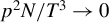 $p^2 N/T^3 \to 0$
. Among the IV approach, the DFIV estimator is more preferable. The GMM estimator requires that N grows at a rate faster than T; otherwise, the bias will not vanish asymptotically. In contrast, the DFIV estimator is free of any asymptotic bias without imposing any condition on the relative rate of growth for N and T.
$p^2 N/T^3 \to 0$
. Among the IV approach, the DFIV estimator is more preferable. The GMM estimator requires that N grows at a rate faster than T; otherwise, the bias will not vanish asymptotically. In contrast, the DFIV estimator is free of any asymptotic bias without imposing any condition on the relative rate of growth for N and T.
We investigate the finite-sample properties of these estimators through simulations in Section 4. Overall, the BCFE estimator has small bias and high precision but poor coverage probability, and it requires a sufficiently large T. In contrast, the IV estimators exhibit small bias and good coverage probability, but their finite sample distributions are more dispersed, and the GMM estimator requires a sufficiently large N.
Thus, we can conclude that if our concern is coverage probability or bias, then the DFIV estimator is recommended. On the other hand, if we care primarily about precision, then we recommend the BCFE estimator if T is not small compared to N and the GMM estimator when N is large and T is small.
3.8 Lag Selection
For the proposed estimators to be used in empirical applications, we need to choose the lag order of the approximated model, p. We consider the general-to-specific rule, which uses the t-statistic for the coefficient of the highest lag order in the model to test for the significance of the coefficients in each step.Footnote 12
Specifically, let $e_p$
be the
$e_p$
be the $p\times 1$
vector whose p-th element is
$p\times 1$
vector whose p-th element is $1$
and other elements are zero. Let
$1$
and other elements are zero. Let
 $$ \begin{align*} t_p( \hat{\alpha} (p)) = \sqrt{NT} e_p^{\prime }\hat{\alpha} (p) / \hat{v}_p, \end{align*} $$
where $\hat {\alpha } (p)$
and
$\hat {\alpha } (p)$
and $\hat {v}_p$
are estimators of
$\hat {v}_p$
are estimators of $\alpha (p)$
and
$\alpha (p)$
and $ v_p$
with
$ v_p$
with $\ell _p =e_p$
, respectively. The statistic
$\ell _p =e_p$
, respectively. The statistic $t_p (\hat {\alpha } (p)) $
is the t-test statistic for the null hypothesis
$t_p (\hat {\alpha } (p)) $
is the t-test statistic for the null hypothesis $\alpha _p =0$
based on estimator
$\alpha _p =0$
based on estimator $\hat {\alpha } (p)$
.
$\hat {\alpha } (p)$
.
We a priori set the maximum value of possible p, denoted $p_{\max }$
. Then, the general-to-specific procedure chooses
$p_{\max }$
. Then, the general-to-specific procedure chooses $\hat {p}$
as the maximum value of p such that
$\hat {p}$
as the maximum value of p such that $| t_p (\hat {\alpha } (p))|> z_{0.5\alpha } $
, where
$| t_p (\hat {\alpha } (p))|> z_{0.5\alpha } $
, where $z_{0.5\alpha }$
is the upper
$z_{0.5\alpha }$
is the upper $0.5\alpha $
quantile of the standard normal distribution, for
$0.5\alpha $
quantile of the standard normal distribution, for $p= 1, 2, \dots , p_{\max } $
.
$p= 1, 2, \dots , p_{\max } $
.
We make the following additional assumptions.
Assumption 6. (i) There exist constants $a_1>0$
and
$a_1>0$
and $d_1>1 $
such that
$d_1>1 $
such that $P(|\epsilon _{it}|>z) < \exp ( - (z/a_1)^{d_1})$
for sufficiently large z. (ii)
$P(|\epsilon _{it}|>z) < \exp ( - (z/a_1)^{d_1})$
for sufficiently large z. (ii) $w_{it} = y_{it} - \eta _i$
is strong mixing (as a sequence of t) with mixing coefficient
$w_{it} = y_{it} - \eta _i$
is strong mixing (as a sequence of t) with mixing coefficient $\alpha _i [k]$
satisfying
$\alpha _i [k]$
satisfying $\sup _i \alpha _i [k] < \exp (1- a_2 k^{d_2})$
for some
$\sup _i \alpha _i [k] < \exp (1- a_2 k^{d_2})$
for some $a_2>0$
ad
$a_2>0$
ad $d_2>0$
.
$d_2>0$
.
These assumptions allow us to use the high-dimensional central limit theorem and the Fuk–Nagaev inequality. Assumption 6 states that the tail of the distribution of the innovation term $\epsilon _{it}$
vanishes exponentially. This assumption guarantees that any finite moment of
$\epsilon _{it}$
vanishes exponentially. This assumption guarantees that any finite moment of $\epsilon _{it}$
exists and is stronger than the part of Assumption 1(i) related to
$\epsilon _{it}$
exists and is stronger than the part of Assumption 1(i) related to $\epsilon _{it}$
. It also implies that
$\epsilon _{it}$
. It also implies that $w_{it}$
has a distribution whose tail decays exponentially fast. Assumption 6(ii) imposes the mixing condition on
$w_{it}$
has a distribution whose tail decays exponentially fast. Assumption 6(ii) imposes the mixing condition on $w_{it}$
. Given that
$w_{it}$
. Given that $w_{it}$
is a linear process with i.i.d. innovations
$w_{it}$
is a linear process with i.i.d. innovations $\epsilon _{it}$
, this condition can be implied by some conditions on the distribution of
$\epsilon _{it}$
, this condition can be implied by some conditions on the distribution of $\epsilon _{it}$
and the properties of
$\epsilon _{it}$
and the properties of $\alpha _{k}, k = 1, \dots $
. However, such conditions tend to be complicated (see, e.g., Withers, Reference Withers1981) and we decide to state the assumptions in terms of
$\alpha _{k}, k = 1, \dots $
. However, such conditions tend to be complicated (see, e.g., Withers, Reference Withers1981) and we decide to state the assumptions in terms of $w_{it}$
directly.
$w_{it}$
directly.
The following theorem shows that the lag order selected by the general-to-specific procedure achieves an appropriate rate. The proof is in the Supplementary Material. We focus on the case in which $\hat \alpha (p) = \hat \alpha _{DF} (p)$
. Let
$\hat \alpha (p) = \hat \alpha _{DF} (p)$
. Let $\hat p$
be the lag order chosen by the general-to-specific procedure for the DFIV estimator.
$\hat p$
be the lag order chosen by the general-to-specific procedure for the DFIV estimator.
Theorem 10. Suppose that Assumptions 1 and 6 are satisfied. Let $p_{\min }$
be such that
$p_{\min }$
be such that $p_{\min } < p_{\max }$
,
$p_{\min } < p_{\max }$
, $p_{\max } - p_{\min } \to \infty $
, and
$p_{\max } - p_{\min } \to \infty $
, and $ \sqrt {N T p_{\max }}\sum _{k=p_{\min }+1}^{\infty } |\alpha _k| \to 0$
as
$ \sqrt {N T p_{\max }}\sum _{k=p_{\min }+1}^{\infty } |\alpha _k| \to 0$
as $N, T, p_{\min }, p_{\max } \to \infty $
. Assume that
$N, T, p_{\min }, p_{\max } \to \infty $
. Assume that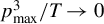 $p_{\max }^3 /T \to 0$
. Then, it holds that
$p_{\max }^3 /T \to 0$
. Then, it holds that $P( \hat p < p_{min}) \to 0$
as
$P( \hat p < p_{min}) \to 0$
as $N, T, p_{\min }, p_{\max } \to \infty $
.
$N, T, p_{\min }, p_{\max } \to \infty $
.
We set $p_{\max }$
such that the order of
$p_{\max }$
such that the order of $p_{\max }$
satisfies the conditions for the asymptotic normality of each estimator. In the simulation, we set
$p_{\max }$
satisfies the conditions for the asymptotic normality of each estimator. In the simulation, we set $p_{\max }=[12(T/100)^{1/4}] (=O(T^{1/4})),$
where
$p_{\max }=[12(T/100)^{1/4}] (=O(T^{1/4})),$
where $[x]$
is the integer part of x. In the case of least squares estimation, the order of p chosen by the sequential t tests is known to be the same as that of
$[x]$
is the integer part of x. In the case of least squares estimation, the order of p chosen by the sequential t tests is known to be the same as that of $p_{\max }$
(see Ng and Perron, Reference Ng and Perron1995; Lee et al., Reference Lee, Okui and Shintani2018).
$p_{\max }$
(see Ng and Perron, Reference Ng and Perron1995; Lee et al., Reference Lee, Okui and Shintani2018).
4 MONTE CARLO EXPERIMENTS
This section presents the results of our Monte Carlo simulations. We investigate the finite-sample performances of the IV estimators. For comparison, we also consider the BCFE estimator introduced in Lee et al. (Reference Lee, Okui and Shintani2018).
4.1 Design 1: Basic Comparisons
We generate samples from the ARMA(1,1) model of the following form:
 $$\begin{align*}y_{it}=\eta _{i}+\phi y_{i,t-1}+\epsilon _{it}+\theta \epsilon _{i,t-1}, \end{align*}$$
where $\phi =\{0.5,0.99\}$
,
$\phi =\{0.5,0.99\}$
, $\theta =0.4,$
and
$\theta =0.4,$
and $\eta _{i}\sim N(0,1)$
is independent across i,
$\eta _{i}\sim N(0,1)$
is independent across i, $\epsilon _{it}\sim N(0,1)$
is independent across i and t.Footnote
13
The individual effect
$\epsilon _{it}\sim N(0,1)$
is independent across i and t.Footnote
13
The individual effect $\eta _{i}$
and idiosyncratic error
$\eta _{i}$
and idiosyncratic error $\epsilon _{it}$
are also independently drawn. For each process,
$\epsilon _{it}$
are also independently drawn. For each process, $y_{i0}$
’s are generated from the (conditional) stationary distribution:
$y_{i0}$
’s are generated from the (conditional) stationary distribution:
 $$\begin{align*}y_{i0}|\eta _{i}\sim N\left( \frac{\eta _{i}}{1-\phi },\frac{1+\theta ^{2}+2\phi \theta }{1-\phi ^{2}}\right). \end{align*}$$
The pairs of N and T we consider are taken from the set $\{25,50,100\}$
. All the Monte Carlo simulation results are based on 10,000 replications.
$\{25,50,100\}$
. All the Monte Carlo simulation results are based on 10,000 replications.
We estimate the first AR coefficient $\alpha _{1}$
and the sum of the AR coefficients (SAR)
$\alpha _{1}$
and the sum of the AR coefficients (SAR) $ \sum _{k=1}^{\infty }\alpha _{k}$
using four alternative estimators: (i) the BCFE estimator
$ \sum _{k=1}^{\infty }\alpha _{k}$
using four alternative estimators: (i) the BCFE estimator $\hat {\alpha }_{BF}(p)$
; (ii) the AH estimator
$\hat {\alpha }_{BF}(p)$
; (ii) the AH estimator $\hat {\alpha }_{AH}(p)$
; (iii) the GMM estimator
$\hat {\alpha }_{AH}(p)$
; (iii) the GMM estimator $\hat {\alpha }_{G}(p)$
; and (iv) the DFIV estimator
$\hat {\alpha }_{G}(p)$
; and (iv) the DFIV estimator $\hat {\alpha }_{DF}(p)$
. When
$\hat {\alpha }_{DF}(p)$
. When $\phi =0.5$
(DGP1), true
$\phi =0.5$
(DGP1), true $\alpha _{1}$
and SAR are 0.9 and 0.643, respectively. When
$\alpha _{1}$
and SAR are 0.9 and 0.643, respectively. When $\phi =0.99$
(DGP2), the impulse response function is hump-shaped with true
$\phi =0.99$
(DGP2), the impulse response function is hump-shaped with true $\alpha _{1}$
being 1.390 and the process becomes highly persistent with the true SAR being near unity at 0.993. As illustrated in Figure 1, the autocorrelation function under DGP2 displays a markedly slow rate of decay, indicating extremely high persistence in the series.
$\alpha _{1}$
being 1.390 and the process becomes highly persistent with the true SAR being near unity at 0.993. As illustrated in Figure 1, the autocorrelation function under DGP2 displays a markedly slow rate of decay, indicating extremely high persistence in the series.
Autocorrelation function of DGP1 and DGP2.
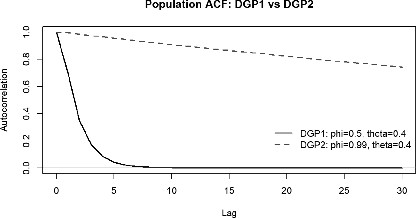
For the choice of lag length p in the approximated AR models, we consider both the fixed and automatically selected rules. For the fixed rule, we follow a conventional rule of thumb from the time-series literature and use $ p=[12(T/100)^{1/4}],$
where
$ p=[12(T/100)^{1/4}],$
where $[x]$
is the integer part of x. This fixed rule provides
$[x]$
is the integer part of x. This fixed rule provides $p=8$
,
$p=8$
, $10,$
and
$10,$
and $12$
for
$12$
for $T=25$
,
$T=25$
, $50,$
and
$50,$
and $100$
, respectively. The automatic lag selection rule corresponds to the general-to-specific procedure described in Section 3.8 with the maximum lag set at
$100$
, respectively. The automatic lag selection rule corresponds to the general-to-specific procedure described in Section 3.8 with the maximum lag set at $p_{\max }=[12(T/100)^{1/4}]$
and the significance level set at
$p_{\max }=[12(T/100)^{1/4}]$
and the significance level set at $\alpha =0.1$
. This implies that the automatic procedure always selects lags shorter than or equal to those using the fixed rule. At the same time, it should be noted that both the fixed and automatically selected rules satisfy the required conditions in the theoretical analysis.
$\alpha =0.1$
. This implies that the automatic procedure always selects lags shorter than or equal to those using the fixed rule. At the same time, it should be noted that both the fixed and automatically selected rules satisfy the required conditions in the theoretical analysis.
Table 1 shows the median bias, interquartile range (iqr), and coverage probability of an asymptotic 95% confidence interval when $N=100$
and
$N=100$
and $T=\{25,50,100\}$
.Footnote
14
The interquartile range (iqr) represents the difference between the 75th and 25th percentiles and is robust to outliers. The results clearly illustrate the bias properties of the estimators and are consistent with the theoretical predictions. For DGP1, the AH and the DFIV estimators have smaller bias than the GMM estimator. The bias of the GMM estimator is likely from the many-moment bias and higher-order bias not covered in our theoretical analysis. The bias of the DFIV estimator is the smallest among almost all the estimators for DGP1. The bias-correction procedure suggested in Lee et al. (Reference Lee, Okui and Shintani2018) reduces the bias of the FE estimator. The bias of the BCFE estimator is smaller than that of the GMM estimator for DGP1, and is comparable to that of the DFIV estimator under automatic lag selection for DGP2. All estimators have larger bias under DGP2, but it quickly decreases as p increases. Overall, the choice of lag selection method has little effect on the relative size of the median bias among estimators, whereas the selected lags from the automatic procedure clearly depend on the DGPs and estimators.
$T=\{25,50,100\}$
.Footnote
14
The interquartile range (iqr) represents the difference between the 75th and 25th percentiles and is robust to outliers. The results clearly illustrate the bias properties of the estimators and are consistent with the theoretical predictions. For DGP1, the AH and the DFIV estimators have smaller bias than the GMM estimator. The bias of the GMM estimator is likely from the many-moment bias and higher-order bias not covered in our theoretical analysis. The bias of the DFIV estimator is the smallest among almost all the estimators for DGP1. The bias-correction procedure suggested in Lee et al. (Reference Lee, Okui and Shintani2018) reduces the bias of the FE estimator. The bias of the BCFE estimator is smaller than that of the GMM estimator for DGP1, and is comparable to that of the DFIV estimator under automatic lag selection for DGP2. All estimators have larger bias under DGP2, but it quickly decreases as p increases. Overall, the choice of lag selection method has little effect on the relative size of the median bias among estimators, whereas the selected lags from the automatic procedure clearly depend on the DGPs and estimators.
Finite-sample performance of the estimators when N=100
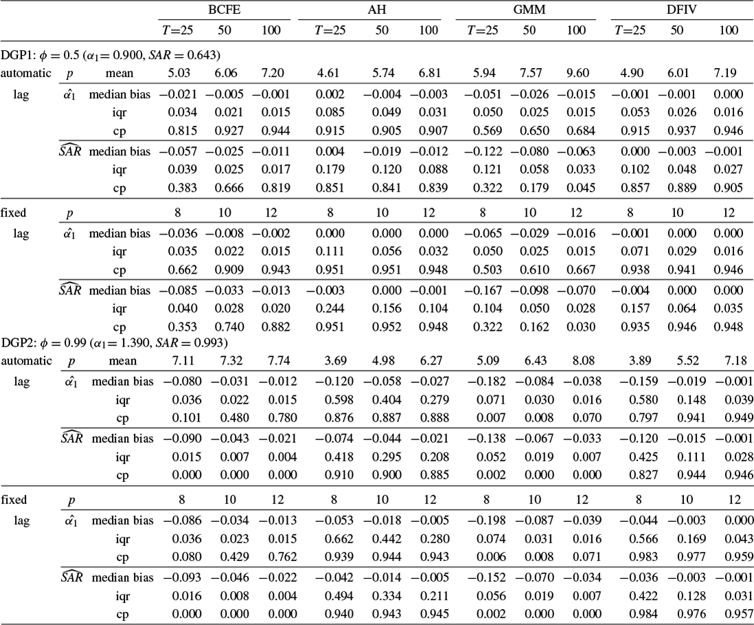
Note: Median of finite-sample bias (median bias), interquartile range (iqr), and coverage probability of 95% confidence interval (cp) of bias-corrected fixed effects (BCFE), Anderson–Hsiao (AH), GMM, and double filter IV (DFIV) estimators. Lag length is selected either by the sequential rule (automatic lag) with the maximum lag set at $[12(T/100)^{1/4}]$
or by the fixed rule (fixed lag) of
$[12(T/100)^{1/4}]$
or by the fixed rule (fixed lag) of $[12(T/100)^{1/4}]$
. 10,000 replications.
$[12(T/100)^{1/4}]$
. 10,000 replications.
The small bias property of the IV estimators is obtained at the cost of dispersion so that the interquartile ranges of the IV estimators are often very large. For both DGPs, the dispersion of BCFE is smaller than that of the AH, GMM, and the DFIV estimators. The dispersion measures of the GMM and the two other IV estimators, the AH and the DFIV, are comparable for DGP1 (with that of the AH being slightly larger), but the dispersion measures of the AH and the DFIV estimators are much larger than that of the GMM estimator for DGP2.
For the standard errors required in constructing the asymptotic confidence intervals of the GMM estimator $\hat {\alpha }_{G}(p)$
and the DFIV estimator
$\hat {\alpha }_{G}(p)$
and the DFIV estimator $\hat {\alpha }_{DF}(p)$
, we utilize the variance estimators
$\hat {\alpha }_{DF}(p)$
, we utilize the variance estimators $\hat {v}_{p,G}^{2}$
and
$\hat {v}_{p,G}^{2}$
and $\hat v_{p,DF}^2$
provided in Section 3.5. For the BCFE estimator
$\hat v_{p,DF}^2$
provided in Section 3.5. For the BCFE estimator $\hat \alpha _{BF}(p)$
, we use similarly defined variance estimator
$\hat \alpha _{BF}(p)$
, we use similarly defined variance estimator
 $$ \begin{align*} \hat{v}_{p,BF}^{2} =\left( \frac{1}{N(T-p)}\sum_{i=1}^{N}\sum_{t=p+1}^{T}( \tilde{y}_{it}-\tilde{x}_{it}(p)^{\prime }\hat{\alpha}_{BF}(p))^{2}\right) \ell _{p}^{\prime }(\hat{\Gamma}_{p}^{F})^{-1}\ell _{p}. \end{align*} $$
In terms of the coverage probability, the AH and DFIV estimators perform best for both DGPs. The performance of the BCFE estimator improves as T increases. However, its coverage probability of the confidence intervals for DGP2 is near zero. Finally, for either DGP1 or DGP2, the confidence intervals for the GMM estimator do not perform well because of the many-moment bias and higher-order bias.
4.2 Design 2: Decompositions
To evaluate the source of the finite-sample bias, we conduct an additional simulation exercise. As discussed in Section 3.6, the bias of each IV estimator is decomposed into the truncation bias and the fundamental bias. In the simulation, we can directly evaluate the relative contribution of each component because information about the true process is available. More specifically, the biases of the AH estimator, the GMM estimator, and the DFIV estimation in the simulation can be decomposed as
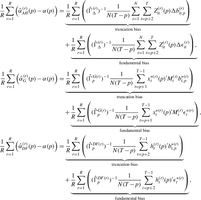 $$ \begin{align*} \frac{1}{R}\sum_{r=1}^{R}\left( \hat{\alpha}_{AH}^{(r)}(p)-\alpha (p)\right) &=\underbrace{\frac{1}{R}\sum_{r=1}^{R}\left( (\hat{\Gamma}_{\Delta}^{(r)}) ^{-1} \frac{1}{N(T-p)} \sum_{i=1}^{N} \sum_{t=p+2}^T Z_{it}^{(r)}(p)\Delta b_{it,p}^{(r)} \right) }_{\text{truncation bias}} \\ & \quad+\underbrace{\frac{ 1}{R}\sum_{r=1}^{R} \left( ( \hat{\Gamma}_{\Delta}^{(r)} ) ^{-1}\frac{1}{N(T-p)} \sum_{i=1}^{N} \sum_{t=p+2}^T Z_{it}^{(r)}(p)\Delta \epsilon_{it}^{(r)} \right), }_{\text{fundamental bias}} \\ \frac{1}{R}\sum_{r=1}^{R}\left( \hat{\alpha}_{G}^{(r)}(p)-\alpha (p)\right) &=\underbrace{\frac{1}{R}\sum_{r=1}^{R}\left( (\hat{\Gamma}_{p}^{G(r)})^{-1}\frac{1}{N(T-p)}\sum_{t=p+1}^{T-1}x_{t}^{\ast (r) }(p)^{\prime }M_{t}^{(r)}b_{t,p}^{\ast (r)}\right) }_{\text{truncation bias}} \\ & \quad+\underbrace{\frac{1}{R}\sum_{r=1}^{R}\left( (\hat{\Gamma}_{p}^{G(r)})^{-1}\frac{1}{N(T-p)} \sum_{t=p+1}^{T-1}x_{t}^{\ast (r)}(p)^{\prime }M_{t}^{(r)}\epsilon _{t}^{\ast (r)}\right) }_{\text{fundamental bias}}, \\ \frac{1}{R}\sum_{r=1}^{R}\left( \hat{\alpha}_{DF}^{(r)}(p)-\alpha (p)\right) &=\underbrace{\frac{1}{R}\sum_{r=1}^{R}\left( (\hat{\Gamma}_{p}^{DF(r)})^{-1}\frac{1}{N(T-p)}\sum_{t=p+2}^{T-1}h_{t}^{(r)}(p)^{\prime }b_{t,p}^{\ast (r) }\right) }_{\text{truncation bias}} \\ & \quad+\underbrace{\frac{ 1}{R}\sum_{r=1}^{R}\left( (\hat{\Gamma}_{p}^{DF(r)})^{-1}\frac{1}{N(T-p)} \sum_{t=p+2}^{T-1}h_{t}^{(r)}(p)^{\prime }\epsilon _{t}^{\ast (r)}\right) }_{\text{fundamental bias}}, \end{align*} $$
respectively, where the superscript r signifies the r-th simulated observation in R replications.
Table 2 provides such a decomposition of the finite-sample bias of the AH, GMM, and DFIV estimators when the data are generated from DGP1 and DGP2 with $N=\{25,50,100\}$
and
$N=\{25,50,100\}$
and $T=25$
. Since we expect the decreasing contribution of the truncation bias as lag length increases, we report the bias decomposition when the model is estimated using
$T=25$
. Since we expect the decreasing contribution of the truncation bias as lag length increases, we report the bias decomposition when the model is estimated using $p=\{2,4,8\}$
.Footnote
15
From the table, we observe that these two types of bias appear very different across the three estimators. For given N and p, the relative contribution of truncation bias in the total bias is the smallest for the GMM estimator and largest for the AH estimator. However, the GMM estimator exhibits a large fundamental bias when N is small. In contrast, the bias of the AH and the DFIV estimators comes solely from truncation bias. An important observation is that for the GMM estimator, there is a trade-off in the value of p such that as p increases, the truncation bias quickly vanishes but the fundamental bias increases. Unlike the GMM estimator, the fundamental biases of the AH and the DFIV estimators remain negligible, even when
$p=\{2,4,8\}$
.Footnote
15
From the table, we observe that these two types of bias appear very different across the three estimators. For given N and p, the relative contribution of truncation bias in the total bias is the smallest for the GMM estimator and largest for the AH estimator. However, the GMM estimator exhibits a large fundamental bias when N is small. In contrast, the bias of the AH and the DFIV estimators comes solely from truncation bias. An important observation is that for the GMM estimator, there is a trade-off in the value of p such that as p increases, the truncation bias quickly vanishes but the fundamental bias increases. Unlike the GMM estimator, the fundamental biases of the AH and the DFIV estimators remain negligible, even when $p=8$
.
$p=8$
.
Decomposition of the finite-sample bias of the estimators when $T=25$
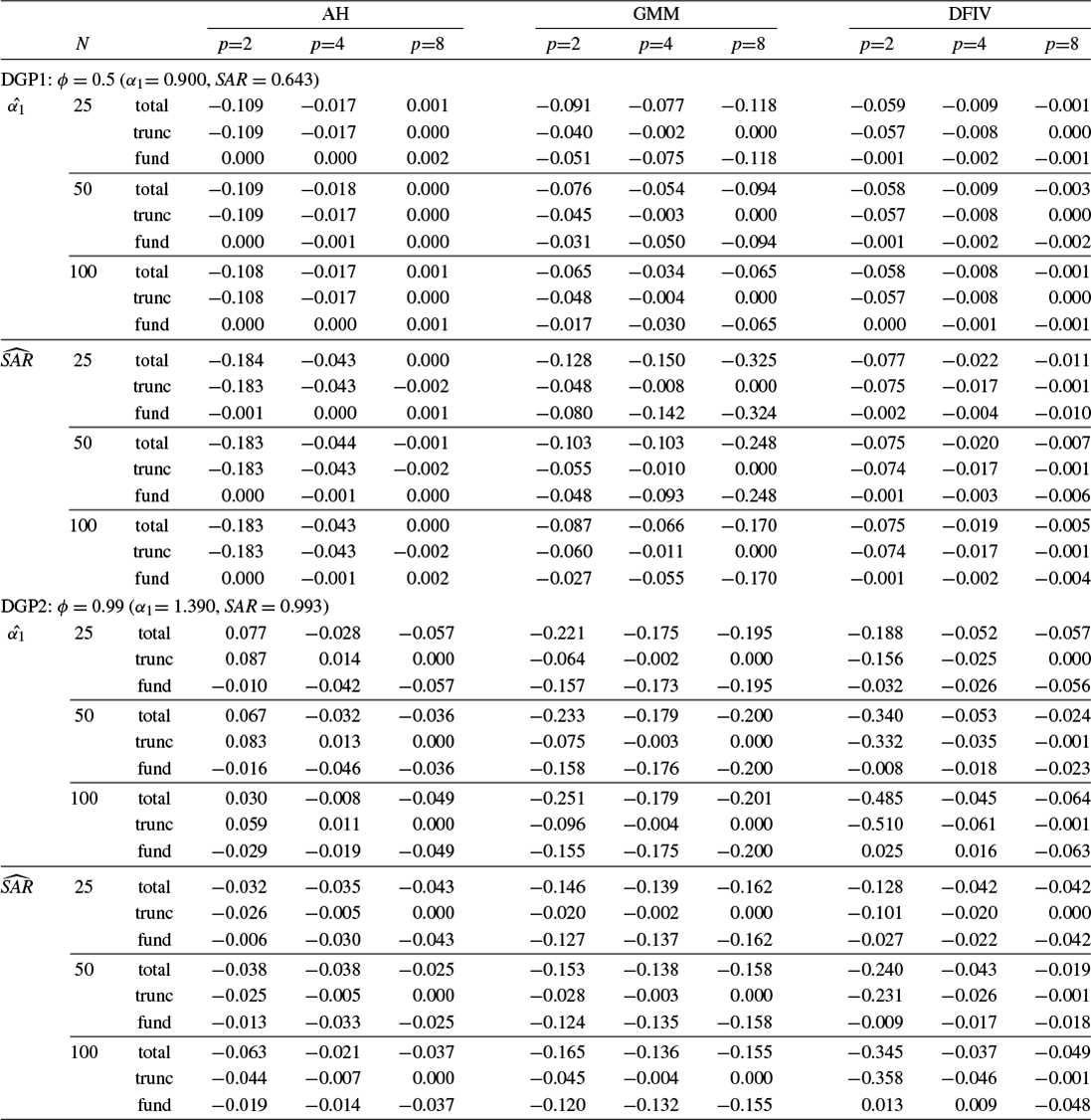
Note: Means of the components of the finite-sample bias of the Anderson–Hsiao (AH), GMM, and double filter IV (DFIV) estimators. The total finite-sample bias (total) is decomposed into truncation bias (trunc) and fundamental bias (fund). 10,000 replications.
Overall, the simulation results can be summarized as follows. If we care primarily about bias and dispersion, then we recommend the BCFE estimator. Alternatively, if our concern is bias and coverage probability, then the DFIV estimator is recommended.
4.3 Design 3: BCFE vs. DFIV Estimators
We now consider a design that enables a more in-depth comparison between the BCFE and DFIV estimators. Lee et al. (Reference Lee, Okui and Shintani2018) show that the BCFE estimator performs well when T is large. As discussed above, the DFIV estimator performs well when N is large relative to T. The theoretical results show that the DFIV estimator also remains effective as T increases. Thus, it is interesting to examine how the DFIV estimator compares to the BCFE estimator when T is large.
We use the same DGP setting as before, with $T = \{25, 50, 100\}$
and
$T = \{25, 50, 100\}$
and $N=25$
. We consider both homoskedastic and cluster-robust standard errors. For cluster-robust standard errors for the BCFE estimator, we use
$N=25$
. We consider both homoskedastic and cluster-robust standard errors. For cluster-robust standard errors for the BCFE estimator, we use
 $$ \begin{align*} \tilde{v}_{p,BF}^{2} \;=\; \ell_{p}'\,(\hat{\Gamma}_{p}^{F})^{-1} \left( \frac{1}{N(T-p)} \sum_{i=1}^{N}\sum_{t=p+1}^{T}\sum_{t'=p+1}^{T} \hat u_{it}^{\,*}\,\hat u_{it'}^{\,*}\; \tilde x_{it}(p)\,\tilde x_{it'}(p)^{\prime} \right) (\hat{\Gamma}_{p}^{F\prime})^{-1}\,\ell_{p}, \end{align*} $$
where
 $$ \begin{align*} \hat u_{it}^{\,*} \;=\; \tilde y_{it} - \tilde x_{it}(p)^{\prime}\hat{\alpha}_{BF}(p), \qquad \hat{\Gamma}_{p}^{F} \;=\; \frac{1}{N(T-p)}\sum_{t=p+1}^{T}\tilde x_{t}(p)^{\prime}\tilde x_{t}(p). \end{align*} $$
We estimate the models using the BCFE estimator and the DFIV estimator. The lag order is chosen by a general-to-specific rule starting from $p_{ ext{max}} = [12\,(T/100)^{1/4}]$
, based on the t-statistic computed with either homoskedastic or cluster-robust standard errors. Table 3 presents median bias, IQR, 95% confidence interval coverage, and mean lag order.
$p_{ ext{max}} = [12\,(T/100)^{1/4}]$
, based on the t-statistic computed with either homoskedastic or cluster-robust standard errors. Table 3 presents median bias, IQR, 95% confidence interval coverage, and mean lag order.
Finite-sample performance of the BCFE and DFIV estimators when N=25
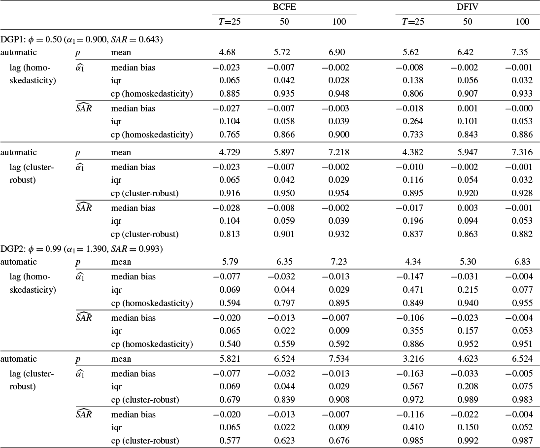
Note: Median of finite-sample bias (median bias), interquartile range (iqr), and coverage probability (cp) of the 95% confidence interval. Lag length is selected by the sequential general-to-specific rule with the maximum lag set at $[12(T/100)^{1/4}]$
. 10,000 replications.
$[12(T/100)^{1/4}]$
. 10,000 replications.
The bias of the DFIV estimator is smaller than that of the BCFE estimator under DGP1 in all cases. However, as T increases, the bias of the BCFE estimator decreases and becomes comparable to that of the DFIV estimator when $T=100$
. In contrast, under DGP2, the BCFE estimator has smaller bias than the DFIV estimator for
$T=100$
. In contrast, under DGP2, the BCFE estimator has smaller bias than the DFIV estimator for $T=25$
and
$T=25$
and $T=50$
. As T increases, the bias of the DFIV estimator decreases more rapidly and becomes smaller than that of the BCFE when
$T=50$
. As T increases, the bias of the DFIV estimator decreases more rapidly and becomes smaller than that of the BCFE when $T=100$
.
$T=100$
.
For both DGPs, the BCFE estimator has less dispersion than the DFIV estimator in all cases. DFIV’s dispersion is especially large under DGP2, while BCFE consistently shows low dispersion.
The BCFE estimator outperforms the DFIV estimator in terms of coverage probability under DGP1. However, under DGP2, coverage by the BCFE estimator is poor. Although coverage for the AR coefficient improves as T increases, the performance for the SAR component remains poor, even at larger values of T.
4.4 Design 4: GARCH Errors
Lastly, we consider a design with heteroskedastic errors. We have developed cluster-robust standard errors for the DFIV estimator, though our theoretical analyses assume homoskedasticity. Although asymptotic analyses with heteroskedastic errors are beyond the scope of this article, we use simulations to assess the performance of cluster-robust standard errors.
We retain the same ARMA(1,1) structure with individual effects but allow the shocks to follow a conditionally heteroskedastic GARCH(1,1) process:
 $$\begin{align*}y_{it}=\eta _{i}+\phi y_{i,t-1}+u_{it}+\theta u_{i,t-1}, \end{align*}$$
where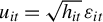 $u_{it}=\sqrt {h_{it}}\,\varepsilon _{it}$
with
$u_{it}=\sqrt {h_{it}}\,\varepsilon _{it}$
with $\varepsilon _{it}\sim \text {i.i.d. }N(0,1)$
, and
$\varepsilon _{it}\sim \text {i.i.d. }N(0,1)$
, and $h_{it}=\omega +\alpha _{garch}\,u_{i,t-1}^2+\beta _{garch}\,h_{i,t-1}$
with
$h_{it}=\omega +\alpha _{garch}\,u_{i,t-1}^2+\beta _{garch}\,h_{i,t-1}$
with $\omega $
chosen so that
$\omega $
chosen so that $E(h_{it})=1$
(thus
$E(h_{it})=1$
(thus $E(u_{it}^2)=1$
). We again consider DGP1 with
$E(u_{it}^2)=1$
). We again consider DGP1 with $(\phi ,\theta )=(0.5,0.4)$
and DGP2 with
$(\phi ,\theta )=(0.5,0.4)$
and DGP2 with $(\phi ,\theta )=(0.99,0.4)$
. We consider two GARCH specifications: a moderate case with
$(\phi ,\theta )=(0.99,0.4)$
. We consider two GARCH specifications: a moderate case with $(\alpha _{garch},\beta _{garch})=(0.1,0.8)$
and a near-IGARCH case with
$(\alpha _{garch},\beta _{garch})=(0.1,0.8)$
and a near-IGARCH case with $(\alpha _{garch},\beta _{garch})=(0.35,0.64)$
.
$(\alpha _{garch},\beta _{garch})=(0.35,0.64)$
.
To achieve stationarity within the data, we employ burn-in periods and discard initial observations. For the burn-in period, we set the first-period variance to its long-run average: $h_{i1}=E(h_{it})=\omega /(1-\alpha _{garch}-\beta _{garch})$
. We then discard 2,000 pre-sample observations in the moderate case and 3,000 in the near-IGARCH case.
$h_{i1}=E(h_{it})=\omega /(1-\alpha _{garch}-\beta _{garch})$
. We then discard 2,000 pre-sample observations in the moderate case and 3,000 in the near-IGARCH case.
For each DGP and GARCH specification, we set $T = \{25, 50, 100 \}$
with
$T = \{25, 50, 100 \}$
with $N=100$
. We estimate AR(p) models using the DFIV estimator. Results are shown for both homoskedastic and cluster-robust standard errors. The lag order is fixed by the rule
$N=100$
. We estimate AR(p) models using the DFIV estimator. Results are shown for both homoskedastic and cluster-robust standard errors. The lag order is fixed by the rule $p=[ 12\,(T/100)^{1/4}]$
. Table 4 reports median bias, IQR, and coverage probability of the nominal 95% confidence interval.
$p=[ 12\,(T/100)^{1/4}]$
. Table 4 reports median bias, IQR, and coverage probability of the nominal 95% confidence interval.
Finite-sample performance of the DFIV estimators under GARCH errors when N=100
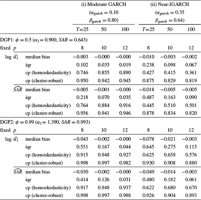
Note: Median of finite-sample bias (median bias), interquartile range (iqr), and coverage probability of 95% confidence interval based on two standard errors (cp) of double filter IV (DFIV) estimator. Lag length is selected by the fixed rule (fixed lag) of $[12(T/100)^{1/4}]$
. 10,000 replications.
$[12(T/100)^{1/4}]$
. 10,000 replications.
For DGP1, the coverage probability using cluster-robust standard errors is approximately 95% under the moderate GARCH case. However, it drops substantially under the near-IGARCH case. In contrast, the coverage probability with homoskedastic standard errors is already low for the moderate GARCH case. The deterioration further intensifies for the near-IGARCH case.
For DGP2, the coverage probability with cluster-robust standard errors remains high, while it is low with homoskedastic standard errors. Under the near-IGARCH, both estimators show improved coverage compared to DGP1.
5 CONCLUSION
In this article, we consider the IV estimation of a dynamic panel AR process of possibly infinite order in the presence of individual effects. We approximate and estimate the model by letting the order of the AR process of the fitted model increase with the sample size. In particular, we consider three IV estimators: the AH estimator, the GMM estimator, and the DFIV estimator. We study the asymptotic properties of the estimators and investigate their finite-sample properties in simulations. Among the three IV estimators, the DFIV estimator provides excellent performance in terms of the bias and coverage probability, but its finite-sample distribution is more dispersed when compared with the other estimators. The choice of estimators to be used should then depend on the relative magnitude of N and T and whether we care more about bias or overall precision. These findings are useful for making statistical inferences regarding quantities that are important in understanding the dynamic nature of an economic variable, such as long-run effects, without relying on strong assumptions.
We think that our approach can be extendable to broader frameworks. For instance, recent advances in dynamic panel estimation accommodate roots near unity and explosive roots (Phillips, Reference Phillips2018; Liu, Phillips, and Yu, Reference Liu, Phillips and Yu2023), thereby offering more robust inference methods. Additionally, developments in curved cross-sectional autoregression allow for general forms of cross-sectional dependence (Phillips and Jiang, Reference Phillips and Jiang2025a, Reference Phillips and Jiang2025b; Phillips, Reference Phillips2025) and are closely related to panel AR models. Extending our methodology to these more general settings is a promising avenue for future research.
APPENDIX
Throughout the appendix, $C\in (1,\infty )$
denotes a generic bounded constant, which does not depend on any index and whose actual value varies across occasions. Given a matrix A, we let
$C\in (1,\infty )$
denotes a generic bounded constant, which does not depend on any index and whose actual value varies across occasions. Given a matrix A, we let $||A||$
denote the Euclidean matrix norm defined by
$||A||$
denote the Euclidean matrix norm defined by $||A||^{2}=tr(A^{\prime }A)$
. Additionally, let
$||A||^{2}=tr(A^{\prime }A)$
. Additionally, let $||A||_{1}$
denote the Banach norm so that
$||A||_{1}$
denote the Banach norm so that $||A||_1 =\sup _{x\neq 0}\{||Ax||/||x||\}$
, using the Euclidean norm for the vector l,
$||A||_1 =\sup _{x\neq 0}\{||Ax||/||x||\}$
, using the Euclidean norm for the vector l, $||l||=(l^{\prime }l)^{1/2}$
. For any symmetric matrix A, we let
$||l||=(l^{\prime }l)^{1/2}$
. For any symmetric matrix A, we let $\lambda _{\min }(A)$
and
$\lambda _{\min }(A)$
and $\lambda _{\max }(A)$
be the minimum and the maximum eigenvalues of A, respectively. We note that
$\lambda _{\max }(A)$
be the minimum and the maximum eigenvalues of A, respectively. We note that $||A||_1 = \sqrt {\lambda _{\max } (A^{\prime }A)}$
. When A is symmetric and positive definite,
$||A||_1 = \sqrt {\lambda _{\max } (A^{\prime }A)}$
. When A is symmetric and positive definite, $||A||_{1}=\lambda _{\max }(A)$
. Define
$||A||_{1}=\lambda _{\max }(A)$
. Define $\gamma _k = E(w_{it} w_{i,t-k})$
. We let
$\gamma _k = E(w_{it} w_{i,t-k})$
. We let
 $$ \begin{align*} \bar{w}_{i,t,\tau} = \frac{1}{\tau-t +1} (w_{it}+ \dots + w_{i,\tau} ). \end{align*} $$
We also define $\bar {w}_{i,t,\tau } (p ) = (\bar {w}_{i,t,\tau }, \dots , \bar {w} _{i,t-p+1,\tau -p+1})^{\prime }$
,
$\bar {w}_{i,t,\tau } (p ) = (\bar {w}_{i,t,\tau }, \dots , \bar {w} _{i,t-p+1,\tau -p+1})^{\prime }$
, $\bar {w}_{t,\tau } =(\bar {w}_{1,t,\tau }, \dots , \bar {w}_{N, t, \tau })^{\prime }$
, and
$\bar {w}_{t,\tau } =(\bar {w}_{1,t,\tau }, \dots , \bar {w}_{N, t, \tau })^{\prime }$
, and $\bar {w}_{t,\tau } (p) = (\bar {w} _{t,\tau }, \dots , \bar {w}_{t-p+1,\tau -p+1} )$
. Similarly, define
$\bar {w}_{t,\tau } (p) = (\bar {w} _{t,\tau }, \dots , \bar {w}_{t-p+1,\tau -p+1} )$
. Similarly, define $\bar { \epsilon }_{i, t, \tau } = (\epsilon _{it} + \dots + \epsilon _{i,\tau })/(\tau -t+1)$
and
$\bar { \epsilon }_{i, t, \tau } = (\epsilon _{it} + \dots + \epsilon _{i,\tau })/(\tau -t+1)$
and $\bar {\epsilon }_{t,\tau } = (\bar {\epsilon } _{1, t, \tau } , \dots , \bar {\epsilon }_{N, t, \tau } )^{\prime }$
.
$\bar {\epsilon }_{t,\tau } = (\bar {\epsilon } _{1, t, \tau } , \dots , \bar {\epsilon }_{N, t, \tau } )^{\prime }$
.
The following inequalities will be used below: $||A||_{1}=\sqrt {\lambda _{\max }(A^{\prime }A)}\leq (tr(A^{\prime }A))^{1/2}=||A||$
.
$||A||_{1}=\sqrt {\lambda _{\max }(A^{\prime }A)}\leq (tr(A^{\prime }A))^{1/2}=||A||$
. $||AB||^{2}\leq ||A||_{1}^{2}||B||^{2}$
and
$||AB||^{2}\leq ||A||_{1}^{2}||B||^{2}$
and $||AB||^{2}\leq ||A||^{2}||B||_{1}^{2} $
(see Lewis and Reinsel, Reference Lewis and Reinsel1985; Wiener and Masani, Reference Wiener and Masani1958). For any conformable matrices A and D and any square matrix B,
$||AB||^{2}\leq ||A||^{2}||B||_{1}^{2} $
(see Lewis and Reinsel, Reference Lewis and Reinsel1985; Wiener and Masani, Reference Wiener and Masani1958). For any conformable matrices A and D and any square matrix B, $||A^{\prime }BD|| \le \| B \|_1 ||A|| \cdot ||D||$
.
$||A^{\prime }BD|| \le \| B \|_1 ||A|| \cdot ||D||$
.
We repeatedly use the result that there exists $C_{1}>0$
such that the minimum eigenvalue of
$C_{1}>0$
such that the minimum eigenvalue of $ \Gamma _{p}$
is greater than
$ \Gamma _{p}$
is greater than $C_{1}$
for any p and there exists
$C_{1}$
for any p and there exists $C_{2}< \infty $
such that the maximum eigenvalue of
$C_{2}< \infty $
such that the maximum eigenvalue of $\Gamma _{p}$
is smaller than
$\Gamma _{p}$
is smaller than $C_2$
for any p. This result holds under Assumption 1(iv) by Corollary 3.3 (i) and (ii) of Davies (Reference Davies1973).
$C_2$
for any p. This result holds under Assumption 1(iv) by Corollary 3.3 (i) and (ii) of Davies (Reference Davies1973).
A THE AH ESTIMATOR
We consider the AH type estimator:
 $$ \begin{align*} \hat{\alpha}_{AH}(p)=\left( \sum_{i=1}^{N} \sum_{t=p+2}^T Z_{it} (p)\Delta x_{it} (p)^{\prime }\right) ^{-1}\sum_{i=1}^{N} \sum_{t=p+3}^T Z_{it} (p)\Delta y_{it}. \end{align*} $$
Define
 $$ \begin{align*} \hat{\Gamma}_{\Delta } &=\frac{1}{N(T-p)}\sum_{i=1}^{N} \sum_{t=p+2}^T Z_{it} (p)\Delta x_{it} (p)^{\prime }, \\ U &=\frac{1}{N(T-p)}\sum_{i=1}^{N} \sum_{t=p+2}^T Z_{it} (p)\Delta u_{it,p}. \end{align*} $$
Then, we write
 $$ \begin{align*} \hat{\alpha}_{AH}(p)-\alpha (p)=\hat{\Gamma}_{\Delta }^{-1}U. \end{align*} $$
We also write
 $$ \begin{align*} U=U_{1}+U_{2}, \end{align*} $$
where
 $$ \begin{align*} U_{1} &=\frac{1}{N(T-p)}\sum_{i=1}^{N} \sum_{t=p+2}^T Z_{it} (p)\Delta b_{it,p}, \\ U_{2} &=\frac{1}{N(T-p)}\sum_{i=1}^{N} \sum_{t=p+2}^T Z_{it} (p)\Delta \epsilon _{it}. \end{align*} $$
We have the following lemmas. The proofs are in the Supplementary Material.
Lemma A.1. Suppose that Assumptions 1(i) and 1(iii) are satisfied. If $N\to \infty $
and
$N\to \infty $
and $T\to \infty $
, Then
$T\to \infty $
, Then
 $$ \begin{align*} || \hat{\Gamma}_{\Delta} - \Gamma_{\Delta} || = O_p \left( \frac{p}{\sqrt{N(T-p)}}\right). \end{align*} $$
Lemma A.2. Suppose that Assumptions 1 and 2 are satisfied. If $N\to \infty $
and
$N\to \infty $
and $T\to \infty $
, then
$T\to \infty $
, then
 $$ \begin{align*} || \hat{\Gamma}_{\Delta} - \Gamma_{\Delta} ||_1 = O_p \left( \frac{p}{\sqrt{N(T-p)}}\right). \end{align*} $$
Lemma A.3. Suppose that Assumptions 1 and 2 are satisfied. If $N\to \infty $
and
$N\to \infty $
and $T\to \infty $
with
$T\to \infty $
with $\lambda _p p / \sqrt {N(T-p)} \to 0$
, then
$\lambda _p p / \sqrt {N(T-p)} \to 0$
, then
 $$ \begin{align*} || \hat{\Gamma}_{\Delta}^{-1} - \Gamma_{\Delta}^{-1} ||_1 = O_p \left( \frac{\lambda_p^2 p }{\sqrt{N(T-p)}}\right). \end{align*} $$
Lemma A.4. Suppose that Assumptions 1 and 2 are satisfied. If $N\to \infty $
and
$N\to \infty $
and $T\to \infty $
with
$T\to \infty $
with $T^2/N \to 0$
, then
$T^2/N \to 0$
, then
 $$ \begin{align*} || \hat{\Gamma}_{\Delta}^{-1} ||_1 = O_p \left( \lambda_p + \frac{\lambda_p^2 p}{\sqrt{N(T-p)}}\right). \end{align*} $$
Proof. The result follows by observing that
 $$ \begin{align*} || \hat{\Gamma}_{\Delta}^{-1} ||_1 \le || \Gamma_{\Delta}^{-1} ||_1 + || \hat{\Gamma}_{\Delta}^{-1} - \hat{\Gamma}_{\Delta}^{-1} ||_1 = O_p \left( \lambda_p + \frac{\lambda_p^2 p}{\sqrt{N(T-p)}}\right) \end{align*} $$
Lemma A.5. Suppose that Assumptions 1 and 2 are satisfied. If $N, T, p \rightarrow \infty $
with
$N, T, p \rightarrow \infty $
with $p^{1/2}\sum _{k=p+1}^{\infty }|\alpha _{k}|\rightarrow 0$
, then
$p^{1/2}\sum _{k=p+1}^{\infty }|\alpha _{k}|\rightarrow 0$
, then
 $$ \begin{align*} ||U_{1}||=O_{p}\left( p^{1/2}\sum_{k=p+1}^{\infty }|\alpha _{k}|\right). \end{align*} $$
Lemma A.6. Suppose that Assumptions 1 and 2 are satisfied. If $N\to \infty $
and
$N\to \infty $
and $T\to \infty $
, then
$T\to \infty $
, then
 $$ \begin{align*} ||U_2 || = O_p \left(\frac{p}{\sqrt{N (T-p)}} \right). \end{align*} $$
Lemma A.7. Suppose that Assumptions 1 and 2 are satisfied. If $N\rightarrow \infty $
and
$N\rightarrow \infty $
and $T\rightarrow \infty $
with
$T\rightarrow \infty $
with $(T-p)\lambda _{p}^2 p/ N^2 = O(1)$
, then
$(T-p)\lambda _{p}^2 p/ N^2 = O(1)$
, then
 $$ \begin{align*} \sqrt{N(T-p)}\ell_{p}^{\prime }\Gamma _{\Delta }^{-1}U_{2}/v_{AH,p}\rightarrow _{d}N(0,1), \end{align*} $$
where
 $$ \begin{align*} v_{AH,p}^{2}=\frac{1}{(T-p)}E \left( \sum_{s = p+2}^T \sum_{s' = p+2}^T \Delta \epsilon _{i,s} \Delta \epsilon _{i,s'} \ell_p^{\prime }\Gamma _{\Delta}^{-1}Z_{is} (p)Z_{is'} (p)^{\prime }\Gamma _{\Delta }^{-1\prime }\ell_{p} \right). \end{align*} $$
A.1 Proof of Theorem 1
Proof. We have
 $$ \begin{align*} ||\hat{\alpha}_{AH} (p) - \alpha (p) || = || \hat{\Gamma}_{\Delta}^{-1} U || \le ||\hat{\Gamma}_{\Delta}^{-1}||_1 || U||. \end{align*} $$
Lemma A.4 gives that $||\hat {\Gamma }_{\Delta }^{-1}||_1 = O_p(\lambda _p + \lambda _p^2 p / \sqrt {N(T-p)})$
. Given
$||\hat {\Gamma }_{\Delta }^{-1}||_1 = O_p(\lambda _p + \lambda _p^2 p / \sqrt {N(T-p)})$
. Given
 $$ \begin{align*} ||U || \le ||U_1 || + ||U_2||. \end{align*} $$
Lemma A.5 gives that $||U_1 || = o_p(\sqrt {p} \sum _{k=p+1}^{\infty } |\alpha _k |)$
.
$||U_1 || = o_p(\sqrt {p} \sum _{k=p+1}^{\infty } |\alpha _k |)$
. $||U_2 || = o_p(p/\sqrt {N(T-p)})$
follows by Lemma A.6. Thus, when
$||U_2 || = o_p(p/\sqrt {N(T-p)})$
follows by Lemma A.6. Thus, when $\lambda _p \sqrt {p} \sum _{k=p+1}^{\infty } |\alpha _k | \to 0$
and
$\lambda _p \sqrt {p} \sum _{k=p+1}^{\infty } |\alpha _k | \to 0$
and $\lambda _p^2 p^2 / (N (T-p)) \to 0$
, we have
$\lambda _p^2 p^2 / (N (T-p)) \to 0$
, we have
 $$ \begin{align*} ||\hat{\alpha}_{AH} (p) - \alpha (p) || \to_p 0.\\[-31pt] \end{align*} $$
A.2 Proof of Theorem 2
Proof. We note that
 $$ \begin{align*} &\sqrt{N(T-p)} (\ell_{p}'\hat{\alpha}_{AH} (p) - \ell_{p}'\alpha (p) ) \\ &\quad= \sqrt{N(T-p)}\ell_{p}'\hat{\Gamma}_{\Delta}^{-1} U \\ &\quad= \sqrt{N(T-p)}\ell_{p}' \hat{\Gamma}_{\Delta}^{-1} U_1 + \sqrt{N(T-p)}\ell_{p}'\hat{\Gamma}_{\Delta}^{-1} U_2 \\ &\quad= \sqrt{N(T-p)}\ell_{p}' \hat{\Gamma}_{\Delta}^{-1} U_1 + \sqrt{N(T-p)}\ell_{p}' (\hat{\Gamma}_{\Delta}^{-1} - \Gamma_{\Delta}^{-1}) U_2 + \sqrt{N(T-p)}\ell_{p}'\Gamma_{\Delta}^{-1} U_2. \end{align*} $$
By Lemma A.7, we have
 $$ \begin{align*} \sqrt{N(T-p)}\ell_{p}'\Gamma_{\Delta}^{-1} U_2/v_{AH,p} \to_d N(0,1). \end{align*} $$
Next, we consider
 $$ \begin{align*} || \sqrt{N(T-p)}\ell_{p}' \hat{\Gamma}_{\Delta}^{-1} U_1|| \le || \ell_{p}||_1 ||\sqrt{N(T-p)} \hat{\Gamma}_{\Delta}^{-1} U_1|| \le || \ell_{p}||_1 || \hat{\Gamma}_{\Delta}^{-1}||_1 || \sqrt{N(T-p)} U_1||. \end{align*} $$
Now, we have $||\ell _{p}||_1 = \sqrt {\ell _{p}'\ell _{p}} \le C $
by the assumption (note that
$||\ell _{p}||_1 = \sqrt {\ell _{p}'\ell _{p}} \le C $
by the assumption (note that $\sqrt {\ell _{p}'\ell _{p}}$
is a scalar).
$\sqrt {\ell _{p}'\ell _{p}}$
is a scalar). $||\hat {\Gamma }_{\Delta }^{-1} ||_1 = O_p(\lambda _p + \lambda _p^2 p / \sqrt {N(T-p)})$
by Lemma A.4.
$||\hat {\Gamma }_{\Delta }^{-1} ||_1 = O_p(\lambda _p + \lambda _p^2 p / \sqrt {N(T-p)})$
by Lemma A.4. $||\sqrt {N(T-p)} U_1|| = O_p(\sqrt {N(T-p)p} \sum _{k=p+1}^{\infty } |\alpha _k |)$
by Lemma A.5. Therefore, when
$||\sqrt {N(T-p)} U_1|| = O_p(\sqrt {N(T-p)p} \sum _{k=p+1}^{\infty } |\alpha _k |)$
by Lemma A.5. Therefore, when $\lambda _p \sqrt {N(T-p)p} \sum _{k=p+1}^{\infty } |\alpha _k | \to 0 $
and
$\lambda _p \sqrt {N(T-p)p} \sum _{k=p+1}^{\infty } |\alpha _k | \to 0 $
and $\lambda _p^2 p^{3/2} \sum _{k=p+1}^{\infty } |\alpha _k | \to 0$
, we have
$\lambda _p^2 p^{3/2} \sum _{k=p+1}^{\infty } |\alpha _k | \to 0$
, we have $ || \sqrt {N}\ell _{p}' \hat {\Gamma }_{\Delta }^{-1} U_1|| = o_p(1)$
.
$ || \sqrt {N}\ell _{p}' \hat {\Gamma }_{\Delta }^{-1} U_1|| = o_p(1)$
.
Finally, we see that
 $$ \begin{align*} || \sqrt{N(T-p)}\ell_{p}' (\hat{\Gamma}_{\Delta}^{-1} - \Gamma_{\Delta}^{-1}) U_2|| \le || \ell_{p}||_1 || \hat{\Gamma}_{\Delta}^{-1} - \Gamma_{\Delta}^{-1}||_1 ||\sqrt{N(T-p)} U_2||. \end{align*} $$
We have $||\ell _{p}||_1 = \ell _{p}'\ell _{p} \le C $
.
$||\ell _{p}||_1 = \ell _{p}'\ell _{p} \le C $
. $||\hat {\Gamma }_{\Delta }^{-1} - \Gamma _{\Delta }^{-1} ||_1 = O_p( \lambda _p^2 p /\sqrt {N(T-p)})$
by Lemma A.3.
$||\hat {\Gamma }_{\Delta }^{-1} - \Gamma _{\Delta }^{-1} ||_1 = O_p( \lambda _p^2 p /\sqrt {N(T-p)})$
by Lemma A.3. $||\sqrt {N(T-p)} U_2|| = O_p(p)$
by Lemma A.6. Therefore, we have
$||\sqrt {N(T-p)} U_2|| = O_p(p)$
by Lemma A.6. Therefore, we have $ || \sqrt {N(T-p)}\ell _{p}' (\hat {\Gamma }_{\Delta }^{-1} - \Gamma _{\Delta }^{-1}) U_2|| = O_p ( \lambda _p^2 p^2 /\sqrt {N(T-p)})$
which is of order
$ || \sqrt {N(T-p)}\ell _{p}' (\hat {\Gamma }_{\Delta }^{-1} - \Gamma _{\Delta }^{-1}) U_2|| = O_p ( \lambda _p^2 p^2 /\sqrt {N(T-p)})$
which is of order $o_p(1)$
if
$o_p(1)$
if $\lambda _p^4 p^4 / (N(T-p)) \to 0$
.
$\lambda _p^4 p^4 / (N(T-p)) \to 0$
.
B LEMMAS USEFUL FOR THE GMM AND DFIV ESTIMATORS
This section presents several lemmas that are commonly employed in the derivation of the asymptotic properties of the GMM and DFIV estimators. Some are presented in Lee, Okui, and Shintani (Reference Lee, Okui and Shintani2017) which is the supplemental appendix to Lee et al. (Reference Lee, Okui and Shintani2018).
Lemma B.1 (Lee et al. (Reference Lee, Okui and Shintani2017, Lem. B.1)).
Suppose that Assumption 1 is satisfied. Then,
 $$ \begin{align*} || \bar{w}_{t,\tau} (p) ||^2 = O_p\left( \frac{Np}{\tau-t+1} \right) \text{ and } E || \bar{w}_{t,\tau} (p) ||^2 = O\left( \frac{Np}{\tau-t+1} \right). \end{align*} $$
Lemma B.2 (Lee et al. (Reference Lee, Okui and Shintani2017, Lem. B.2)).
Suppose that Assumption 1 is satisfied. If $N\to \infty $
,
$N\to \infty $
, $T\to \infty ,$
and
$T\to \infty ,$
and $p\to \infty $
with
$p\to \infty $
with $p/T \to 0$
, then
$p/T \to 0$
, then
 $$ \begin{align*} \left \Vert \frac{1}{N(T-p)} \sum_{t=p+1}^{T} w_{t-1} (p)^{\prime }w_{t-1} (p) - \Gamma_p \right \Vert = O_p \left( \frac{p}{\sqrt{NT}} \right). \end{align*} $$
Lemma B.3 (Lee et al. (Reference Lee, Okui and Shintani2018, Lem. A.1)).
Suppose that Assumption 1 is satisfied. Let $\hat {\Gamma }_p$
be an estimator of
$\hat {\Gamma }_p$
be an estimator of $\Gamma _p$
such that
$\Gamma _p$
such that $\left \Vert \hat {\Gamma }_p - \Gamma _p \right \Vert = O_p (\rho _{N,T,p}),$
where
$\left \Vert \hat {\Gamma }_p - \Gamma _p \right \Vert = O_p (\rho _{N,T,p}),$
where $\rho _{N,T,p} = o(1)$
as
$\rho _{N,T,p} = o(1)$
as $N\to \infty $
,
$N\to \infty $
, $T\to \infty ,$
and
$T\to \infty ,$
and $p\to \infty $
. Then, as
$p\to \infty $
. Then, as $N\to \infty $
,
$N\to \infty $
, $T\to \infty ,$
and
$T\to \infty ,$
and $p\to \infty $
, we have
$p\to \infty $
, we have
 $$ \begin{align*} ||\hat{\Gamma}_p - \Gamma_p ||_1 &= O_p\left( \rho_{N,T,p} \right), \\ ||(\hat{\Gamma}_p)^{-1} - \Gamma_p^{-1} ||_1 &= O_p\left(\rho_{N,T,p} \right), \\ \text{and } ||(\hat{\Gamma}_p)^{-1}||_1 &= O_p\left(1 \right). \end{align*} $$
Lemma B.4 (Lee et al. (Reference Lee, Okui and Shintani2017, Lem. B.3)).
Suppose that Assumption 1 is satisfied. If $N\to \infty $
,
$N\to \infty $
, $T\to \infty ,$
and
$T\to \infty ,$
and $p\to \infty $
with
$p\to \infty $
with $p^3/(NT) \to 0$
and
$p^3/(NT) \to 0$
and $p/T\to 0$
, then
$p/T\to 0$
, then
 $$ \begin{align*} \frac{1}{\sqrt{N(T-p)}} \ell_p^{\prime }\Gamma_p^{-1} \sum_{t=p+1}^T w_{t-1}(p)^{\prime }\epsilon_t / v_p \to_d N(0,1). \end{align*} $$
C THE GMM ESTIMATOR
This section presents several lemmas and the proofs of Theorems 3 and 4. The proofs of the lemmas are in the Supplementary Material. Note that variables with superscript “*” are transformed by the forward filter so that $b_{t,p}^* = \sqrt {(T-t)/(T-t+1)} (b_{t,p} - \sum _{\tau =t+1 }^{T}b_{\tau ,p}/(T-t))$
and
$b_{t,p}^* = \sqrt {(T-t)/(T-t+1)} (b_{t,p} - \sum _{\tau =t+1 }^{T}b_{\tau ,p}/(T-t))$
and $\epsilon _t^* = \sqrt {(T-t)/(T-t+1)} (\epsilon _{t} - \sum _{\tau =t+1 }^{T}\epsilon _{t}/(T-t)) $
. The estimation error of the GMM estimator can be decomposed as
$\epsilon _t^* = \sqrt {(T-t)/(T-t+1)} (\epsilon _{t} - \sum _{\tau =t+1 }^{T}\epsilon _{t}/(T-t)) $
. The estimation error of the GMM estimator can be decomposed as
 $$ \begin{align*} \hat{\alpha}(p) - \alpha (p) = (\hat{\Gamma}_p^G)^{-1} G_1 + (\hat{\Gamma}_p^G)^{-1} G_2, \end{align*} $$
where
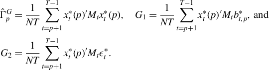 $$ \begin{align*} \hat{\Gamma}_p^G &= \frac{1}{NT} \sum_{t=p+1}^{T-1} x_t^* (p)^{\prime }M_t x_t^* (p), \quad G_1 = \frac{1}{NT}\sum_{t=p+1}^{T-1} x_t^* (p)^{\prime }M_t b_{t,p}^*, \text{ and }\\ G_2 &= \frac{1}{NT}\sum_{t=p+1}^{T-1} x_t^* (p)^{\prime }M_t \epsilon_{t}^*. \end{align*} $$
Note that we can write
 $$ \begin{align*} x_t ^* (p) = \sqrt{\frac{T-t}{T-t+1}} \left( w_{t-1} (p) - \bar{w}_{t,T-1} (p) \right). \end{align*} $$
Lemma C.1. Suppose that Assumptions 1 and 3 are satisfied. If $N\to \infty $
,
$N\to \infty $
, $T\to \infty ,$
and
$T\to \infty ,$
and $p\to \infty $
with
$p\to \infty $
with $p^2/T \to 0$
, then
$p^2/T \to 0$
, then
 $$ \begin{align*} ||\hat{\Gamma}_p^G - \Gamma_p || = O_p \left( \frac{p}{\sqrt{T}} \right). \end{align*} $$
Lemma C.2. Suppose that Assumption 1 is satisfied. If $N, T, p \rightarrow \infty $
with
$N, T, p \rightarrow \infty $
with $p^{1/2}\sum _{k=p+1}^{\infty }|\alpha _{k}|\rightarrow 0$
, then
$p^{1/2}\sum _{k=p+1}^{\infty }|\alpha _{k}|\rightarrow 0$
, then
 $$ \begin{align*} ||G_1 || = O_p \left(\sqrt{p} \sum_{k=p+1}^{\infty} |\alpha_k | \right) =o_p(1). \end{align*} $$
Suppose that Assumptions 1 and 3 are satisfied. If $N, T, p \rightarrow \infty $
with
$N, T, p \rightarrow \infty $
with $p^{1/2}\sum _{k=p+1}^{\infty }|\alpha _{k}|\rightarrow 0$
and
$p^{1/2}\sum _{k=p+1}^{\infty }|\alpha _{k}|\rightarrow 0$
and $p^2 /T \to 0$
, then
$p^2 /T \to 0$
, then
 $$ \begin{align*} || \ell_p' (\hat \Gamma_p^{G})^{-1} G_1 || = O_p \left( \sum_{k=p+1}^{\infty} |\alpha_k | \right). \end{align*} $$
Lemma C.3. Suppose that Assumptions 1, 3, and 4 are satisfied. If $N\to \infty $
,
$N\to \infty $
, $T\to \infty ,$
and
$T\to \infty ,$
and $p \to \infty $
with
$p \to \infty $
with $p \log T /T \to 0$
and
$p \log T /T \to 0$
and $T/N \to 0$
, then
$T/N \to 0$
, then
 $$ \begin{align*} ||G_2 || = O_p \left( \sqrt{\frac{p}{NT}} + \frac{\sqrt{p} \log T}{N} + \frac{\sqrt{p\log T}}{N^{3/4}\sqrt{T}} + \frac{p^{3/2}\sqrt{\log T}}{\sqrt{N}T}\right) = o_p(1). \end{align*} $$
Lemma C.4. Suppose that Assumptions 1, 3, and 4 are satisfied. If $N\to \infty $
,
$N\to \infty $
, $T\to \infty ,$
and
$T\to \infty ,$
and $p\to \infty $
with
$p\to \infty $
with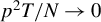 $p^2 T /N \to 0$
and
$p^2 T /N \to 0$
and $p^3 \log T /T \to 0$
, then
$p^3 \log T /T \to 0$
, then
 $$ \begin{align*} \sqrt{NT} \ell_p^{\prime }\Gamma_p^{-1} G_2/v_p \to_d N (0,1). \end{align*} $$
C.1 Proof of Theorem 3
Proof. We have
 $$ \begin{align*} ||\hat{\alpha}_G(p) - \alpha (p) || \le ||(\hat{\Gamma}_p^G)^{-1}||_1 || G_1|| + ||(\hat{\Gamma}_p^G)^{-1}||_1 || G_2||. \end{align*} $$
Lemmas B.3 and C.1 give that $||(\hat {\Gamma }_p^G)^{-1}||_1 = O_p(1)$
. Lemma C.2 gives that
$||(\hat {\Gamma }_p^G)^{-1}||_1 = O_p(1)$
. Lemma C.2 gives that $||G_1 || = o_p(1)$
when
$||G_1 || = o_p(1)$
when $p^{1/2} \sum _{k=p+1}^{\infty } \alpha _k \to 0$
and
$p^{1/2} \sum _{k=p+1}^{\infty } \alpha _k \to 0$
and $||G_2 || = o_p(1)$
follows by Lemma C.3.
$||G_2 || = o_p(1)$
follows by Lemma C.3.
C.2 Proof of Theorem 4
Proof. We note that
 $$ \begin{align*} &\sqrt{NT} (\ell_p'\hat{\alpha}_G (p) - \ell_p'\alpha (p) ) \\ &\quad= \sqrt{NT}\ell_p' (\hat{\Gamma}_p^G)^{-1} G_1 + \sqrt{NT}\ell_p' ((\hat{\Gamma}_p^G)^{-1} - \Gamma_p^{-1}) G_2 + \sqrt{NT}\ell_p'\Gamma_p^{-1} G_2. \end{align*} $$
Lemma C.2 provides that the first term is of order $o_p (1)$
by the assumption of the theorem. Lemma C.4 states that the third term is asymptotically standard normal.
$o_p (1)$
by the assumption of the theorem. Lemma C.4 states that the third term is asymptotically standard normal.
We consider the second term, and see that
 $$ \begin{align*} || \sqrt{NT}\ell_p' ((\hat{\Gamma}_p^G)^{-1} - \Gamma_p^{-1}) G_2|| \le || \ell_p||_1 || (\hat{\Gamma}_p^G)^{-1} - \Gamma_p^{-1}||_1 ||\sqrt{NT} G_2||. \end{align*} $$
We have $||\ell _p||_1 = \ell _p'\ell _p \le C $
.
$||\ell _p||_1 = \ell _p'\ell _p \le C $
. $||(\hat {\Gamma }_p^G)^{-1} - (\hat {\Gamma }_p^G)^{-1} ||_1 = O_p( p / T^{1/2})$
by Lemmas B.3 and C.1.
$||(\hat {\Gamma }_p^G)^{-1} - (\hat {\Gamma }_p^G)^{-1} ||_1 = O_p( p / T^{1/2})$
by Lemmas B.3 and C.1. $||\sqrt {NT} G_2|| = O_p(p^{1/2} + p^{1/2}T^{1/2}\log T /N^{1/2} + p^{1/2}(\log T)^{1/2} /N^{1/4} + p^{3/2} (\log T)^{1/2} / T^{1/2}) = O_p(p^{1/2})$
by Lemma C.3 and the condition that
$||\sqrt {NT} G_2|| = O_p(p^{1/2} + p^{1/2}T^{1/2}\log T /N^{1/2} + p^{1/2}(\log T)^{1/2} /N^{1/4} + p^{3/2} (\log T)^{1/2} / T^{1/2}) = O_p(p^{1/2})$
by Lemma C.3 and the condition that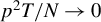 $p^2 T/N \to 0$
and
$p^2 T/N \to 0$
and $p^3 \log T /T \to 0$
. Therefore, we have
$p^3 \log T /T \to 0$
. Therefore, we have $ || \sqrt {NT}\ell _p' ((\hat {\Gamma }_p^G)^{-1} - \Gamma _p^{-1}) G_2|| = O_p ( p^{3/2}/T^{1/2})$
which is of order
$ || \sqrt {NT}\ell _p' ((\hat {\Gamma }_p^G)^{-1} - \Gamma _p^{-1}) G_2|| = O_p ( p^{3/2}/T^{1/2})$
which is of order $o_p(1)$
by the condition
$o_p(1)$
by the condition $ p^3 \log T /T \to 0$
.
$ p^3 \log T /T \to 0$
.
D THE DFIV ESTIMATOR
This section presents several lemmas and the proofs of Theorem 5 and 6. The proofs of the lemmas are in the Supplementary Material.
The estimation error of the DFIV estimator can be decomposed as
 $$ \begin{align*} \hat{\alpha}(p) - \alpha (p) = (\hat{\Gamma}_p^{DF})^{-1} D_1 + (\hat{\Gamma}_p^{DF})^{-1}D_2, \end{align*} $$
where
 $$ \begin{align*} \hat{\Gamma}_p^{DF} = \frac{1}{NT} \sum_{t=p+2}^{T-1} h_t (p)^{\prime }x_t^* (p), \quad D_1 = \frac{1}{NT}\sum_{t=p+2}^{T-1} h_t (p)^{\prime }b_{t,p}^*, \text{ and } D_2 = \frac{1}{NT}\sum_{t=p+2}^{T-1} h_t (p)^{\prime }\epsilon_{t}^*. \end{align*} $$
Note that we can write
 $$ \begin{align*} x_t ^* (p)& = \sqrt{\frac{T-t}{T-t+1}} \left( w_{t-1} (p) - \bar{w}_{t,T-1} (p) \right) \text{ and }\\ h_t (p) &= \sqrt{\frac{T-t}{T-t+1}} \left( w_{t-1} (p) - \bar{w}_{p,t-2} (p) \right). \end{align*} $$
Lemma D.1. Suppose that Assumption 1 is satisfied. If $N\to \infty $
,
$N\to \infty $
, $T\to \infty ,$
and
$T\to \infty ,$
and $p\to \infty $
with
$p\to \infty $
with $p^2/T \to 0$
, then
$p^2/T \to 0$
, then
 $$ \begin{align*} || \hat{\Gamma}_p^{DF} - \Gamma_p || = O_p \left( \frac{p}{\sqrt{T}} \right). \end{align*} $$
Lemma D.2. Suppose that Assumption 1 is satisfied. If $N, T, p \rightarrow \infty $
with
$N, T, p \rightarrow \infty $
with $p^{1/2}\sum _{k=p+1}^{\infty }|\alpha _{k}|\rightarrow 0$
, then
$p^{1/2}\sum _{k=p+1}^{\infty }|\alpha _{k}|\rightarrow 0$
, then
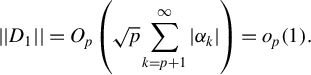 $$ \begin{align*} ||D_1 || = O_p \left(\sqrt{p} \sum_{k=p+1}^{\infty} |\alpha_k | \right) =o_p(1). \end{align*} $$
Suppose that Assumption 1 is satisfied. If $N, T, p \rightarrow \infty $
with
$N, T, p \rightarrow \infty $
with $p^{1/2}\sum _{k=p+1}^{\infty }|\alpha _{k}|\rightarrow 0$
and
$p^{1/2}\sum _{k=p+1}^{\infty }|\alpha _{k}|\rightarrow 0$
and $p^2/T \to 0$
, then
$p^2/T \to 0$
, then
 $$ \begin{align*} || \ell_p' (\hat \Gamma_p^{DF})^{-1} D_1 || = O_p \left( \sum_{k=p+1}^{\infty} |\alpha_k | \right). \end{align*} $$
Lemma D.3. Suppose that Assumption 1 is satisfied. If $N\to \infty $
,
$N\to \infty $
, $T\to \infty ,$
and
$T\to \infty ,$
and $p \to \infty $
with
$p \to \infty $
with $p/T \to 0$
, then
$p/T \to 0$
, then
 $$ \begin{align*} ||D_2 || = O_p \left( \sqrt{\frac{p}{NT}} \right) = o_p(1). \end{align*} $$
Lemma D.4. Suppose that Assumption 1 is satisfied. If $N\to \infty $
,
$N\to \infty $
, $T\to \infty ,$
and
$T\to \infty ,$
and $p\to \infty $
with
$p\to \infty $
with $p^3/(NT) \to 0$
and
$p^3/(NT) \to 0$
and $p^2 /T \to 0$
, then
$p^2 /T \to 0$
, then
 $$ \begin{align*} \sqrt{NT} \ell_p^{\prime }\Gamma_p^{-1} D_2/v_p \to_d N (0,1). \end{align*} $$
D.1 Proof of Theorem 5
Proof. We have
 $$ \begin{align*} ||\hat{\alpha}_{DF}(p) - \alpha (p) || = || ( \hat{\Gamma}_p^{DF})^{-1} (D_1 + D_2) || \le ||( \hat{\Gamma}_p^{DF})^{-1}||_1 || D_1|| + ||( \hat{\Gamma}_p^{DF})^{-1}||_1 || D_2||. \end{align*} $$
Lemmas B.3 and D.1 give that $||( \hat {\Gamma }_p^{DF})^{-1}||_1 = O_p(1)$
. Lemma D.2 gives that
$||( \hat {\Gamma }_p^{DF})^{-1}||_1 = O_p(1)$
. Lemma D.2 gives that $||D_1 || = o_p(1)$
and
$||D_1 || = o_p(1)$
and $||D_2 || = o_p(1)$
follows by Lemma D.3.
$||D_2 || = o_p(1)$
follows by Lemma D.3.
D.2 Proof of Theorem 6
Proof. We note that
 $$ \begin{align*} &\sqrt{NT} (\ell_p'\hat{\alpha}_{DF} (p) - \ell_p'\alpha (p) ) = \sqrt{NT}\ell_p' ( \hat{\Gamma}_p^{DF})^{-1} D_1 + \sqrt{NT}\ell_p'( \hat{\Gamma}_p^{DF})^{-1} D_2 \\ &\quad= \sqrt{NT}\ell_p' ( \hat{\Gamma}_p^{DF})^{-1} D_1 + \sqrt{NT}\ell_p' (( \hat{\Gamma}_p^{DF})^{-1} - \Gamma_p^{-1}) D_2 + \sqrt{NT}\ell_p'\Gamma_p^{-1} D_2. \end{align*} $$
By Lemma D.2, the first term is of order $o_p (1)$
under the assumption of the theorem. Lemma D.4 gives that the third term is asymptotically normal.
$o_p (1)$
under the assumption of the theorem. Lemma D.4 gives that the third term is asymptotically normal.
We now consider the second term and see that
 $$ \begin{align*} || \sqrt{NT}\ell_p' (( \hat{\Gamma}_p^{DF})^{-1} - \Gamma_p^{-1}) D_2|| \le || \ell_p||_1 || ( \hat{\Gamma}_p^{DF})^{-1} - \Gamma_p^{-1}||_1 ||\sqrt{NT} D_2||. \end{align*} $$
We have $||( \hat {\Gamma }_p^{DF})^{-1} - \Gamma _p^{-1} ||_1 = O_p( p / \sqrt {T})$
by Lemmas B.3 and D.1 and
$||( \hat {\Gamma }_p^{DF})^{-1} - \Gamma _p^{-1} ||_1 = O_p( p / \sqrt {T})$
by Lemmas B.3 and D.1 and $||\sqrt {NT} D_2|| =O_p(\sqrt {p})$
by Lemma D.3. These results imply that
$||\sqrt {NT} D_2|| =O_p(\sqrt {p})$
by Lemma D.3. These results imply that $ || \sqrt {NT}\ell _p' (( \hat {\Gamma }_p^{DF})^{-1} - \Gamma _p^{-1}) D_2|| = O_p ( p^{3/2}/\sqrt {T})$
which is of order
$ || \sqrt {NT}\ell _p' (( \hat {\Gamma }_p^{DF})^{-1} - \Gamma _p^{-1}) D_2|| = O_p ( p^{3/2}/\sqrt {T})$
which is of order $o_p(1)$
if
$o_p(1)$
if $ p^3 /T \to 0$
.
$ p^3 /T \to 0$
.
E THE DFIV ESTIMATOR WITH EXOGENOUS REGRESSORS
This section presents several lemmas and the proofs of Theorems 7 and 8. We redefine $w_{it}$
as
$w_{it}$
as $w_{it} =\sum _{k=0}^{\infty }\psi _{k}( (g_{i,t-k} - E(g_{i,t-k}))'\beta +\epsilon _{i,t-k})$
.
$w_{it} =\sum _{k=0}^{\infty }\psi _{k}( (g_{i,t-k} - E(g_{i,t-k}))'\beta +\epsilon _{i,t-k})$
.
Lemma E.1. Suppose that Assumptions 1 and 5 are satisfied. Then,
 $$ \begin{align*} || \bar{w}_{t,\tau} (p) ||^2 = O_p\left( \frac{Np}{\tau-t+1} \right) \text{ and } E || \bar{w}_{t,\tau} (p) ||^2 = O\left( \frac{Np}{\tau-t+1} \right). \end{align*} $$
Similarly,
 $$ \begin{align*} || \bar{g}_{t,\tau} ||^2 = O_p\left( \frac{N}{\tau-t+1} \right) \text{ and } E || \bar{g}_{t,\tau} ||^2 = O\left( \frac{N}{\tau-t+1} \right). \end{align*} $$
Let
 $$ \begin{align*} \Gamma_p^x = E \begin{pmatrix} w_{i,t-1} (p) w_{i,t-1} (p)' & w_{i,t-1} (p) g_{it}' \\ g_{it} w_{i,t-1} (p)' & g_{it} g_{it}' \end{pmatrix}. \end{align*} $$
Lemma E.2. Suppose that Assumptions 1 and 5 are satisfied. If $N\to \infty $
,
$N\to \infty $
, $T\to \infty ,$
and
$T\to \infty ,$
and $p\to \infty $
with
$p\to \infty $
with $p/T \to 0$
, then
$p/T \to 0$
, then
 $$ \begin{align*} \left \Vert \frac{1}{N(T-p)} \sum_{t=p+1}^{T} \begin{pmatrix} w_{t-1} (p)^{\prime }w_{t-1} (p) & w_{t-1} (p)^{\prime }g_t \\ g_t' w_{t-1} (p) & g_t'g_t \end{pmatrix}- \Gamma_p^x \right \Vert = O_p \left( \frac{p}{\sqrt{NT}} \right). \end{align*} $$
Lemma E.3. Suppose that Assumptions 1 and 5 are satisfied. Let $\hat {\Gamma }_p^x$
be an estimator of
$\hat {\Gamma }_p^x$
be an estimator of $\Gamma _p^x$
such that
$\Gamma _p^x$
such that $\left \Vert \hat { \Gamma }_p^x - \Gamma _p^x \right \Vert = O_p (\rho _{N,T,p}),$
where
$\left \Vert \hat { \Gamma }_p^x - \Gamma _p^x \right \Vert = O_p (\rho _{N,T,p}),$
where $\rho _{N,T,p} = o(1)$
as
$\rho _{N,T,p} = o(1)$
as $N\to \infty $
,
$N\to \infty $
, $T\to \infty ,$
and
$T\to \infty ,$
and $p\to \infty $
. Then, as
$p\to \infty $
. Then, as $N\to \infty $
,
$N\to \infty $
, $T\to \infty ,$
and
$T\to \infty ,$
and $p\to \infty $
, we have
$p\to \infty $
, we have
 $$ \begin{align} ||\hat{\Gamma}_p^x - \Gamma_p^x ||_1 &= O_p\left( \rho_{N,T,p} \right), \end{align} $$
 $$ \begin{align} ||(\hat{\Gamma}_p^x)^{-1} - (\Gamma_p^{x})^{-1} ||_1 &= O_p\left(\rho_{N,T,p} \right), \end{align} $$
 $$ \begin{align} \text{and } ||(\hat{\Gamma}_p^x)^{-1}||_1 &= O_p\left(1 \right). \end{align} $$
Lemma E.4. Suppose that Assumptions 1 and 5 are satisfied. If $N\to \infty $
,
$N\to \infty $
, $T\to \infty ,$
and
$T\to \infty ,$
and $p\to \infty $
with
$p\to \infty $
with $p^3/(NT) \to 0$
and
$p^3/(NT) \to 0$
and $p/T\to 0$
, then
$p/T\to 0$
, then
 $$ \begin{align*} \frac{1}{\sqrt{N(T-p)}} \ell_p^{\prime }(\Gamma_p^x)^{-1} \sum_{t=p+1}^T \begin{pmatrix} w_{t-1}(p)^{\prime } \\ g_t^{\prime} \end{pmatrix} \epsilon_t / v_p^x \to_d N(0,1), \end{align*} $$
where $v_p^x = \sigma ^2 \ell _p^{\prime } (\Gamma _p^x)^{-1} \ell _p$
.
$v_p^x = \sigma ^2 \ell _p^{\prime } (\Gamma _p^x)^{-1} \ell _p$
.
The estimation error of the DFIV estimator can be decomposed as
 $$ \begin{align*} \begin{pmatrix} \hat{\alpha}_{DF}(p) \\ \hat{\beta}_{DF} \end{pmatrix} - \begin{pmatrix} \alpha (p) \\ \beta \end{pmatrix} = (\hat{\Gamma}_p^{DFx})^{-1} D_1^x + (\hat{\Gamma}_p^{DFx})^{-1}D_2^x, \end{align*} $$
where
 $$ \begin{align*} &\hat{\Gamma}_p^{DFx} = \frac{1}{NT} \sum_{t=p+2}^{T-1} \begin{pmatrix} h_{t}(p)'x_{t}^{\ast }(p) & h_{t}(p)' g_{t}^{\ast } \\ g_{t}^{\ast \prime} x_{t}^{\ast }(p) & g_{t}^{\ast \prime} g_{t}^{\ast } \end{pmatrix}, \\ & D_1^x = \frac{1}{NT}\sum_{t=p+2}^{T-1}\begin{pmatrix} h_{t}(p)' \\ g_{t}^{\ast \prime} \end{pmatrix} b_{t,p}^*, \text{ and } D_2^x = \frac{1}{NT}\sum_{t=p+2}^{T-1}\begin{pmatrix} h_{t}(p) '\\ g_{t}^{\ast \prime} \end{pmatrix}\epsilon_{t}^*. \end{align*} $$
Note that we can write
 $$ \begin{align*} x_t ^* (p) &= \sqrt{\frac{T-t}{T-t+1}} \left( w_{t-1} (p) - \bar{w}_{t,T-1} (p) \right) \text{ and } \\h_t (p) &= \sqrt{\frac{T-t}{T-t+1}} \left( w_{t-1} (p) - \bar{w}_{p,t-2} (p) \right). \end{align*} $$
Lemma E.5. Suppose that Assumptions 1 and 5 are satisfied. If $N\to \infty $
,
$N\to \infty $
, $T\to \infty ,$
and
$T\to \infty ,$
and $p\to \infty $
with
$p\to \infty $
with $ p^2/T \to 0$
, then
$ p^2/T \to 0$
, then
 $$ \begin{align*} || \hat{\Gamma}_p^{DFx} - \Gamma_p^x || = O_p \left( \frac{p}{\sqrt{T}} \right). \end{align*} $$
Lemma E.6. Suppose that Assumptions 1 and 5 are satisfied. If $N\to \infty $
,
$N\to \infty $
, $T\to \infty ,$
and
$T\to \infty ,$
and $p\to \infty $
, then
$p\to \infty $
, then
 $$ \begin{align*} ||D_1^x || = O_p \left(\sqrt{p} \sum_{k=p+1}^{\infty} |\alpha_k | \right) =o_p(1). \end{align*} $$
Suppose that Assumptions 1 and 5 are satisfied. If $N\to \infty $
,
$N\to \infty $
, $T\to \infty ,$
and
$T\to \infty ,$
and $p\to \infty $
with
$p\to \infty $
with $p^2/T \to 0$
, then
$p^2/T \to 0$
, then
 $$ \begin{align*} || \ell_p' (\hat \Gamma_p^{DFx})^{-1} D_1^x || = O_p \left( \sum_{k=p+1}^{\infty} |\alpha_k | \right). \end{align*} $$
Lemma E.7. Suppose that Assumptions 1 and 5 are satisfied. If $N\to \infty $
,
$N\to \infty $
, $T\to \infty ,$
and
$T\to \infty ,$
and $p \to \infty $
with
$p \to \infty $
with $p/T \to 0$
, then
$p/T \to 0$
, then
 $$ \begin{align*} ||D_2^x || = O_p \left( \sqrt{\frac{p}{NT}} \right) = o_p(1). \end{align*} $$





F STANDARD ERRORS
F.1 Proof of Theorem 9
Proof. Let
 $$ \begin{align*} \hat B = \frac{1}{N(T-p)} \sum_{i=1}^N \sum_{t=p+2}^{T-1} \sum_{t' = p+2}^{T-1} \hat u_{it, D}^* \hat u_{it', D}^* h_{it}(p) h_{it'}(p). \end{align*} $$
We can write
 $$ \begin{align*} \tilde{v}_{p,DF}^{2} - v_{p}^2 &= \ell_p' (\hat{\Gamma}_{p}^{DF})^{-1} \hat B (\hat{\Gamma}_{p}^{DF\prime})^{-1} \ell_P - \ell_p' \Gamma_p^{-1} \Gamma_p \Gamma_p^{-1} \ell_p \\&= \ell_p' (\hat{\Gamma}_{p}^{DF})^{-1} (\hat B - \Gamma_p) \Gamma_p^{-1} \ell_p + \ell_p' ( (\hat{\Gamma}_{p}^{DF})^{-1} - \Gamma_p^{-1}) \Gamma_p \Gamma_p^{-1} \ell_p \\& \quad + \ell_p'(\hat{\Gamma}_{p}^{DF})^{-1} \hat B ( (\hat{\Gamma}_{p}^{DF})^{-1} - \Gamma_p^{-1})' \ell_p \\&\equiv V_1 + V_2 + V_3. \end{align*} $$
We show that $V_1$
,
$V_1$
, $V_2$
, and
$V_2$
, and $V_3$
are
$V_3$
are $o_p(1)$
.
$o_p(1)$
.
We first consider $V_1$
. Observe that
$V_1$
. Observe that
 $$ \begin{align*} ||V_1 || &\leq || \ell_p' (\hat{\Gamma}_{p}^{DF})^{-1} (\hat B - \Gamma_p) \Gamma_p^{-1} \ell_p || \leq ||\ell_p ||^2 || (\hat{\Gamma}_{p}^{DF})^{-1} ||_1 || (\hat B - \Gamma_p) ||_1 || \Gamma_p^{-1} ||_1 \\&= O_p\left( || (\hat B - \Gamma_p) ||_1\right) \end{align*} $$
by Lemmas B.3 and D.1. We now examine $\hat B- \Gamma _p$
. Because
$\hat B- \Gamma _p$
. Because $\hat u_{it', D}^* = - x_{it}^{\ast }(p)^{\prime }( \hat {\alpha }_{DF}(p) - \alpha (p)) + b_{it,p}^* + \epsilon _{it}^*$
, it follows that
$\hat u_{it', D}^* = - x_{it}^{\ast }(p)^{\prime }( \hat {\alpha }_{DF}(p) - \alpha (p)) + b_{it,p}^* + \epsilon _{it}^*$
, it follows that
 $$ \begin{align*} \hat B &= ( \hat{\alpha}_{DF}(p) - \alpha (p))' \frac{1}{N(T-p)} \sum_{i=1}^N \sum_{t=p+2}^{T-1} \sum_{t' = p+2}^{T-1} x_{it}^* (p) h_{it}(p) h_{it'}(p)' x_{it'}^{\ast \prime} (p) ( \hat{\alpha}_{DF}(p) - \alpha (p)) \\[1pt]&\quad - ( \hat{\alpha}_{DF}(p) - \alpha (p))' \frac{1}{N(T-p)} \sum_{i=1}^N \sum_{t=p+2}^{T-1} \sum_{t' = p+2}^{T-1} x_{it}^* (p) b_{it',p}^* h_{it}(p) h_{it'}(p)' \\[1pt]&\quad - ( \hat{\alpha}_{DF}(p) - \alpha (p))' \frac{1}{N(T-p)} \sum_{i=1}^N \sum_{t=p+2}^{T-1} \sum_{t' = p+2}^{T-1} x_{it}^* (p) \epsilon_{it'}^* h_{it}(p) h_{it'}(p)' \\[1pt]&\quad - \frac{1}{N(T-p)} \sum_{i=1}^N \sum_{t=p+2}^{T-1} \sum_{t' = p+2}^{T-1} b_{it,p}^* h_{it}(p) h_{it'}(p)' x_{it'}^{\ast \prime} (p) ( \hat{\alpha}_{DF}(p) - \alpha (p)) \\[1pt]&\quad + \frac{1}{N(T-p)} \sum_{i=1}^N \sum_{t=p+2}^{T-1} \sum_{t' = p+2}^{T-1} b_{it,p}^* b_{it',p}^* h_{it}(p) h_{it'}(p)' \\[1pt]&\quad + \frac{1}{N(T-p)} \sum_{i=1}^N \sum_{t=p+2}^{T-1} \sum_{t' = p+2}^{T-1} b_{it,p}^* \epsilon_{it'}^* h_{it}(p) h_{it'}(p)' \\[1pt]&\quad - \frac{1}{N(T-p)} \sum_{i=1}^N \sum_{t=p+2}^{T-1} \sum_{t' = p+2}^{T-1} \epsilon_{it}^* h_{it}(p) h_{it'}(p)' x_{it'}^{\ast \prime} (p) ( \hat{\alpha}_{DF}(p) - \alpha (p)) \\[1pt]&\quad + \frac{1}{N(T-p)} \sum_{i=1}^N \sum_{t=p+2}^{T-1} \sum_{t' = p+2}^{T-1} \epsilon_{it}^* b_{it',p}^* h_{it}(p) h_{it'}(p)'\\&\quad + \frac{1}{N(T-p)} \sum_{i=1}^N \sum_{t=p+2}^{T-1} \sum_{t' = p+2}^{T-1} \epsilon_{it}^* \epsilon_{it'}^* h_{it}(p) h_{it'}(p)'. \end{align*} $$
Each term can be analyzed by following the arguments in the proofs of Lemmas D.2 and D.3. First, we observe that
 $$ \begin{align*} & \left\Vert ( \hat{\alpha}_{DF}(p) - \alpha (p))' \frac{1}{N(T-p)} \sum_{i=1}^N \sum_{t=p+2}^{T-1} \sum_{t' = p+2}^{T-1} x_{it}^* (p) h_{it}(p) h_{it'}(p)' x_{it'}^{\ast \prime} (p) ( \hat{\alpha}_{DF}(p) - \alpha (p))\right\Vert \\ &\quad\leq || \hat{\alpha}_{DF}(p) - \alpha (p) ||^2 \frac{1}{N(T-p)} \sum_{i=1}^N \sum_{t=p+2}^{T-1} \sum_{t' = p+2}^{T-1} || x_{it}^* (p) ||_1 \cdot || h_{it}(p) ||_1 \cdot || h_{it'}(p) ||_1 \cdot ||x_{it'}^* \\ &(p) || \\ &\quad= O_p \left( \left( p \left(\sum_{k=p+1}^{\infty} | \alpha_k |\right)^2 + \frac{p}{NT} \right) \frac{N T^2 p^2}{NT} \right) = O_p \left( T p^3 \left(\sum_{k=p+1}^{\infty} | \alpha_k |\right)^2 + \frac{p^3}{N} \right). \end{align*} $$
Second,
 $$ \begin{align*} &\left\Vert ( \hat{\alpha}_{DF}(p) - \alpha (p))' \frac{1}{N(T-p)} \sum_{i=1}^N \sum_{t=p+2}^{T-1} \sum_{t' = p+2}^{T-1} x_{it}^* (p) b_{it',p}^* h_{it}(p) h_{it'}(p)' \right\Vert \\ &\quad\leq || \hat{\alpha}_{DF}(p) - \alpha (p) || \frac{1}{N(T-p)} \sum_{i=1}^N \sum_{t=p+2}^{T-1} || x_{it}^* (p) || \cdot || h_{it}(p) || \sum_{t' = p+2}^{T-1} || b_{it',p}^* h_{it'}(p)' || \\ &\quad= O_p \left( \left( \sqrt{p} \sum_{k=p+1}^{\infty} | \alpha_k |+ \sqrt{\frac{p}{NT}} \right) p T \sqrt{p} \sum_{k=p+1}^{\infty} | \alpha_k | \right) \\ &\quad= O_p \left( T p^2 \left( \sum_{k=p+1}^{\infty} | \alpha_k | \right)^2+ \frac{\sqrt{T} p^2 }{\sqrt{N}} \sum_{k=p+1}^{\infty} | \alpha_k | \right). \end{align*} $$
Third,
 $$ \begin{align*} &\left\Vert ( \hat{\alpha}_{DF}(p) - \alpha (p))' \frac{1}{N(T-p)} \sum_{i=1}^N \sum_{t=p+2}^{T-1} \sum_{t' = p+2}^{T-1} x_{it}^* (p) \epsilon_{it'}^* h_{it}(p) h_{it'}(p)' \right\Vert \\&\quad \leq || \hat{\alpha}_{DF}(p) - \alpha (p) || \frac{1}{N(T-p)} \sum_{i=1}^N \sum_{t=p+2}^{T-1} || x_{it}^* (p) || \cdot || h_{it}(p) || \cdot \left\Vert \sum_{t' = p+2}^{T-1} \epsilon_{it'}^* h_{it'}(p)' \right\Vert \\&\quad= O_p \left( \left( \sqrt{p} \sum_{k=p+1}^{\infty} | \alpha_k |+ \sqrt{\frac{p}{NT}} \right) p \sqrt{pT} \right) \\ &\quad= O_p \left( \left( \sqrt{T} p^2 \sum_{k=p+1}^{\infty} | \alpha_k |+ \frac{p^{5/2}}{\sqrt{N}} \right) \right). \end{align*} $$
The fourth term is the transpose of the second term and has the same order. The fifth term is
 $$ \begin{align*} & \left\Vert \frac{1}{N(T-p)} \sum_{i=1}^N \sum_{t=p+2}^{T-1} \sum_{t' = p+2}^{T-1} b_{it,p}^* b_{it',p}^* h_{it}(p) h_{it'}(p)' \right\Vert \\ &\quad\leq \frac{1}{N(T-p)} \sum_{i=1}^N \left\Vert \sum_{t=p+2}^{T-1} b_{it,p}^* h_{it}(p) \right\Vert^2 = O_p \left( T p \left(\sum_{k=p+1}^{\infty} | \alpha_k |\right)^2 \right). \end{align*} $$
The sixth term is
 $$ \begin{align*} & \left\Vert \frac{1}{N(T-p)} \sum_{i=1}^N \sum_{t=p+2}^{T-1} \sum_{t' = p+2}^{T-1}b_{it,p}^* \epsilon_{it'}^* h_{it}(p) h_{it'}(p)' \right\Vert \\ &\quad\leq \frac{1}{N(T-p)} \sum_{i=1}^N \left\Vert \sum_{t=p+2}^{T-1} \epsilon_{it}^* h_{it}(p) \right\Vert \cdot \left\Vert \sum_{t' = p+2}^{T-1} b_{it',p}^* h_{it'}(p)' \right\Vert \\ &\quad= O_p \left( \sqrt{p} \sum_{k=p+1}^{\infty} | \alpha_k | \sqrt{Tp} \right) = O_p \left( \sqrt{T} p \sum_{k=p+1}^{\infty} | \alpha_k | \right). \end{align*} $$
The seventh term is the transpose of the third term and has the same order. The eighth term is the transpose of the sixth term and has the same order. Lastly, we observe
 $$ \begin{align*} & \left\Vert \frac{1}{N(T-p)} \sum_{i=1}^N \sum_{t=p+2}^{T-1} \sum_{t' = p+2}^{T-1} \epsilon_{it}^* \epsilon_{it'}^* h_{it}(p) h_{it'}(p)' - \Gamma_p \right\Vert \\ &\quad\leq \left\Vert \frac{1}{N(T-p)} \sum_{i=1}^N \sum_{t=p+2}^{T-1} \sum_{t' = p+2}^{T-1} ( \epsilon_{it}^* \epsilon_{it'}^* h_{it}(p) h_{it'}(p)' - E (\epsilon_{it}^* \epsilon_{it'}^* h_{it}(p) h_{it'}(p)' ) ) \right\Vert \\ &\qquad+ \left\Vert \frac{1}{N(T-p)} \sum_{i=1}^N \sum_{t=p+2}^{T-1} \sum_{t' = p+2}^{T-1} E (\epsilon_{it}^* \epsilon_{it'}^* h_{it}(p) h_{it'}(p)' ) - \Gamma_p \right\Vert. \end{align*} $$
Now, we have
 $$ \begin{align*} & \left\Vert \frac{1}{N(T-p)} \sum_{i=1}^N \sum_{t=p+2}^{T-1} \sum_{t' = p+2}^{T-1} E (\epsilon_{it}^* \epsilon_{it'}^* h_{it}(p) h_{it'}(p)' ) - \Gamma_p \right\Vert \\ &\quad= \left\Vert \frac{T-p-1}{T-p} (\epsilon_{it}^* \epsilon_{it}^* h_{it}(p) h_{it'}(p)' ) - \Gamma_p \right\Vert \to 0. \end{align*} $$
It also holds that
 $$ \begin{align*} & E \left\Vert \frac{1}{N(T-p)} \sum_{i=1}^N \sum_{t=p+2}^{T-1} \sum_{t' = p+2}^{T-1} ( \epsilon_{it}^* \epsilon_{it'}^* h_{it}(p) h_{it'}(p)' - E (\epsilon_{it}^* \epsilon_{it'}^* h_{it}(p) h_{it'}(p)' ) ) \right\Vert^2 \\&\quad = \frac{1}{N(T-p)^2} E \left\Vert \sum_{t=p+2}^{T-1} \sum_{t' = p+2}^{T-1} ( \epsilon_{it}^* \epsilon_{it'}^* h_{it}(p) h_{it'}(p)' - E (\epsilon_{it}^* \epsilon_{it'}^* h_{it}(p) h_{it'}(p)' ) ) \right\Vert^2 \\ &\quad= O \left( \frac{p^2}{N} \right). \end{align*} $$
Thus, by the Chebyshev inequality,
 $$ \begin{align*} \left\Vert \frac{1}{N(T-p)} \sum_{i=1}^N \sum_{t=p+2}^{T-1} \sum_{t' = p+2}^{T-1} \epsilon_{it}^* \epsilon_{it'}^* h_{it}(p) h_{it'}(p)' - \Gamma_p \right\Vert =o_p(1). \end{align*} $$
To sum up, when $\sqrt {T}p^2 \sum _{k=p+1}^{\infty } |\alpha _k| \to 0$
and
$\sqrt {T}p^2 \sum _{k=p+1}^{\infty } |\alpha _k| \to 0$
and $p^5 /N \to 0$
,
$p^5 /N \to 0$
,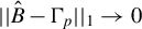 $ || \hat B - \Gamma _p ||_1 \to 0$
.
$ || \hat B - \Gamma _p ||_1 \to 0$
.
For $V_2$
, we have
$V_2$
, we have
 $$ \begin{align*} || V_2 || \leq || \ell_p' ( (\hat{\Gamma}_{p}^{DF})^{-1} - \Gamma_p^{-1}) \Gamma_p \Gamma_p^{-1} \ell_p ||_1 \leq || \ell_p ||^2 ||(\hat{\Gamma}_{p}^{DF})^{-1} - \Gamma_p^{-1} ||_1 = O_p \left( \frac{p}{\sqrt{T}}\right) \end{align*} $$
For $V_3$
, we have
$V_3$
, we have
 $$ \begin{align*} || V_3 || &\leq || \ell_p'(\hat{\Gamma}_{p}^{DF})^{-1} \hat B ( (\hat{\Gamma}_{p}^{DF})^{-1} - \Gamma_p^{-1})' \ell_p || \leq || \ell_p ||^2 || \hat{\Gamma}_{p}^{DF} ||_1 || \hat B ||_1 || (\hat{\Gamma}_{p}^{DF})^{-1}\\&\quad - \Gamma_p^{-1} ||_1 = O_p \left( \frac{p}{\sqrt{T}}\right) \end{align*} $$
COMPETING INTEREST STATEMENT
The authors declare that no competing interests exist.
FUNDING STATEMENT
R.O. acknowledges the financial support of the New Faculty Startup Fund and the Housing and Commercial Bank Economic Research Fund from the Institute of Economic Research at Seoul National University, and JSPS KAKENHI Grant numbers 22K20154 and 23K25501. M.S. acknowledges the financial support of JSPS KAKENHI Grant numbers 20H01482 and 24K00241.
SUPPLEMENTARY MATERIAL
Lee, Y.-J., Okui, R., & Shintani, M. (2026). Supplement to “Instrumental variables estimation for infinite order panel autoregressive processes,” Econometric Theory Supplementary Material. To view, please visit: https://doi.org/10.1017/S0266466626100401.






















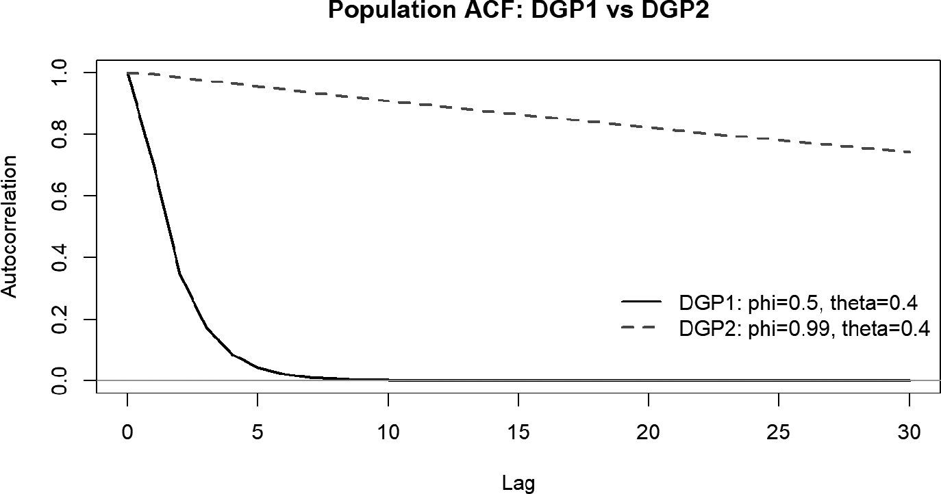
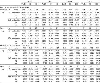
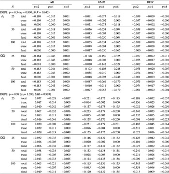

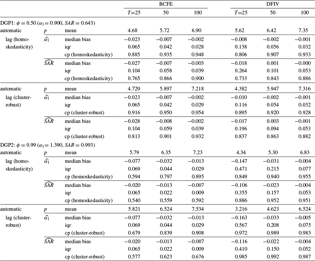
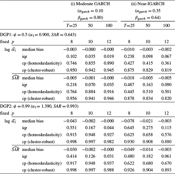


 Open access

