





1. Introduction
Prior to the discovery of the first planets orbiting other stars, it was generally accepted that other planetary systems would resemble the Solar system. With the discovery of the first exoplanets, that assumption was revealed to be wholly incorrect – with the first detected planets (the pulsar planets, Draugh, Poltergeist and Phobetor/PSR B1257 +12 b, c, and d; and the first ‘Hot Jupiter’ Dimidium/51 Pegasi b; Wolszczan & Frail Reference Wolszczan and Frail1992; Wolszczan Reference Wolszczan1994; Mayor & Queloz Reference Mayor and Queloz1995) proving utterly different to anything humanity had expected to find. Over the decades that followed, we discovered that the diversity of exoplanets was far greater than was ever anticipated based solely on our knowledge of the Solar system (e.g. Adams, Jackson, & Endl Reference Adams, Jackson and Endl2016; Zhu et al. Reference Zhu, Petrovich, Wu, Dong and Xie2018; Kunimoto & Matthews Reference Kunimoto and Matthews2020).Footnote a
The discovery and characterisation of exoplanets has now matured to the point where, in an age where more than 5 000 planets are known,Footnote b we can make meaningful observational tests of key questions in planet formation. One such question is: How common (or unusual) are systems like the Solar system? This mystery has tickled the imaginations of humans since they first looked up at the stars and wondered whether there was another Earth out there. For the first time, the current generation of scientists has the data to quantitatively address this question. This endeavour is of vital importance because the coming decades will see the advent of extremely large telescopes and flagship spacecraft missions designed to detect truly Earth-like planets in Earth-like orbits, and the search for life beyond the Solar system will begin in earnest (e.g. Horner & Jones Reference Horner and Jones2010; Fujii et al. Reference Fujii2018; Schwieterman et al. Reference Schwieterman2018; Harada et al. Reference Harada, Dressing, Kane and Ardestani2024a).
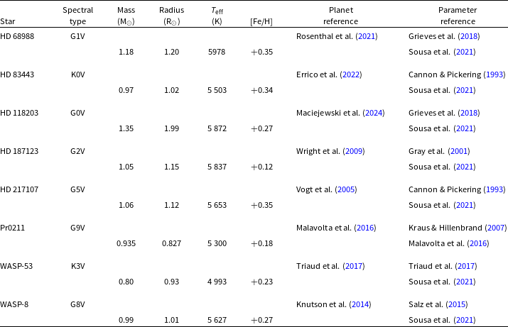
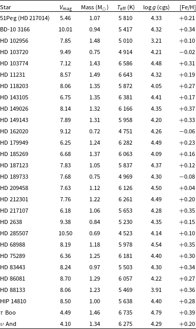
Stellar properties of the eight stars currently known to host a Hot Jupiter–Cold Jupiter pair.

One issue confounding our attempts to place the Solar system in the context of the ‘typical’ exoplanetary system is that the techniques used to find the vast majority of known exoplanets are strongly biased towards the discovery of planetary systems that are very different to our own (see e.g. Perryman Reference Perryman2018, and references therein). It is far easier to find massive planets orbiting close to their host stars than to find giant planets moving on decades-long orbits, like those seen in the Solar system. Similarly, detecting planets similar to the Solar system’s terrestrial worlds remains challenging – although as technology has improved over the years, such planets are now within our reach. Despite these challenges, however, a number of studies have been carried out attempting to bridge this gap and to determine how common are planets analogous to Jupiter (e.g. Wittenmyer et al. Reference Wittenmyer2016; Wittenmyer et al. Reference Wittenmyer2020). The California Legacy Survey (Rosenthal et al. Reference Rosenthal2021) and the Kepler Giant Planet Survey (Weiss et al. Reference Weiss2024) are currently carrying out ongoing programmes of radial velocity (RV) observations to search for such planets.
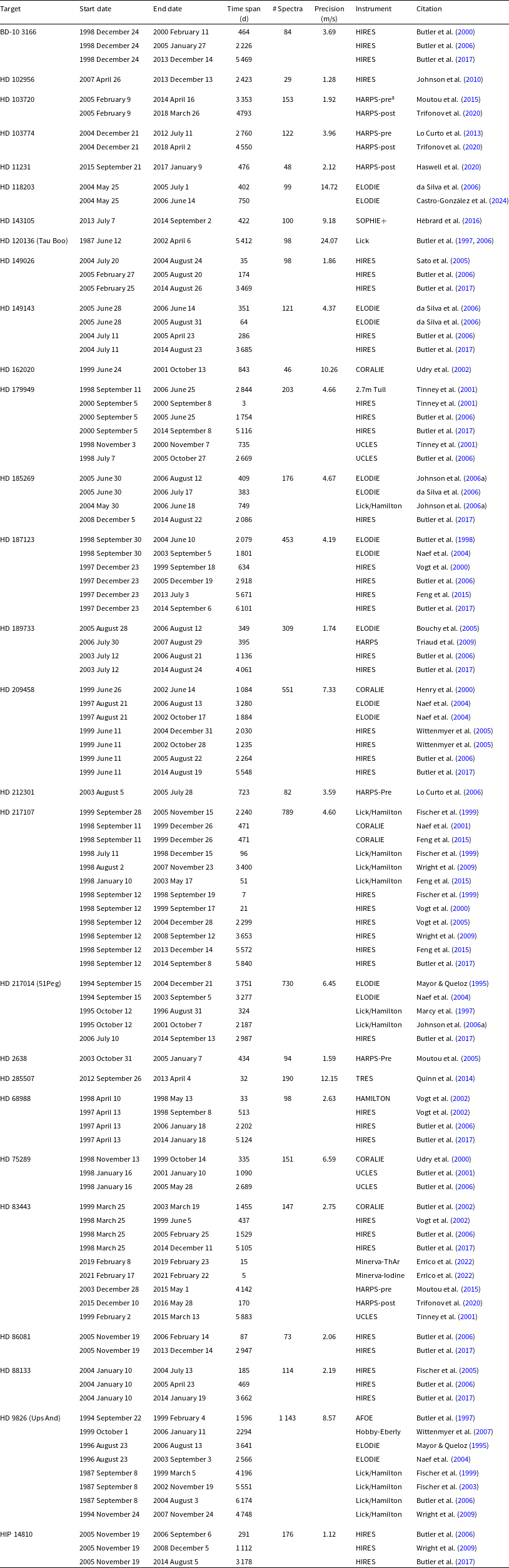
Details of the archival data for the planet host systems featured in this work. The start and end dates for each data set are provided, along with the span across which observations were made (the observational baseline). The number of spectra and median precision of that data (in m/s) are given for each star, along with details of the instruments used. A graphical representation of the time coverage, including gaps and overlaps, for each target is given in Figures 1 and 2.

aWe note here that HARPS underwent a fibre upgrade in 2015 (as described in Lo Curto et al. Reference Lo Curto2015), with the result that data from before and after the change needs to be considered as data from two separate instruments. To make these data explicit, we therefore denote observations made before the change as HARPS-pre, and data after the change as HARPS-post.
Earth-size planets appear to be extremely common (e.g. Wittenmyer et al. Reference Wittenmyer2011b; Dressing & Charbonneau Reference Dressing and Charbonneau2015; Zhu et al. Reference Zhu, Petrovich, Wu, Dong and Xie2018; Kunimoto & Matthews Reference Kunimoto and Matthews2020), and several tens of rocky planets are known to orbit in their host stars’ habitable zones (e.g. Gillon et al. Reference Gillon2017; Vanderburg et al. Reference Vanderburg2020; Gilbert et al. Reference Gilbert2023). However, these orbital properties are merely a necessary, but not sufficient, condition for a planet to be genuinely Earth-like (see e.g. Horner & Jones Reference Horner and Jones2010, Reference Horner and Jones2012; Waltham Reference Waltham2019; Airapetian et al. Reference Airapetian2020; Horner et al. Reference Horner2020a; Vervoort et al. Reference Vervoort, Horner, Kane, Kirtland Turner and Gilmore2022, and references therein). Occurrence rate studies suggest that there may be an embarrassment of riches in terms of potentially Earth-like planets, with some results indicating that frequency (eta-Earth) to be approaching unity (Bryson et al. Reference Bryson2021) – though large uncertainties remain due to incompleteness. Choosing the best candidates will be a critical task in the years to come.
The presence of ‘Jupiter analogues’: giant planets moving on low-eccentricity orbits beyond $\sim$
5 au (e.g. Wittenmyer et al. Reference Wittenmyer2011a; Zechmeister et al. Reference Zechmeister2013; Wittenmyer et al. Reference Wittenmyer2016; Bonomo et al. Reference Bonomo2023), is thought to be a factor influencing the habitability of inner rocky planets (see e.g. Wetherill Reference Wetherill1994, Reference Wetherill1995; Horner & Jones Reference Horner and Jones2008, Reference Horner and Jones2009; Horner, Jones, & Chambers Reference Horner, Jones and Chambers2010; Grazier Reference Grazier2016; Raymond & Izidoro Reference Raymond and Izidoro2017; Vervoort et al. Reference Vervoort, Horner, Kane, Kirtland Turner and Gilmore2022). The low eccentricities of such giant planets could indicate a relatively benign dynamical history for the system, enhancing the probability of an interior rocky planet remaining on a long-term stable, near-circular orbit like our Earth. Distant giant planets with high-eccentricity orbits are also of interest; cold giants that remain beyond the snow line are expected to have retained low-eccentricity orbits, unless perturbed by interactions with other planets. Such planet-planet scattering can result in ejections, or one planet being hurled into a highly elliptical orbit, and would also significantly destabilise the small bodies in the system – leading to periods of extreme impact rates on any terrestrial planet analogues (e.g. Gomes et al. Reference Gomes, Levison, Tsiganis and Morbidelli2005; Levison et al. Reference Levison, Morbidelli, Tsiganis, Nesvorný and Gomes2011; Nesvorný Reference Nesvorný2018), but potentially also delivering a wealth of volatile material to those planets (e.g. Owen & Bar-Nun Reference Owen and Bar-Nun1995; Morbidelli et al. Reference Morbidelli2000; Horner et al. Reference Horner, Mousis, Petit and Jones2009; O’Brien et al. Reference O’Brien, Walsh, Morbidelli, Raymond and Mandell2014; Raymond & Izidoro Reference Raymond and Izidoro2017). These dynamical fingerprints are important evidence for determining the frequency of various outcomes of post-formation processes.
$\sim$
5 au (e.g. Wittenmyer et al. Reference Wittenmyer2011a; Zechmeister et al. Reference Zechmeister2013; Wittenmyer et al. Reference Wittenmyer2016; Bonomo et al. Reference Bonomo2023), is thought to be a factor influencing the habitability of inner rocky planets (see e.g. Wetherill Reference Wetherill1994, Reference Wetherill1995; Horner & Jones Reference Horner and Jones2008, Reference Horner and Jones2009; Horner, Jones, & Chambers Reference Horner, Jones and Chambers2010; Grazier Reference Grazier2016; Raymond & Izidoro Reference Raymond and Izidoro2017; Vervoort et al. Reference Vervoort, Horner, Kane, Kirtland Turner and Gilmore2022). The low eccentricities of such giant planets could indicate a relatively benign dynamical history for the system, enhancing the probability of an interior rocky planet remaining on a long-term stable, near-circular orbit like our Earth. Distant giant planets with high-eccentricity orbits are also of interest; cold giants that remain beyond the snow line are expected to have retained low-eccentricity orbits, unless perturbed by interactions with other planets. Such planet-planet scattering can result in ejections, or one planet being hurled into a highly elliptical orbit, and would also significantly destabilise the small bodies in the system – leading to periods of extreme impact rates on any terrestrial planet analogues (e.g. Gomes et al. Reference Gomes, Levison, Tsiganis and Morbidelli2005; Levison et al. Reference Levison, Morbidelli, Tsiganis, Nesvorný and Gomes2011; Nesvorný Reference Nesvorný2018), but potentially also delivering a wealth of volatile material to those planets (e.g. Owen & Bar-Nun Reference Owen and Bar-Nun1995; Morbidelli et al. Reference Morbidelli2000; Horner et al. Reference Horner, Mousis, Petit and Jones2009; O’Brien et al. Reference O’Brien, Walsh, Morbidelli, Raymond and Mandell2014; Raymond & Izidoro Reference Raymond and Izidoro2017). These dynamical fingerprints are important evidence for determining the frequency of various outcomes of post-formation processes.
Systems containing highly eccentric cold giant planets are of particular interest as they tell an intriguing story of their misspent youth. Errico et al. (Reference Errico2022) reported the discovery of a giant planet with a 22-yr orbital period and an eccentricity of $e=0.76$
in the HD 83443 system, which was already known to host a Hot Jupiter (Butler et al. Reference Butler2002). This system configuration, with a Hot Jupiter and an eccentric distant Cold Jupiter, is quite rare, with the HD 83443 system being only the eighth such system detected.Footnote
c
The eccentric outer planet is thought to have originated from a dynamical event which scattered the Hot Jupiter inward while sending the outer planet into its highly elliptical orbit. The discovery naturally raises the question: How common is this outcome?
$e=0.76$
in the HD 83443 system, which was already known to host a Hot Jupiter (Butler et al. Reference Butler2002). This system configuration, with a Hot Jupiter and an eccentric distant Cold Jupiter, is quite rare, with the HD 83443 system being only the eighth such system detected.Footnote
c
The eccentric outer planet is thought to have originated from a dynamical event which scattered the Hot Jupiter inward while sending the outer planet into its highly elliptical orbit. The discovery naturally raises the question: How common is this outcome?
In this work, we examine all known Hot Jupiter systems which have publicly available RV data and ask how many ‘HD 83443-like’ systems with an outer cold giant planet (‘acquaintances of Hot Jupiters’) could be lurking undetected. We model how future observations will impact the likelihood of finding cold giant planets of different masses at a variety of distances and examine the roles of observation cadence and instrumental precision on these results. Section 2 describes the extant observational data used to perform the simulations that are described in Section 3. Section 4 gives our results for 28 Hot Jupiter systems: both the current state of detectability for such Hot Jupiter–Cold Jupiter systems, and the degree to which such planets would be detected under various observing scenarios. Finally in Section 5 we give our conclusions.
2. Observations
We selected the Hot Jupiters from the NASA Exoplanet Archive with the following criteria: orbital period $\lt$
10 d; semi-major axis
$\lt$
10 d; semi-major axis $\lt$
0.1 au; and mass
$\lt$
0.1 au; and mass $\gt$
0.3 Jupiter mass (
$\gt$
0.3 Jupiter mass ( $M_\mathrm{Jup}$
). Because we are interested in RV sensitivity to distant cold giant planets, we filtered our sample to include only those 37 Hot Jupiters that were discovered using that method. Whilst hundreds of Hot Jupiters are known from transit surveys, including them here would introduce a severe bias: such planets tend to be confirmed with only a short span of radial velocities, and hence their data would be useless in constraining the presence of long-period planets. We then obtained all publicly-available data from the Data & Analysis Center for Exoplanets (DACE database), a web platform at the University of Geneva dedicated to extrasolar planets data visualisation, exchange, and analysis)Footnote
d
and from the HARPS RVBank (Trifonov et al. Reference Trifonov2020) for the planets in our sample.
$M_\mathrm{Jup}$
). Because we are interested in RV sensitivity to distant cold giant planets, we filtered our sample to include only those 37 Hot Jupiters that were discovered using that method. Whilst hundreds of Hot Jupiters are known from transit surveys, including them here would introduce a severe bias: such planets tend to be confirmed with only a short span of radial velocities, and hence their data would be useless in constraining the presence of long-period planets. We then obtained all publicly-available data from the Data & Analysis Center for Exoplanets (DACE database), a web platform at the University of Geneva dedicated to extrasolar planets data visualisation, exchange, and analysis)Footnote
d
and from the HARPS RVBank (Trifonov et al. Reference Trifonov2020) for the planets in our sample.
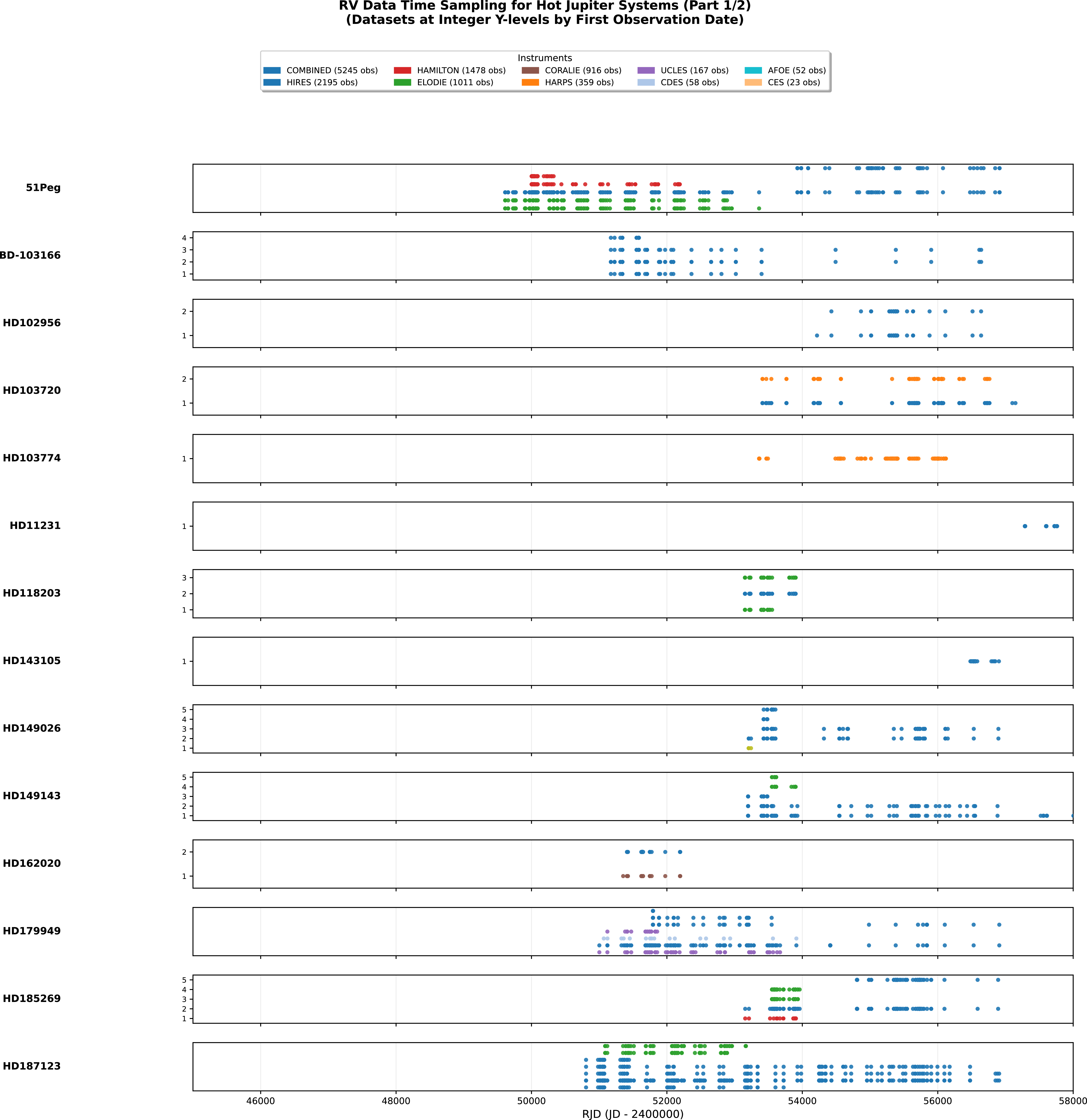
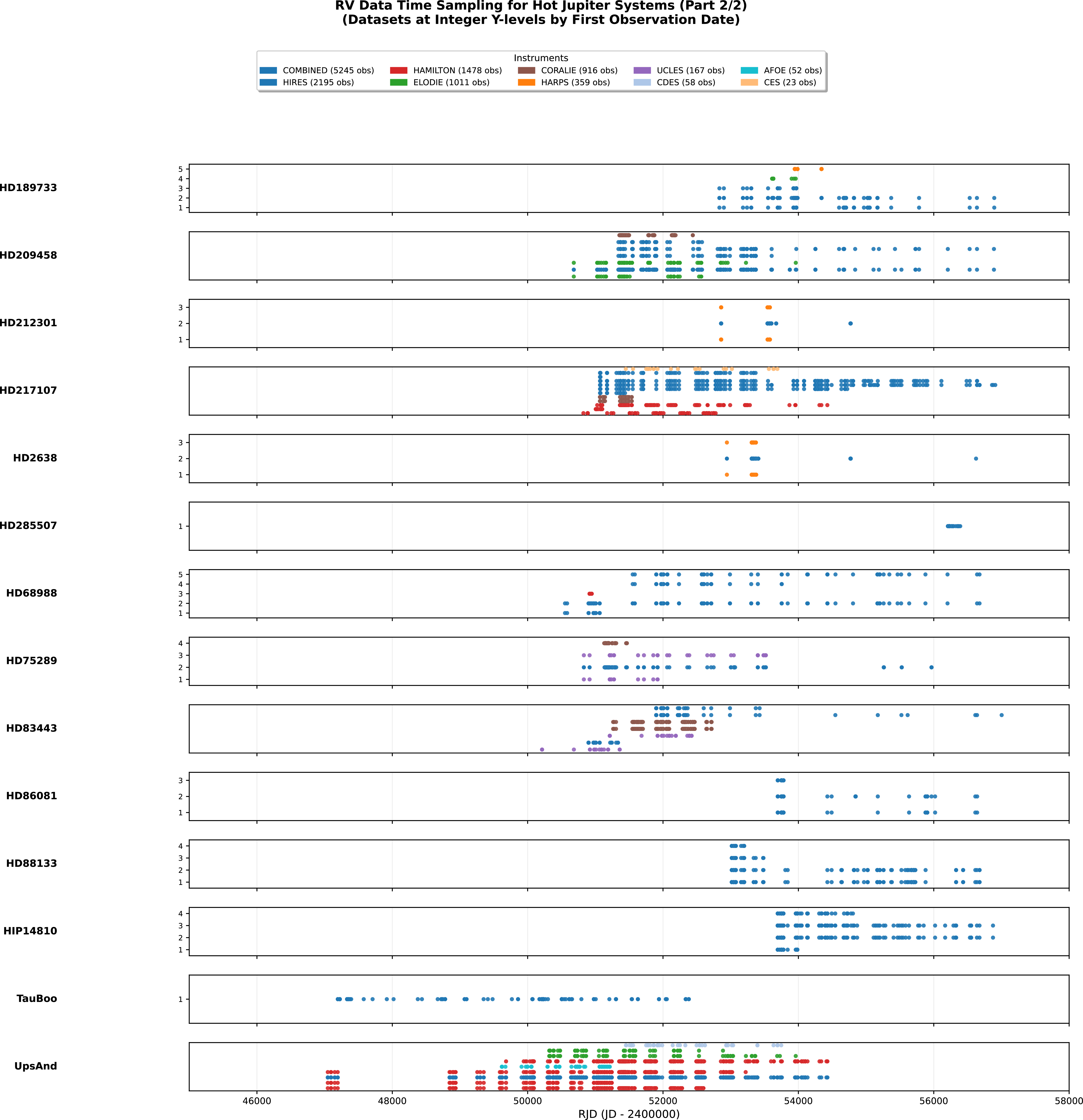
Of the 37 Hot Jupiters discovered using the RV method, just 28 fulfil the criteria of having publicly available data – and thus these 28 planets form the final sample considered in this work. The observational data are summarised in Table 2, and can be graphically visualised in Figures 1 and 2. As expected, the data come from disparate sources and time periods, hence they have offsets and gaps as visualised in Figures 1 and 2. Such features can affect the detectability of further planets; these subtleties have been explored in detail by other work (e.g. Wittenmyer et al. Reference Wittenmyer2013; Lagrange et al. Reference Lagrange2023; Li et al. Reference Li, Kane, Blunt and Harada2025). The main characteristics of the spectrographs selected for this analysis are summarised in Table 3.
The distribution of RV data used in this work over time for the selected targets (part 1). The instrumental precision of this data, along with additional data, are presented in Table 2.

The distribution of RV data used in this work over time for the selected targets (part 2). The instrumental precision of this data, along with additional data, are presented in Table 2.

We note that we have carried out additional observations of HD 83443 using Minerva-Australis (Wittenmyer et al. Reference Wittenmyer2018; Addison et al. Reference Addison2019, Reference Addison2021; Errico et al. Reference Errico2022) in the time since the 18-yr Anglo-Australian Planet Search (Tinney et al. Reference Tinney2001; Butler et al. Reference Butler2001; Wittenmyer et al. Reference Wittenmyer2014) ceased operation. Those data amount to 22 observations between 8 February 2019 to 22 February 2021.
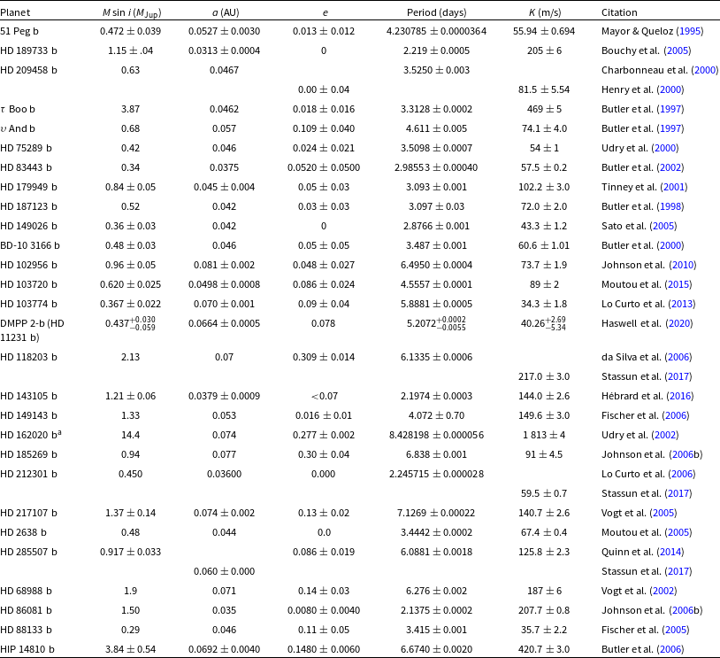
Table 4 summarises the stellar parameters for our 28 target stars. Table 5 shows the planetary parameters of the Hot Jupiter for each of our targets. The host stars considered here are generally mature Solar-type dwarfs, reflecting the selection biases of RV surveys. The specific selection functions of the multifarious RV surveys included herein are beyond the scope of this work – but in general they tend to select solar type, quiet, single stars as represented in Table 4. Such stars are therefore well-represented in the exoplanet demographics literature, with cold giant planets found to orbit $\sim$
10% of them (e.g. Cumming et al. Reference Cumming2008; Wittenmyer et al. Reference Wittenmyer2011a; Zechmeister et al. Reference Zechmeister2013; Bryan et al. Reference Bryan2016; Wittenmyer et al. Reference Wittenmyer2016; Nielsen et al. Reference Nielsen2019; Poleski et al. Reference Poleski2021; Gan et al. Reference Gan2024). The effect of the presence of a Hot Jupiter on the occurrence rate of Cold Jupiters is unexplored and is the main aim of this work.
$\sim$
10% of them (e.g. Cumming et al. Reference Cumming2008; Wittenmyer et al. Reference Wittenmyer2011a; Zechmeister et al. Reference Zechmeister2013; Bryan et al. Reference Bryan2016; Wittenmyer et al. Reference Wittenmyer2016; Nielsen et al. Reference Nielsen2019; Poleski et al. Reference Poleski2021; Gan et al. Reference Gan2024). The effect of the presence of a Hot Jupiter on the occurrence rate of Cold Jupiters is unexplored and is the main aim of this work.
3. Methodology
In this section, we describe the two main analysis procedures employed to assess the current and future detectability of long-period ‘acquaintances’ to the known Hot Jupiters studied in this work. First, we examine the sensitivity afforded by the existing data. Then, we perform a suite of simulations under various scenarios of instrumental precision, observing cadence, and temporal baseline. Taken together, these analyses reveal the extent of our knowledge about such cold giant companions and inform the observational strategies required to probe the outer reaches of these planetary systems.
3.1. Existing data
To assess the sensitivity of the existing data to Cold Jupiters, we conducted injection-recovery tests using RVSearch (Rosenthal et al. Reference Rosenthal2021), a Python package built on top of RadVel (Fulton et al. Reference Fulton, Petigura, Blunt and Sinukoff2018). The algorithm injects synthetic planetary signals, with orbital periods and minimum masses ( $m \sin i$
) drawn from log-uniform distributions, eccentricities that are drawn from a beta distribution (Kipping Reference Kipping2013), and the argument of periapsis drawn from uniform distribution between 0 and 360
$m \sin i$
) drawn from log-uniform distributions, eccentricities that are drawn from a beta distribution (Kipping Reference Kipping2013), and the argument of periapsis drawn from uniform distribution between 0 and 360 $^\circ$
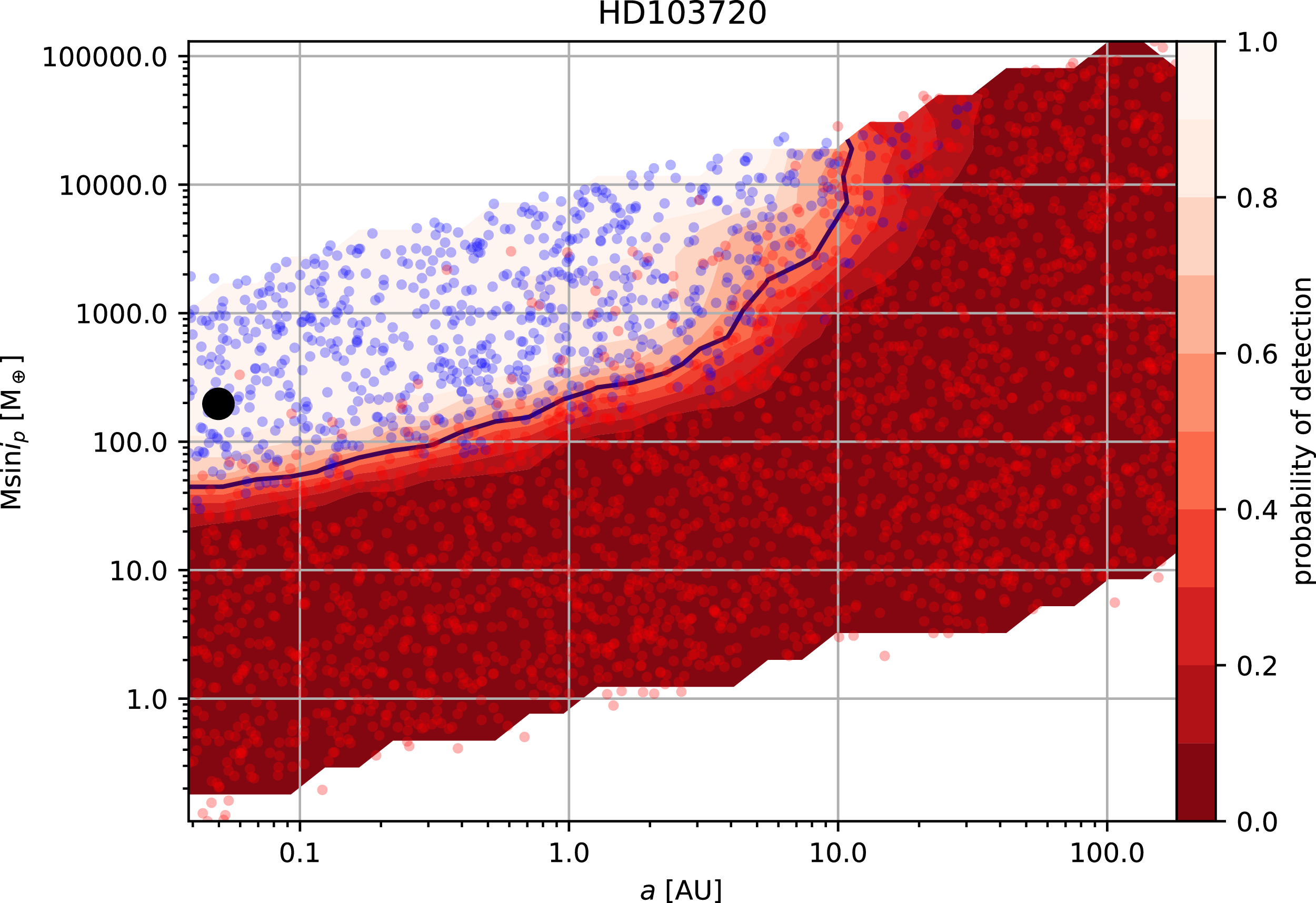
. It is assumed that the orbits of the planets are co-planar in this injection analysis. RVSearch then attempts to recover each injected signal, estimating the detection probability for planets across a range of parameters. As a graphic output, the algorithm produces a completeness contour plot featuring two clearly distinct regions, as illustrated for HD 103720 in Figure 3.
$^\circ$
. It is assumed that the orbits of the planets are co-planar in this injection analysis. RVSearch then attempts to recover each injected signal, estimating the detection probability for planets across a range of parameters. As a graphic output, the algorithm produces a completeness contour plot featuring two clearly distinct regions, as illustrated for HD 103720 in Figure 3.
Instrumental parameters of selected Telescopes.

Stellar parameters of selected host stars. For consistency, all parameters listed here are sourced from Sousa et al. (Reference Sousa2021), though we note that they have been rounded for ease of reading.

RVSearch has become a widely adopted tool in the exoplanet community, particularly for evaluating survey completeness and population-level detection efficiencies (Howard & Fulton Reference Howard and Fulton2016; Fulton et al. Reference Fulton, Petigura, Blunt and Sinukoff2018; Rosenthal et al. Reference Rosenthal2021). Its performance has been validated across diverse RV datasets (e.g. Polanski et al. Reference Polanski2024; Zhang et al. Reference Zhang2025; Van Zandt et al. Reference Van Zandt2025), and it has been instrumental in quantifying detection biases and uncovering the parameter space accessible to current surveys (e.g. Laliotis et al. Reference Laliotis2023; Harada et al. Reference Harada2024b; Wittenmyer et al. Reference Wittenmyer2025). A detailed technical description of the algorithm, including its treatment of multi-instrument datasets and inter-dataset offsets, is provided in Rosenthal et al. (Reference Rosenthal2021), to which we refer the reader for full details. For our analysis, we employed the standard RVSearch configuration, with 3 000 injected trial signals per star to ensure convergence of the completeness estimates. Tests with larger numbers of injections yielded consistent results, supporting the robustness of this choice, but proved to be prohibitively computationally intensive for such injection numbers to be used for our full analysis. Poorly sampled or highly eccentric orbital configurations are naturally incorporated into the injection–recovery framework, and their contribution to the overall completeness is therefore properly accounted for.
3.2. Simulated data
To inform the observational strategy, we tested nine scenarios in a $3\times 3$
grid of (low, medium, high) cadenceFootnote
e
and (low, medium, high) RV measurement precision. We define these categories of measurement precision by representative instruments: ‘low’ – Minerva-Australis (Addison et al. Reference Addison2019), ‘medium’ – Keck/HIRES (Vogt et al. Reference Vogt1994), ‘high’ – VLT/ESPRESSO (Pepe et al. Reference Pepe2014). We wish to test the relative importance of precision and cadence for this science goal, and these values of cadence and precision for the simulated observations are chosen to bracket the range of typical RV survey programmes. Clearly, one would like to observe at the highest cadence and the highest precision, but the realities of telescope time allocation preclude such a scenario. In general, precision and cadence (i.e. the amount of time available) are inversely related. Small telescopes, such as those that make up the Minerva-Australis array (Addison et al. Reference Addison2019), can dedicate a great deal of time to such a project, whereas larger telescopes with more in-demand instruments (e.g. Keck/HIRES, VLT/ESPRESSO) would naturally be under far more competitive pressure, limiting the available time.
$3\times 3$
grid of (low, medium, high) cadenceFootnote
e
and (low, medium, high) RV measurement precision. We define these categories of measurement precision by representative instruments: ‘low’ – Minerva-Australis (Addison et al. Reference Addison2019), ‘medium’ – Keck/HIRES (Vogt et al. Reference Vogt1994), ‘high’ – VLT/ESPRESSO (Pepe et al. Reference Pepe2014). We wish to test the relative importance of precision and cadence for this science goal, and these values of cadence and precision for the simulated observations are chosen to bracket the range of typical RV survey programmes. Clearly, one would like to observe at the highest cadence and the highest precision, but the realities of telescope time allocation preclude such a scenario. In general, precision and cadence (i.e. the amount of time available) are inversely related. Small telescopes, such as those that make up the Minerva-Australis array (Addison et al. Reference Addison2019), can dedicate a great deal of time to such a project, whereas larger telescopes with more in-demand instruments (e.g. Keck/HIRES, VLT/ESPRESSO) would naturally be under far more competitive pressure, limiting the available time.
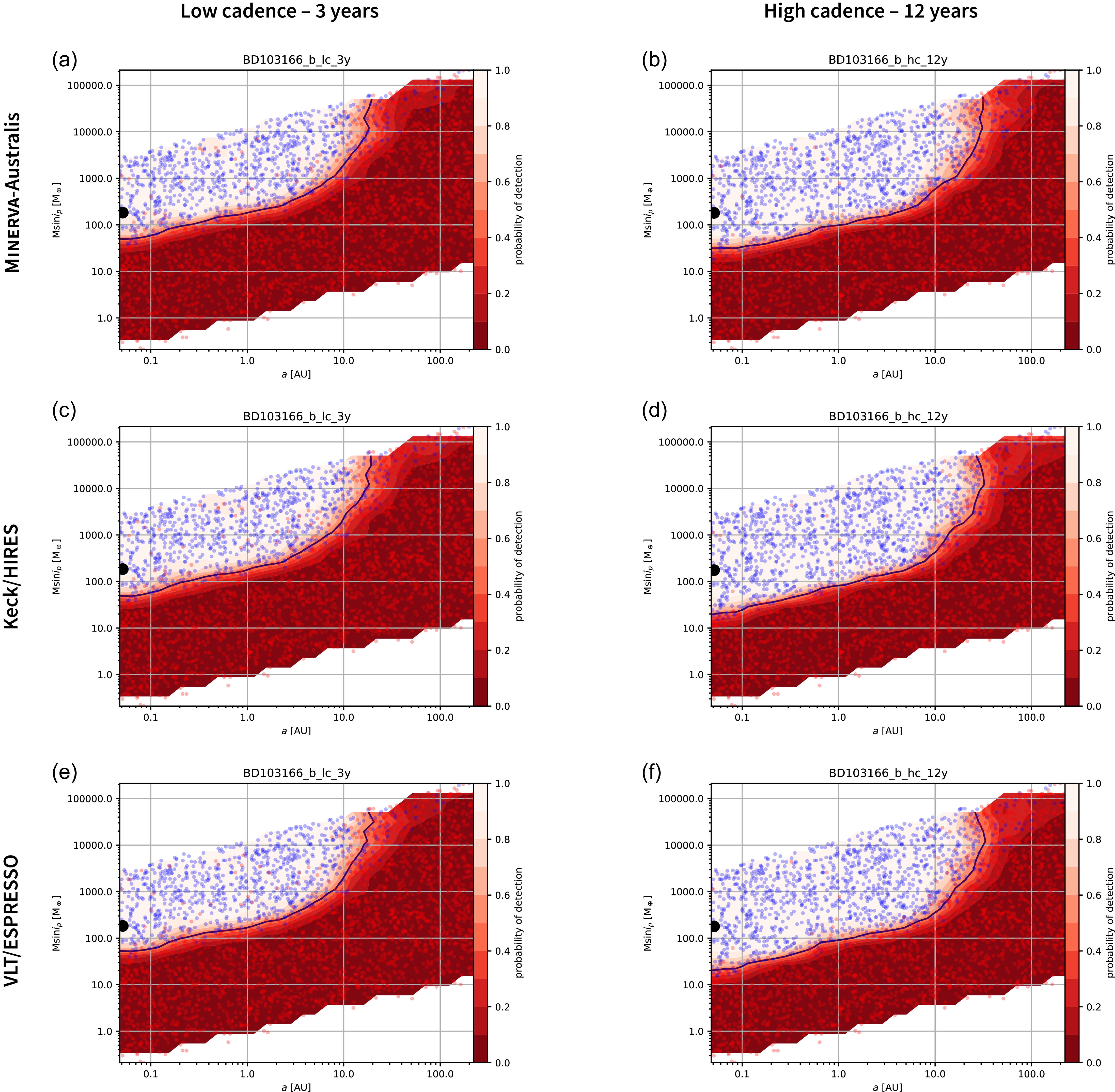
To test the relative importance of these factors, we simulate observing campaigns for the 28 stars examined herein. We also test three different temporal baselines for the new observations: 3, 6, and 12 yr. The purpose is to determine the degree to which the observational baseline can overcome lower cadence and/or instrumental precision. The final result is a set of 27 total observing scenarios for each of our 28 selected systems. Since it is not possible to include such a large number of figures, we include Figure 5 to illustrate the improvement in detection when comparing low- and high-cadence observations for the three selected telescopes. Again, it is obvious that the highest cadence, at the highest precision, for the longest time, will always produce the best results. Our purpose here is to provide a matrix of possibilities to inform and optimise observing strategies to address the science goal of measuring the occurrence rate of Hot Jupiter–Cold Jupiter pairs.
Orbital parameters of Hot Jupiter exoplanets used in this work. For each system, we present the parameters as derived in the discovery work, for consistency. Where the discovery work does not provide a given parameter, we give the value presented by the next available work, for completeness. Where no uncertainties were presented, we give the value as published. We note that these numbers are presented solely for the benefit of the reader, as our analysis fully refit each system rather than assuming a prior published orbit for known planets.

aWe note here that the mass determined for HD 162020 b in the discovery work is greater than 13 M $_{Jup}$
, and, as such, that object might well be considered to be a brown dwarf rather than a giant planet. Regardless of its true nature, we have included the system in this work for completeness. It should also be noted that more recent work (Stassun et al. Reference Stassun, Collins and Gaudi2017) obtains a planetary mass for this object, at M sin i of 9.840
$_{Jup}$
, and, as such, that object might well be considered to be a brown dwarf rather than a giant planet. Regardless of its true nature, we have included the system in this work for completeness. It should also be noted that more recent work (Stassun et al. Reference Stassun, Collins and Gaudi2017) obtains a planetary mass for this object, at M sin i of 9.840 $\pm$
2.750 M
$\pm$
2.750 M $_\mathrm{Jup}$
.
$_\mathrm{Jup}$
.
RVSearch completeness contour plot for HD 103720. The large black dot represents the periodic signal identified by RVSearch (i.e. the known planet). The small points denote injected synthetic planets. Blue points correspond to recovered signals, while red points were not recovered. Red contours show the detection probability, averaged over small bins in semi-major axis and $m \sin i$
space. The black line marks the 50% detection probability contour.
$m \sin i$
space. The black line marks the 50% detection probability contour.

We generated simulated RVs using the fitted parameters of the known planet(s) to produce Keplerian orbits, to which noise was added. The value of the noise was drawn with replacement from the residuals of a fit to the known planet(s) performed with the DACE tool (Fulton et al. Reference Fulton, Petigura, Blunt and Sinukoff2018). We draw the uncertainty of each simulated measurement from a Gaussian distribution with means and standard deviation as follows in units of ${\mathrm{m\,s^{-1}}}$
: ‘low precision’:
${\mathrm{m\,s^{-1}}}$
: ‘low precision’: $\mu$
= 10 and
$\mu$
= 10 and $\sigma$
= 2; ‘medium precision’:
$\sigma$
= 2; ‘medium precision’: $\mu$
= 3 and
$\mu$
= 3 and $\sigma$
= 0.6; ‘high precision’:
$\sigma$
= 0.6; ‘high precision’: $\mu$
= 0.5 and
$\mu$
= 0.5 and $\sigma$
= 0.1. These were chosen to approximate, respectively, instruments akin to MINERVA and Minerva-Australis (Swift et al. Reference Swift2015; Wilson et al. Reference Wilson2019; Addison et al. Reference Addison2019), Keck/HIRES (Vogt et al. Reference Vogt1994), and VLT/ESPRESSO (Pepe et al. Reference Pepe2014). Hereafter we refer to these instruments by name as exemplars of the three levels of measurement precision tested.
$\sigma$
= 0.1. These were chosen to approximate, respectively, instruments akin to MINERVA and Minerva-Australis (Swift et al. Reference Swift2015; Wilson et al. Reference Wilson2019; Addison et al. Reference Addison2019), Keck/HIRES (Vogt et al. Reference Vogt1994), and VLT/ESPRESSO (Pepe et al. Reference Pepe2014). Hereafter we refer to these instruments by name as exemplars of the three levels of measurement precision tested.
4. Results
In this section, we present the results of our detection sensitivity analysis for the currently available data, then show the results of the simulated scenarios to illustrate the effectiveness of various instruments and observing strategies.
4.1. Sensitivity of existing data to cold giant companions
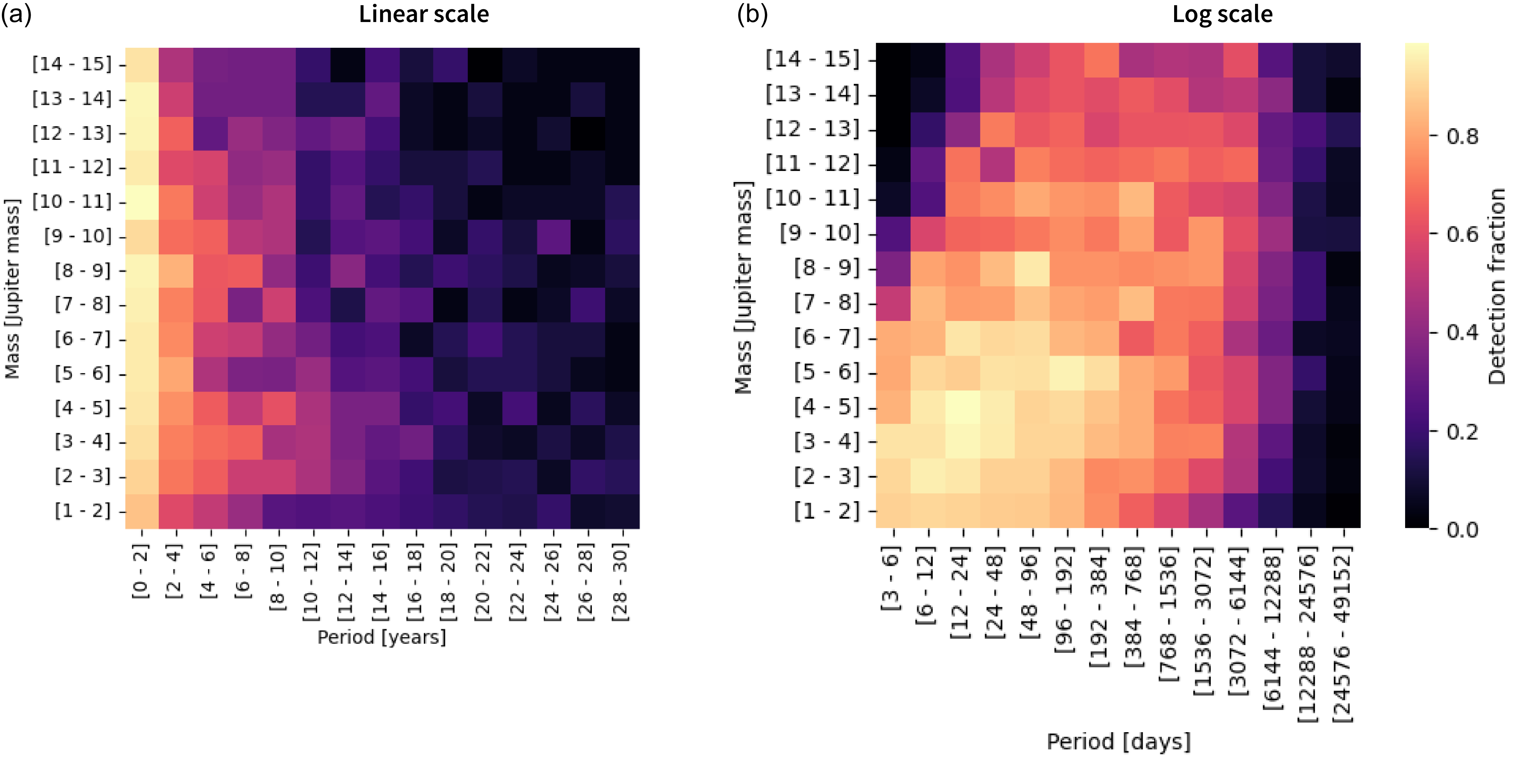
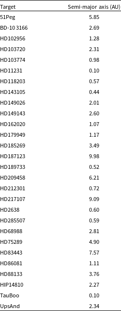
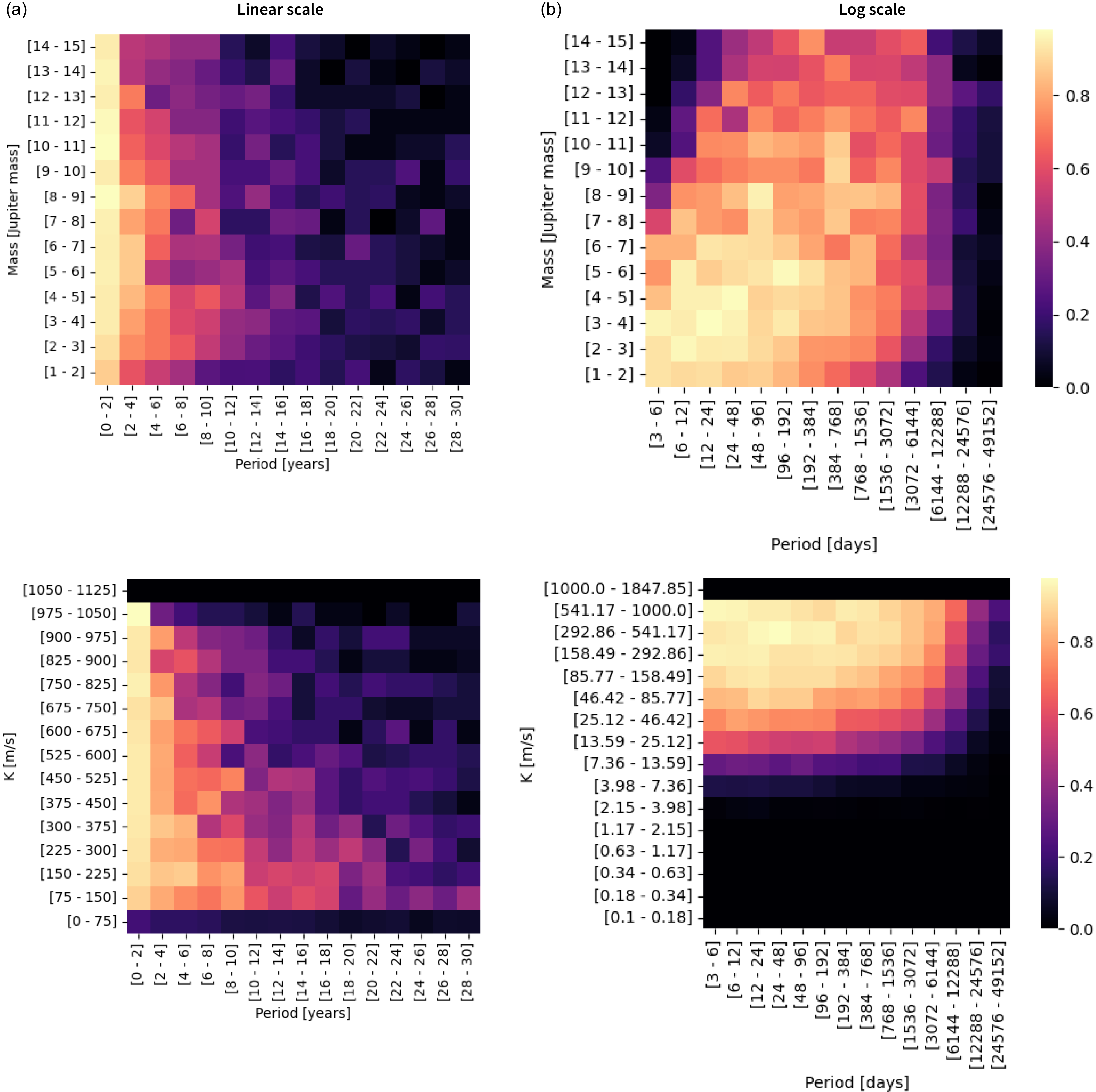
Despite these being well-studied and bright Hot Jupiter hosts, the existing data are remarkably ineffective at detecting Cold Jupiters (Table 6). Figure 4 shows the detection sensitivity for Cold Jupiters averaged over our 28 Hot Jupiter systems. From these results, we see that in general, 49.91% of Cold Jupiters beyond 3 au ( $P\sim$
5 yr) could be detected with the currently available data. To aid in interpreting the heat maps in this Section, we note that the typical uncertainty of the location of the RVSearch 50% recovery boundary (as denoted by the thick black line in Figure 3) is about 10% in semimajor axis space. Furthermore, it is worth noting that RVSearch correctly identified the known Hot Jupiter in 98.8% of trials.
$P\sim$
5 yr) could be detected with the currently available data. To aid in interpreting the heat maps in this Section, we note that the typical uncertainty of the location of the RVSearch 50% recovery boundary (as denoted by the thick black line in Figure 3) is about 10% in semimajor axis space. Furthermore, it is worth noting that RVSearch correctly identified the known Hot Jupiter in 98.8% of trials.
Zink & Howard (Reference Zink and Howard2023) presented a completeness-corrected occurrence rate for Hot Jupiter–Cold Jupiter pairs of nearly 100%, with a steeply rising power-law towards longer periods. The extremely low completeness shown in our sample is consistent with this interpretation: that such ‘acquaintances of Hot Jupiters’ should be common (approaching 100%) but a great many have so far been missed. To better understand these systems and their architectures, it is therefore profitable to continue to observe these systems. In the next subsection, we show the results of our simulated observing strategies designed to identify the most efficient route to reveal the population of these cold companions lurking in the outer darkness.
4.2. Nine future observation scenarios for three different exoplanet observation facilities
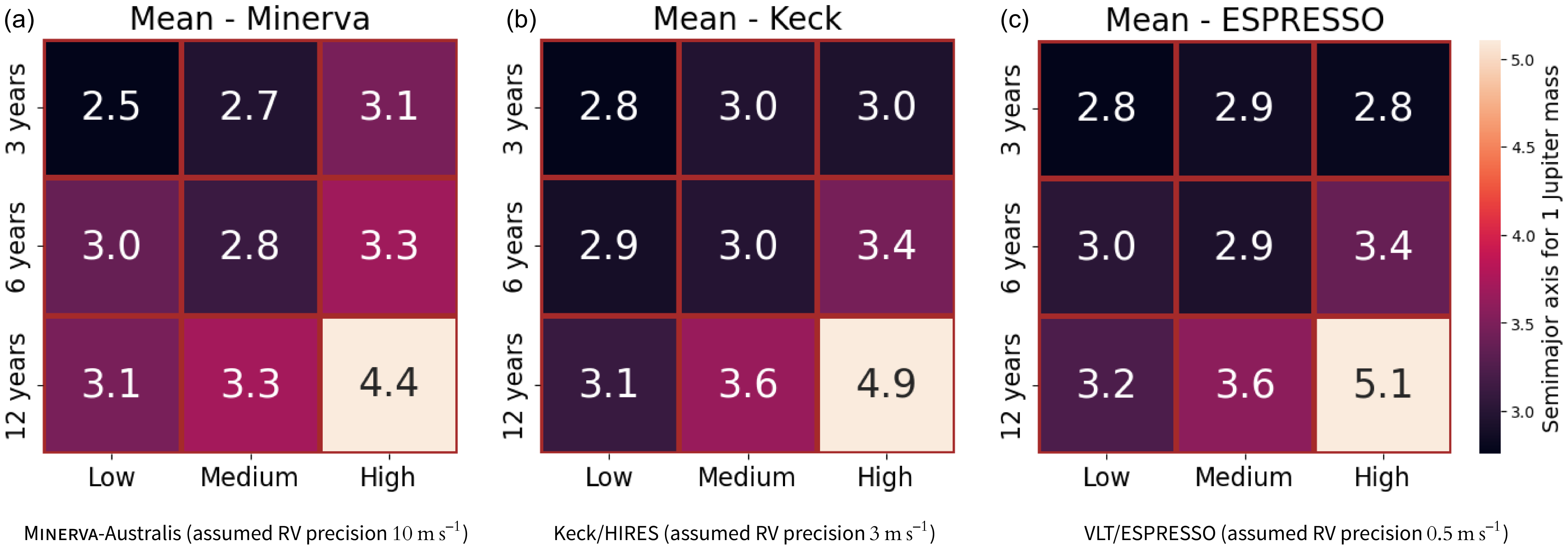
In Figure 6, we summarise the results of our simulated scenarios for each of the three observatories considered in this work (MINERVA/Minerva-Australis, Keck/HIRES, and VLT/ESPRESSO). In each panel, we present a three-by-three grid showing the semi-major axis at which the facility has a 50% chance of recovering a 1 $M_\mathrm{Jup}$
planet for each combination of observing cadence (low, medium, high) and baseline of additional observations (3, 6, or 12 yr).Footnote
f
Each box represents the mean semi-major axis across the 28 stars in our sample. The three facilities in the figure are characterised by assumed instrumental RV precisions of
$M_\mathrm{Jup}$
planet for each combination of observing cadence (low, medium, high) and baseline of additional observations (3, 6, or 12 yr).Footnote
f
Each box represents the mean semi-major axis across the 28 stars in our sample. The three facilities in the figure are characterised by assumed instrumental RV precisions of $10\,{\mathrm{m\,s^{-1}}}$
for Minerva-Australis – Figure 6(a);
$10\,{\mathrm{m\,s^{-1}}}$
for Minerva-Australis – Figure 6(a); $3\,{\mathrm{m\,s^{-1}}}$
for Keck/HIRES – Figure 6(b); and
$3\,{\mathrm{m\,s^{-1}}}$
for Keck/HIRES – Figure 6(b); and $0.5\,{\mathrm{m\,s^{-1}}}$
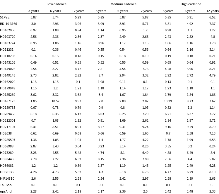
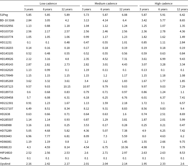
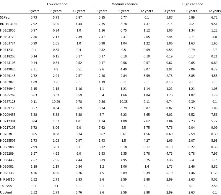
for VLT/ESPRESSO – Figure 6(c). /hlFor reference, the complete data for each telescope, for each combination of cadence and duration are given in Tables 7–9.
$0.5\,{\mathrm{m\,s^{-1}}}$
for VLT/ESPRESSO – Figure 6(c). /hlFor reference, the complete data for each telescope, for each combination of cadence and duration are given in Tables 7–9.
Heat maps showing the detection efficiency for exoplanet candidates injected to the existing observational radial velocity data for 28 known Hot Jupiter host stars. A total of 3 000 unique potential candidate companions were injected, one at a time, for each star considered, with masses and orbital periods each drawn from a log-normal distribution. In both panels, the colour of a square denotes the detection efficiency for a planet in that square – the mean of the detection efficiencies (number of detections divided by the number of injected planets) across the sample of 28 stars. The left panel shows the data as a function of orbital period, whilst the right shows the same data as a function of log(period). It is clear that planets are most easily detected at short orbital periods, with true Jupiter and Saturn analogues ( $P\sim$
12 and 29 yr, respectively) challenging to detect based on current data. The ‘void’ at the top left of the right-hand panel is an artefact of the injection-recovery process; the signals injected by RVSearch all had radial velocities of less than 1 000 ms
$P\sim$
12 and 29 yr, respectively) challenging to detect based on current data. The ‘void’ at the top left of the right-hand panel is an artefact of the injection-recovery process; the signals injected by RVSearch all had radial velocities of less than 1 000 ms $^{-1}$
. As a result, no planets were generated in the region of the ‘void’, and so recovery of planets in that region was impossible as there were none to recover.
$^{-1}$
. As a result, no planets were generated in the region of the ‘void’, and so recovery of planets in that region was impossible as there were none to recover.

Comparison of different instruments and observing strategies. It can be noted that the line corresponding to 50% detection shifts downward and to the right as both the cadence and duration increase. Although subtle, differences are also seen between telescopes due to varying measurement precision.

The first detail to notice is that for lower cadence and shorter duration, the semi-major axis at which a 1 $M_\mathrm{Jup}$
planet is detectable is smaller than for scenarios with higher cadence and longer duration, as one would intuitively expect. The second detail regarding the comparison of telescopes is that the highest-precision instrument detects a 1
$M_\mathrm{Jup}$
planet is detectable is smaller than for scenarios with higher cadence and longer duration, as one would intuitively expect. The second detail regarding the comparison of telescopes is that the highest-precision instrument detects a 1 $M_\mathrm{Jup}$
planet at a larger semi-major axis than lower-precision instruments for a given combination of cadence and duration; this is again consistent with expectations. However, it is perhaps surprising to note that the gains made from greatly improved RV precision are only small, compared to those accrued as a result of longer baselines or higher observation cadence.
$M_\mathrm{Jup}$
planet at a larger semi-major axis than lower-precision instruments for a given combination of cadence and duration; this is again consistent with expectations. However, it is perhaps surprising to note that the gains made from greatly improved RV precision are only small, compared to those accrued as a result of longer baselines or higher observation cadence.
Indeed, it is particularly interesting that the detection semi-major axis achieved by the facility with the lowest RV precision (Minerva-Australis) for combinations of higher cadence and longer durations equals or exceeds the performance of more precise instruments at lower cadence and/or shorter durations. These results show that the disadvantage of lower measurement precision can be compensated for by higher cadence – demonstrating the ongoing value of ‘regular’ RV observations in an extreme-precision (EPRV) world. In other words, an VLT/ESPRESSO-like EPRV instrument may deliver measurement precision 10–20 times better than a Minerva-Australis-like facility, but, when those facilities are used to search for Cold Jupiters, the ‘lesser’ (and more accessible) facility achieves the desired outcome.
Semi-major axes (in AU) at which 50% of 1 $M_\mathrm{J}$
planets would be detected, should they be present in the system in question, based upon an injection-recovery analysis of the currently available radial velocity data. The data reveals significant differences in our ability to detect Cold Jupiters across this population of 28 stars for which long-period radial velocity data are available.
$M_\mathrm{J}$
planets would be detected, should they be present in the system in question, based upon an injection-recovery analysis of the currently available radial velocity data. The data reveals significant differences in our ability to detect Cold Jupiters across this population of 28 stars for which long-period radial velocity data are available.

For each star (and each scenario), RVSearch produces a table containing the orbital parameters of the injected signals (planets) and whether they were recovered. We considered the space defined by planet mass and period and divided it into ‘boxes’ (for example, intervals of one Jupiter mass and two years). As an illustration, the first box (located at the bottom left of the heat map in Figure 4) spans from 1 to 2 Jupiter masses and from 0 to 2 yr. The right panel (Figure 4) shows the same result on a log scale.
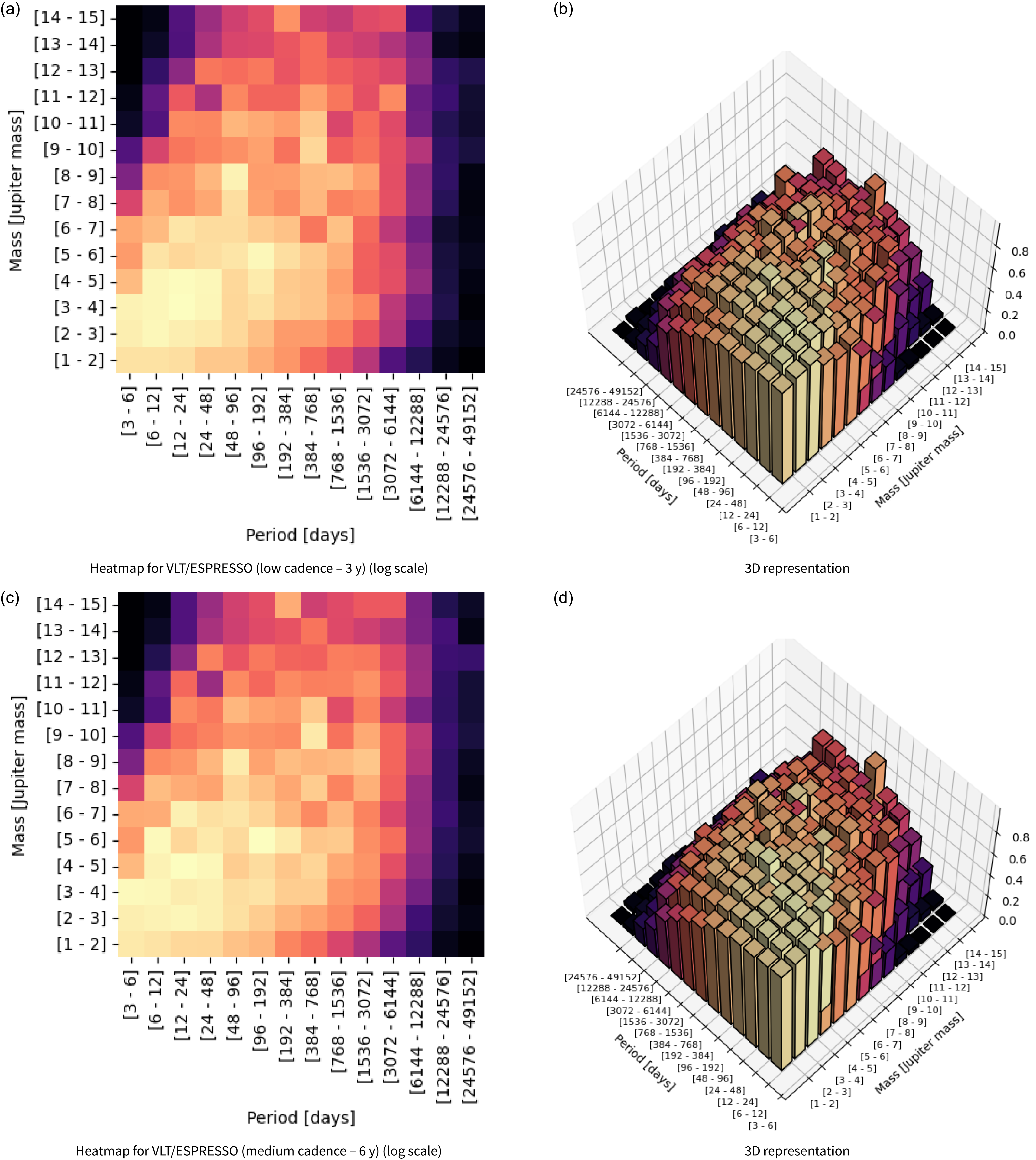
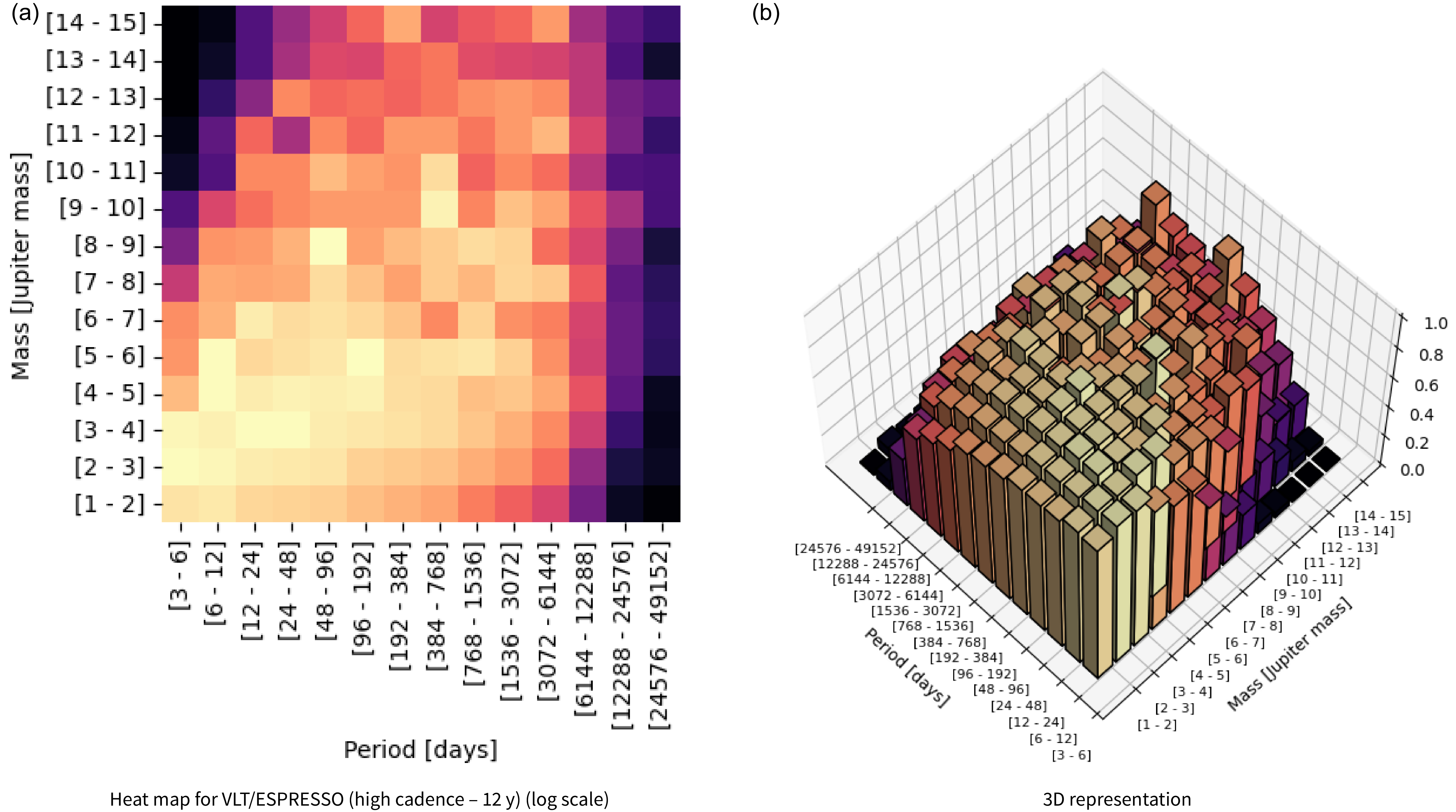
It is interesting to directly compare the characteristics of the real observational data (presented in Figure 4) and the simulated data (Figure 7). The high degree of similarity between the two figures is encouraging – revealing that the simulated data has very similar characteristics to the real data. In other words, this suggests that the methodology behind the creation of the simulated data is robust and accurately reflects the reality of the observations made.
For each mass–period box, we computed the ratio of detected to injected signals (this ratio is always less than or equal to 1) and visualised the results as a heat map. This process yielded 756 heat maps, which we then averaged box-by-box across all stars, resulting in 9 heat maps that represent the average detection rates over the 28 stars.
4.3. VLT/ESPRESSO/Minerva performance comparison
In the previous sections, we have considered the benefits of a variety of observational strategies in the search for Cold Jupiters for three different types of exoplanet search facilities – those with low RV precision (analogues to the Minerva-Australis array), with medium precision (like data obtained using Keck), and those with high precision (‘extreme precision radial velocity’ or ‘EPRV’) such as VLT/ESPRESSO). We have clearly shown that longer observational baselines are the key to detecting distant massive planets using RV observations, regardless of the facility involved. Our results also reveal that increasing the observational cadence leads to the more efficient detection of Cold Jupiters in the vast majority of cases. In general, we also find that the use of high-precision facilities yields only marginal gains over the results obtained by smaller, more accessible telescopes (see e.g. Figure 6). In this section, we therefore address the question: can the long-term performance of large, highly accurate telescopes in the search for Jupiter-like planets be matched by smaller, more accessible, and more affordable facilities?
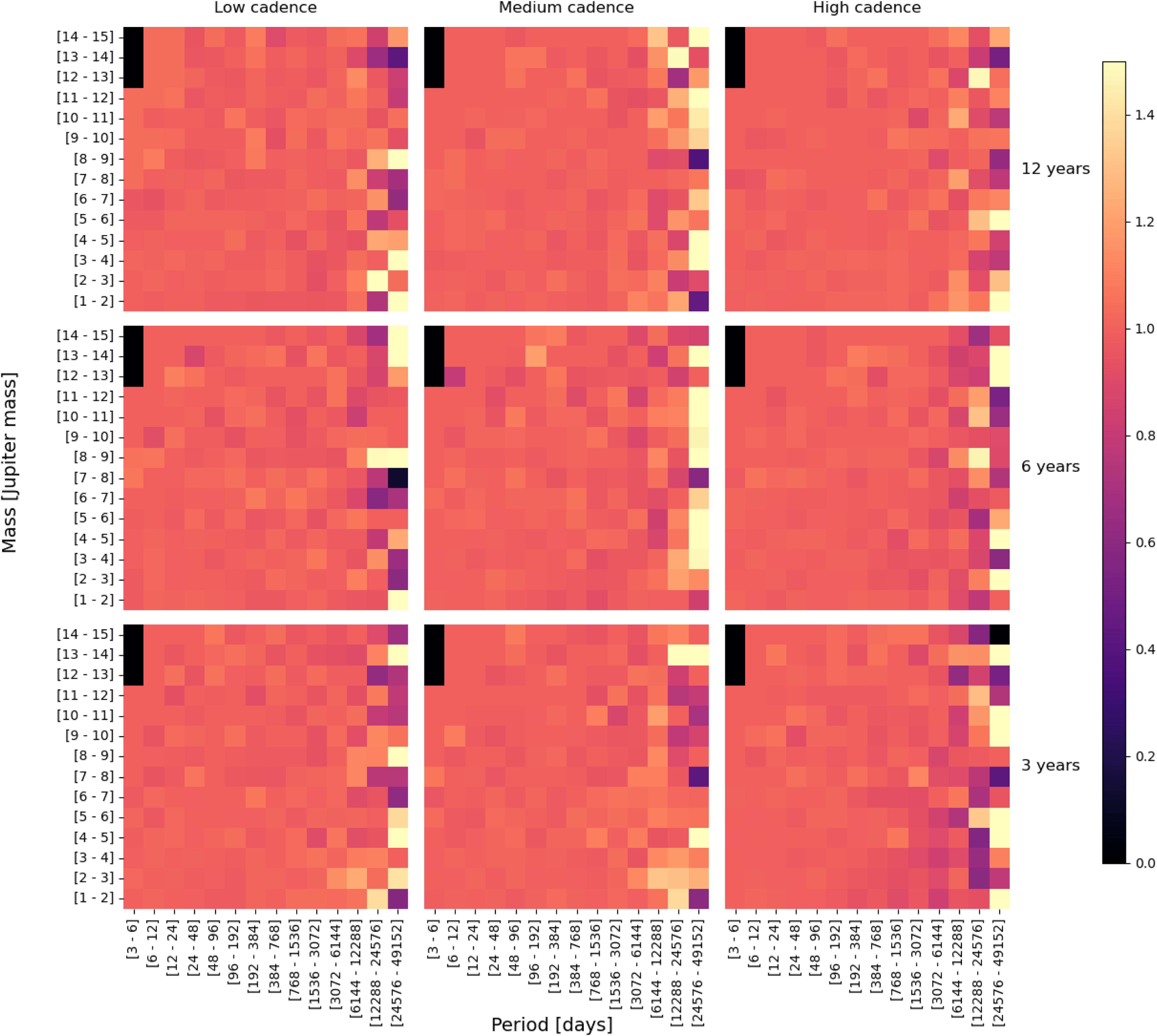
To address this, we consider our two extreme cases – VLT/ESPRESSO (high precision) and Minerva-Australis (low precision). Rather than simply considering the detection efficiencies of the two facilities on their own, we look to make two direct comparisons. In the first, we calculate the ratio of successful detections made by VLT/ESPRESSO to those made using Minerva-Australis – in other words, we divide the detection efficiency of one facility by the other. The results of this comparison are shown in Figure 10. In that Figure, a value of 1.0 denotes that the two facilities perform equally well. If the value is less than 1.0 (represented by reddish to black shades in the colour scale of Figure 10), then Minerva-Australis outperforms VLT/ESPRESSO, whilst values greater than 1.0 (the lighter shades in Figure 10) denote VLT/ESPRESSO outperforming Minerva-Australis. Looking at Figure 10, it is evident that both telescopes perform equally well across the majority of the phase-space considered. The right side of each plot initially appears to highlight areas where performance differences become significant, with numerous dark-shaded regions – particularly in the last column, which corresponds to high-cadence observations. The results in this region should, however, be treated with some caution. This is the region where the detection efficiencies for all three facilities are very low (as can be seen in Figures 7 and 8), and so the variation seen here is most likely simply noise.
The second comparison we make is to take the results calculated above (the ratio of the detection efficiencies of the two facilities) and scale the result by the ratio of the cost of the two facilities, as detailed in Equation 1. VLT/ESPRESSOFootnote g is a high-performance but very expensive facility compared to Minerva-AustralisFootnote h (European Southern Observatory n.d.), and so it is interesting to consider the cost-effectiveness of the two types of facility as tools to search for Cold Jupiters.
 \begin{align} \left(\frac{\text{\$VLT/ESPRESSO}}{\text{\$Minerva}}\right) \times \left(\frac{\# \text{Minerva}}{\# \text{VLT/ESPRESSO}}\right)\end{align}
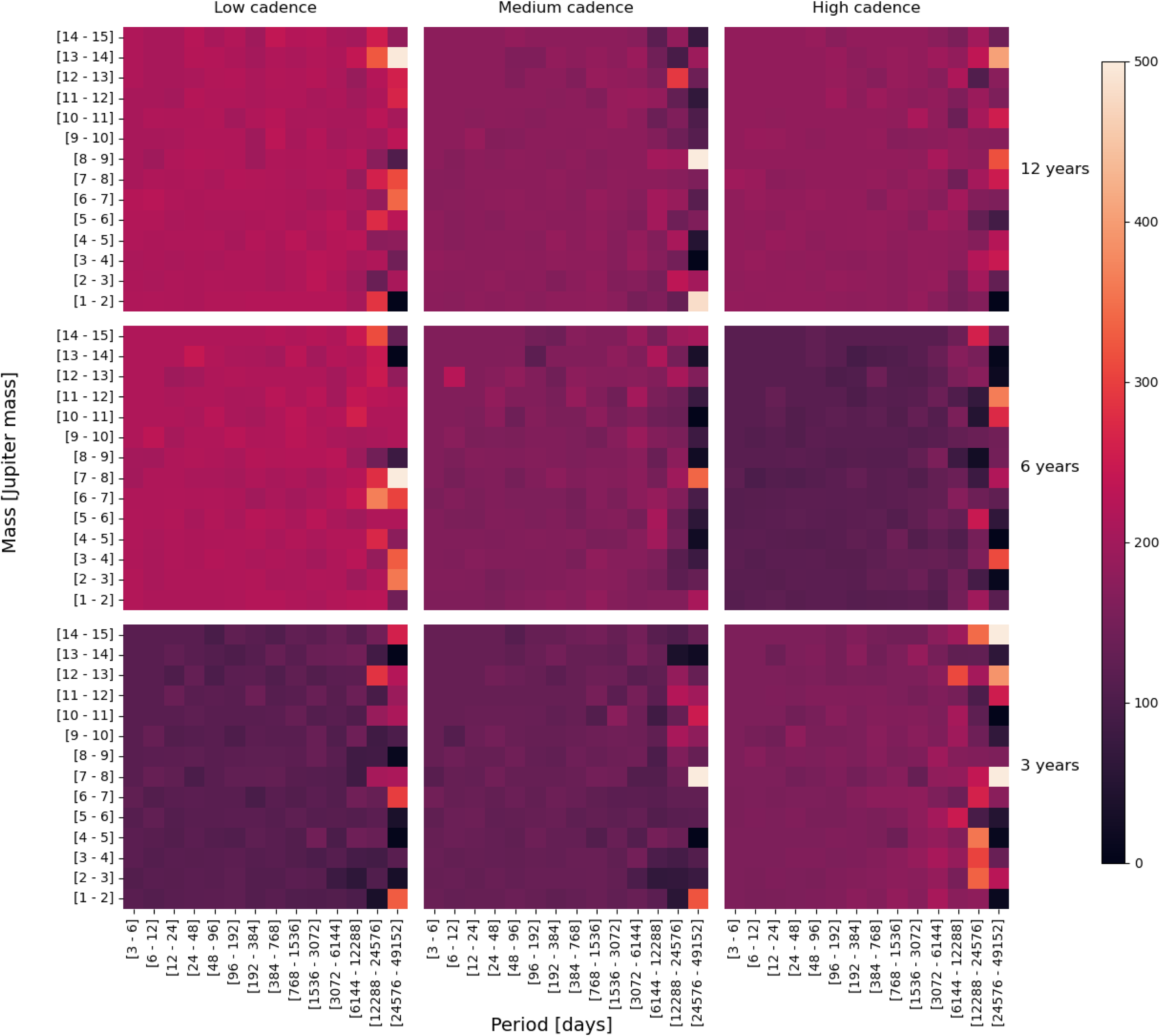
This equation equals 1 when Minerva-Australis is as cost-effective as VLT/ESPRESSO, whilst values greater than 1 indicate that Minerva-Australis provides better value for money (not in absolute performance, but in cost per detection). We present the results of this analysis in Figure 11, where it can be clearly seen that Minerva-Australis represents a far more cost-effective tool for searching for Cold Jupiters than the more expensive facility. This is not a surprise – both facilities are broad equally efficient as tools for the detection of Cold Jupiters, and so it makes sense that the cheaper facility would be more cost-effective. Once again, the noisy results in the right-hand columns in Figure 11 are purely the result of the low detection efficiencies for the two facilities at such long orbital periods.
Finally, we note some limitations to the simple comparison of cost-effectiveness we have described here. For example, this approach clearly breaks down for very faint targets where smaller telescopes are unable to obtain useful RV data at all. Another subtlety we have not considered is a ‘hybrid’ observing strategy whereby certain orbital phases disproportionately benefit from higher precision measurements. Such intricacies are beyond the scope of this work; it is clear that in practice, small and large telescopes serve complementary roles for this and other science goals.
5. Conclusions
In this work, we have defined Hot Jupiter–Cold Jupiter ‘siblings’ as planetary systems containing both a Hot Jupiter and a distant outer giant. Motivated by the discovery of the Hot Jupiter–Cold Jupiter ‘siblings’ in the HD 83443 system (Errico et al. Reference Errico2022); we wished to estimate how common such architectures are, given the severe observational biases against detecting these sorts of systems. From a sample of 28 Hot Jupiter systems that had enough RV data to meaningfully contribute to this investigation, we indeed found the detection sensitivity woefully lacking, even for planets of many Jupiter masses. We then performed an extensive suite of simulated observational strategies to determine the way forward in addressing this problem.
Our analysis across nine scenarios and three telescopes reveals several key findings. First, the existing data, despite being gathered from well-studied and bright Hot Jupiter hosts, are generally ineffective at detecting Cold Jupiters, highlighting the challenge of probing these longer-period companions. We suspect that this arises from a human bias: for Hot Jupiter systems, once the short-period planet is well-characterised, the target’s observing priority is reduced or eliminated in favour of other, ‘more interesting’ targets. The result is that Hot Jupiter systems tend to have short baselines of RV data, hindering our quest to understand the occurrence of any planetary siblings.
We also find that, although higher instrumental precision extends sensitivity to larger semi-major axes for a given observing strategy, the total baseline over which an observation campaign is carried out is the dominant factor in our ability to detect Cold Jupiters. We find that the results are relatively insensitive to the RV measurement precision of the facility being used; the performance of a high-cadence, decade-long programme using a low-cost dedicated facility such as Minerva-Australis matches, or even exceeds, that of shorter, lower-cadence observations by a higher cost extreme-precision RV (EPRV) facility such as VLT/ESPRESSO. Indeed, our results show that low-cost dedicated facilities such as Minerva-Australis will prove to be far more cost-effective in delivering discoveries of Cold Jupiters than facilities such as Keck and VLT/ESPRESSO.
Notably, a high-cadence, decade-long Minerva programme can match or exceed the performance of shorter, lower-cadence VLT/ESPRESSO observations, illustrating that modest measurement precision can be compensated for by strategic scheduling. A cost-normalised comparison further demonstrates that smaller, more accessible facilities can deliver superior return per dollar than flagship instruments when optimised for long-term monitoring. Our results emphasise the value of extended, regular RV campaigns for uncovering long-period exoplanets and inform the design of future surveys. This finding underscores the continuing relevance of traditional RV facilities in an era dominated by EPRV instruments.
Cadence vs duration matrices showing the mean semi-major axis at which a 1 $M_\mathrm{Jup}$
planet was detectable 50% of the time for our simulated scenarios, based on the 28 stars in our sample. The three sub-figures (a, b, and c) present results for three exoplanet facilities - Minerva-Australis, Keck/HIRES, and VLT/ESPRESSO, assuming mean RV precisions for those facilities of 10, 3, and 0.5
$M_\mathrm{Jup}$
planet was detectable 50% of the time for our simulated scenarios, based on the 28 stars in our sample. The three sub-figures (a, b, and c) present results for three exoplanet facilities - Minerva-Australis, Keck/HIRES, and VLT/ESPRESSO, assuming mean RV precisions for those facilities of 10, 3, and 0.5 ${\mathrm{m\,s^{-1}}}$
, respectively. In a given sub-figure, we show how the ability of each facility to detect Cold Jupiters is affected by different observation scenarios – temporal baselines for new observations of 3, 6, and 12 yr (y-axis), and various observation cadences through that period (low, medium, and high cadence; x-axis). The colour and value of each tile gives the distance (in AU) at which the facility have a 50% chance of being able to detect a 1
${\mathrm{m\,s^{-1}}}$
, respectively. In a given sub-figure, we show how the ability of each facility to detect Cold Jupiters is affected by different observation scenarios – temporal baselines for new observations of 3, 6, and 12 yr (y-axis), and various observation cadences through that period (low, medium, and high cadence; x-axis). The colour and value of each tile gives the distance (in AU) at which the facility have a 50% chance of being able to detect a 1 $M_\mathrm{Jup}$
planet, averaged across our sample of 28 target stars. It is clear that the ability of each facility to detect such planets improves with higher observation cadence and longer baselines, as expected. Whilst increased RV precision yields some improvements in the detection distance, these improvements are somewhat less pronounced than might be expected.
$M_\mathrm{Jup}$
planet, averaged across our sample of 28 target stars. It is clear that the ability of each facility to detect such planets improves with higher observation cadence and longer baselines, as expected. Whilst increased RV precision yields some improvements in the detection distance, these improvements are somewhat less pronounced than might be expected.

Table showing the semi-major axis (in AU) at which a detection efficiency of 50% is achieved for 1 M $_J$
planets orbiting the 28 targets stars of this study, for a low-precision, Minerva-Australis analogue facility, as a function of the observational baseline and observational cadence used. In general, the longer the observation baseline, the more distant the Jupiter analogues that could be detected, regardless of the observation cadence chosen. However, it is clear that, for most targets, applying a higher cadence yields markedly better results than simply observing with low cadence.
$_J$
planets orbiting the 28 targets stars of this study, for a low-precision, Minerva-Australis analogue facility, as a function of the observational baseline and observational cadence used. In general, the longer the observation baseline, the more distant the Jupiter analogues that could be detected, regardless of the observation cadence chosen. However, it is clear that, for most targets, applying a higher cadence yields markedly better results than simply observing with low cadence.

Table showing the semi-major axis at which a 1 M $_J$
planet would have a 50% probability of detection around our 28 target stars, for observations carried out with a medium-precision exoplanet survey facility, such as Keck/HIRES, as a function of observational cadence and the baseline over which additional observations are carried out. As was the case for a low-precision facility (e.g. Table 7), a longer baseline of observations typically leads to Jupiter analogues being detectable on longer period orbits, with higher cadence observations typically resulting in an improvement in that detection distance over lower cadence observations.
$_J$
planet would have a 50% probability of detection around our 28 target stars, for observations carried out with a medium-precision exoplanet survey facility, such as Keck/HIRES, as a function of observational cadence and the baseline over which additional observations are carried out. As was the case for a low-precision facility (e.g. Table 7), a longer baseline of observations typically leads to Jupiter analogues being detectable on longer period orbits, with higher cadence observations typically resulting in an improvement in that detection distance over lower cadence observations.

The semi-major axes at which a planet of mass 1 M $_J$
would be detected with 50% probability orbiting our 28 target stars, for observations using a high-precision survey facility, such as VLT/ESPRESSO, as a function of observational cadence and the baseline over which observations are performed. As was the case for low- and medium-precision facilities, a longer baseline of observations again leads to Jupiter mass planets being detectable on longer period orbits, with higher cadence observations typically resulting in an improvement in that detection distance over lower cadence observations.
$_J$
would be detected with 50% probability orbiting our 28 target stars, for observations using a high-precision survey facility, such as VLT/ESPRESSO, as a function of observational cadence and the baseline over which observations are performed. As was the case for low- and medium-precision facilities, a longer baseline of observations again leads to Jupiter mass planets being detectable on longer period orbits, with higher cadence observations typically resulting in an improvement in that detection distance over lower cadence observations.

Heat maps showing the detection efficiency of a Minerva-Australis class facility (RV precision $10\,{\mathrm{m\,s^{-1}}}$
) for low cadence observations carried out over a period of three years (i.e. a short temporal baseline). The colour of each square reveals the mean detection probability for a planet in that particular mass and orbital period range, averaged over the 28 star systems studied in this work, based on simulated injection-recovery tests using 3 000 injected planets. The lighter the colour, the greater the mean recovery rate. It is clear that the addition of just three years of low cadence data does not hugely improve our ability to detect Cold Jupiters over the current state of the data (presented in Figure 4), though some small gains are made. The upper panels show the data in planet mass vs orbital period space, whilst the lower ones show the same information plotted in terms of the observed radial velocity, K, and the orbital period of the planet in question. In the upper right panel, it appears that no planets are detected at very high mass for very short periods. This is an artefact of the injection-recovery process used, where RVSearch only injects signals up to a radial velocity of
$10\,{\mathrm{m\,s^{-1}}}$
) for low cadence observations carried out over a period of three years (i.e. a short temporal baseline). The colour of each square reveals the mean detection probability for a planet in that particular mass and orbital period range, averaged over the 28 star systems studied in this work, based on simulated injection-recovery tests using 3 000 injected planets. The lighter the colour, the greater the mean recovery rate. It is clear that the addition of just three years of low cadence data does not hugely improve our ability to detect Cold Jupiters over the current state of the data (presented in Figure 4), though some small gains are made. The upper panels show the data in planet mass vs orbital period space, whilst the lower ones show the same information plotted in terms of the observed radial velocity, K, and the orbital period of the planet in question. In the upper right panel, it appears that no planets are detected at very high mass for very short periods. This is an artefact of the injection-recovery process used, where RVSearch only injects signals up to a radial velocity of $1\,000\,{\mathrm{m\,s^{-1}}}$
. At the shortest orbital periods injected, this ceiling results in a maximum possible planet mass of
$1\,000\,{\mathrm{m\,s^{-1}}}$
. At the shortest orbital periods injected, this ceiling results in a maximum possible planet mass of $\lt 10\textit{M}_J$
– and so that apparent void in detections is simply a location where no planets are injected. This ceiling is clearly seen in the lower right-hand panel, showing that the highest velocity planets are very efficiently detected at short orbital periods, just as one would expect.
$\lt 10\textit{M}_J$
– and so that apparent void in detections is simply a location where no planets are injected. This ceiling is clearly seen in the lower right-hand panel, showing that the highest velocity planets are very efficiently detected at short orbital periods, just as one would expect.

Heat maps showing the efficiency with which a high-precision exoplanet survey (such as VLT/ESPRESSO) can detect exoplanets as a function of orbital period and planet mass, for three combinations of observation baseline and observation cadence. The left-hand column shows the data in two-dimensional plots, whilst the right-hand column presents the same results in a three-dimensional form, to help the reader visualise the regions where the ability of the facility to detect planets falls off. The valley at high-mass and short-period (the top left of the 2D maps) is artificial, being the result of the fact that the injection-recovery analysis using RVSearch only considered RV signals with amplitudes between 0.1 and 1 000 ms $^-1$
– meaning that no extremely massive planets were injected at short orbital periods. Increasing both the observational cadence and baseline of observations clearly improves the efficiency with which Jupiter-analogue planets can be detected, with the most pronounced benefits coming at long orbital periods as a result of the longer baseline used. Data for the high-cadence 12-yr observations are presented in Figure 9.
$^-1$
– meaning that no extremely massive planets were injected at short orbital periods. Increasing both the observational cadence and baseline of observations clearly improves the efficiency with which Jupiter-analogue planets can be detected, with the most pronounced benefits coming at long orbital periods as a result of the longer baseline used. Data for the high-cadence 12-yr observations are presented in Figure 9.

Continuation of Figure 8, showing the heat map of detection efficiency for VLT/ESPRESSO observations using a high cadence for an observational baseline of 12 yr, with the left panel showing a 2D representation of the data, and the right panel showing the same information in three dimensions.

A direct comparison between the detection efficiencies of a low-precision facility (Minerva-Australis) and a high-precision facility (VLT/ESPRESSO), for the different observation scenarios considered in this work. Each square of each panel shows the ratio of the detection efficiencies of the two facilities – in other words, the efficiency of VLT/ESPRESSO divided by the efficiency of Minerva-Australis at that point. Values greater than 1.0 show areas where VLT/ESPRESSO can more effectively detect massive planets than Minerva-Australis, given the exact same observation strategy, whilst values less than 1.0 are areas where the smaller, cheaper facility proves to be more efficient. Other than at very long orbital periods, it is clear that both facilities perform approximately equally well – with the only significant differences emerging towards longer periods ( $\sim$
6 164 to
$\sim$
6 164 to $\sim$
24 576 d), where VLT/ESPRESSO appears to be slightly more effective at medium cadence, and Minerva-Australis performs slightly better at high cadence. The right-hand most columns are, however, regions of low detection efficiency for both facilities, meaning that the results displayed there are relatively noisy and should be viewed with caution.
$\sim$
24 576 d), where VLT/ESPRESSO appears to be slightly more effective at medium cadence, and Minerva-Australis performs slightly better at high cadence. The right-hand most columns are, however, regions of low detection efficiency for both facilities, meaning that the results displayed there are relatively noisy and should be viewed with caution.

Figure showing the relative cost of detection for Cold Jupiters using a low resolution, low cost facility (such as Minerva-Australis) compared to a high resolution, high cost facility such as VLT/ESPRESSO. This figure attempts to illustrate the most cost-effective method to search for massive planets orbiting other stars. Each panel plots the relative ‘cost-effectiveness’ of Cold Jupiter detections between these two facilities, for that particular observational scenario. A value of 500 (bright white) occurs when making a detection using VLT/ESPRESSO would come at a cost 500 times higher than the same detection using Minerva-Australis; with the values in each box determined using Equation (1). It is immediately apparent that the detection of Cold Jupiters is strikingly more cost-effective using facilities like Minerva-Australis, with the greatest difference between the cost-effectiveness being seen for the lowest observational cadences.

Acknowledgements
The authors would like to express their sincere gratitude to the anonymous referee of this paper, whose comments and questions led to significant improvements in the manuscript.
Minerva-Australis is supported by Australian Research Council LIEF Grant LE160100001, Discovery Grants DP180100972, and DP220100365, Mount Cuba Astronomical Foundation and institutional partners University of Southern Queensland, UNSW Sydney, MIT, Nanjing University, George Mason University, University of Louisville, University of California Riverside, University of Florida, and The University of Texas at Austin.
This publication makes use of The Data & Analysis Center for Exoplanets (DACE), which is a facility based at the University of Geneva (CH) dedicated to extrasolar planets data visualisation, exchange, and analysis. DACE is a platform of the Swiss National Centre of Competence in Research (NCCR) PlanetS, federating the Swiss expertise in Exoplanet research. The DACE platform is available at https://dace.unige.ch.
This research has made use of the NASA Exoplanet Archive, which is operated by the California Institute of Technology, under contract with the National Aeronautics and Space Administration under the Exoplanet Exploration Program. This work uses astropy (Astropy Collaboration et al. 2013, 2018, 2022), scipy (Virtanen et al. Reference Virtanen2020), numpy (Harris et al. Reference Harris2020), matplotlib (Hunter Reference Hunter2007), pandas (Pandas Development Team 2020), seaborn (Waskom Reference Waskom2021), Jupyter (https://jupyter.org/), and RVSearch (Rosenthal et al. Reference Rosenthal2021)
We respectfully acknowledge the traditional custodians of all lands throughout Australia and recognise their continued cultural and spiritual connection to the land, waterways, cosmos, and community. We pay our deepest respects to all Elders, ancestors and descendants of the Giabal, Jarowair, and Kambuwal nations, upon whose lands the Minerva-Australis facility at Mt Kent observatory is situated.

















 Open access

