

1. INTRODUCTION
Supraglacial debris is a common feature of glacier ablation zones in temperate mountain ranges. In the Himalaya, where glaciers constitute an important water resource, debris covers 10–20% of total glacier area and is increasingly prevalent under current climatic conditions (Bolch and others, Reference Bolch, Buchroithner, Pieczonka and Kunert2008, Reference Bolch2012; Scherler and others, Reference Scherler, Bookhagen and Strecker2011; Frey and others, Reference Frey, Paul and Strozzi2012; Sasaki and others, Reference Sasaki, Noguchi, Zhang, Hirabayashi and Kanae2016). Extensive debris cover promotes glacier stagnation and supraglacial lake formation, via differential melting and surface slope reduction (Reynolds, Reference Reynolds2000; Benn and others, Reference Benn2012; Mertes and others, Reference Mertes, Thompson, Booth, Gulley and Benn2016), and modifies surface mass balance response to climate forcing (Scherler and others, Reference Scherler, Bookhagen and Strecker2011; Gardelle and others, Reference Gardelle, Berthier, Arnaud and Kääb2013). Debris-covered glacier mass balance does not vary systematically with elevation, as is common for debris-free glaciers (Pellicciotti and others, Reference Pellicciotti2015) and debris-covered glaciers typically respond to changes in mass balance by thickening or thinning, as opposed to advancing or retreating, due to large lateral and terminal moraines and shallow surface slopes (Benn and others, Reference Benn, Kirkbride, Owen and Brazier2003). The relationship between debris cover, surface mass balance and glacier evolution is complex and one of the leading uncertainties in predicting the future of high-mountain glaciers (Bolch and others, Reference Bolch2012).
Debris thickness has been shown to range from millimetres to metres on ablation zones in the Himalayan region (e.g. Nakawo and others, Reference Nakawo, Iwata and Yoshida1986; Mihalcea and others, Reference Mihalcea2008; Zhang and others, Reference Zhang, Fujita, Liu, Liu and Nuimura2011; Nicholson and Benn, Reference Nicholson and Benn2012) and has a highly non-linear relationship with sub-debris ice melt rate. Compared with debris-free ice, melt rate is high under debris thinner than the critical thickness (i.e. the thickness at which sub-debris melt rate is the same as debris-free melt rate, typically <0.1 m), due to reduced surface albedo and low under debris thicker than the critical thickness, which acts as an insulator (Østrem, Reference Østrem1959; Mattson and others, Reference Mattson, Gardner, Young and Young1993; Nicholson and Benn, Reference Nicholson and Benn2006; Reznichenko and others, Reference Reznichenko, Davies, Shulmeister and McSaveney2010). This relationship is described by the so-called Østrem curve. Sub-debris melting is thought to account for a considerable portion of ice melt in debris-covered catchments (Fujita and Sakai, Reference Fujita and Sakai2014; Ragettli and others, Reference Ragettli2015) and debris thickness is a key input to sub-debris melt models (e.g. Reid and Brock, Reference Reid and Brock2010; Lejeune and others, Reference Lejeune, Bertrand, Wagnon and Morin2013; Evatt and others, Reference Evatt2015) and glacio-hydrological models (e.g. Ragettli and others, Reference Ragettli2015; Douglas and others, Reference Douglas, Huss, Swift, Jones and Salerno2016). However, debris thickness, and its variability in both time and space, is rarely accounted for in such models due to a paucity of data resulting from data collection difficulties (e.g. Ragettli and others, Reference Ragettli2015).
In-situ measurements of debris thickness are typically made by digging pits to the ice surface or surveying exposures above ice cliffs. In our experience, digging pits is time consuming, physically difficult, typically biased towards smaller thicknesses and yields only spatially discrete, single point measurements. Debris thickness measurements made at exposures above ice cliffs are biased because ice cliffs occur in atypical glacier surface settings (although several point measurements can be made along each exposure). Achieving adequate sampling is difficult by both methods, and inaccuracies result from interpolating between sparse measurement points. Recent studies have used thermal-band satellite imagery with meteorological data to solve an energy balance for debris thickness (Mihalcea and others, Reference Mihalcea2008; Zhang and others, Reference Zhang, Fujita, Liu, Liu and Nuimura2011; Foster and others, Reference Foster, Brock, Cutler and Diotri2012; Rounce and McKinney, Reference Rounce and McKinney2014; Rounce and others, Reference Rounce, Quincey and McKinney2015; Schauwecker and others, Reference Schauwecker2015). However, while the energy balance approach has the potential to yield mountain-range scale debris thickness measurements, it is limited by mixed-pixel effects and has proven difficult to validate due to a lack of in-situ debris thickness measurements at a scale comparable with the resolution of thermal-band satellite sensors (e.g. Foster and others, Reference Foster, Brock, Cutler and Diotri2012; Rounce and McKinney, Reference Rounce and McKinney2014; Schauwecker and others, Reference Schauwecker2015).
Radar is commonly used in glaciology to determine glacier ice thickness, internal structure and basal conditions (Plewes and Hubbard, Reference Plewes and Hubbard2001) and has been used to measure the thickness of debris-covered glaciers in New Zealand and Nepal (Nobes and others, Reference Nobes, Leary, Hochstein and Henry1994; Gades and others, Reference Gades, Conway, Nereson, Naito and Kadota2000). Commercially available ground-penetrating radar (GPR) systems have been used to investigate a wide variety of frozen materials and glacial sediments (Neal, Reference Neal2004; Woodward and Burke, Reference Woodward and Burke2007), including those of rock glaciers (e.g. Degenhardt and others, Reference Degenhardt, Giardino and Junck2003), ice-cored moraines (e.g. Lønne and Lauritsen, Reference Lønne and Lauritsen1996; Hambrey and others, Reference Hambrey2009), talus deposits (e.g. Sass and Wollny, Reference Sass and Wollny2001; Sass, Reference Sass2006) and permafrost (Dallimore and Davis, Reference Dallimore and Davis1992; Brandt and others, Reference Brandt, Langley, Kohler and Hamran2007). GPR is often used to measure snow depth (e.g. Sinisalo and others, Reference Sinisalo, Grinsted, Moore, Kärkäs and Pettersson2003; Booth and others, Reference Booth2013) and has been used to measure permafrost active layer thickness at shallow depths of <1 m (e.g. Moorman and others, Reference Moorman, Robinson and Burgess2003; Bradford and others, Reference Bradford, McNamara, Bowden and Gooseff2005; Gusmeroli and others, Reference Gusmeroli2015). Moorman and Michel (Reference Moorman and Michel2000) used GPR to find the depth to buried ice in the proglacial environment of Bylot Island, Arctic Canada and Wu and Liu (Reference Wu and Liu2012) presented low operating frequency reflection profiles collected on thick debris on Koxkar Glacier, China.
Here, using Lirung Glacier, Nepal, as a test site, we assess the potential of using GPR as a quicker, more efficient and less biased method of measuring debris thickness than digging pits or surveying exposures above ice cliffs. We calculate debris thickness using manual picks of the ice surface in GPR reflection profiles and common midpoint (CMP) survey-derived wave speeds, taking the geometry of the GPR system into account and propagating the associated uncertainties. Our key objectives were to investigate the strength, continuity and polarity of the ice surface reflection through a debris layer and the different radar facies of debris and ice; to compare GPR and pit measurements of debris thickness and test for two-way travel time (TWTT) consistency at tie points; and to make measurements of debris thickness on the ablation zone of a debris-covered glacier, characterising the spatial variability of debris thickness and examining how debris thickness relates to surface topography. Although the geographic extent of our survey was somewhat limited by snow cover, these objectives were largely achieved. We show that GPR is a useful tool with which to determine debris thickness on Himalayan glaciers and present measurements of debris thickness on Lirung Glacier.
2. STUDY SITE
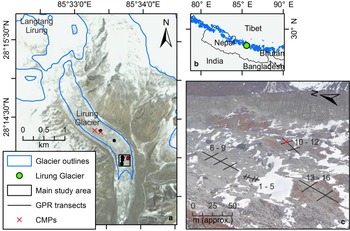
Lirung Glacier is a temperate, largely avalanche-fed valley glacier in the Nepal Himalaya (Fig. 1a), with a total area of 6.3 km2 and a debris-covered area of 1.7 km2. The debris-covered area spans 4000–5300 m elevation and is dominated by a detached, debris-covered tongue, which has a low surface gradient of <10° (Pellicciotti and others, Reference Pellicciotti2015). The tongue is largely stagnant (Kraaijenbrink and others, Reference Kraaijenbrink2016) and has a highly heterogeneous, locally complex topography that supports numerous supraglacial ponds and ice cliffs (Sakai and others, Reference Sakai, Takeuchi, Fujita and Nakawo2000; Steiner and others, Reference Steiner2015; Miles and others, Reference Miles2016). Gades and others (Reference Gades, Conway, Nereson, Naito and Kadota2000) report a debris thickness range of ~0.5 m on the upper ablation zone to ~3 m near the terminus. Lirung Glacier debris is predominantly granitic (Reddy and others, Reference Reddy, Searle and Massey1993) and has a particle size range of <0.001 to >5 m.
(a) Map of Lirung Glacier on DigitalGlobe imagery. (b) Map of Lirung Glacier in the context of country borders and Himalayan glaciers. Glacier outlines are modified from RGI version 5.0. (c) Field photograph of the main study area, showing GPR transect locations in the context of snow cover and heterogeneous topography.

3. METHODS
3.1. Data collection
Fieldwork was carried out in March and April 2015. We collected GPR data using a Sensors and Software pulseEKKO 1000, with 225, 450, 900 and 1200 MHz antennas, varying the operating frequency until the ice surface had been successfully imaged (on the basis that attenuation and range resolution typically decrease with decreasing operating frequency; Davis and Annan, Reference Davis and Annan1989). We collected 29 reflection profiles along 15 transects near the terminus (Fig. 1c) and carried out nine CMPs according to the method outlined by Jol and Bristow (Reference Jol and Bristow2003). Operating frequency and acquisition parameters are presented in Table 1. The 15 transects crossed each other in 11 places, giving 11 tie points and were limited in length and location by patches of wet snow. We used step sizes recommended by the manufacturer (Sensors and Software, 1999), 64-fold stacking and varied the digitisation interval (sample rate) and time window depending on operating frequency and expected debris thickness (Table 1). To ensure good ground coupling and to allow measurements at individual traces to be compared with pit measurements, we collected both reflection profiles and CMPs in ‘step-mode’. We located the GPR transects at 0.25 m intervals using differential global positioning system (DGPS), achieving 0.2 m vertical accuracy and 0.1 m horizontal accuracy. To validate our GPR measurements of debris thickness, we dug 34 pits, ranging from 0.16 to 0.58 m deep, through the debris to the ice surface, along seven of the transects.
GPR data used in this study

Survey type notation is RP, reflection profile; ST, static test; CMP, common midpoint.
3.2. Data quality
Data quality was found to be largely dependent on the acquisition parameters (particularly operating frequency) used during data collection (see Section 5). Poor quality reflection profiles, collected using inappropriate acquisition parameters, were ultimately discarded, and Table 1 shows, which reflection profiles were used to generate debris thickness data. We checked reflection profiles for artefacts and noise, noting that direct waves were slightly misaligned from trace to trace prior to processing, probably due to variable ground coupling. By fitting a straight line of gradient 0.3 m ns−1 to direct waves in CMP plots we found, as expected, that first breaks represent the arrival of the air wave.
3.3. Processing
Reflection profiles were processed using REFLEXW (Sandmeier Software) according to the following steps (after Cassidy, Reference Cassidy and Jolt2009): trace editing, plateau declipping, DC shift, align first breaks at TWTT = 0, dewow, align first breaks at TWTT = antenna separation/speed of light (timezero correction), background removal, bandpass filter, gain correction. Dewow was applied after aligning first breaks at TWTT = 0 because it causes a zero phase filter precursor if applied before (Sensors and Software, 1999) and the dewow time window was set to the same length as the period of the signal of each operating frequency: 4.44, 2.22, 1.11 and 0.83 ns, for 225, 450, 900 and 1200 MHz antennas, respectively. For the bandpass filter, lower cut-off, lower plateau, higher plateau and higher cut-off were set to 0.25×, 0.5×, 1.5× and 3× peak returned frequency, respectively, in order that the width of the plateau pass was similar to the bandwidth (Davis and Annan, Reference Davis and Annan1989) and the taper slope was gentle (Bristow and Jol, Reference Bristow and Jol2003). We chose not to apply topographic correction because the amplitude of topographic change is typically much greater than the amplitude of debris thickness change, and this was found to make interpretation of the ice surface more difficult. We chose not to apply typical gain functions because we did not use a topographic correction, and gain amplifies noise as well as features of interest. Instead, we desaturated the top of each reflection profile by applying a linear negative vertical gain from first breaks (−20 dB) to 1.5× the pulse width from first breaks (0 dB). Horizontal gain was applied in some cases to counter variable penetration depth. CMP data were processed similarly to reflection profiles but timezero was found by fitting a straight line (0.3 m ns−1) to the air wave onset, and we applied no background removal or gain correction. All GPR data are presented as ‘trace normalised’ to account for differences in ground coupling.
Processing significantly aided interpretation of the ice surface. In particular, background removal helped to counteract ‘transmitter blanking’ at the top of reflection profiles due to the high-energy direct wave, and bandpass filtering effectively removed high frequency noise. We note that our choice of dewow time window was possibly not optimal, because the period of the received signal is often different from that of the transmitted signal, and that using a longer time window may have yielded better results.
3.4. Picking
First break picks were made using the REFLEXW ‘autopick’ function, with an amplitude threshold of 0.2, and autocorrected back in time to zero amplitude. We picked first breaks after applying the DC shift filter in order that they were not affected by DC bias.
We picked the ice surface manually at the onset of the first continuous high-amplitude reflection at depth (i.e. the first reflection below the direct wave reflection) in each reflection profile (Fig. 2). Picking was carried out blind, without reference to pit measurements, to avoid interpreter bias. We corrected ice surface picks to zero amplitude using the REFLEXW ‘autocorrect’ function and extracted their positions as TWTTs. In each reflection profile, the debris layer manifests as a high-scatter radar facies and the ice below manifests as a low-scatter radar facies (see Section 4). We used this contrast as a quality check on picks of the ice surface.
An idealised trace through a debris layer, showing first break and ice surface onset picks in relation to timezero. Debris is to the left of the ice surface onset and ice is to the right.

3.5. Wave speed analysis
We calculated debris wave speeds from CMPs by way of coherence analysis and backshifting (after Booth and others, Reference Booth, Clark and Murray2010). Coherence analysis, which is similar to semblance analysis but uses a time window of the same length as the digitisation interval, facilitates assessment of the coherence of reflected waveforms across each CMP and therefore allowed the waveform associated with the ice surface to be picked confidently. Backshifting was necessary because GPR-derived depth measurements require root-mean-square wave speed rather than stacking wave speed, as given by coherence analyses, especially for short-spread conditions, where antenna separation exceeds the depth of the reflector (Booth and others, Reference Booth, Clark and Murray2010).
First, ice surface waveform half-cycles were picked from coherence plots (calculated in REFLEXW) using corresponding reflection profiles as a guide (Fig. 3, left panel). These picks provided zero-offset TWTT t 0 and stacking wave speed v s. Second, t 0 and v s were substituted, with values of antenna separation a, into the normal moveout (NMO) equation (Yilmaz, Reference Yilmaz2001), to define ice surface waveform half-cycle hyperbolas:
 $$t_{\rm a} = \left( {t_0^2 + \; \displaystyle{{a^2} \over {v_{\rm s}^2}}} \right)^{\textstyle\hskip-2pt{1 \over 2}} $$
where t a is the TWTT at some antenna separation or ‘offset’. Third, a chosen hyperbola of each CMP was backshifted, according to the method outlined by Booth and others (Reference Booth, Clark and Murray2010), by ∆t:
 $$\Delta t = \; \displaystyle{T \over 4} + \; \displaystyle{{\left( {HC_n - 1} \right)T} \over 2}$$
where T is the period of the waveform and HC n is the index number of a chosen half-cycle. Lastly, debris wave speed v was calculated from backshifted hyperbolas by rearranging the NMO equation and substituting in new values of t 0 and t a (Yilmaz, Reference Yilmaz2001):
 $$v = \; \left( {\displaystyle{{a^2} \over {t_{\rm a} ^2 - t_0 ^2}}} \right)^{\textstyle\hskip-1pt{1 \over 2}} $$
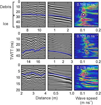
Rows show the results of wave speed analyses performed on each of the three CMPs used to determine debris wave speed. The left-hand column shows the reflection profiles along which CMPs were collected. The middle column shows CMPs. The right-hand column shows coherence analyses. Blue lines represent the ice surface in the left-hand column and backshifted hyperbolas in the middle column. White points represent backshifted wave speeds.

Analysis of three CMPs gave debris wave speeds of 0.107, 0.118 and 0.129 m ns−1 (Fig. 3). Both the mean and median of these three wave speeds is 0.118 m ns−1. This is similar to wave speeds found for other glacial sediments (e.g. 0.12 m ns−1; Degenhardt and others, Reference Degenhardt, Giardino and Junck2003). The remaining six CMPs were not used in wave speed analysis either because a coherent ice surface waveform was not observed or because another CMP taken in the same place with a different operating frequency produced a more coherent reflection.
3.6. Calculating debris thickness
We calculated debris thickness h from ice surface TWTT t, debris wave speed v and antenna separation a, thus taking system geometry into account, according to Eqn (4):
 $$h = \; \displaystyle{1 \over 2}\left(t^2 v^2 - a^2 \right)^{\textstyle\hskip-1pt{1 \over 2}} $$
We used a wave speed of 0.118 m ns−1, which is the mean and median of CMP-derived wave speeds, for all debris thickness calculations and found that correcting for system geometry is important in order to derive realistic debris thickness measurements.
3.7. Uncertainty estimates
We assigned uncertainty to debris thickness measurements by propagating uncertainties assigned to Eq (4) variables (assuming negligible uncertainty associated with a because pulseEKKO 1000 antenna separations are fixed and therefore subject only to manufacturing tolerances), as follows:
 $$\sigma _{\rm h} \approx \; \displaystyle{{vt} \over 2}\left(t^2 v^2 - a^2 \right)^{ - \textstyle{1 \over 2}} \left(v^2 \sigma _{\rm t} + t^2 \sigma _{\rm v} \right)^{\textstyle{1 \over 2}} $$
where σ h is debris thickness uncertainty, σ t is TWTT uncertainty and σ v is wave speed uncertainty.
We attributed σ t to two main sources: (i) misinterpretation of the ice surface due to poor data quality (we assumed the air wave was interpreted well), and (ii) the uncertainty introduced by the digitisation interval on picking first break and ice surface onsets. We assumed that we did not misinterpret the ice surface by more than one period either way (equivalent to λ/2 in terms of thickness or range resolution; cf. Lapazaran and others, Reference Lapazaran, Otero, Martín-Español and Navarro2016) and that ice surface and first break onsets were each picked within 1× the digitisation interval. Because these two sources of uncertainty could occur in the same instance and in the same direction, σ t was calculated as:
 $$\sigma _{\rm t} = \; T + 2D$$
where D is the digitisation interval.
We attributed σ v to the inhomogeneity (variable electromagnetic composition) of the debris, largely controlled by rock type, porosity and pore space filler (water/air/ice); debris wave speed must vary with time and space across the glacier due to variable water content and debris composition. We assumed debris wave speed varied by 10% (after Booth and others, Reference Booth, Clark and Murray2010), which captures the range of wave speeds determined by the three CMPs. Note that this value would have to be much bigger if CMPs were not carried out because the theoretical wave speed range is great. We assumed no covariance between TWTT and wave speed because TWTTs were found using reflection profiles and wave speeds were found by CMP, i.e. by independent means (Pellikka and Rees, Reference Pellikka and Rees2009).
3.8. Reflection power
Reflection power was calculated according to Eqn (7) (following Gades and others, Reference Gades, Conway, Nereson, Naito and Kadota2000; Wilson and others, Reference Wilson, Flowers and Mingo2014):
 $$RP \propto \; \displaystyle{1 \over {(t_2 - t_1 + 1)}}\mathop \sum \limits_{i = t_1} ^{t_2} A_i^2 $$
where RP is reflection power, t 2 and t 1 are the sample numbers that define the time window being analysed, and A is sample amplitude. We used a time window of 1.5T from the ice surface onset.
4. RESULTS
4.1. Ice surface reflection
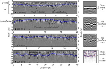
A strong, continuous reflection occurs below the direct wave in 16 of the 29 reflection profiles collected during the main study period (Table 1). Above this reflection is a high-scatter radar facies and below it is a low-scatter radar facies. We interpret strong, continuous reflections as the ice surface (see Section 3.4), and we interpret high- and low-scatter radar facies as debris and ice, respectively (Fig. 4). Four reflection profiles showing a strong continuous reflection at the ice surface, each collected using a different operating frequency, are presented in Figure 4. Ice surface reflection power varies with distance along each reflection profile (e.g. 0.03 – Fig. 4a: weak reflection; 0.39 – Fig. 4a: strong reflection), and reflection power within the debris is typically high (e.g. 0.24 – Fig. 4d: Box i) while reflection power within the ice is typically low (e.g. 0.04 – Fig. 4d: Box ii). The polarity of the ice surface reflection is predominantly − + −, although it is sometimes reversed to + − +. Before processing, the direct wave was seen in all reflection profiles as a continuous, high amplitude, − + − reflection.
Left: ice surface reflection picks (blue) on example reflection profiles in which the ice surface was successfully imaged. (a) T13, 1200 MHz. (b) P1, 900 MHz. (c) P20, 450 MHz. (d) P27, 225 MHz. Depth scales do not take system geometry into account and are therefore approximate. Right: direct wave and ice surface wavelets and the radar facies of debris and ice.

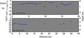
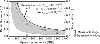
In 13 of the 29 reflection profiles, a strong, continuous reflection is not evident (Table 1). Strong reflections occur in parts of these reflection profiles but show little continuity (e.g. Fig. 5). In places there are strong reflections at multiple depths, and some reflection profiles are dominated by noise – particularly reflection profile P8, which was collected using an operating frequency of 1200 MHz. For reflection profiles collected using each operating frequency, Table 2 shows the minimum, maximum, mean and uncertainties of all debris thickness measurements made and thus describes the measurable debris thickness range of each operating frequency. Using all four operating frequencies (225–1200 MHz), debris thickness measurements range from 0.08 ± 0.29 to 2.30 ± 0.39 m. We typically only observe a strong ice surface reflection through thick debris if a low operating frequency was used and through thin debris if a high operating frequency was used. Therefore penetration depth, measurable debris thickness range and uncertainties (ranging from 0.07 to 0.39 m) are each great for low operating frequencies and small for high operating frequencies. This is shown graphically in Figure 6.
Reflection profiles in which the ice surface was not successfully imaged. Sections of strong ice surface reflection are marked by blue lines. (a) P8, 1200 MHz. (b) P24, 450 MHz. Depth scales do not take system geometry into account and are therefore approximate.

Plot of penetration depth, measurable debris thickness range, and mean uncertainty against operating frequency. The shaded region represents measurable debris thickness range.


4.2. Pit measurements and tie points
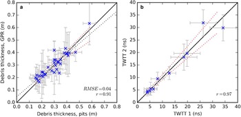
Debris thickness measurements made by GPR agree well with those made by digging pits to the ice surface (Fig. 7a); RMSE = 0.04 m and correlation coefficient r = 0.91. The 1:1 line lies within the 95% confidence interval of linear regression (total least squares) and hypothesis testing for slope of linear regression = 1 gives a P-value of 0.11. Pit measurements are assigned an uncertainty of ±0.05 m. The slope of linear regression (ordinary least squares) through GPR path length vs TWTT, using the same data, gives an independent debris wave speed estimate of 0.110 m ns−1.
(a) Comparison of GPR and pit measurements of debris thickness, where uncertainties on pit measurements are ± 0.05 m. (b) Comparison of TWTTs at tie points. The solid black lines are 1:1 lines, the dotted black lines are total least-squares linear regressions, and the dotted red lines are 95% confidence intervals.

There are 11 tie points at which transects crossed each other. At these tie points, debris thickness and therefore TWTT should be the same, allowing an independent test of wave speed variability. In this study, wave speed may have varied slightly due to variable debris water content in accordance with variable weather conditions. However, there is generally good agreement between tie point picks, as shown in Figure 7b; correlation coefficient r = 0.97 and the 1:1 line lies within the 95% confidence interval of linear regression (total least squares). Hypothesis testing for slope of linear regression = 1 gives a P-value of 0.60. The maximum tie point TWTT pick is 34.0 ns (~1.8 m), and the minimum is 3.9 ns (~0.2 m). The uncertainty bars of all points are plotted here using σ t only.
4.3. Debris thickness and topography
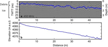
Using each transect only once (where two operating frequencies were used along the same transect, data from the reflection profile with the strongest ice surface reflection were used) and after downsampling all reflection profiles to 0.1 m step size, the mean of GPR debris thickness measurements (n = 3558, from 6199 before downsampling) is 0.84 m and debris thickness ranges from 0.11 ± 0.23 to 2.30 ± 0.39 m. A probability density function (PDF) of debris thickness is presented in Figure 8. Data appear to fit a bimodal distribution with a positive skew towards thinner debris. Debris thickness is highly spatially variable, with a coefficient of variation of 56%. Figure 9 compares debris thickness and topography for a reflection profile collected on the south-facing slope of a hummock. From the top to the bottom of this slope, over a distance of 44.35 m, debris thickness increases from a minimum of 0.11 ± 0.23 to a maximum of 0.83 ± 0.18 m. Debris thickness data (geolocated, before downsampling) are provided in Supplementary Information (also see Table 1).
A probability density function of debris thickness measurements after downsampling (n = 3558).

Comparison of (a) reflection profile P18, 450 MHz, where the blue line represents ice surface reflection picks and (b) DGPS measurements of elevation along P18, recorded every 0.25 m. The depth scale of (a) does not take system geometry into account and is therefore approximate.

5. DISCUSSION
Our results confirm that GPR is a useful tool for mapping debris thickness on Himalayan glaciers and provide an insight into debris thickness variability and the nature of the ice surface during the survey period on Lirung Glacier.
5.1. Ice surface reflection
For each transect, at least one operating frequency produced a reflection profile showing a strong, continuous ice surface reflection. This shows that GPR can be used to image the ice surface through a debris layer, even at shallow depths of <1 m (cf. Lønne and Lauritsen, Reference Lønne and Lauritsen1996; Moorman and Michel, Reference Moorman and Michel2000; Wu and Liu, Reference Wu and Liu2012). Measurable debris thickness ranges reported in Table 2 and Figure 6 indicate that choice of operating frequency is crucial to this end. Where the chosen operating frequency was too high, attenuation prevented detection of the ice surface, e.g. Figure 5b (cf. Annan, Reference Annan and Jol2009). Where the chosen operating frequency was too low, the ice surface reflection is ambiguous because it occurs in the high-energy direct wave (which is usually wider at lower operating frequencies). This has been referred to as ‘transmitter blanking’ (Annan, Reference Annan and Jol2009). Regression through h max (Fig. 6) suggests penetration depth is approximately proportional to f− 0.9, where f is operating frequency, as described by Cook (Reference Cook1975). h min plots on the line h = v/f, where v is median debris wave speed 0.118 m ns−1, suggesting transmitter blanking is typically limited to one wavelength below the debris surface. Measurable debris thickness range is wide for low operating frequencies and narrow for high operating frequencies, and uncertainty increases (largely because range resolution decreases) with decreasing operating frequency. This means a three-way trade-off exists between penetration depth, measurable debris thickness range and uncertainty (cf. Davis and Annan, Reference Davis and Annan1989). If the wavelength of the GPR signal is similar to debris grain size, scattering is likely to inhibit interpretation of the ice surface, as is shown in Figure 5a.
Reflection strength is a function of the difference in relative permittivity (and therefore wave speed) of the materials either side of a reflector, where a large difference in relative permittivity results in a strong reflection (Reynolds, Reference Reynolds2011). Reflection strength is also controlled by the attenuation of the signal as it travels to and from the reflector. As such, the variable strength of the ice surface reflection observed in some reflection profiles could represent lateral changes in:
(1) debris composition, which would cause changes in both the relative permittivity contrast at the ice surface (e.g. due to a change from wet to dry debris or vice versa) and the rate of attenuation in the debris (e.g. due to variable clay content or large point-scatterers); or
(2) ice surface properties (e.g. melt water, emerging englacial debris, or frozen debris on the ice surface, as opposed to a sharp debris/ice interface), which would also cause changes in the relative permittivity contrast at the ice surface.
In particular, a high debris clay or water content should result in a weaker ice surface reflection due to increased attenuation, while a layer of meltwater at the ice surface should give a stronger reflection due to an increased relative permittivity contrast. Despite the variable strength of the ice surface reflection in some reflection profiles, it can often be interpreted confidently due to its continuity.
The continuity of the reflection from any non-horizontal subsurface reflector is largely determined by step size, where small steps give a more continuous reflection than large steps (Jol and Bristow, Reference Jol and Bristow2003). Our data were collected in ‘step-mode’ in order that individual traces could be matched to pit measurements of debris thickness. The step size we used was generally small enough to result in a continuous ice surface reflection. However, a high-resolution, ‘continuous-mode’ survey would likely yield greater continuity still. Penetration depth was limited throughout the study, likely because the debris had high water and clay content. We note that the thickest debris we encountered was 2.30 ± 0.39 m and produced a strong reflection at 225 MHz frequency. Debris and ice are apparent in all reflection profiles as distinctly different radar facies, where debris is seen as a high-scatter radar facies and ice is seen as a low-scatter radar facies. This is likely due largely to the different electromagnetic properties of the different materials (debris comprises heterogeneous point-scatterers while ice is relatively homogenous) and was helpful with regard to interpreting the ice surface.
The polarity of a reflection depends on the sign of its relative permittivity contrast relative to the sign of the previous reflector's relative permittivity contrast, with the sign being negative if relative permittivity contrast is high to low and positive if low to high. If the sign is the same as that of the previous reflector, the polarity of the previous reflection is conserved. If the sign is opposite, the polarity of the previous reflection is reversed (Arcone and others, Reference Arcone, Lawson and Delaney1995). In this study, where the direct wave is − + − and represents the passage of the signal from air to debris (a low to high, positive sign, permittivity contrast) we expect the polarity of the reflection due to the passage of the signal from debris to ice (a high to low, negative sign, permittivity contrast) to be reversed, i.e. + − +. Instead we see the ice surface reflection as a − + −, which indicates the existence of a layer of a high permittivity material at the ice surface.
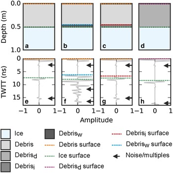
To understand why observed ice surface polarity is different from expected, we modelled the ice surface response to a synthetic, 900 MHz GPR signal (kuepper wavelet) under four sets of theoretical subsurface conditions (Fig. 10):
(1) 0.01 m air over 0.49 m dry debris over ice,
(2) 0.01 m air over 0.44 m dry debris over 0.05 m wet debris over ice,
(3) 0.01 m air over 0.44 m dry debris over 0.05 m icy debris over ice, and
(4) 0.01 m air over 0.49 m damp debris over ice,
using the REFLEXW ‘modelling’ module. We calculated the bulk relative permittivity of layers of dry, damp, wet and icy debris, using Eqn (7) (the Complex Refractive Index Model; Roth and others, Reference Roth, Schulin, Flühler and Attinger1990):
 $$\varepsilon _{\rm b} = (\theta _{{\rm w},i} \varepsilon _{{\rm w},\; i}^\alpha + (1 - \; \eta )\varepsilon _{\rm r}^\alpha + (\eta - \; \theta _{{\rm w},i} )\varepsilon _{\rm a}^\alpha )^{\textstyle{1\over \alpha}} $$
where ε b is bulk relative permittivity and the relative permittivities of air, water, ice and rock are ε a, ε w, ε i and ε r, respectively. η is porosity, as a volume fraction of the debris and α is the orientation of the electrical field induced by the transmitted signal, with respect to the internal geometry of the debris. Water or ice content as a volume fraction of the debris is θ. We used typical relative permittivity values of ε a = 1, ε w = 81 and ε i = 3.2, after Reynolds (Reference Reynolds2011). We assumed a permittivity of 6.5 for ε r, given that Lirung Glacier debris is granitic (Reddy and others, Reference Reddy, Searle and Massey1993) and a debris porosity of 0.3 (Conway and Rasmussen, Reference Conway and Rasmussen2000). We assumed the debris is isotropic, so α is 0.5 (Alharthi and Lange, Reference Alharthi and Lange1987). We assumed low-loss conditions, i.e. there is no attenuation and specify that the pore spaces of wet and dry debris are saturated with water and ice, respectively. Damp debris pore space comprised 20% water and 80% air.
Top row: schematic of four modelled sets of subsurface conditions: (a) 0.01 m air over 0.49 m dry debris over ice. (b) 0.01 m air over 0.44 m dry debris over 0.05 m wet debris over ice. (c) 0.01 m air over 0.44 m dry debris over 0.05 m icy debris over ice. (d) 0.01 m air over 0.49 m damp debris over ice. Bottom row: modelled GPR traces, where (e) corresponds with (a), etc.

Modelled ice surface reflections shown in Figures 10b, c (dry debris over wet debris over ice and dry debris over icy debris over ice) show a − + − sign reflection, similar to what we observe in reflection profiles. This could suggest that the ice surface was typically melting during the survey period or was wet from percolating snowmelt. Alternatively, we might expect that the ice surface was not melting but that there was typically a layer of icy debris above the ice surface, maybe due to a high englacial debris content or the existence of a layer of refrozen meltwater at the ice surface. Both melt water and refrozen meltwater were observed at the ice surface while digging pits.
5.2. Pit measurements and tie points
We were able to dig pits through 0.16–0.58 ± 0.05 m of debris to the ice surface. Digging to greater depths was not possible due to time and labour constraints, so our pit measurements are biased towards shallower depths. Pit measurements of debris thickness show a good fit to GPR measurements of debris thickness (Fig. 7a) and the 1:1 line lies within the 95% confidence interval of linear regression. This indicates that the ice surface can be reliably interpreted as distinct from processing artefacts or multiples of the debris surface and that GPR can realistically be used to measure debris thickness accurately at least in the range 0.16–0.58 m (cf. Moorman and Michel, Reference Moorman and Michel2000; Moorman and others, Reference Moorman, Robinson and Burgess2003; Bradford and others, Reference Bradford, McNamara, Bowden and Gooseff2005; Gusmeroli and others, Reference Gusmeroli2015). The spread of data around the 1:1 line likely represents a combination of picking imprecision and spatio-temporal wave speed variability, and outliers on linear regression are assumed to be mispicks of the ice surface, where the reflections picked are artefacts of processing or the physical expression of some other subsurface feature, for example an off-nadir reflector. The calculated correlation coefficient r = 0.91 is similar to that of other GPR method validation studies in similar environments (e.g. Machguth and others, Reference Machguth, Eisen, Paul and Hoelzle2006; r = 0.92), and the good fit of the data suggests that both CMP-derived debris wave speeds and uncertainty estimates are realistic. The wave speed estimate of 0.110 m ns−1, which was calculated from the gradient of linear regression through path length vs TWTT, is similar to CMP-derived wave speeds (within 10% uncertainty), suggesting debris wave speed did not vary much during the main study period, and is also similar to those found for other glacial sediments (e.g. 0.12 m ns−1; Degenhardt and others, Reference Degenhardt, Giardino and Junck2003). It is possible that GPR measurements of debris thickness are offset from pit measurements by sideswipe or due to a layer of wet debris on the ice surface while surveying.
Despite relatively few data points, the close fit of tie points to the 1:1 line (Fig. 7b) indicates consistent interpretation of the ice surface and an absence of processing artefacts or multiples of the debris surface. It suggests that GPR can be used to measure debris thickness precisely, at least in the debris thickness range ~0.2 to ~1.8 m, covered by the tie points. The 1:1 line lies within the 95% confidence interval of linear regression, suggesting the uncertainties assigned to TWTT are appropriate.
5.3. Debris thickness and topography
The debris thickness data presented here (Fig. 8) are thinner than those of Gades and others (Reference Gades, Conway, Nereson, Naito and Kadota2000), who estimated a debris thickness range ~0.5 m below the headwall to ~3 m near the terminus and Ragettli and others (Reference Ragettli2015), who made ground-based observations of debris thickness across a similar area and found that in 93% of cases debris thickness was >0.5 m (here 33% of measurements are <0.5 m). We observe a debris thickness distribution that is bimodal and positively skewed towards thinner debris. The discrepancy between our measurements and those of earlier studies, and the bimodality of the PDF in Figure 8, might partly reflect the limited spatial coverage of our measurements. However, it is likely that the positive skew is real, and we hypothesise that debris thickness would fit a lognormal or Weibull distribution if further measurements were to be made (e.g. Nicholson and Benn, Reference Nicholson and Benn2012; Reid and others, Reference Reid, Carenzo, Pellicciotti and Brock2012).
Rana and others (Reference Rana, Masayoshi, Yutaka, Kubota and Kojima1998) and Tangborn and Rana (Reference Tangborn and Rana2000) showed that maximum sub-debris melt rate on Lirung Glacier occurs where debris is 0.03 m thick and that the critical thickness is 0.08 m. As such, our data show that debris almost as thin as the critical thickness is present near the terminus of Lirung Glacier. From the thickness at which sub-debris melt rate is maximum to ~0.5 m, debris cover has an increasingly insulating effect on melt rate (Nicholson and Benn, Reference Nicholson and Benn2006), so if we classify thin debris as that which is thinner than the critical thickness, thick debris as that which is thicker than 0.5 m, and intermediate debris as that which is between thick and thin, 33% of measurements are intermediate and 67% are thick. On this basis, sub-debris melting, as well as englacial conduit collapse and melting at ice cliffs and ponds (e.g. Basnett and others, Reference Basnett, Kulkarni and Bolch2013; Immerzeel and others, Reference Immerzeel2014; Steiner and others, Reference Steiner2015; Miles and others, Reference Miles2016), is likely important in terms of mass loss on the debris-covered tongue.
For an idealised debris-covered glacier in steady state, with no debris input from avalanches, debris thickness on the ablation zone is controlled by englacial debris content, melt rate and surface velocity (Nakawo and others, Reference Nakawo, Iwata and Yoshida1986) and increases systematically down-glacier (Konrad and Humphrey, Reference Konrad and Humphrey2000). Figure 9 shows that at small scales (of order 10 m) there is likely a link between debris thickness and topography; debris is thinner on the flank than at the base of the hummock, indicating redistribution by slope processes. Because variable debris thickness causes differential melting and differential melting causes variable surface lowering, there is likely a feedback between debris thickness and surface topography (e.g. Nicholson and Benn, Reference Nicholson and Benn2012; Reid and others, Reference Reid, Carenzo, Pellicciotti and Brock2012). We suggest that slope processes are affecting debris thickness variability at a local scale and, in turn, that debris thickness variability is an important control on the surface evolution of the glacier, whereby high debris thickness variability promotes the development of hummocky topography, lakes, and ice cliffs and vice versa. We suggest that variable debris thickness explains some of the highly variable surface lowering observed on the ablation zone of Lirung Glacier by Immerzeel and others (Reference Immerzeel2014) and Pellicciotti and others (Reference Pellicciotti2015).
5.4. Technical issues and recommendations
The highly variable topography and rough surfaces of debris-covered glaciers can make carrying out GPR surveys physically difficult and time consuming. Despite this, GPR offers significant benefits over alternative methods of measuring debris thickness; GPR is much quicker than digging pits, less biased than measuring debris thickness at ice cliffs and allows a wide debris thickness range to be measured at high spatial resolution. Jol and Bristow (Reference Jol and Bristow2003) make general recommendations for a successful GPR survey, many of which were found to be very useful in carrying out this work. With respect to measuring debris thickness, we recommend:
(1) Surveys should be carried out in snow-free conditions to permit a strong ice surface reflection. Long transects should be set up where possible, in order to make the ice surface easier to interpret.
(2) An appropriate multi-frequency GPR could be used to cover most debris thickness eventualities, significantly reducing survey time. Figure 6 can be used as a guide to choosing acquisition parameters. Collecting GPR data in ‘continuous-mode’ would likely result in a clearer reflection at the ice surface in areas where the debris surface is relatively smooth.
(3) GPR should be used with in conjunction with pits or CMPs in order to determine debris wave speed to make realistic debris thickness calculations. Topographic correction using DGPS measurements does not significantly improve ice surface interpretability.
(4) Transmitter blanking limits the use of GPR for measuring the thickness of thin debris (<0.1 m), where pits are more appropriate.
Future work should aim to carry out more extensive GPR surveys on the ablation zones of other debris-covered glaciers in order to better characterise debris thickness variability and to test remote sensing approaches to mapping debris thickness. The relationship between debris thickness and local surface topography should be investigated further.
6. CONCLUSIONS
We test the use of GPR for measuring debris thickness on Lirung Glacier, Nepal, accounting for the geometry of the GPR system and propagating the associated uncertainties. Reflection profiles show a strong, continuous reflection at the ice surface in the debris thickness range tested, provided that appropriate acquisition parameters were used during data collection. GPR measurements of debris thickness correlate well with pit measurements and TWTTs show good agreement at tie points. With respect to acquisition parameters, a three-way trade-off exists between penetration depth, measurable debris thickness range and uncertainty, where high operating frequencies are suitable for thinner debris and low operating frequencies are suitable for thicker debris. Debris wave speed (0.107–0.129 m ns−1) was surprisingly invariable during the survey period, and penetration depth through the debris was limited (max. 2.30 ± 0.39 m at 225 MHz). Debris presents as a high-scatter radar facies while ice presents as low-scatter.
Debris almost as thin as the critical thickness is present near the terminus of Lirung Glacier and debris thickness is highly variable over small spatial scales (of order 10 m), ranging from 0.11 ± 0.23 to 2.30 ± 0.39 m with a coefficient of variation of 56%. 33% of our debris thickness measurements are <0.5 m, which would suggest that sub-debris melting is important on the ablation zone of Lirung Glacier. Debris thickness appears to vary with slope, indicating redistribution by slope processes, and we suggest that variable debris thickness is a cause of variable surface lowering and therefore debris cover redistribution (and debris thickness change) on Lirung Glacier. The polarity of ice surface reflections is commonly − + −, indicating wet or icy debris at the ice surface during the survey period.
We conclude that GPR can be used to measure debris thickness more quickly than digging pits, which are typically limited to thicknesses <1 m, and allows more extensive sampling than surveying debris exposures along ice cliffs. As such, it is a valuable tool with which to map debris thickness distribution. Key limitations are the subjectivity of manual picks of the ice surface, the narrow debris thickness range for which each operating frequency can be used and the typically rough nature of debris-covered glacier surfaces. We find that system geometry is an important consideration if the ice surface is shallow compared with antenna separation and that debris wave speed must be measured (using CMPs or pits) to derive accurate debris thickness measurements. Figure 6 is potentially useful as a guide to choosing appropriate acquisition parameters for a GPR survey of debris thickness and we suggest that future work should use GPR to test or calibrate methods of mapping debris thickness using satellite imagery.
SUPPLEMENTARY MATERIAL
To view supplementary material for this article, please visit https://doi.org/10.1017/jog.2017.18
ACKNOWLEDGEMENTS
We sincerely thank Adam Booth and one anonymous reviewer, whose comments and suggestions helped improve and clarify this manuscript. M.M. is funded by NERC DTP grant number: NE/L002507/1, receives CASE funding from Reynolds International Ltd, and was provided travel support by the Jesus College Doctoral Research Fund. I.W. was funded by the BB Roberts Fund, University Travel Fund and St Catharine's College Research Fund. Equipment (GPR and DGPS) was provided under NERC Geophysical Equipment Facility grant number: 1014.


 Open access