
 φ
φ





1. Introduction
The main focus of this article is to study the structure of Gibbs measures of uniform $M$
-Lipschitz function on regular trees. Our broader goal is to better understand the structure of Gibbs measures for random surface models with hardcore constraints on graphs of hyperbolic flavour. The theory of Bernoulli percolation on such graphs has seen tremendous progress in the past few decades [Reference Benjamini and Schramm4, Reference Lyons and Peres20]. In contrast, the results on other popular statistical physics models like the Ising model on such graphs have been few and far between [Reference Georgii9, Reference Häggström, Schonmann and Steif12–Reference Jonasson and Steif14]. On the other hand, the study of height function models on planar lattices, particularly the structure of Gibbs measures on them, have garnered a lot of attention in recent years [Reference Chandgotia, Peled, Sheffield and Tassy6, Reference Duminil-Copin, Harel, Laslier, Raoufi and Ray7, Reference Lammers and Toninelli18, Reference Peled21]. For finite graphs like expanders and wired regular trees, it is known [Reference Benjamini, Häggström and Mossel1, Reference Galvin8, Reference Peled, Samotij and Yehudayoff22, Reference Peled, Samotij and Yehudayoff23] that the height function models are mostly flat and the height function has a doubly exponential tail. However, finer questions about the existence of local weak limits and its dependence on boundary conditions remain unanswered. Our main focus is to initiate the study of weak local convergence of height functions on regular trees imposing various boundary conditions on the leaves. An even broader goal is to classify all possible extremal Gibbs measures on trees.
$M$
-Lipschitz function on regular trees. Our broader goal is to better understand the structure of Gibbs measures for random surface models with hardcore constraints on graphs of hyperbolic flavour. The theory of Bernoulli percolation on such graphs has seen tremendous progress in the past few decades [Reference Benjamini and Schramm4, Reference Lyons and Peres20]. In contrast, the results on other popular statistical physics models like the Ising model on such graphs have been few and far between [Reference Georgii9, Reference Häggström, Schonmann and Steif12–Reference Jonasson and Steif14]. On the other hand, the study of height function models on planar lattices, particularly the structure of Gibbs measures on them, have garnered a lot of attention in recent years [Reference Chandgotia, Peled, Sheffield and Tassy6, Reference Duminil-Copin, Harel, Laslier, Raoufi and Ray7, Reference Lammers and Toninelli18, Reference Peled21]. For finite graphs like expanders and wired regular trees, it is known [Reference Benjamini, Häggström and Mossel1, Reference Galvin8, Reference Peled, Samotij and Yehudayoff22, Reference Peled, Samotij and Yehudayoff23] that the height function models are mostly flat and the height function has a doubly exponential tail. However, finer questions about the existence of local weak limits and its dependence on boundary conditions remain unanswered. Our main focus is to initiate the study of weak local convergence of height functions on regular trees imposing various boundary conditions on the leaves. An even broader goal is to classify all possible extremal Gibbs measures on trees.
Let us fix some notations before getting into our main results. An $M$
-Lipschitz function on a graph
$M$
-Lipschitz function on a graph $G=(V,E)$
is a function
$G=(V,E)$
is a function $f \colon V \to \mathbb{Z}$
satisfying that
$f \colon V \to \mathbb{Z}$
satisfying that
 \begin{equation*}|\,f(u) - f(v)| \le M\text{ for all }u \sim v,\end{equation*}
where $u \sim v$
means
$u \sim v$
means $u$
is a neighbour of
$u$
is a neighbour of $v$
. If
$v$
. If $M=1$
, we drop the
$M=1$
, we drop the $M$
from the terminology and simply refer to the function as a Lipschitz function. A
$M$
from the terminology and simply refer to the function as a Lipschitz function. A $d$
-ary tree is a connected graph with no cycles such that every vertex has degree
$d$
-ary tree is a connected graph with no cycles such that every vertex has degree $d+1$
except one vertex, called the root vertex, which has degree
$d+1$
except one vertex, called the root vertex, which has degree $d$
. We denote by
$d$
. We denote by $\mathbb T_d$
the
$\mathbb T_d$
the $d$
-ary treeFootnote
1
with the root vertex denoted
$d$
-ary treeFootnote
1
with the root vertex denoted $\rho$
. Let
$\rho$
. Let $\mathbb{T}_d^k$
denote the finite subgraph of
$\mathbb{T}_d^k$
denote the finite subgraph of $\mathbb{T}_d$
induced by the vertices within distance
$\mathbb{T}_d$
induced by the vertices within distance $k$
from
$k$
from $\rho$
. For a finite set
$\rho$
. For a finite set $S \subset \mathbb{Z}$
, let
$S \subset \mathbb{Z}$
, let $\mathcal{L}_{k,d}(S)$
denote the set of Lipschitz functions on
$\mathcal{L}_{k,d}(S)$
denote the set of Lipschitz functions on $\mathbb{T}_d^k$
where the values on the leaves are constrained to be in
$\mathbb{T}_d^k$
where the values on the leaves are constrained to be in $S$
. Let
$S$
. Let $\mu _{k,d}^{S}$
denote the uniform law on
$\mu _{k,d}^{S}$
denote the uniform law on $\mathcal{L}_{k,d}(S)$
. In the special case
$\mathcal{L}_{k,d}(S)$
. In the special case $S= \{0\}$
, which we refer to as zero boundary conditions, we write
$S= \{0\}$
, which we refer to as zero boundary conditions, we write $\mu _{n,d}^0$
and
$\mu _{n,d}^0$
and $\mathcal{L}_{k,d}^0$
for short.
$\mathcal{L}_{k,d}^0$
for short.
The main result in this article is the existence of a transition in the convergence behaviour of random 1-Lipschitz functions under zero boundary conditions.
Theorem 1.1. $\mu ^0_{k,d}$
converges as
$\mu ^0_{k,d}$
converges as $k \to \infty$
if and only if
$k \to \infty$
if and only if $2 \le d \le 7$
.
$2 \le d \le 7$
.
The convergence above is in the local weak sense. Actually, the convergence result for $2 \le d \le 7$
in Theorem1.1 that we prove is more general: it holds for symmetric weighted boundary conditions on the leaves which satisfy a certain decay condition (we call these the good weight sequences in Section 2.3). The result implies in particular that for any
$2 \le d \le 7$
in Theorem1.1 that we prove is more general: it holds for symmetric weighted boundary conditions on the leaves which satisfy a certain decay condition (we call these the good weight sequences in Section 2.3). The result implies in particular that for any $N \ge 1$
, the measures
$N \ge 1$
, the measures $\mu ^{\{-N,\dots ,N\}}_{k,d}$
converge to the same limit as that with zero boundary conditions. See Theorem2.6 for a complete statement of the full result.
$\mu ^{\{-N,\dots ,N\}}_{k,d}$
converge to the same limit as that with zero boundary conditions. See Theorem2.6 for a complete statement of the full result.
In contrast, the next result shows that for other boundary conditions, the above convergence vs. non-convergence phenomenon does not occur.
Theorem 1.2. $\mu ^{\{0,1\}}_{k,d}$
converges as
$\mu ^{\{0,1\}}_{k,d}$
converges as $k \to \infty$
for all
$k \to \infty$
for all $d \ge 2$
.
$d \ge 2$
.
The above theorem is a consequence of a version of an FKG property for the absolute value of the Lipschitz function when shifted by $1/2$
.
$1/2$
.
It is easy to see for any finite $S$
that
$S$
that $\mu _{d}^{S}\,:\!=\,\lim _{k \to \infty }\mu ^S_{k,d}$
, when it exists, is a tree-indexed Markov chain. This follows from the observation that the set of
$\mu _{d}^{S}\,:\!=\,\lim _{k \to \infty }\mu ^S_{k,d}$
, when it exists, is a tree-indexed Markov chain. This follows from the observation that the set of $f \in \mathcal{L}_{k,d}(S)$
with a given value at a given vertex, splits into a Cartesian product over the subtrees rooted at that vertex. Furthermore, it is not hard to check that no such Markov chain (obtained as a limit of
$f \in \mathcal{L}_{k,d}(S)$
with a given value at a given vertex, splits into a Cartesian product over the subtrees rooted at that vertex. Furthermore, it is not hard to check that no such Markov chain (obtained as a limit of $\mu ^S_{k,d}$
) is a non-trivial mixture of other similar Markov chains (simply apply ergodic theorem along a ray). In particular, when
$\mu ^S_{k,d}$
) is a non-trivial mixture of other similar Markov chains (simply apply ergodic theorem along a ray). In particular, when $2 \le d \le 7$
, the limiting measures
$2 \le d \le 7$
, the limiting measures $\{\mu ^{\{i\}}_{d}\}_{i \in \mathbb{Z}}$
obtained in Theorem1.1 and the limiting measures
$\{\mu ^{\{i\}}_{d}\}_{i \in \mathbb{Z}}$
obtained in Theorem1.1 and the limiting measures $\{\mu ^{\{i,i+1\}}_d\}_{i \in \mathbb{Z}}$
obtained in Theorem1.2 are Markov chains, none of which is a mixture of the others.
$\{\mu ^{\{i,i+1\}}_d\}_{i \in \mathbb{Z}}$
obtained in Theorem1.2 are Markov chains, none of which is a mixture of the others.
We also prove a general result which works beyond trees and for general $M$
. Let
$M$
. Let $G$
be an infinite bipartite connected graph with maximum degree
$G$
be an infinite bipartite connected graph with maximum degree $d$
and Cheeger constant
$d$
and Cheeger constant $h$
. Recall that the Cheeger constant of a graph is defined as
$h$
. Recall that the Cheeger constant of a graph is defined as
 \begin{equation*} h=h(G)\,:\!=\,\inf _{S \subset V, 0\lt |S|\lt \infty } \frac {|\partial S|}{|S|}, \end{equation*}
where $\partial S$
is the set of vertices in
$\partial S$
is the set of vertices in $G$
, which are not in
$G$
, which are not in $S$
but have at least one neighbour in
$S$
but have at least one neighbour in $S$
, and
$S$
, and $|\cdot |$
denote the cardinality. We establish the existence of (multiple forms of) long-range order for
$|\cdot |$
denote the cardinality. We establish the existence of (multiple forms of) long-range order for $M$
-Lipschitz functions on
$M$
-Lipschitz functions on $G$
in the regime where
$G$
in the regime where $h \gg M$
. Observe that since trivially
$h \gg M$
. Observe that since trivially $h \le d$
, the condition
$h \le d$
, the condition $h \gg M$
requires that
$h \gg M$
requires that $d \gg M$
. Furthermore, note that a
$d \gg M$
. Furthermore, note that a $d$
-regular tree has Cheeger constant
$d$
-regular tree has Cheeger constant $d-2$
.
$d-2$
.
Colour the partite classes of $G$
black and white. Given a finite set
$G$
black and white. Given a finite set $U$
of
$U$
of $G$
, and finite sets
$G$
, and finite sets $S_\circ ,S_\bullet \subset \mathbb{Z}$
, let
$S_\circ ,S_\bullet \subset \mathbb{Z}$
, let $\mathcal{L}_{U,M}(S_\circ ,S_\bullet )$
denote the set of all
$\mathcal{L}_{U,M}(S_\circ ,S_\bullet )$
denote the set of all $M$
-Lipschitz functions on
$M$
-Lipschitz functions on $U \cup \partial U$
with the values on
$U \cup \partial U$
with the values on $\partial U$
constrained to be in
$\partial U$
constrained to be in $S_\circ$
or
$S_\circ$
or $S_\bullet$
according to their colour. Given integers
$S_\bullet$
according to their colour. Given integers $a \le b$
, let
$a \le b$
, let $\nu ^{a,b}_{U,M}$
denote the uniform measure on
$\nu ^{a,b}_{U,M}$
denote the uniform measure on $\mathcal{L}_{U,M}(S_\circ ,S_\bullet )$
with
$\mathcal{L}_{U,M}(S_\circ ,S_\bullet )$
with $S_\circ =\{a,\dots ,b\},S_\bullet =\{b-M,\dots ,a+M\}$
. The choice of
$S_\circ =\{a,\dots ,b\},S_\bullet =\{b-M,\dots ,a+M\}$
. The choice of $S_\circ ,S_\bullet$
is an artefact of the proof technique: with these boundary conditions, on a graph with large Cheeger constant, a uniform
$S_\circ ,S_\bullet$
is an artefact of the proof technique: with these boundary conditions, on a graph with large Cheeger constant, a uniform $M$
-Lipschitz function behaves approximately like i.i.d. Uniform
$M$
-Lipschitz function behaves approximately like i.i.d. Uniform $(S_\circ )$
on white vertices and i.i.d. uniform
$(S_\circ )$
on white vertices and i.i.d. uniform $(S_\bullet )$
on black vertices. Note that the sets
$(S_\bullet )$
on black vertices. Note that the sets $S_{\circ }$
and
$S_{\circ }$
and $S_{\bullet }$
are complementary in the sense that if for a given vertex our only knowledge about its value is that it belongs to
$S_{\bullet }$
are complementary in the sense that if for a given vertex our only knowledge about its value is that it belongs to $S_{\circ }$
, then the possible values at any of its neighbours is precisely described by
$S_{\circ }$
, then the possible values at any of its neighbours is precisely described by $S_{\bullet }$
, and vice versa. An exhaustion of
$S_{\bullet }$
, and vice versa. An exhaustion of $G$
is a sequence of finite sets increasing to
$G$
is a sequence of finite sets increasing to $G$
, i.e.,
$G$
, i.e., $G_1\subset G_2\subset \cdots$
and
$G_1\subset G_2\subset \cdots$
and $\cup _{i \ge 1} G_i = G$
.
$\cup _{i \ge 1} G_i = G$
.
Theorem 1.3.
Assume that $h \ge 6M\log (3d^4(4M+1))$
. Let
$h \ge 6M\log (3d^4(4M+1))$
. Let $a \le b$
be integers such that
$a \le b$
be integers such that $b-a \le 2M$
.
$b-a \le 2M$
.
-
a. Let $(G_k)$
be an exhaustion. Then
$\nu _{G_k,M}^{a,b}$
converges as
$k\to \infty$
to a Gibbs measure
$\nu _{G,M}^{a,b}$
.
$(G_k)$
be an exhaustion. Then
$\nu _{G_k,M}^{a,b}$
converges as
$k\to \infty$
to a Gibbs measure
$\nu _{G,M}^{a,b}$
. -
b. The measures
$\nu _{G,M}^{a,b}$
are distinct for different pairs
$(a,b)$
.


The limiting measure $\nu _{G,M}^{a,b}$
is necessarily independent of the chosen exhaustion (as one can interleave two exhaustions and then apply the result). Observe that the pushforward of
$\nu _{G,M}^{a,b}$
is necessarily independent of the chosen exhaustion (as one can interleave two exhaustions and then apply the result). Observe that the pushforward of $\nu _{U,M}^{a,b}$
by a parity-preserving automorphism
$\nu _{U,M}^{a,b}$
by a parity-preserving automorphism $\varphi$
of
$\varphi$
of $G$
is
$G$
is $\nu _{\varphi (U),M}^{a,b}$
. It follows that the limiting measure
$\nu _{\varphi (U),M}^{a,b}$
. It follows that the limiting measure $\nu _{G,M}^{a,b}$
is invariant to parity-preserving automorphisms of
$\nu _{G,M}^{a,b}$
is invariant to parity-preserving automorphisms of $G$
. Similarly, the pushforward of
$G$
. Similarly, the pushforward of $\nu _{G,M}^{a,b}$
by a parity-reversing automorphism is
$\nu _{G,M}^{a,b}$
by a parity-reversing automorphism is $\nu _{G,M}^{b-M,a+M}$
. Thus,
$\nu _{G,M}^{b-M,a+M}$
. Thus, $\nu _{G,M}^{a,b}$
is invariant to all automorphisms if and only if
$\nu _{G,M}^{a,b}$
is invariant to all automorphisms if and only if $b-a=M$
. Consequently, when
$b-a=M$
. Consequently, when $b-a \neq M$
, the measure
$b-a \neq M$
, the measure $\nu _{G,M}^{a,b}$
behaves differently on even and odd vertices. In fact, the height on any even vertex is close to uniform on
$\nu _{G,M}^{a,b}$
behaves differently on even and odd vertices. In fact, the height on any even vertex is close to uniform on $\{a,\dots ,b\}$
, and the height on any odd vertex is close to uniform on
$\{a,\dots ,b\}$
, and the height on any odd vertex is close to uniform on $\{b-M,\dots ,a+M\}$
(see Proposition3.1). Thus, Theorem1.3 gives a separate proof of the non-convergence result in Theorem1.1 when
$\{b-M,\dots ,a+M\}$
(see Proposition3.1). Thus, Theorem1.3 gives a separate proof of the non-convergence result in Theorem1.1 when $d$
is large enough. Let us also remark that in the case when
$d$
is large enough. Let us also remark that in the case when $b-a=M$
, the result stated in the theorem makes sense and holds true even without the assumption that the graph
$b-a=M$
, the result stated in the theorem makes sense and holds true even without the assumption that the graph $G$
is bipartite (in this case
$G$
is bipartite (in this case $\nu ^{a,b}_{U,M}$
is the uniform measure on
$\nu ^{a,b}_{U,M}$
is the uniform measure on $M$
-Lipschitz functions constrained to taking values in
$M$
-Lipschitz functions constrained to taking values in $\{a,\dots ,b\}$
on the entire boundary).
$\{a,\dots ,b\}$
on the entire boundary).
Background: Studying Gibbs measures of statistical physics models on trees has a long history. We refer to the book of Rozikov [Reference Rozikov25] for a comprehensive survey of the results about splitting Gibbs measures on regular trees for models with countable and even uncountable spin values. It is interesting to note that the results in [Reference Rozikov25] about splitting Gibbs measure for countable spins (see [Reference Rozikov25, Theorem 8.1]) lead to a unique Gibbs measure. This is clearly not the case for us, as Theorem1.1 (see also Theorem2.6) already leads to multiple solutions, and it is plausible that there are many more (see Section 5).
The random homomorphism model is very similar to the uniform Lipschitz model, except that the height difference between adjacent vertices must be in $\{\pm 1\}$
(this makes sense only on bipartite graphs). Both the uniform Lipschitz model and the random homomorphism model on trees have been studied in [Reference Benjamini, Häggström and Mossel1, Reference Peled, Samotij and Yehudayoff22] and on finite expanders in [Reference Peled, Samotij and Yehudayoff23]. A recent paper by Lammers and Toninelli [Reference Lammers and Toninelli18] exploits log concavity to obtain localization for homomorphisms with very general boundary conditions. See also a recent result by Krueger, Li, and Park [Reference Krueger, Li and Park17], which significantly improves the results in [Reference Peled, Samotij and Yehudayoff23]. See [Reference Kissel, Külske and Rozikov16] for a result about the Widom–Rowlinson model on trees, which is a model of similar flavour to ours (it can be thought of as a restricted Lipschitz model where the function cannot take values other than
$\{\pm 1\}$
(this makes sense only on bipartite graphs). Both the uniform Lipschitz model and the random homomorphism model on trees have been studied in [Reference Benjamini, Häggström and Mossel1, Reference Peled, Samotij and Yehudayoff22] and on finite expanders in [Reference Peled, Samotij and Yehudayoff23]. A recent paper by Lammers and Toninelli [Reference Lammers and Toninelli18] exploits log concavity to obtain localization for homomorphisms with very general boundary conditions. See also a recent result by Krueger, Li, and Park [Reference Krueger, Li and Park17], which significantly improves the results in [Reference Peled, Samotij and Yehudayoff23]. See [Reference Kissel, Külske and Rozikov16] for a result about the Widom–Rowlinson model on trees, which is a model of similar flavour to ours (it can be thought of as a restricted Lipschitz model where the function cannot take values other than $\{-1,0,1\}$
). See Peled and Spinka [Reference Peled21, Reference Peled and Spinka24] for analogous results in the hypercubic lattice. See also [Reference Benjamini and Peres2, Reference Benjamini and Schechtman3, Reference Benjamini, Yadin and Yehudayoff5] for related results.
$\{-1,0,1\}$
). See Peled and Spinka [Reference Peled21, Reference Peled and Spinka24] for analogous results in the hypercubic lattice. See also [Reference Benjamini and Peres2, Reference Benjamini and Schechtman3, Reference Benjamini, Yadin and Yehudayoff5] for related results.
As mentioned, the fact that random Lipschitz functions on trees under zero boundary conditions are localized was first proved by Peled, Samotij, and Yehudayoff [Reference Peled, Samotij and Yehudayoff22]. In fact, they showed that the height at the root has doubly exponential tails for all $M \ge 1$
and
$M \ge 1$
and $d \ge 2$
. They also point outFootnote
2
that when
$d \ge 2$
. They also point outFootnote
2
that when $M \le cd/\log d$
for some universal constant
$M \le cd/\log d$
for some universal constant $c\gt 0$
, more is true – for even
$c\gt 0$
, more is true – for even $n$
, the height at the root is exponentially concentrated on the single value
$n$
, the height at the root is exponentially concentrated on the single value $0$
, whereas for odd
$0$
, whereas for odd $n$
, the height at the root is roughly uniformly distributed on
$n$
, the height at the root is roughly uniformly distributed on $\{-M,\dots ,M\}$
. They go on to explain that they expect that such a strong concentration fails when
$\{-M,\dots ,M\}$
. They go on to explain that they expect that such a strong concentration fails when $M\gg d$
. Specifically, they raised their suspicion that the height at the root converges in distribution as
$M\gg d$
. Specifically, they raised their suspicion that the height at the root converges in distribution as $n$
tends to infinity (so that there is asymptotically no distinction between even and odd tree heights). While we do not establish that such a transition phenomenon occurs between the cases
$n$
tends to infinity (so that there is asymptotically no distinction between even and odd tree heights). While we do not establish that such a transition phenomenon occurs between the cases $M\ll d$
and
$M\ll d$
and $M \gg d$
for all
$M \gg d$
for all $M$
, we do show in Theorem1.1 that such a transition occurs as
$M$
, we do show in Theorem1.1 that such a transition occurs as $d$
is varied when
$d$
is varied when $M=1$
. Extending this to all
$M=1$
. Extending this to all $M$
is an interesting problem.
$M$
is an interesting problem.
Proof outline: Let us briefly outline the ideas behind the proofs. Theorem1.1 is the major result in this article and takes up most of the analysis. There are two separate parts, convergence for $2 \le d \le 7$
and non-convergence for
$2 \le d \le 7$
and non-convergence for $d \ge 8$
, the latter being much simpler. The basic idea for the convergence part is a contraction argument: we think of the probability distribution at the root as an element of
$d \ge 8$
, the latter being much simpler. The basic idea for the convergence part is a contraction argument: we think of the probability distribution at the root as an element of $\ell ^1(\mathbb{Z})$
, and then we apply iterates of an appropriate operator
$\ell ^1(\mathbb{Z})$
, and then we apply iterates of an appropriate operator $F$
. The goal then reduces to proving that the iterates of
$F$
. The goal then reduces to proving that the iterates of $F$
(applied to
$F$
(applied to $\delta _0$
, i.e., the probability measure assigning unit mass to
$\delta _0$
, i.e., the probability measure assigning unit mass to $0$
) converge in an appropriate norm. The proof of this would have been somewhat straightforward if the map
$0$
) converge in an appropriate norm. The proof of this would have been somewhat straightforward if the map $F$
turned out to be a contraction (but it isn’t). Nevertheless, we show that after a number of iterations, we get into a certain ‘basin of attraction’, on which the map becomes a contraction. To show the latter, we prove that the operator norm of the derivative of
$F$
turned out to be a contraction (but it isn’t). Nevertheless, we show that after a number of iterations, we get into a certain ‘basin of attraction’, on which the map becomes a contraction. To show the latter, we prove that the operator norm of the derivative of $F$
is strictly less than 1 in this basin. After this, the proof concludes by a simple application of the Banach fixed point theorem.
$F$
is strictly less than 1 in this basin. After this, the proof concludes by a simple application of the Banach fixed point theorem.
In practice, directly applying this idea to $F$
soon becomes intractable. The way we work our way through is to look at ratios of the consecutive values, which gets rid of the normalizing factor in a good way. For the non-convergence part of the theorem, we show that the iterates oscillate between two separated ‘basins’, ruling out the possibility of convergence (though we still expect convergence of
$F$
soon becomes intractable. The way we work our way through is to look at ratios of the consecutive values, which gets rid of the normalizing factor in a good way. For the non-convergence part of the theorem, we show that the iterates oscillate between two separated ‘basins’, ruling out the possibility of convergence (though we still expect convergence of $\mu ^0_{k,d}$
along even
$\mu ^0_{k,d}$
along even $k$
). The details of these ideas can be found in Section 2.
$k$
). The details of these ideas can be found in Section 2.
Theorem1.2 follows from a certain ‘FKG for absolute value’ result when the height function is shifted by $1/2$
. Finally, Theorem1.3 is a consequence of a variation of a Peierl’s type argument following that in [Reference Peled, Samotij and Yehudayoff22, Reference Peled, Samotij and Yehudayoff23].
$1/2$
. Finally, Theorem1.3 is a consequence of a variation of a Peierl’s type argument following that in [Reference Peled, Samotij and Yehudayoff22, Reference Peled, Samotij and Yehudayoff23].
Organization: In Section 2, we describe the setup and the ratio transformation which simplifies the operator $F$
. We also describe heuristically which observables from this operator drives the transition from convergence to non-convergence. In Section 2.1 we define the set which is the ‘basin of attraction’ and describe our procedure to get into this set. In Section 2.2, we prove the non-convergence part of Theorem1.1. In Sections 2.3–2.5 we prove the convergence part of Theorem1.1 modulo some technical estimates, which we push to Section 6. We prove Theorem1.2 in Section 4 and Theorem1.3 in Section 3. We list some open questions in Section 5.
$F$
. We also describe heuristically which observables from this operator drives the transition from convergence to non-convergence. In Section 2.1 we define the set which is the ‘basin of attraction’ and describe our procedure to get into this set. In Section 2.2, we prove the non-convergence part of Theorem1.1. In Sections 2.3–2.5 we prove the convergence part of Theorem1.1 modulo some technical estimates, which we push to Section 6. We prove Theorem1.2 in Section 4 and Theorem1.3 in Section 3. We list some open questions in Section 5.
2. Convergence and non-convergence under 0 boundary conditions
In this section, we prove Theorem1.1. The proof is separated into the convergence result for $2 \le d \le 7$
(Section 2.3) and the non-convergence result for
$2 \le d \le 7$
(Section 2.3) and the non-convergence result for $d \ge 8$
(Section 2.2). The proofs are based on a recursive approach. We now lay the groundwork for this.
$d \ge 8$
(Section 2.2). The proofs are based on a recursive approach. We now lay the groundwork for this.
For a probability distribution $z=(z_i)_{i \in \mathbb{Z}}$
, define
$z=(z_i)_{i \in \mathbb{Z}}$
, define
 \begin{align*} A(z)_i \,:\!=\, \left (z_{i-1}+z_i+z_{i+1}\right )^d , \qquad F(z) \,:\!=\, \frac {A(z)}{\sum _{i \in \mathbb{Z}} A(z)_i}. \end{align*}
The particular form of $A(z)$
arises from the Lipschitz condition, while
$A(z)$
arises from the Lipschitz condition, while $F(z)$
is just a normalization of
$F(z)$
is just a normalization of $A(z)$
. We write
$A(z)$
. We write $F^{(k)}$
for the
$F^{(k)}$
for the $k$
-fold composition of
$k$
-fold composition of $F$
, i.e.,
$F$
, i.e., $F^{(0)}$
is the identity and
$F^{(0)}$
is the identity and $F^{(k+1)}=F \circ F^{(k)}$
.
$F^{(k+1)}=F \circ F^{(k)}$
.
Claim 2.1.
Let $f_k \sim \mu _{k,d}^0$
, and let
$f_k \sim \mu _{k,d}^0$
, and let $\rho$
be the root vertex. Then for any
$\rho$
be the root vertex. Then for any $i \in \mathbb{Z}$
,
$i \in \mathbb{Z}$
,
 \begin{equation*} \mathbb{P}(\,f_k(\rho ) = i) = (F^{(k)}(\delta _0))_{i} . \end{equation*}
Proof.
Note that $F^{(k)}(\delta _0)$
is simply the normalization of
$F^{(k)}(\delta _0)$
is simply the normalization of $A^{(k)}(\delta _0)$
to a probability measure (since
$A^{(k)}(\delta _0)$
to a probability measure (since $A$
is homogeneous in
$A$
is homogeneous in $z$
). Let
$z$
). Let $A^{(0)}$
be the identity. Thus, the claim follows if we show that the number of
$A^{(0)}$
be the identity. Thus, the claim follows if we show that the number of $f \in \mathcal{L}^0_{k,d}$
having
$f \in \mathcal{L}^0_{k,d}$
having $f(\rho )=i$
equals
$f(\rho )=i$
equals $(A^{(k)}(\delta _0))_i$
. We show this by induction on
$(A^{(k)}(\delta _0))_i$
. We show this by induction on $k$
. The base of the induction,
$k$
. The base of the induction, $k=0$
. is trivial. Fix
$k=0$
. is trivial. Fix $k \ge 1$
. Since the Lipschitz constraint is a condition on nearest neighbour values, we have that the number of Lipschitz functions
$k \ge 1$
. Since the Lipschitz constraint is a condition on nearest neighbour values, we have that the number of Lipschitz functions $f$
in question is
$f$
in question is $L^d$
, where
$L^d$
, where $L$
is the number of choices for
$L$
is the number of choices for $f$
in one given subtree. By the Lipschitz condition,
$f$
in one given subtree. By the Lipschitz condition, $L$
is the number of
$L$
is the number of $f' \in \mathcal{L}^0_{k-1,d}$
having
$f' \in \mathcal{L}^0_{k-1,d}$
having $f'(\rho ') \in \{i-1,i,i+1\}$
, where
$f'(\rho ') \in \{i-1,i,i+1\}$
, where $\rho '$
is the root in
$\rho '$
is the root in $\mathbb{T}^{k-1}_d$
. By the induction hypothesis, the number of such
$\mathbb{T}^{k-1}_d$
. By the induction hypothesis, the number of such $f'$
is
$f'$
is $A^{(k-1)}(\delta _0)_{i-1}+A^{(k-1)}(\delta _0)_i+A^{(k-1)}(\delta _0)_{i+1}$
. This proves the claim.
$A^{(k-1)}(\delta _0)_{i-1}+A^{(k-1)}(\delta _0)_i+A^{(k-1)}(\delta _0)_{i+1}$
. This proves the claim.
Thus, vague convergence of the distribution of $f_k(\rho )$
is determined by the pointwise convergence of
$f_k(\rho )$
is determined by the pointwise convergence of $F^{(k)}(\delta _0)$
(tightness is a separate issue which needs to be addressed). In order to understand the latter, our strategy is to perform a change of coordinates which gets rid of the normalizing factor in
$F^{(k)}(\delta _0)$
(tightness is a separate issue which needs to be addressed). In order to understand the latter, our strategy is to perform a change of coordinates which gets rid of the normalizing factor in $F$
and thereby makes things more amenable to analysis. Define a map
$F$
and thereby makes things more amenable to analysis. Define a map ${\mathsf R} \colon [0,\infty )^{\mathbb{N}} \to [0,\infty )^{\mathbb{N}}$
by
${\mathsf R} \colon [0,\infty )^{\mathbb{N}} \to [0,\infty )^{\mathbb{N}}$
by
 \begin{equation} {\mathsf R}(z)_i = \begin{cases} \dfrac {z_i}{z_{i-1}} &\text{if } z_{i-1} \neq 0\\ 0 &\text{if }z_{i-1}=0. \end{cases} \end{equation}
In order for $\mathsf R$
to be injective, we restrict its domain to the set
$\mathsf R$
to be injective, we restrict its domain to the set $\mathcal{E}$
of symmetric probability distributions whose support is an interval or all of
$\mathcal{E}$
of symmetric probability distributions whose support is an interval or all of $\mathbb{Z}$
; i.e., probability distributions
$\mathbb{Z}$
; i.e., probability distributions $z$
such that
$z$
such that $z_i=z_{-i}$
for all
$z_i=z_{-i}$
for all $i\gt 0$
, and
$i\gt 0$
, and $z_i=0$
implies that
$z_i=0$
implies that $z_{i+1}=0$
for
$z_{i+1}=0$
for $i\gt 0$
. Let
$i\gt 0$
. Let $\mathcal{R}$
be the image of
$\mathcal{R}$
be the image of $\mathcal{E}$
under
$\mathcal{E}$
under $\mathsf R$
. Observe that
$\mathsf R$
. Observe that $\mathsf R$
is indeed injective and hence invertible. Define a new map
$\mathsf R$
is indeed injective and hence invertible. Define a new map $\psi \,:\,\mathcal{R} \to \mathcal{R}$
by
$\psi \,:\,\mathcal{R} \to \mathcal{R}$
by
 \begin{equation*} \psi \,:\!=\, {\mathsf R} \circ F \circ {\mathsf R}^{-1}. \end{equation*}
Observe that $F$
preserves
$F$
preserves $\mathcal{E}$
, i.e.,
$\mathcal{E}$
, i.e., $\varphi (z) \in \mathcal{E}$
if
$\varphi (z) \in \mathcal{E}$
if $z \in \mathcal{E}$
. Hence,
$z \in \mathcal{E}$
. Hence, $\psi$
preserves
$\psi$
preserves $\mathcal{R}$
. Thus,
$\mathcal{R}$
. Thus,
 \begin{align*} \psi ^{(k)} = {\mathsf R} \circ F^{(k)} \circ {\mathsf R}^{-1} \qquad \text{and}\qquad F^{(k)} = {\mathsf R}^{-1} \circ \psi ^{(k)} \circ {\mathsf R} . \end{align*}
Noting that ${\mathsf R}(\delta _0)=\boldsymbol{0}\,:\!=\,(0,0,\dots)$
, and that
${\mathsf R}(\delta _0)=\boldsymbol{0}\,:\!=\,(0,0,\dots)$
, and that ${\mathsf R}^{-1}$
is continuous (with respect to the pointwise topologies), we see that in order to establish the pointwise convergence of
${\mathsf R}^{-1}$
is continuous (with respect to the pointwise topologies), we see that in order to establish the pointwise convergence of $F^{(n)}(\delta _0)$
, it is sufficient to show the pointwise convergence of
$F^{(n)}(\delta _0)$
, it is sufficient to show the pointwise convergence of $\psi ^{(n)}(\boldsymbol{0})$
. The converse is also true so that pointwise convergence of these sequences is equivalent, since
$\psi ^{(n)}(\boldsymbol{0})$
. The converse is also true so that pointwise convergence of these sequences is equivalent, since $\mathsf R$
is continuous on the subset of
$\mathsf R$
is continuous on the subset of $\mathcal{E}$
of fully supported distributions (where the limit must clearly reside), but we will not use this.
$\mathcal{E}$
of fully supported distributions (where the limit must clearly reside), but we will not use this.
Let us record already here the expressions for the coordinates of $\psi$
. Writing
$\psi$
. Writing $\psi _n(\!\cdot \!)=\psi (\!\cdot \!)_n$
, we have by writing
$\psi _n(\!\cdot \!)=\psi (\!\cdot \!)_n$
, we have by writing ${\mathsf R}^{-1}(x) = z$
,
${\mathsf R}^{-1}(x) = z$
,
 \begin{equation} \psi _1(x) = \frac {(z_0+z_1+z_2)^d}{(z_{-1}+z_0+z_1)^d} = \left (\frac {1+x_1+x_1x_2}{1+2x_1}\right )^d , \end{equation}
where we used the fact that $z_1=z_{-1}$
and that
$z_1=z_{-1}$
and that $z_{0} \neq 0$
since
$z_{0} \neq 0$
since $z \in \mathcal{E}$
. Similarly, for
$z \in \mathcal{E}$
. Similarly, for $n \ge 2$
, we get
$n \ge 2$
, we get
 \begin{equation} \psi _n(x) = \frac {(z_{n-1}+z_n+z_{n+1})^d}{(z_{n-2}+z_{n-1}+z_m)^d}=x_{n-1}^d \left (\frac {1+x_n+x_nx_{n+1}}{1+x_{n-1}+x_{n-1}x_n}\right )^d . \end{equation}
We again note that if $z_{n-2}=0$
, then all
$z_{n-2}=0$
, then all $z_i=0$
for
$z_i=0$
for $i\ge n-2$
(since
$i\ge n-2$
(since $z \in \mathcal{E}$
), and by our definition of
$z \in \mathcal{E}$
), and by our definition of $\sf R$
, both expressions above are 0. For the same reason, if
$\sf R$
, both expressions above are 0. For the same reason, if $z_{n-1}=0$
and
$z_{n-1}=0$
and $z_{n-2}\gt 0$
, then also both expressions above are 0.
$z_{n-2}\gt 0$
, then also both expressions above are 0.
Let us now provide a rough explanation of what properties of these functions change from the convergence phase ( $d \le 7$
) to the non-convergence phase (
$d \le 7$
) to the non-convergence phase ( $d \ge 8$
). For
$d \ge 8$
). For $1\le \alpha \lt 2$
and
$1\le \alpha \lt 2$
and $0 \le x \le 1$
, define
$0 \le x \le 1$
, define
 \begin{align} f(\alpha ,x) &\,:\!=\, \left (\frac {1+\alpha x}{1+2x}\right )^d. \end{align}
Letting $(1+x_2)= \alpha$
, we see that
$(1+x_2)= \alpha$
, we see that $\psi _1$
is the same as the map
$\psi _1$
is the same as the map $f(\alpha , x)$
. It is known [Reference Peled, Samotij and Yehudayoff22] that the value of a uniformly sampled Lipschitz function at the root has double exponential decay. For us, this would correspond to the eventual basin of attraction of
$f(\alpha , x)$
. It is known [Reference Peled, Samotij and Yehudayoff22] that the value of a uniformly sampled Lipschitz function at the root has double exponential decay. For us, this would correspond to the eventual basin of attraction of $F$
. Remember if
$F$
. Remember if $\mathbb{P}(\,f_{k-1}(\rho )=i)=z_{i}$
, then
$\mathbb{P}(\,f_{k-1}(\rho )=i)=z_{i}$
, then $\mathbb{P}(f_{k}(\rho )=i)=F(z)_{i}$
. Thus, we are interested in the behaviour of the iterates of
$\mathbb{P}(f_{k}(\rho )=i)=F(z)_{i}$
. Thus, we are interested in the behaviour of the iterates of $F$
on distributions with doubly exponential decay. Thus, the ratios
$F$
on distributions with doubly exponential decay. Thus, the ratios $x_n = z_n/z_{n-1}$
should be rapidly decaying, and in particular, we can expect
$x_n = z_n/z_{n-1}$
should be rapidly decaying, and in particular, we can expect $x_{n}$
to be small already for
$x_{n}$
to be small already for $n\geq 2$
. It is reasonable to look at
$n\geq 2$
. It is reasonable to look at $f(1,x)$
as a test case. Although
$f(1,x)$
as a test case. Although $f(1,x)$
is decreasing and convex and has a single fixed point
$f(1,x)$
is decreasing and convex and has a single fixed point $x_*$
,
$x_*$
, $|\,f'(1, x_*)|\gt 1$
if and only if
$|\,f'(1, x_*)|\gt 1$
if and only if $d \ge 8$
. Furthermore, it turns out that
$d \ge 8$
. Furthermore, it turns out that $f \circ f$
starts having multiple fixed points for
$f \circ f$
starts having multiple fixed points for $d \ge 8$
. Also,
$d \ge 8$
. Also, $|(f \circ f)'|\lt 1$
for all
$|(f \circ f)'|\lt 1$
for all $0 \le x \le 1$
if
$0 \le x \le 1$
if $2 \le d \le 7$
, for
$2 \le d \le 7$
, for $d \ge 8$
,
$d \ge 8$
, $(f \circ f)'(x_*) \gt 1$
. These facts can be proved directly, we show a few plots here in Fig. 1. In reality, however,
$(f \circ f)'(x_*) \gt 1$
. These facts can be proved directly, we show a few plots here in Fig. 1. In reality, however, $x_2$
is not constant but fluctuates. Therefore, to prove convergence, we need to look at the full operator norm.
$x_2$
is not constant but fluctuates. Therefore, to prove convergence, we need to look at the full operator norm.
Plots of $f=f(1,x)$
(in red),
$f=f(1,x)$
(in red), $f \circ f$
(in green), and
$f \circ f$
(in green), and $y=x$
(in blue) for different values of
$y=x$
(in blue) for different values of $d$
. Top left:
$d$
. Top left: $d=2$
; top right:
$d=2$
; top right: $d=7$
; bottom left:
$d=7$
; bottom left: $d=8$
; bottom right:
$d=8$
; bottom right: $d=12$
. Multiple fixed points of
$d=12$
. Multiple fixed points of $f \circ f$
start appearing for
$f \circ f$
start appearing for $d \ge 8$
.
$d \ge 8$
.

Figure 1 Long description
The image contains four line graphs, each depicting functions for different values of d. Each graph shows three lines: f=f(1,x) in red, f∘f in green, and y=x in blue. Panel A: For d=2, the red and green lines intersect the blue line at multiple points. Panel B: For d=7, the red and green lines also intersect the blue line at multiple points, but the pattern differs from Panel A. Panel C: For d=8, the red and green lines start to show more complex intersections with the blue line, indicating the beginning of multiple fixed points. Panel D: For d=12, the red and green lines exhibit even more intersections with the blue line, highlighting the appearance of multiple fixed points for d≥8.
The rest of this section is organized as follows. We first construct an ‘envelope dynamics’ in Section 2.1 which gives a decent approximation of the full dynamics of $\psi$
. We then use this to prove non-convergence for
$\psi$
. We then use this to prove non-convergence for $d \ge 8$
in Section 2.2. Finally, we continue on to the longer and more intricate proof of convergence for
$d \ge 8$
in Section 2.2. Finally, we continue on to the longer and more intricate proof of convergence for $2 \le d \le 7$
in Section 2.3, for which the envelope dynamics only serves as an initial step to obtain an approximation of the fixed point.
$2 \le d \le 7$
in Section 2.3, for which the envelope dynamics only serves as an initial step to obtain an approximation of the fixed point.
2.1 Envelope dynamics
We now describe subsets of $\mathcal{R}$
which capture much of the essence of the dynamics given by
$\mathcal{R}$
which capture much of the essence of the dynamics given by $\psi$
. We manage to describe these sets via three parameters, which give an interval for the range of the first coordinate and a maximum for the rest of the coordinates.
$\psi$
. We manage to describe these sets via three parameters, which give an interval for the range of the first coordinate and a maximum for the rest of the coordinates.
Because of the fast decay, intuition suggests the first coordinate plays the dominant role in the dynamics. In practice, the behaviour of the first coordinate yields appropriate upper bounds on the rest. For numbers $0 \le a,c \le b \le 1$
, denote
$0 \le a,c \le b \le 1$
, denote
 \begin{align*} \mathcal{S}_{a,b,c} &\,:\!=\, \{ x \in \mathcal{R} \,:\, a \le x_1 \le b,\, 0 \le x_n \le c \text{ for all } n \ge 2 \} . \end{align*}
Define $\varphi \colon [0,1]^3 \to [0,1]^3$
by
$\varphi \colon [0,1]^3 \to [0,1]^3$
by
 \begin{equation} \varphi (a,b,c) \,:\!=\, \left ( \left (\frac {1+b}{1+2b}\right )^d, \left (\frac {1+a+ac}{1+2a}\right )^d, b^d \left (\frac {1+c+c^2}{1+b+bc}\right )^d \right ). \end{equation}
The following lemma describes the evolution of the sets $\mathcal{S}_{a,b,c}$
under applications of
$\mathcal{S}_{a,b,c}$
under applications of $\psi$
. Denote
$\psi$
. Denote
 \begin{align*} \mathcal{I} \,:\!=\, \{ (a,b,c) \in [0,1]^3 \,:\, a,c \le b \} . \end{align*}
Lemma 2.2.
Let $(a,b,c) \in \mathcal{I}$
. Then
$(a,b,c) \in \mathcal{I}$
. Then $(a',b',c')\,:\!=\,\varphi (a,b,c) \in \mathcal{I}$
and
$(a',b',c')\,:\!=\,\varphi (a,b,c) \in \mathcal{I}$
and $\psi (\mathcal{S}_{a,b,c}) \subset \mathcal{S}_{a',b',c'}$
.
$\psi (\mathcal{S}_{a,b,c}) \subset \mathcal{S}_{a',b',c'}$
.
Before proving Lemma2.2, it is useful to make some observations. For $0 \le b,x \le 1$
, define
$0 \le b,x \le 1$
, define
 \begin{align} g(b,x) &\,:\!=\, b^d \left (\frac {1+x+x^2}{1+b+bx}\right )^d. \end{align}
Note that with these definitions we have
 \begin{align*} \varphi (a,b,c) \,:\!=\, (f(1,b), f(1+c,a), g(b,c)) . \end{align*}
The following are simple observations. For $x, \alpha ,\beta ,b\gt 0$
 \begin{align} &\frac {1+\alpha x}{1+\beta x} \text{ is decreasing (resp. increasing) in $x$ if $\alpha \lt \beta $ (resp. $\alpha \gt \beta $)}. \end{align}
 \begin{align} & g(b,x) \text{ is increasing in $b$}. \end{align}
To verify (2.8), simply divide the the numerator and the denominator by $b^d$
and observe that after cancellations, the resulting expression is increasing in
$b^d$
and observe that after cancellations, the resulting expression is increasing in $b$
. Before proving the main part of Lemma2.2, let us show that
$b$
. Before proving the main part of Lemma2.2, let us show that $\varphi$
preserves
$\varphi$
preserves $\mathcal{I}$
.
$\mathcal{I}$
.
Claim 2.3. $\varphi$
preserves
$\varphi$
preserves $\mathcal{I}$
, i.e.,
$\mathcal{I}$
, i.e., $f(\mathcal{I}) \subset \mathcal{I}$
.
$f(\mathcal{I}) \subset \mathcal{I}$
.
Proof.
Let $(a,b,c) \in \mathcal{I}$
and set
$(a,b,c) \in \mathcal{I}$
and set $(a',b',c') \,:\!=\, \varphi (a,b,c)$
. We need to check that
$(a',b',c') \,:\!=\, \varphi (a,b,c)$
. We need to check that $a' \le b'$
and
$a' \le b'$
and $c' \le b'$
. For the first, we note
$c' \le b'$
. For the first, we note $f(1,b) \le f(1,a)$
using (2.7) and clearly
$f(1,b) \le f(1,a)$
using (2.7) and clearly $f(1,a) \le f(1+c,a)$
For the second, we need to check that
$f(1,a) \le f(1+c,a)$
For the second, we need to check that $g(b,c) \le f(1+c,a)$
. First note that
$g(b,c) \le f(1+c,a)$
. First note that $g(b,c) \le g(1,c)$
by (2.8). Next, to see that
$g(b,c) \le g(1,c)$
by (2.8). Next, to see that $g(1,c) \le f(1+c,a)$
, we need to check that
$g(1,c) \le f(1+c,a)$
, we need to check that $(1+c+c^2)(1+2a) \le (2+c)(1+a+ac)$
. Equivalently,
$(1+c+c^2)(1+2a) \le (2+c)(1+a+ac)$
. Equivalently,
 \begin{align*} 1+c+c^2+2a+2ac+2ac^2 \le 2+2a+3ac+c+ac^2 , \end{align*}
which after cancellations becomes $c^2(1+a) \le 1+ac$
, which is trivially true since
$c^2(1+a) \le 1+ac$
, which is trivially true since $c \le 1$
.
$c \le 1$
.
Proof of Lemma 2.2. Recalling (2.2), we have
 \begin{align*} \psi _1(x) = \left (\frac {1+x_1+x_1x_2}{1+2x_1}\right )^d \le \left (\frac {1+x_1+cx_1}{1+2x_1}\right )^d \le \left (\frac {1+a+ac}{1+2a}\right )^d . \end{align*}
where the second inequality follows from (2.7). Similarly
 \begin{align*} \psi _1(x) = \left (\frac {1+x_1+x_1x_2}{1+2x_1}\right )^d \ge \left (\frac {1+x_1}{1+2x_1}\right )^d \ge \left (\frac {1+b}{1+2b}\right )^d . \end{align*}
Fix $n \ge 2$
. Recall (2.3). Since
$n \ge 2$
. Recall (2.3). Since $\psi _n(x)$
is clearly increasing in
$\psi _n(x)$
is clearly increasing in $x_{n+1}$
, we have
$x_{n+1}$
, we have
 \begin{align*} \psi _n(x) \le x_{n-1}^d \left (\frac {1+x_n+cx_n}{1+x_{n-1}+x_{n-1}x_n}\right )^d . \end{align*}
Since the latter expression is increasing in $x_{n-1}$
(this can be seen easily by dividing both the numerator and denominator by
$x_{n-1}$
(this can be seen easily by dividing both the numerator and denominator by $x_{n-1}^d$
) and
$x_{n-1}^d$
) and $b \ge c$
so that
$b \ge c$
so that $x_{n-1} \le b$
, we have
$x_{n-1} \le b$
, we have
 \begin{align*} \psi _n(x) \le b^d \left (\frac {1+x_n+cx_n}{1+b+bx_n}\right )^d . \end{align*}
Since this expression is increasing in $x_n$
(follows from (2.7)), we have
$x_n$
(follows from (2.7)), we have
 \begin{align*} \psi _n(x) \le b^d \left (\frac {1+c+c^2}{1+b+bc}\right )^d . \end{align*}
thereby completing the proof.
2.2 Non-convergence for
$d \ge 8$

Proposition 2.4.
Fix $d \ge 8$
,
$d \ge 8$
, $a = .4, c = .01, a' = (.78)^d$
. Then
$a = .4, c = .01, a' = (.78)^d$
. Then
 \begin{align*} \psi \circ \psi (\mathcal{S}_{a,1,c}) \subset \mathcal{S}_{a,1,c} \qquad \text{and}\qquad \psi (\mathcal{S}_{a,1,c}) \cap \mathcal{S}_{a',1,1} = \emptyset . \end{align*}
Proof. Denote
 \begin{equation*} c' = \left (\frac {1+c+c^2}{2+c}\right )^d , \end{equation*}
and recall from Lemma2.2 that
 \begin{align*} \psi (\mathcal{S}_{0,1,c}) \subset \mathcal{S}_{0,1,c'} . \end{align*}
Note that $c'$
is decreasing in
$c'$
is decreasing in $d$
. Therefore,
$d$
. Therefore, $c' \le (c')^{8/d}=.0040677\lt c$
, and hence,
$c' \le (c')^{8/d}=.0040677\lt c$
, and hence,
 \begin{align*} \psi (\mathcal{S}_{0,1,c}) \subset \mathcal{S}_{0,1,c} . \end{align*}
Pick $x \in \mathcal{S}_{a,1,c}$
, and let
$x \in \mathcal{S}_{a,1,c}$
, and let $y = \psi (x)$
and
$y = \psi (x)$
and $z = \psi (y)$
. Then
$z = \psi (y)$
. Then $\psi (\mathcal{S}_{a,1,c}) \subset \psi (\mathcal{S}_{0,1,c}) \subset \mathcal{S}_{0,1,c}$
. Therefore,
$\psi (\mathcal{S}_{a,1,c}) \subset \psi (\mathcal{S}_{0,1,c}) \subset \mathcal{S}_{0,1,c}$
. Therefore, $y_n \le c$
and
$y_n \le c$
and $z_n \le c$
for all
$z_n \le c$
for all $n \ge 2$
. Now applying these bounds, using that
$n \ge 2$
. Now applying these bounds, using that $x \mapsto \frac {(1+\beta x)^d}{(1+2x)^d}$
is decreasing in
$x \mapsto \frac {(1+\beta x)^d}{(1+2x)^d}$
is decreasing in $x$
if
$x$
if $\beta \lt 2$
and
$\beta \lt 2$
and $x_1 \ge a$
,
$x_1 \ge a$
,
 \begin{align*} y_1 = \frac {(1+(1+x_2)x_1)^d}{(1+2x_1)^d}\le \frac {(1+1.01x_1)^d}{(1+2x_1)^d}\le \frac {(1+1.01a)^d}{(1+2a)^d} = (.78)^d = a'. \end{align*}
Now observe that
 \begin{equation} z_1 =\frac {(1+(1+y_2)y_1)^d}{(1+2y_1)^d} \ge \frac {(1+y_1)^d}{(1+2y_1)^d} \ge \frac {(1+(.78)^d)^d}{(1+2(.78)^d)^d} \;=\!:\; \gamma (d). \end{equation}
For $d=8,9$
, we compute
$d=8,9$
, we compute $\gamma (d)$
directly and see that
$\gamma (d)$
directly and see that
 \begin{align*} \gamma (8) = .402\cdots \gt a \qquad \text{and}\qquad \gamma (9) = .436\cdots \gt a . \end{align*}
For $d \ge 10$
, we use the bound
$d \ge 10$
, we use the bound
 \begin{equation*} \gamma (d) = \left (1+\frac {(.78)^d}{1+(.78)^d}\right )^{-d} \ge \exp\! (-d(.78)^d) \ge \exp\! (-10(.78)^{10}) = 0.434\cdots \gt a, \end{equation*}
where we used that $x(.78)^x$
is decreasing for
$x(.78)^x$
is decreasing for $x \gt 1/\log\! (1/.78) \approx 4.025$
.
$x \gt 1/\log\! (1/.78) \approx 4.025$
.
Theorem 2.5.
Fix $d \ge 8$
. The sequence
$d \ge 8$
. The sequence $\psi ^{(k)}(\boldsymbol{0})$
does not converge pointwise.
$\psi ^{(k)}(\boldsymbol{0})$
does not converge pointwise.
Proof.
Note, $\psi (\boldsymbol{0})=\delta _{1}$
, the sequence which takes value
$\psi (\boldsymbol{0})=\delta _{1}$
, the sequence which takes value $1$
at
$1$
at $n=1$
and is
$n=1$
and is $0$
everywhere else. The theorem is now immediate from the previous proposition as it implies that
$0$
everywhere else. The theorem is now immediate from the previous proposition as it implies that $\psi ^{(2k+1)}(\boldsymbol{0})_1 \ge .4$
and
$\psi ^{(2k+1)}(\boldsymbol{0})_1 \ge .4$
and $\psi ^{(2k+2)}(\boldsymbol{0})_1 \le (0.78)^d \le 0.14$
for all
$\psi ^{(2k+2)}(\boldsymbol{0})_1 \le (0.78)^d \le 0.14$
for all $k \ge 0$
.
$k \ge 0$
.
2.3 Convergence for
$2 \le d \le 7$

We shall prove a generalization of the convergence result stated in Theorem1.1. We say a sequence of weights $w=(w_i) \in [0,\infty )^{\mathbb{Z}}$
is good if it is symmetric (i.e.
$w=(w_i) \in [0,\infty )^{\mathbb{Z}}$
is good if it is symmetric (i.e. $w(i) = w(\!-i)$
for all
$w(i) = w(\!-i)$
for all $i \in \mathbb{Z}$
),
$i \in \mathbb{Z}$
), $w(0)\gt 0$
, and there exists a
$w(0)\gt 0$
, and there exists a $N \in \mathbb{N} \cup \{0\}$
and a
$N \in \mathbb{N} \cup \{0\}$
and a $c\in [0,1)$
such that
$c\in [0,1)$
such that
 \begin{align*} w(i) = w(i+1) \quad \text{for all }0 \le i\lt N,\qquad \text{and}\qquad w(i+1) \le c \cdot w(i) \quad \text{for all }i \ge N . \end{align*}
In other words, the distribution is flat in a symmetric interval around 0 and decays at least at an exponential rate $c$
outside this interval. Let
$c$
outside this interval. Let $\mu _{k,d}^w$
be the probability distribution on Lipschitz functions on
$\mu _{k,d}^w$
be the probability distribution on Lipschitz functions on $\mathbb{T}_{k,d}$
where each Lipschitz function
$\mathbb{T}_{k,d}$
where each Lipschitz function $f$
is weighted by the product of
$f$
is weighted by the product of $w(f(v))$
over the leaves
$w(f(v))$
over the leaves $v$
. Note that
$v$
. Note that $\mu _{k,d}^{\{-N,\ldots , N\}}$
is a special case of such a measure.
$\mu _{k,d}^{\{-N,\ldots , N\}}$
is a special case of such a measure.
Theorem 2.6.
Fix $2 \le d \le 7$
. Then
$2 \le d \le 7$
. Then $\lim _{k \to \infty } \mu _{k,d}^w$
exists for all good weight sequences
$\lim _{k \to \infty } \mu _{k,d}^w$
exists for all good weight sequences $w$
and is independent of
$w$
and is independent of $w$
. In particular,
$w$
. In particular,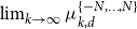 $\lim _{k \to \infty } \mu _{k,d}^{\{-N,\ldots , N\}}$
exists for all
$\lim _{k \to \infty } \mu _{k,d}^{\{-N,\ldots , N\}}$
exists for all $N \ge 0$
and is independent of
$N \ge 0$
and is independent of $N$
.
$N$
.
Note that $\mu _{k,d}^w$
is not affected by a scaling of
$\mu _{k,d}^w$
is not affected by a scaling of $w$
. Thus, we may assume that
$w$
. Thus, we may assume that $w$
is itself a probability distribution. Note in particular that this means it belongs to
$w$
is itself a probability distribution. Note in particular that this means it belongs to $\mathcal{E}$
(it is symmetric, and its support is an interval or all of
$\mathcal{E}$
(it is symmetric, and its support is an interval or all of $\mathbb{Z}$
). Our broad goal is to prove that the iterates of
$\mathbb{Z}$
). Our broad goal is to prove that the iterates of $\psi$
starting from
$\psi$
starting from $\varphi (w)$
converge pointwise. Along the way we also argue that all iterates stay in the set
$\varphi (w)$
converge pointwise. Along the way we also argue that all iterates stay in the set $\mathcal{S}_{0,1,c}$
, whose preimage under
$\mathcal{S}_{0,1,c}$
, whose preimage under $\varphi$
is a tight family of distributions. Consequently, we argue that
$\varphi$
is a tight family of distributions. Consequently, we argue that $f_k(\rho )$
converges in distribution and that
$f_k(\rho )$
converges in distribution and that $\mu ^0_{k,d}$
converges weakly.
$\mu ^0_{k,d}$
converges weakly.
The major step is to prove the following.
Proposition 2.7.
Fix $2 \le d \le 7$
. Let
$2 \le d \le 7$
. Let $w$
be a good sequence of weights normalized to be a probability distribution. There exists
$w$
be a good sequence of weights normalized to be a probability distribution. There exists $c \in (0,1)$
such that the
$c \in (0,1)$
such that the $\psi ^{(k)}({\mathsf R}(w))$
belongs to
$\psi ^{(k)}({\mathsf R}(w))$
belongs to $\mathcal{S}_{0,1,c}$
for all
$\mathcal{S}_{0,1,c}$
for all $k$
large enough and converges pointwise as
$k$
large enough and converges pointwise as $k \to \infty$
.
$k \to \infty$
.
Proof of Theorem
2.6
assuming Proposition
2.7. It is not hard to check that ${\mathsf R}^{-1}$
is continuous on its domain
${\mathsf R}^{-1}$
is continuous on its domain $\mathcal{R}$
(when both the domain and range are endowed with the pointwise topology). Since
$\mathcal{R}$
(when both the domain and range are endowed with the pointwise topology). Since $F^{(k)}(w) = {\mathsf R}^{-1} \circ \psi ^{(k)} \circ {\mathsf R}(w)$
, we conclude from Proposition2.7 that
$F^{(k)}(w) = {\mathsf R}^{-1} \circ \psi ^{(k)} \circ {\mathsf R}(w)$
, we conclude from Proposition2.7 that $F^{(k)}(w)$
converges pointwise and that
$F^{(k)}(w)$
converges pointwise and that $F^{(k)}(w)$
belongs to
$F^{(k)}(w)$
belongs to ${\mathsf R}^{-1}(\mathcal{S}_{0,1,c})$
for all
${\mathsf R}^{-1}(\mathcal{S}_{0,1,c})$
for all $k$
large enough. Observe that
$k$
large enough. Observe that ${\mathsf R}^{-1}(\mathcal{S}_{0,1,c})$
is a tight family of distributions. Thus, letting
${\mathsf R}^{-1}(\mathcal{S}_{0,1,c})$
is a tight family of distributions. Thus, letting $f_{k} \sim \mu _{k,d}^w$
and recalling Claim2.1 (or rather its straightforward extension from
$f_{k} \sim \mu _{k,d}^w$
and recalling Claim2.1 (or rather its straightforward extension from $\mu ^0_{k,d}$
to
$\mu ^0_{k,d}$
to $\mu ^w_{k,d}$
), this implies that
$\mu ^w_{k,d}$
), this implies that $f_k(\rho )$
converges in distribution as
$f_k(\rho )$
converges in distribution as $n \to \infty$
.
$n \to \infty$
.
It is now not too hard to see that $f_n$
converges locally. We very briefly give the idea. Fix
$f_n$
converges locally. We very briefly give the idea. Fix $r \ge 0$
and consider the restriction
$r \ge 0$
and consider the restriction $f_{k,r}$
of
$f_{k,r}$
of $f_k$
to
$f_k$
to $L_k$
, where
$L_k$
, where $L_r$
is the subtree of depth
$L_r$
is the subtree of depth $r$
(assume
$r$
(assume $k$
large). Then, for a given Lipschitz function
$k$
large). Then, for a given Lipschitz function $\xi$
on
$\xi$
on $L_r$
, we have that
$L_r$
, we have that $\mathbb{P}(f_{n,r}=\xi )$
is proportional
$\mathbb{P}(f_{n,r}=\xi )$
is proportional $\prod _v \mathbb{P}(f_{k-r}(\rho )=\xi (v))$
, where the product is over the leaves of
$\prod _v \mathbb{P}(f_{k-r}(\rho )=\xi (v))$
, where the product is over the leaves of $L_r$
. Since this product converges as
$L_r$
. Since this product converges as $k\to \infty$
, we see that the distribution of
$k\to \infty$
, we see that the distribution of $f_{k,r}$
converges as
$f_{k,r}$
converges as $n\to \infty$
, which shows that
$n\to \infty$
, which shows that $f_k$
converges locally.
$f_k$
converges locally.
To prove Proposition2.7 we employ the following strategy. First, we shall show that
 \begin{equation} \text{if $w$ is good then there exist $k \ge 0$ and $c \in [0,1)$ such that $\psi ^{(k)}({\mathsf R}(w)) \in \mathcal{S}_{0,1,c}$.} \end{equation}
This reduces the problem to understanding the iterations of $\psi$
starting from an initial point in
$\psi$
starting from an initial point in $\mathcal{S}_{0,1,c}$
. For this we will show that there exist numbers
$\mathcal{S}_{0,1,c}$
. For this we will show that there exist numbers $a_*,b_*,c_*$
with
$a_*,b_*,c_*$
with $0 \le a_*,c_* \le b_* \le 1$
such that
$0 \le a_*,c_* \le b_* \le 1$
such that
 \begin{equation} \text{for every $0 \le c \lt 1$ there exists $k$ such that $\psi ^{(k)}(\mathcal{S}_{0,1,c}) \subseteq \mathcal{S}_{a_*,b_*,c_*}$}, \end{equation}
and
 \begin{equation} \text{$\psi $ preserves the convex set $\mathcal{S}_{a_*,b_*,c_*}$ and is a contraction on it}. \end{equation}
The contraction referred to in (2.12) is with respect to the metric induced by the norm given by
 \begin{equation} \|x\| \,:\!=\, \begin{cases} \sup _{i \ge 1} |x_i| &\text{if }d=2 \\ |x_1| + \sup _{i \ge 2} |x_i| &\text{if }3 \le d \le 7 \end{cases}. \end{equation}
Let us remark that the two norms are equivalent (of course, in the case of $d=2$
, this is just the usual
$d=2$
, this is just the usual $\ell ^\infty$
-norm). However, the map
$\ell ^\infty$
-norm). However, the map $\psi$
is not a contraction with respect to the
$\psi$
is not a contraction with respect to the $\ell ^\infty$
norm when
$\ell ^\infty$
norm when $d \ge 4$
even very near the fixed point (see Table 4), and for this reason, we use a slightly modified norm (we use this norm also for
$d \ge 4$
even very near the fixed point (see Table 4), and for this reason, we use a slightly modified norm (we use this norm also for $d=3$
). Let us mention that the
$d=3$
). Let us mention that the $\ell ^1$
-norm is also a natural candidate, but that this would not allow to obtain the full stated result as
$\ell ^1$
-norm is also a natural candidate, but that this would not allow to obtain the full stated result as $\mathcal{S}_{0,1,c}$
is not in
$\mathcal{S}_{0,1,c}$
is not in $\ell ^1$
.
$\ell ^1$
.
Let us show how the above easily yields Proposition2.7.
Proof of Proposition
2.7
assuming(2.10)–(2.12). Let $w$
be a good sequence of weights normalized to be a probability distribution. Denote
$w$
be a good sequence of weights normalized to be a probability distribution. Denote $x^{(k)} \,:\!=\, \psi ^{(k)}(R(w))$
. By (2.10), there exists
$x^{(k)} \,:\!=\, \psi ^{(k)}(R(w))$
. By (2.10), there exists $k_0$
and
$k_0$
and $c$
such that
$c$
such that $x^{(k_0)} \in \mathcal{S}_{0,1,c}$
. By (2.11), there exists
$x^{(k_0)} \in \mathcal{S}_{0,1,c}$
. By (2.11), there exists $k_1$
such that
$k_1$
such that $x^{(k_0+k_1)} \in \mathcal{S}_{a_*,b_*,c_*}$
. By (2.12), there exists
$x^{(k_0+k_1)} \in \mathcal{S}_{a_*,b_*,c_*}$
. By (2.12), there exists $\lambda \in (0,1)$
such that
$\lambda \in (0,1)$
such that $x^{(k)} \in \mathcal{S}_{a_*,b_*,c_*}$
and
$x^{(k)} \in \mathcal{S}_{a_*,b_*,c_*}$
and $\|x^{(k+1)}-x^{(k)}\| \le \lambda \|x^{(k)}-x^{(k-1)}\|$
for all
$\|x^{(k+1)}-x^{(k)}\| \le \lambda \|x^{(k)}-x^{(k-1)}\|$
for all $k \ge k_0+k_1$
. Since
$k \ge k_0+k_1$
. Since $\mathcal{S}_{a_*,b_*,c_*} \subset \mathcal{S}_{0,1,c_*}$
, we have that
$\mathcal{S}_{a_*,b_*,c_*} \subset \mathcal{S}_{0,1,c_*}$
, we have that $x^{(k)} \in \mathcal{S}_{0,1,c_*}$
for all
$x^{(k)} \in \mathcal{S}_{0,1,c_*}$
for all $k$
large enough, and since
$k$
large enough, and since $\|\cdot \|$
makes
$\|\cdot \|$
makes $\mathcal{S}_{0,1,c_*}$
a complete metric space, we have that
$\mathcal{S}_{0,1,c_*}$
a complete metric space, we have that $x^{(k)}$
converges in this space, which clearly implies pointwise convergence.
$x^{(k)}$
converges in this space, which clearly implies pointwise convergence.
The next two sections are devoted to the proofs of (2.10)–(2.12). In Section 2.4, we prove (2.10) and (2.11), and in Section 2.5, we prove (2.12).
2.4 Getting absorbed into the basin of attraction
Proof of (2.10). For $n \ge 1$
, let
$n \ge 1$
, let $\mathcal{A}_n$
be the set of
$\mathcal{A}_n$
be the set of $x \in \mathcal{R}$
such that
$x \in \mathcal{R}$
such that $x_i=1$
for
$x_i=1$
for $i \le n$
and
$i \le n$
and $\sup _{i\gt n} x_i \lt 1$
. Note that
$\sup _{i\gt n} x_i \lt 1$
. Note that $\mathcal{A}_0 \cup \mathcal{A}_1 = \bigcup _{c \in [0,1)} \mathcal{S}_{0,1,c}$
. Let
$\mathcal{A}_0 \cup \mathcal{A}_1 = \bigcup _{c \in [0,1)} \mathcal{S}_{0,1,c}$
. Let $w$
be a good sequence of weights normalized to be a probability distribution. Note that
$w$
be a good sequence of weights normalized to be a probability distribution. Note that $R(w) \in \bigcup _{n \ge 0} \mathcal{A}_n$
. Thus, it suffices to show that
$R(w) \in \bigcup _{n \ge 0} \mathcal{A}_n$
. Thus, it suffices to show that
 \begin{align*} \psi (\mathcal{A}_n) \subset \mathcal{A}_{n-1} \qquad \text{for all }n \ge 2 . \end{align*}
Fix $n \ge 2$
and
$n \ge 2$
and $x \in \mathcal{A}_n$
. Denote
$x \in \mathcal{A}_n$
. Denote $c \,:\!=\, \sup _{i\gt n} x_i \lt 1$
. It is clear from (2.2) and (2.3) that
$c \,:\!=\, \sup _{i\gt n} x_i \lt 1$
. It is clear from (2.2) and (2.3) that $\psi _i(x)=1$
for
$\psi _i(x)=1$
for $i\le n-1$
and that
$i\le n-1$
and that $\psi _i(x)\lt 1$
for
$\psi _i(x)\lt 1$
for $i \ge n$
. Moreover, in the same manner as in the proof of Lemma2.2, one obtains a uniform upper bound on
$i \ge n$
. Moreover, in the same manner as in the proof of Lemma2.2, one obtains a uniform upper bound on $\psi _i(x)\lt 1$
for
$\psi _i(x)\lt 1$
for $i \ge n$
, namely,
$i \ge n$
, namely,
 \begin{align*} \psi _i(x) \le \left (\frac {1+c+c^2}{2+c}\right )^d . \end{align*}
This shows that $\psi (x) \in \mathcal{A}_{n-1}$
.
$\psi (x) \in \mathcal{A}_{n-1}$
.
We now move on to the proof of (2.11). Given Lemma2.2, the proof of (2.11) boils down to understanding the behaviour of the iterations of $\varphi$
applied to
$\varphi$
applied to $\mathcal{S}_{0,1,c}$
. It is not too hard to show that the iterations of
$\mathcal{S}_{0,1,c}$
. It is not too hard to show that the iterations of $\varphi$
do converge to a fixed point
$\varphi$
do converge to a fixed point $(a_*,b_*,c_*)$
if we start from
$(a_*,b_*,c_*)$
if we start from $a=0,b=1,c\gt 1/2$
(this part is true for all values of
$a=0,b=1,c\gt 1/2$
(this part is true for all values of $d$
). Nevertheless to have estimates of the derivative of
$d$
). Nevertheless to have estimates of the derivative of $\psi$
, we need good estimates on
$\psi$
, we need good estimates on $(a_*,b_*,c_*)$
. Iterations in a computer yield the estimates of
$(a_*,b_*,c_*)$
. Iterations in a computer yield the estimates of $(a_*,b_*,c_*)$
laid out in Table 1.
$(a_*,b_*,c_*)$
laid out in Table 1.
The fixed point of $\varphi$
. Simulated in computer by running ten thousand iterations started from
$\varphi$
. Simulated in computer by running ten thousand iterations started from $a=0,b=1,c=.9$

Table 1 Long description
A table with four columns and seven rows, including headers. The columns are labeled d, a subscript *, b subscript *, and c subscript *. The table presents the fixed points for different values of d. Row 1: d, 2; a subscript *, .5192; b subscript *, .6335; c subscript *, .988. Row 2: d, 3; a subscript *, .4374; b subscript *, .4649; c subscript *, .0344. Row 3: d, 4; a subscript *, .3762; b subscript *, .3828; c subscript *, .0060. Row 4: d, 5; a subscript *, .3294; b subscript *, .3310; c subscript *, 9.5 times 10 to the power of -4. Row 5: d, 6; a subscript *, .2932; b subscript *, .2935; c subscript *, 1.4 times 10 to the power of -4. Row 6: d, 7; a subscript *, .2645; b subscript *, .2646; c subscript *, 1.8 times 10 to the power of -5. Row 7: d, 8; a subscript *, .1027; b subscript *, .4906; c subscript *, 1.4 times 10 to the power of -4.
For $d \ge 8$
, iterations show that
$d \ge 8$
, iterations show that $a_*$
and
$a_*$
and $b_*$
are far apart, which is a manifestation of the non-convergence (in reality, as we have seen in Section 2.2, the actual value of
$b_*$
are far apart, which is a manifestation of the non-convergence (in reality, as we have seen in Section 2.2, the actual value of $x_1$
alternates between being close to
$x_1$
alternates between being close to $a_*$
and
$a_*$
and $b_*$
).
$b_*$
).
To make the result completely rigorous, we obtain rigorous estimates of $a_*,b_*,c_*$
, outlined in Table 2. While we could have obtained much better estimates (closer to the actual fixed point), it will turn out that these estimates are enough to bound the operator norm of the derivative of
$a_*,b_*,c_*$
, outlined in Table 2. While we could have obtained much better estimates (closer to the actual fixed point), it will turn out that these estimates are enough to bound the operator norm of the derivative of $\psi$
(with respect to the norm (2.13) on the base space). For larger values of
$\psi$
(with respect to the norm (2.13) on the base space). For larger values of $d$
(especially
$d$
(especially $d=7$
), we need slightly better precision.
$d=7$
), we need slightly better precision.
Proposition 2.8.
Fix $2 \le d\le 7$
. Let
$2 \le d\le 7$
. Let $(\hat a_*,\hat b_*,\hat c_*)$
be as in Table
2
. Then, for any
$(\hat a_*,\hat b_*,\hat c_*)$
be as in Table
2
. Then, for any $0 \le c\lt 1$
,
$0 \le c\lt 1$
, $\psi ^{(k)}(\mathcal{S}_{0,1,c}) \subset \mathcal{S}_{\hat a_*,\hat b_*,\hat c_*}$
for all large enough
$\psi ^{(k)}(\mathcal{S}_{0,1,c}) \subset \mathcal{S}_{\hat a_*,\hat b_*,\hat c_*}$
for all large enough $k$
.
$k$
.
The proof of Proposition2.8 is rather technical, so we postpone it to Section 6 on order not to disrupt the flow of the argument. Readers who are content with the computer estimates in Table 1 can skip Section 6 altogether. For estimates of the fixed point and some derivatives evaluated at the fixed point, please see Table 3.
Rigorous estimates of $a_*,b_*,c_*$
. Proofs can be found in Section 6
$a_*,b_*,c_*$
. Proofs can be found in Section 6
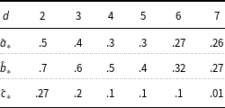
Table 2 Long description
A table with four rows and five columns. The columns are labeled d, a star, b star, and c star. The rows are labeled with values of d ranging from 2 to 7. The table presents estimates of a star, b star, and c star for each value of d. Row 1: d, 2; a star, 5; b star, 0.7; c star, 0.27. Row 2: d, 3; a star, 4; b star, 0.6; c star, 2. Row 3: d, 4; a star, 3; b star, 0.5; c star, 1. Row 4: d, 5; a star, 3; b star, 0.4; c star, 1. Row 5: d, 6; a star, 0.27; b star, 0.32; c star, 1. Row 6: d, 7; a star, 0.26; b star, 0.27; c star, 0.01.
The fixed point $x_*$
and some partial derivatives of
$x_*$
and some partial derivatives of $\psi$
at this point. Simulated in computer by running a million iterations
$\psi$
at this point. Simulated in computer by running a million iterations

Table 3 Long description
The table presents values of x1, x2, x3, x4, and their differences and ratios for different d values. It has 8 rows and 6 columns. The columns are labeled with d values ranging from 2 to 7. The rows are labeled with x1, x2, x3, x4, the difference of x1 and x2, the ratio of x2 to x1, and the ratio of x3 to x2. Row 1: d, 2, 3, 4, 5, 6, 7. Row 2: x1, .5992, .4555, .3803, .3303, .2936, .2646. Row 3: x2, .1712, .0327, .0059, 9.5 * 10^-4, 1.4 * 10^-4, 1.8 * 10^-5. Row 4: x3, .0222, 3.2 * 10^-5, 1.2 * 10^-9, 1.6 * 10^-16, 6.4 * 10^-24, 5.1 * 10^-34. Row 5: x4, 4.7 * 10^-4, 3.2 * 10^-14, 1.8 * 10^-36, 2.5 * 10^-76, 6.8 * 10^-140, 9.1 * 10^-234. Row 6: -x2/x1, .2655, .4704, .6213, .7467, .8575, .9577. Row 7: |x3/x2|, .4220, .4234, .4184, .4100, .3992, .3874. Row 8: |x4/x3|, .3357, .1467, 1.8 * 10^-7, .0108, .0022, 3.7 * 10^-4. Row 9: |x4/x2|, .1773, .0647, 4.6 * 10^-9, .0036, 6.3 * 10^-4, 9.7 * 10^-7.
2.5 Contraction via the derivatives
Our goal in this section is to prove (2.12). We do this by bounding the derivatives of $\psi$
. Recall the norm
$\psi$
. Recall the norm $\|\cdot \|$
defined in (2.13). It is straightforward to check that the Frechét derivative of the map
$\|\cdot \|$
defined in (2.13). It is straightforward to check that the Frechét derivative of the map $\psi$
evaluated at
$\psi$
evaluated at $x$
is the linear operator on the vector space spanned by
$x$
is the linear operator on the vector space spanned by $\mathcal{R}$
given by
$\mathcal{R}$
given by
 \begin{equation*} (D\psi _x(y))_i = (D\psi _i)_x(y) = \sum _{j \ge 1} \frac {\partial \psi _i}{\partial x_j} \cdot y_j. \end{equation*}
Note that $\partial \psi _i / \partial \psi _j = 0$
unless
$\partial \psi _i / \partial \psi _j = 0$
unless $|i-j| \le 1$
. Recall that the operator norm of
$|i-j| \le 1$
. Recall that the operator norm of $D\psi _x$
is
$D\psi _x$
is $\|D\psi _x\| \,:\!=\, \sup _{y : \|y\|=1} \|D\psi _x y\|$
. Here the norm we use is as in Equation (2.13).
$\|D\psi _x\| \,:\!=\, \sup _{y : \|y\|=1} \|D\psi _x y\|$
. Here the norm we use is as in Equation (2.13).
Proposition 2.9. $\|D\psi _x\| \lt .99$
for all
$\|D\psi _x\| \lt .99$
for all $x \in \mathcal{S}_{a,b,c}$
with
$x \in \mathcal{S}_{a,b,c}$
with $(a,b,c)$
as in Table
2
.
$(a,b,c)$
as in Table
2
.
From here it is simple to deduce (2.12).
Proof of
(2.12)assuming Proposition
2.9. Let $(a,b,c)$
be as in Table 2. The fact that
$(a,b,c)$
be as in Table 2. The fact that $\psi$
preserves
$\psi$
preserves $\mathcal{S}_{a,b,c}$
is the content of Proposition2.8. Let
$\mathcal{S}_{a,b,c}$
is the content of Proposition2.8. Let $x,y\in \mathcal{S}_{a,b,c}$
, and let
$x,y\in \mathcal{S}_{a,b,c}$
, and let $T$
denote a bounded linear functional on the vector space spanned by
$T$
denote a bounded linear functional on the vector space spanned by $\mathcal{R}$
, such that
$\mathcal{R}$
, such that $\|T\|=1$
(the operator norm is defined with respect to the norm given in (2.13)). Since
$\|T\|=1$
(the operator norm is defined with respect to the norm given in (2.13)). Since $\psi$
is differentiable, via the chain rule we have that
$\psi$
is differentiable, via the chain rule we have that
 \begin{align*} D(T\circ \psi )=T\circ D\psi . \end{align*}
For $t \in [0,1]$
, define
$t \in [0,1]$
, define
 \begin{align*} x(t)\,:\!=\,ty+(1-t)x\qquad \text{and}\qquad r(t)\,:\!=\,T\circ \psi (x(t)). \end{align*}
By the fundamental theorem of calculus,
 \begin{align*} T\circ \psi (y)- T\circ \psi (x) &=\int _{0}^{1}r'(t)dt \\ &=\int _{0}^{1} T\circ D\psi _{x(t)}\left (y-x\right )dt. \end{align*}
Thus, using that $\|T\|=1$
,
$\|T\|=1$
,
 \begin{align*} |T\circ \psi (y)-T\circ \psi (x)|&\leq \int _{0}^{1}\|T\circ D\psi _{x(t)}\| \cdot \|y-x\|dt \\ &\leq \sup _{t\in [0,1]} \|D\psi _{x(t)}\| \cdot \|y-x\|. \end{align*}
Since $\mathcal{S}_{a,b,c}$
is convex,
$\mathcal{S}_{a,b,c}$
is convex, $x(t)\in \mathcal{S}_{a,b,c}$
for all
$x(t)\in \mathcal{S}_{a,b,c}$
for all $t\in [0,1]$
, so we may replace the upper bound of the norm of the derivative on the path
$t\in [0,1]$
, so we may replace the upper bound of the norm of the derivative on the path $x(t)$
with the upper bound of the same on
$x(t)$
with the upper bound of the same on $\mathcal{S}_{a,b,c}$
. Finally, taking the supremum over all
$\mathcal{S}_{a,b,c}$
. Finally, taking the supremum over all $T$
such that
$T$
such that $\|T\|=1$
, we may conclude that
$\|T\|=1$
, we may conclude that
 \begin{equation*} \|\psi (x) - \psi (y)\| \le \sup _{y \in \mathcal{S}_{a,b,c}}\|D\psi _y\| \cdot \|x-y\|, \end{equation*}
which combined with Proposition2.9 gives that $\psi$
is a contraction on
$\psi$
is a contraction on $\mathcal{S}_{a,b,c}$
.
$\mathcal{S}_{a,b,c}$
.
The rest of this section is devoted to the proof of Proposition2.9. We begin by giving an upper bound for the operator norm of $D\psi _x$
in terms of the partial derivatives of
$D\psi _x$
in terms of the partial derivatives of $\psi$
.
$\psi$
.
Lemma 2.10.
For $d=2$
, the operator norm of
$d=2$
, the operator norm of $D\psi _x$
is
$D\psi _x$
is
 \begin{align*} \|D\psi _x\| &= \sup _{i \ge 1} \sum _{j \ge 1} \left |\frac {\partial \psi _i}{\partial x_j}\right | \\ &= \max \left \{ \left |\frac {\partial \psi _1}{\partial x_1}\right | + \left |\frac {\partial \psi _1}{\partial x_2}\right | ,\, \sup _{i \ge 2} \left (\left |\frac {\partial \psi _i}{\partial x_{i-1}}\right |+\left |\frac {\partial \psi _i}{\partial x_i}\right |+\left |\frac {\partial \psi _i}{\partial x_{i+1}}\right |\right ) \right \}\!. \end{align*}
For $d \ge 3$
, the operator norm of
$d \ge 3$
, the operator norm of $D\psi _x$
is
$D\psi _x$
is
 \begin{align*} \|D\psi _x\| &\le \max \left \{ \left |\frac {\partial \psi _1}{\partial x_1}\right | + \sup _{i \ge 2} \left |\frac {\partial \psi _i}{\partial x_1}\right | ,\, \sum _{j \ge 2} \left |\frac {\partial \psi _1}{\partial x_j}\right | + \sup _{i \ge 2} \sum _{j \ge 2} \left |\frac {\partial \psi _i}{\partial x_j}\right | \right \} \\ &= \max \left \{ \left |\frac {\partial \psi _1}{\partial x_1}\right | + \left |\frac {\partial \psi _2}{\partial x_1}\right | ,\, \left |\frac {\partial \psi _1}{\partial x_2}\right | + \sup _{i \ge 2} \sum _{j=i-1}^{i+1} \left |\frac {\partial \psi _i}{\partial x_j}\right | \mathbf{1}_{j \ge 2} \right \}\!. \end{align*}
Proof.
We only prove the case of $d \ge 3$
(the case
$d \ge 3$
(the case $d=2$
is similar and more standard as the norm is simply the
$d=2$
is similar and more standard as the norm is simply the $\ell ^\infty$
-norm). Denote
$\ell ^\infty$
-norm). Denote $T \,:\!=\, D\psi _x$
and
$T \,:\!=\, D\psi _x$
and $t_{i,j} \,:\!=\, \frac {\partial \psi _i}{\partial x_j}$
, so that
$t_{i,j} \,:\!=\, \frac {\partial \psi _i}{\partial x_j}$
, so that $(Ty)_i = \sum _j t_{i,j} y_j$
. Denote
$(Ty)_i = \sum _j t_{i,j} y_j$
. Denote $m_i \,:\!=\, \sum _{j \ge 2} |t_{i,j}|$
. Let
$m_i \,:\!=\, \sum _{j \ge 2} |t_{i,j}|$
. Let $y$
have norm 1. Write
$y$
have norm 1. Write $a\,:\!=\,|y_1|$
and
$a\,:\!=\,|y_1|$
and $b\,:\!=\,1-|a|$
, and note that
$b\,:\!=\,1-|a|$
, and note that $|y_i| \le b$
for all
$|y_i| \le b$
for all $i \ge 2$
. Then
$i \ge 2$
. Then
 \begin{align*} |(Ty)_i| = \bigg |\sum _j t_{i,j} y_j\bigg | \le |t_{i,1}y_1| + \sum _{j \ge 2} |t_{i,j} y_j| \le a|t_{i,1}| + b m_i . \end{align*}
Hence,
 \begin{align*} \|Ty\| = |(Ty)_1| + \sup _{i \ge 2} |(Ty)_i| &\le a|t_{1,1}| + b m_1 + \sup _{i \ge 2} (a|t_{i,1}| + b m_i) \\ &\le \max \bigg \{ |t_{1,1}|+\sup _{i \ge 2} |t_{i,1}|,\, m_1 + \sup _{i \ge 2} m_i \bigg \} , \end{align*}
as desired.
We now record the expressions for the derivatives.
 \begin{align} -\frac {\partial \psi _1}{\partial x_1} &= \frac {d(1-x_2)(1+x_1+x_1x_2)^{d-1}}{(1+2x_1)^{d+1}}, \end{align}
 \begin{align} \frac {\partial \psi _1}{\partial x_2} & = \frac {dx_1(1+x_1+x_1x_2)^{d-1}}{(1+2x_1)^d} , \end{align}
and for $n \ge 2$
,
$n \ge 2$
,
 \begin{align} \frac {\partial \psi _n}{\partial x_{n-1}} &= \frac {dx_{n-1}^{d-1}(1+x_n+x_nx_{n+1})^d}{(1+x_{n-1}+x_{n-1}x_n)^{d+1}} , \end{align}
 \begin{align} \frac {\partial \psi _n}{\partial x_n} &= \frac {dx_{n-1}^{d}(1+x_n+x_nx_{n+1})^{d-1}(1+x_{n-1}x_{n+1}+x_{n+1})}{(1+x_{n-1}+x_{n-1}x_n)^{d+1}}, \end{align}
 \begin{align} \frac {\partial \psi _n}{\partial x_{n+1}} &= \frac {dx_{n-1}^d x_n(1+x_n+x_nx_{n+1})^{d-1}}{(1+x_{n-1}+x_{n-1}x_n)^d}. \end{align}
The next two lemmas provide bounds on the partial derivatives of $\psi$
. While we assume throughout that
$\psi$
. While we assume throughout that $(a,b,c)$
is chosen according to Table 2, we use only minor information about the actual values, and keep bounds general where possible. We shall only plug in the exact values of these parameters at the very end. The simple properties we need are that
$(a,b,c)$
is chosen according to Table 2, we use only minor information about the actual values, and keep bounds general where possible. We shall only plug in the exact values of these parameters at the very end. The simple properties we need are that $c \lt 1/2$
and that
$c \lt 1/2$
and that
 \begin{equation} (d-2)a \le 1\quad \text{for }2 \le d \le 5,\qquad (d-2)a \ge 1+dac\quad \text{for }d=6,7. \end{equation}
 \begin{equation} b((1-c)d-2) \le 1\quad \text{for }d=2,3,4 . \end{equation}
 \begin{equation} 1+2b(1+c) \le d\quad \text{for }d \ge 3 . \end{equation}
Lemma 2.11.
Let $x \in \mathcal{S}_{a,b,c}$
with
$x \in \mathcal{S}_{a,b,c}$
with $(a,b,c)$
as in Table
2
. Then
$(a,b,c)$
as in Table
2
. Then
 \begin{align} \left |\frac {\partial \psi _1}{\partial x_1}\right | &\le \frac {d(1+a)^{d-1}}{(1+2a)^{d+1}} &&\text{for $2 \le d \le 5$.} \end{align}
 \begin{align} \left |\frac {\partial \psi _1}{\partial x_1}\right | & \le \frac {d(1-c)(1+a+ac)^{d-1}}{(1+2a)^{d+1}} &&\text{for $d = 6,7$.} \end{align}
 \begin{align} \left |\frac {\partial \psi _1}{\partial x_2}\right | & \le \frac {db(1+b+bc)^{d-1}}{(1+2b)^d} &&\text{for $2 \le d \le 4$}. \end{align}
 \begin{align} \left |\frac {\partial \psi _1}{\partial x_2}\right | & \le \frac {(d-1)^{d-1}}{d^{d-1}(1-c)} &&\text{for $5 \le d \le 7$.} \end{align}
Proof.
Recall the expression for $|\partial \psi _1/\partial x_1|$
from (2.14). Since this expression is decreasing in
$|\partial \psi _1/\partial x_1|$
from (2.14). Since this expression is decreasing in $x_1$
(using (2.7)) we have
$x_1$
(using (2.7)) we have
 \begin{equation} \left |\frac {\partial \psi _1}{\partial x_1}\right | \le \frac {d(1-x_2)(1+a+ax_2)^{d-1}}{(1+2a)^{d+1}} \;=\!:\; h(x_2) . \end{equation}
The function $h(x)$
is maximized at
$h(x)$
is maximized at
 \begin{equation*}x_* \,:\!=\, \frac {(d-2)a-1}{da}.\end{equation*}
By (2.19), we have that $x_*\lt 0$
for
$x_*\lt 0$
for $2 \le d \le 5$
and
$2 \le d \le 5$
and $x_*\gt c$
for
$x_*\gt c$
for $d=6,7$
. Note that
$d=6,7$
. Note that $h$
is increasing on
$h$
is increasing on $(\!-\infty ,x_*]$
and decreasing on
$(\!-\infty ,x_*]$
and decreasing on $[x_*,\infty )$
. Overall,
$[x_*,\infty )$
. Overall, $h$
is decreasing on
$h$
is decreasing on $[0,c]$
for
$[0,c]$
for $2 \le d \le 5$
and increasing on
$2 \le d \le 5$
and increasing on $[0,c]$
for
$[0,c]$
for $d=6,7$
. Thus,
$d=6,7$
. Thus, $|\partial \psi _1/\partial x_1| \le h(0)$
for
$|\partial \psi _1/\partial x_1| \le h(0)$
for $2 \le d \le 5$
and
$2 \le d \le 5$
and $|\partial \psi _1/\partial x_1| \le h(c)$
for
$|\partial \psi _1/\partial x_1| \le h(c)$
for $d=6,7$
. This establishes the claimed bound on
$d=6,7$
. This establishes the claimed bound on $|\partial \psi _1/\partial x_1|$
.
$|\partial \psi _1/\partial x_1|$
.
Next, recall the expression for $|\partial \psi _1/\partial x_2|$
from (2.15). Since this expression is increasing in
$|\partial \psi _1/\partial x_2|$
from (2.15). Since this expression is increasing in $x_2$
,
$x_2$
,
 \begin{equation*} \left |\frac {\partial \psi _1}{\partial x_2}\right | \le \frac {dx_1(1+x_1+cx_1)^{d-1}}{(1+2x_1)^d} \;=\!:\; \tilde h(x_1) . \end{equation*}
Differentiating $\tilde h$
, we get
$\tilde h$
, we get
 \begin{equation*} \tilde h'(x) =\frac {d(1+x+cx)^{d-2}}{(1+2x)^{d+1}} [x(2-(1-c)d) +1]. \end{equation*}
If $d=2$
, then clearly
$d=2$
, then clearly $\tilde h'(x) \ge 0$
for
$\tilde h'(x) \ge 0$
for $x \ge 0$
, so that
$x \ge 0$
, so that $\tilde h(x_1) \le \tilde h(b)$
. For
$\tilde h(x_1) \le \tilde h(b)$
. For $d \ge 3$
, we have a critical point at
$d \ge 3$
, we have a critical point at
 \begin{equation*} \tilde x_* \,:\!=\, \frac 1{(1-c)d-2}. \end{equation*}
Note that $2-(1-c)d \lt 0$
since
$2-(1-c)d \lt 0$
since $c\lt 1/2$
. Thus,
$c\lt 1/2$
. Thus, $\tilde x_*$
is positive and is in fact a maximum of
$\tilde x_*$
is positive and is in fact a maximum of $\tilde h$
. Furthermore,
$\tilde h$
. Furthermore, $\tilde x_*\gt b$
for
$\tilde x_*\gt b$
for $d=3,4$
by (2.20). Thus,
$d=3,4$
by (2.20). Thus, $\tilde h(x_1) \le \tilde h(b)$
for
$\tilde h(x_1) \le \tilde h(b)$
for $d \le 4$
, and
$d \le 4$
, and $\tilde h(x_1) \le \tilde h(\tilde x_*)$
for
$\tilde h(x_1) \le \tilde h(\tilde x_*)$
for $d \ge 5$
. This establishes the claimed bound on
$d \ge 5$
. This establishes the claimed bound on $|\partial \psi _1/\partial x_2|$
.
$|\partial \psi _1/\partial x_2|$
.
Lemma 2.12.
Let $x \in \mathcal{S}_{a,b,c}$
with
$x \in \mathcal{S}_{a,b,c}$
with $(a,b,c)$
as in Table
2
. For
$(a,b,c)$
as in Table
2
. For $n \ge 2$
,
$n \ge 2$
,
 \begin{align} \left |\frac {\partial \psi _n}{\partial x_{n-1}}\right | &\le \frac {4d(d-1)^{d-1}(1+c+c^2)^d}{(d+1)^{d+1}(1+c)^{d-1}} &&\text{for $d=2$}, \end{align}
 \begin{align} \left |\frac {\partial \psi _n}{\partial x_{n-1}}\right | & \le \frac {db^{d-1}(1+c+c^2)^d}{(1+b)(1+b+bc)^{d}} &&\text{for $3 \le d \le 7$,} \end{align}
 \begin{align} \left |\frac {\partial \psi _n}{\partial x_n}\right | & \le \left |\frac {\partial \psi _n}{\partial x_{n-1}}\right | \cdot b(1+c+bc). \end{align}
 \begin{align} \left |\frac {\partial \psi _n}{\partial x_{n+1}}\right | &\le \frac {db^d c(1+c+c^2)^{d-1}}{(1+b+bc)^d}. \end{align}
We remark that it is easy to show that any $x \in \psi (\mathcal{S}_{a,b,c})$
satisfies
$x \in \psi (\mathcal{S}_{a,b,c})$
satisfies $x_n \le c^d$
for
$x_n \le c^d$
for $n \ge 3$
, and that one could use this extra information to improve the bounds given in the lemma. This did not seem, however, to simplify other parts of the proof, and so we did not find any reason to do this. Furthermore, the bounds we stated are uniform in
$n \ge 3$
, and that one could use this extra information to improve the bounds given in the lemma. This did not seem, however, to simplify other parts of the proof, and so we did not find any reason to do this. Furthermore, the bounds we stated are uniform in $n \ge 2$
and governed by the case
$n \ge 2$
and governed by the case $n=2$
; the bounds can be significantly improved as
$n=2$
; the bounds can be significantly improved as $n$
increases.
$n$
increases.
Proof.
Set $\beta \,:\!=\, 1+x_n$
, and for
$\beta \,:\!=\, 1+x_n$
, and for $x \ge 0$
, define
$x \ge 0$
, define
 \begin{equation*} h(x) \,:\!=\, \frac {x^{d-1}}{(1+\beta x)^{d+1}} , \end{equation*}
so that
 \begin{align*} \left |\frac {\partial \psi _n}{\partial x_{n-1}}\right | = h(x_{n-1}) \cdot d(1+x_n+x_nx_{n+1})^d . \end{align*}
Note that $h$
is maximized at
$h$
is maximized at $x_* \,:\!=\, \frac {d-1}{2\beta }$
, and that it is increasing on
$x_* \,:\!=\, \frac {d-1}{2\beta }$
, and that it is increasing on $[0,x_*]$
and decreasing on
$[0,x_*]$
and decreasing on $[x_*,\infty )$
. For
$[x_*,\infty )$
. For $d \ge 3$
, we have that
$d \ge 3$
, we have that $x_{n-1} \le b \le x_*$
by (2.21), and hence,
$x_{n-1} \le b \le x_*$
by (2.21), and hence, $h(x_{n-1}) \le h(b)$
and
$h(x_{n-1}) \le h(b)$
and
 \begin{align} \left |\frac {\partial \psi _n}{\partial x_{n-1}}\right | & \le \frac {db^{d-1}(1+x_n+x_nx_{n+1})^d}{(1+b+bx_n)^{d+1}} \end{align}
 \begin{align} & \le \frac {db^{d-1}(1+c+c^2)^d}{(1+b)(1+b+bc)^{d}}, \end{align}
where we used $1+b+bx_n \ge 1+b$
,
$1+b+bx_n \ge 1+b$
, $x_{n+1} \le c$
and (2.7). For
$x_{n+1} \le c$
and (2.7). For $d=2$
, we do not know whether
$d=2$
, we do not know whether $x_* \ge b$
, so instead we just use that
$x_* \ge b$
, so instead we just use that $h(x_{n-1}) \le h(x_*)$
and plug in the value of
$h(x_{n-1}) \le h(x_*)$
and plug in the value of $x_*$
to get that
$x_*$
to get that
 \begin{align} \left |\frac {\partial \psi _n}{\partial x_{n-1}}\right | & \le \frac {d\left (\frac {d-1}{2(1+x_n)}\right )^{d-1}(1+x_n+x_nx_{n+1})^d}{\left (1+\frac {d-1}{2}\right )^{d+1}} \end{align}
 \begin{align} & = \frac {4d(d-1)^{d-1} (1+x_n+x_nx_{n+1})^d}{(d+1)^{d+1} (1+x_n)^{d-1}}\nonumber \\[8pt] & \le \frac {4d(d-1)^{d-1} (1+c+c^2)^d}{(d+1)^{d+1} (1+c)^{d-1}}, \end{align}
where we used $x_{n+1} \le c$
and (2.7).
$x_{n+1} \le c$
and (2.7).
To upper bound $\partial \psi _n/\partial x_n$
, note that
$\partial \psi _n/\partial x_n$
, note that
 \begin{align*} \left |\frac {\partial \psi _n}{\partial x_n}\right | = \left |\frac {\partial \psi _n}{\partial x_{n-1}}\right | \cdot \frac {x_{n-1}(x_{n-1}x_{n+1} + x_{n+1}+1)}{x_nx_{n+1}+x_n+1} , \end{align*}
and then, for the second term on the right-hand side, lower bound the denominator by 1 and upper bound the numerator using $x_{n-1} \le b$
and
$x_{n-1} \le b$
and $x_{n+1} \le c$
. Finally,
$x_{n+1} \le c$
. Finally,
 \begin{align} \left |\frac {\partial \psi _n}{\partial x_{n+1}}\right | &= \frac {dx_{n-1}^d x_n(1+x_n+x_nx_{n+1})^{d-1}}{(1+x_{n-1}+x_{n-1}x_n)^d} \nonumber\\[-7pt]\end{align}
 \begin{align} & \le \frac {db^d x_n(1+x_n+x_nx_{n+1})^{d-1}}{(1+b+bx_n)^d} \nonumber\\[-7pt]\end{align}
 \begin{align} & \le \frac {db^d c(1+c+c^2)^{d-1}}{(1+b+bc)^d}, \end{align}
where in the first inequality we used that $|\partial \psi _n/\partial x_{n+1}|$
is increasing in
$|\partial \psi _n/\partial x_{n+1}|$
is increasing in $x_{n-1}$
and that
$x_{n-1}$
and that $x_{n-1} \le b$
, and in the second inequality we used
$x_{n-1} \le b$
, and in the second inequality we used $x_n,x_{n+1} \le c$
and (2.7).
$x_n,x_{n+1} \le c$
and (2.7).
Proof of Proposition
2.9. Using Lemmas2.11 and 2.12, we get upper bounds on the partial derivatives $|\partial \psi _i/\partial x_j|$
, which when combined with Lemma2.10 yields an upper bound on the operator norm
$|\partial \psi _i/\partial x_j|$
, which when combined with Lemma2.10 yields an upper bound on the operator norm $\|D\psi _x\|$
(see Table 4).
$\|D\psi _x\|$
(see Table 4).
Proof of Theorem 1.1. The proof of the non-convergence part is in Section 2.2. The convergence part follows from the more general Theorem2.6.
Upper bounds on the partial derivatives and operator norm when $x \in \mathcal{S}_{a,b,c}$
with
$x \in \mathcal{S}_{a,b,c}$
with $(a,b,c)$
as in Table 2. The bounds on the partial derivatives are obtained by plugging in the values of
$(a,b,c)$
as in Table 2. The bounds on the partial derivatives are obtained by plugging in the values of $a,b,c$
into the bounds given by Lemmas2.11 and 2.12 (
$a,b,c$
into the bounds given by Lemmas2.11 and 2.12 ( $n \ge 2$
in the table) and rounding up. The bounds on the operator norm are then obtained by plugging in the former bounds into the bounds from Lemma2.10
$n \ge 2$
in the table) and rounding up. The bounds on the operator norm are then obtained by plugging in the former bounds into the bounds from Lemma2.10

Table 4 Long description
The table presents values for partial derivatives and operator norms across dimensions 2 through 7. It includes rows for partial derivatives with respect to various variables and the operator norm. Each column corresponds to a specific dimension, with values provided for each dimension. The table is structured with column headers indicating the dimensions and row labels indicating the type of derivative or norm being measured. The values are precise and specific to each dimension, showing how these mathematical properties change with increasing dimension.
3. Long-range order for graphs with large expansion
In this section, we prove Theorem1.3. Recall that $G$
is an infinite bipartite connect graph with maximum degree
$G$
is an infinite bipartite connect graph with maximum degree $d$
and Cheeger constant
$d$
and Cheeger constant $h$
. We fix a finite subset
$h$
. We fix a finite subset $G'$
of
$G'$
of $G$
. Recall that
$G$
. Recall that $\nu ^{a,b}_{G',M}$
is the uniform measure on all
$\nu ^{a,b}_{G',M}$
is the uniform measure on all $M$
-Lipschitz functions on
$M$
-Lipschitz functions on $G' \cup \partial G'$
whose values on
$G' \cup \partial G'$
whose values on $\partial G'$
are constrained to be in
$\partial G'$
are constrained to be in $\{a,\ldots ,b\}$
for white vertices or in
$\{a,\ldots ,b\}$
for white vertices or in $\{b-M,\dots ,a+M\}$
for black vertices.
$\{b-M,\dots ,a+M\}$
for black vertices.
We now fix two integers $a,b$
with
$a,b$
with $0 \le b-a \le 2M$
. To facilitate the description of these Gibbs measures, we shall consider the following sets:
$0 \le b-a \le 2M$
. To facilitate the description of these Gibbs measures, we shall consider the following sets:
 \begin{align*} \mathcal{O}(f)&\,:\!=\, \{v \in G' \text{ is black}, f(v) \not \in \{ b-M, \ldots , a+M\}\},\\ \mathcal{E}(f)&\,:\!=\, \{v \in G' \text{ is white}, f(v) \not \in \{a,\ldots ,b\}\}. \end{align*}
and define $B(f)\,:\!=\, \mathcal{O}(f) \cup \mathcal{E}(f)$
. Let
$B(f)\,:\!=\, \mathcal{O}(f) \cup \mathcal{E}(f)$
. Let $A(f,v)$
denote the distance two connected component of
$A(f,v)$
denote the distance two connected component of $B(f)$
containing
$B(f)$
containing $v$
. To elaborate: connect two vertices if they are at distance at most two, and let
$v$
. To elaborate: connect two vertices if they are at distance at most two, and let $A(f,v)$
denote the connected component of
$A(f,v)$
denote the connected component of $v$
thus formed. Our goal in the next proposition will be to prove that the size of
$v$
thus formed. Our goal in the next proposition will be to prove that the size of $A(f,v)$
has exponential tail once
$A(f,v)$
has exponential tail once $h$
is large enough compared to
$h$
is large enough compared to $M$
.
$M$
.
Proposition 3.1.
Assume that $h+1 \ge 2(2M+1)\log (d^4(4M+1))$
, and let
$h+1 \ge 2(2M+1)\log (d^4(4M+1))$
, and let $f \sim \nu ^{a,b}_{G',M}$
. Then for all
$f \sim \nu ^{a,b}_{G',M}$
. Then for all $v_0 \in G'$
and
$v_0 \in G'$
and $N \ge 1$
,
$N \ge 1$
,
 \begin{equation*} \mathbb{P}(|A(f,v_0)| = N) \le \exp \left (-\frac {(h+1)N}{2(2M+1)}\right ). \end{equation*}
The upshot of Proposition3.1 is that most of the black vertices take values in $\{b-M,\ldots ,a+M\}$
and most of the white vertices take values in
$\{b-M,\ldots ,a+M\}$
and most of the white vertices take values in $\{a,\ldots ,b\}$
.
$\{a,\ldots ,b\}$
.
Let us illustrate some special cases. If $a=b=0$
and
$a=b=0$
and $M=1$
(1-Lipschitz case with 0 boundary conditions on even vertices), most of the white vertices take the value 0 and the black vertices take values in
$M=1$
(1-Lipschitz case with 0 boundary conditions on even vertices), most of the white vertices take the value 0 and the black vertices take values in $\{-1,0,1\}$
(roughly uniformly at random as they are likely to be surrounded by 0s). Also, if
$\{-1,0,1\}$
(roughly uniformly at random as they are likely to be surrounded by 0s). Also, if $a=0,b=1$
(as in Theorem1.2), then both white and black vertices are likely to take values in
$a=0,b=1$
(as in Theorem1.2), then both white and black vertices are likely to take values in $\{0,1\}$
. In general, if
$\{0,1\}$
. In general, if $b-a = M$
, the white and black vertices play a symmetric role in the measure (and in fact bipartiteness of
$b-a = M$
, the white and black vertices play a symmetric role in the measure (and in fact bipartiteness of $G$
is not needed).
$G$
is not needed).
Proof of Proposition
3.1. We begin with an elementary fact (see, e.g., [Reference Peled, Samotij and Yehudayoff23, Lemma 1.8]). Let $\mathcal{L}$
denote the set of
$\mathcal{L}$
denote the set of $M$
-Lipschitz functions on
$M$
-Lipschitz functions on $G'$
satisfying the required boundary constraints. Let
$G'$
satisfying the required boundary constraints. Let $\mathcal{E}$
be a subset of
$\mathcal{E}$
be a subset of $\mathcal{L}$
and suppose that
$\mathcal{L}$
and suppose that $T$
is a map from
$T$
is a map from $\mathcal{E}$
to subsets of
$\mathcal{E}$
to subsets of $\mathcal{L}$
. Also assume that there exist
$\mathcal{L}$
. Also assume that there exist $s,t\gt 0$
such that
$s,t\gt 0$
such that $|T(g)| \ge t$
for all
$|T(g)| \ge t$
for all $g \in \mathcal{E}$
, and
$g \in \mathcal{E}$
, and $|\{g \in \mathcal{A}\,:\, g' \in T(g) \}| \le s$
for all
$|\{g \in \mathcal{A}\,:\, g' \in T(g) \}| \le s$
for all $g' \in \mathcal{L}$
. Then
$g' \in \mathcal{L}$
. Then
 \begin{equation*} \mathbb{P}(f \in \mathcal{E}) = \frac {|\mathcal{E}|}{|\mathcal{L}|} \le \frac st.\end{equation*}
Throughout, we write $A(f)$
for
$A(f)$
for $A(f,v_0)$
and observe that
$A(f,v_0)$
and observe that $A(f)$
cannot contain any vertex of
$A(f)$
cannot contain any vertex of $\partial G'$
by definition. Fix a distance two connected set
$\partial G'$
by definition. Fix a distance two connected set $A$
containing
$A$
containing $v_0$
but not intersecting
$v_0$
but not intersecting $\partial G'$
, and let
$\partial G'$
, and let $\mathcal{E} \,:\!=\, \{g \in \mathcal{L}\,:\, A(g)=A\}$
. We shall construct a map
$\mathcal{E} \,:\!=\, \{g \in \mathcal{L}\,:\, A(g)=A\}$
. We shall construct a map $T$
as described in the previous paragraph so that
$T$
as described in the previous paragraph so that $s/t$
is small, where
$s/t$
is small, where $s,t$
are as in the previous paragraph. Consequently,
$s,t$
are as in the previous paragraph. Consequently,
 \begin{equation*}\mathbb{P}(A(f) =A) = \mathbb{P}(f \in \mathcal{E}) \le \frac st.\end{equation*}
Our goal is to make $\frac st$
exponentially small in the size of
$\frac st$
exponentially small in the size of $A$
with a suitably large constant, so that we can then apply a union bound over all possible realizations of
$A$
with a suitably large constant, so that we can then apply a union bound over all possible realizations of $A(f)$
and conclude.
$A(f)$
and conclude.
Let us describe the map $T$
. For
$T$
. For $g \in \mathcal{E}$
, let
$g \in \mathcal{E}$
, let $T(g)$
be the set of
$T(g)$
be the set of $g' \in \mathcal{L}$
satisfying
$g' \in \mathcal{L}$
satisfying
 \begin{equation} g'(x) \begin{cases} = g(x) &\text{if }x \not \in A \cup \partial A\\ \in \{a,\dots ,b\} &\text{if }x \in A \cup \partial A, x \text{ white,}\\ \in \{ b-M,\dots ,a+M\} &\text{if } x \in A \cup \partial A, x \text{ black.}\\ \end{cases} \end{equation}
The point of this definition is that, as we will see, it allows much more possibilities in $A \cup \partial A$
for
$A \cup \partial A$
for $g' \in T(g)$
compared to
$g' \in T(g)$
compared to $g$
. Specifically, we claim
$g$
. Specifically, we claim $T$
satisfies the requirement with
$T$
satisfies the requirement with
 \begin{equation} s \,:\!=\, (4M+1)^{|A|} (b-a)^{|\{v \in \partial A: v \text{ white}\}|}(a-b+2M)^{|\{v \in \partial A: v \text{ black}\}|}, \end{equation}
and
 \begin{equation} t \,:\!=\, (b-a+1)^{|\{v \in A \cup \partial A: v \text{ white}\}|}(a-b+2M+1)^{|\{v \in A \cup \partial A: v \text{ black}\}|}. \end{equation}
Before proving this claim, let us show how it yields the proposition. We have
 \begin{equation*} \frac {s}{t} \le (4M+1)^{|A|} \left (\frac {b-a}{b-a+1}\right )^{|\{v \in A\cup \partial A, v \text{ white}\}|}\left (\frac {a-b+2M}{a-b+2M+1}\right )^{|\{v \in A\cup \partial A, v \text{ black}\}|} \end{equation*}
Since $x \mapsto \frac {x}{x+1}$
is increasing and
$x \mapsto \frac {x}{x+1}$
is increasing and $0\le b-a \le 2M$
, and using the fact that
$0\le b-a \le 2M$
, and using the fact that $|\partial A| \ge h |A|$
(since recall that
$|\partial A| \ge h |A|$
(since recall that $A$
cannot contain any vertex in the boundary),
$A$
cannot contain any vertex in the boundary),
 \begin{equation} \mathbb{P}(A(f) = A) \le \frac {s}{t} \le (4M+1)^{|A|} \left (\frac {2M}{2M+1}\right )^{|A|+|\partial A|} \le e^{|A| \log (4M+1) - \frac {(h+1)|A|}{2M+1}} \end{equation}
Finally, the number of distance two connected sets $A$
with
$A$
with $|A|=N$
and
$|A|=N$
and $v_0 \in A$
is at most
$v_0 \in A$
is at most $d^{4N}$
. Union bounding, we get
$d^{4N}$
. Union bounding, we get
 \begin{equation*} \mathbb{P}(|A(f)| = N) \le e^{N(4 \log d + \log (4M+1) - \frac {h+1}{2M+1})} \le \exp \left (- \frac {(h+1)N}{2(2M+1)}\right )\!, \end{equation*}
as desired.
It remains to prove that $T$
satisfies the required upper and lower bounds with (3.2) and (3.3). We begin with the lower bound. Let
$T$
satisfies the required upper and lower bounds with (3.2) and (3.3). We begin with the lower bound. Let $g \in \mathcal{E}$
. Since
$g \in \mathcal{E}$
. Since $|x-y| \le M$
for
$|x-y| \le M$
for $x \in \{a,\dots ,b\}$
and
$x \in \{a,\dots ,b\}$
and $y \in \{b-M,\dots ,a+M\}$
, and since
$y \in \{b-M,\dots ,a+M\}$
, and since $g(v) \in \{a,\dots ,b\}$
for any white
$g(v) \in \{a,\dots ,b\}$
for any white $v \in \partial (A \cup \partial A)$
and
$v \in \partial (A \cup \partial A)$
and $g(v) \in \{b-M,\dots ,a+M\}$
for any black
$g(v) \in \{b-M,\dots ,a+M\}$
for any black $v \in \partial (A \cup \partial A)$
, we see that every function satisfying (3.1) must necessarily belong to
$v \in \partial (A \cup \partial A)$
, we see that every function satisfying (3.1) must necessarily belong to $\mathcal{L}$
. Hence,
$\mathcal{L}$
. Hence,
 \begin{equation*} |T(g)| = (b-a+1)^{|\{v \in A \cup \partial A: v \text{ white}\}|}(a-b+2M+1)^{|\{v \in A \cup \partial A: v \text{ black}\}|} = t. \end{equation*}
We now move on to the upper bound. Fix $g' \in \mathcal{L}$
. We need to upper bound the number of
$g' \in \mathcal{L}$
. We need to upper bound the number of $g \in \mathcal{E}$
such that
$g \in \mathcal{E}$
such that $g' \in T(g)$
. Clearly,
$g' \in T(g)$
. Clearly, $g$
is uniquely determined outside
$g$
is uniquely determined outside $A \cup \partial A$
. Note that if a vertex
$A \cup \partial A$
. Note that if a vertex $u$
in
$u$
in $A$
is at distance 2 from the complement of
$A$
is at distance 2 from the complement of $A \cup \partial A$
, then the number of possible values of
$A \cup \partial A$
, then the number of possible values of $g(u)$
is at most
$g(u)$
is at most $4M+1$
. By choosing the values of
$4M+1$
. By choosing the values of $g$
on
$g$
on $A$
one after another, in any order consistent with their distance from the complement of
$A$
one after another, in any order consistent with their distance from the complement of $A \cup \partial A$
, we see that there are at most
$A \cup \partial A$
, we see that there are at most $(4M+1)^{|A|}$
possible choices for
$(4M+1)^{|A|}$
possible choices for $g$
on
$g$
on $A$
. To show that
$A$
. To show that $|\{ g\in \mathcal{E} \,:\, g' \in T(g)\}| \le s$
, it remains to show that, given
$|\{ g\in \mathcal{E} \,:\, g' \in T(g)\}| \le s$
, it remains to show that, given $g$
outside
$g$
outside $\partial A$
, the number of choices for
$\partial A$
, the number of choices for $g$
on
$g$
on $\partial A$
is at most
$\partial A$
is at most $\prod _{v \in \partial A} \ell _v$
, where
$\prod _{v \in \partial A} \ell _v$
, where
 \begin{equation*} l_v\,:\!=\, \begin{cases} b-a &\text{if $v$ is white }\\ 2M+a-b &\text{if $v$ is black}. \end{cases} \end{equation*}
For this, it suffices to prove a vertex-by-vertex bound, namely, that the number of choices for $g(v)$
is at most
$g(v)$
is at most $\ell _v$
for any
$\ell _v$
for any $v \in \partial A$
. To this end, fix
$v \in \partial A$
. To this end, fix $v \in \partial A$
, and let
$v \in \partial A$
, and let $u \in A$
be any neighbour of
$u \in A$
be any neighbour of $v$
(which exists since
$v$
(which exists since $v \in \partial A$
). Suppose first that
$v \in \partial A$
). Suppose first that $v$
is white. First note that since
$v$
is white. First note that since $v \in \partial A$
and
$v \in \partial A$
and $v$
is white,
$v$
is white, $g(v) \in \{a,\ldots ,b\}$
. Similarly, since
$g(v) \in \{a,\ldots ,b\}$
. Similarly, since $u \in A$
and
$u \in A$
and $u$
is black,
$u$
is black, $g(u) \notin \{b-M,\dots ,a+M\}$
. Consequently,
$g(u) \notin \{b-M,\dots ,a+M\}$
. Consequently,
 \begin{align*} a+1 \le g(u) - M \le g(v) \le b, \qquad \text{if $g(u) \ge a+M+1$},\\ a \le g(v) \le g(u)+M \le b-1, \qquad \text{if $g(u) \le b-M-1$.} \end{align*}
(One consequence of the above inequalities is that $v$
cannot be white if
$v$
cannot be white if $a=b$
.) Therefore, the number of possible values of
$a=b$
.) Therefore, the number of possible values of $g(v)$
is at most
$g(v)$
is at most $\ell _v$
, as claimed. Suppose next that
$\ell _v$
, as claimed. Suppose next that $v$
is black. We similarly have that
$v$
is black. We similarly have that $g(v) \in \{b-M,\dots ,a+M\}$
and
$g(v) \in \{b-M,\dots ,a+M\}$
and $g(u) \notin \{a,\dots ,b\}$
, so that
$g(u) \notin \{a,\dots ,b\}$
, so that
 \begin{align*} b-M+1 \le g(u) - M \le g(v) \le a+M \qquad \text{if $g(u) \ge b+1$, }\\ b-M \le g(v) \le g(u)+M \le a+M-1 \qquad \text{if $g(u) \le a-1$.} \end{align*}
(Again, $v$
cannot be black if
$v$
cannot be black if $b-a=2M$
.) Therefore, the number of possible values of
$b-a=2M$
.) Therefore, the number of possible values of $g(v)$
is again at most
$g(v)$
is again at most $\ell _v$
, as claimed.
$\ell _v$
, as claimed.
The following corollary is a simple generalization of (3.4) and is what we will actually need in the proof of Theorem1.3.
Corollary 3.2.
Let $A_1 ,A_2,\ldots , A_k$
be distance two disjoint, distance two connected sets of total size
$A_1 ,A_2,\ldots , A_k$
be distance two disjoint, distance two connected sets of total size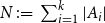 $N \,:\!=\, \sum _{i=1}^k|A_i|$
. Then the probability that
$N \,:\!=\, \sum _{i=1}^k|A_i|$
. Then the probability that $A_1,\ldots , A_k$
are distance two connected components of
$A_1,\ldots , A_k$
are distance two connected components of $B(f)$
is at most
$B(f)$
is at most
 \begin{equation*} \exp \left (N\left (\log\! (4M+1) - \dfrac {h+1}{2M+1}\right )\right ). \end{equation*}
Proof of Theorem
1.3. Let $(G_k)$
be an exhaustion. Note that it is enough to prove the following: for all
$(G_k)$
be an exhaustion. Note that it is enough to prove the following: for all $v \in V$
,
$v \in V$
, $R\gt 0$
and for all connected
$R\gt 0$
and for all connected $H,H'$
such that
$H,H'$
such that $B(v,R) \subset B(v,R') \subset H\subset H' \subset G$
,
$B(v,R) \subset B(v,R') \subset H\subset H' \subset G$
, $\nu _{H,M}^{a,b}$
can be coupled with
$\nu _{H,M}^{a,b}$
can be coupled with $\nu _{H',M}^{a,b}$
so that they agree on
$\nu _{H',M}^{a,b}$
so that they agree on $B(v, R)$
with probability tending to
$B(v, R)$
with probability tending to $1$
as
$1$
as $R' \to \infty$
.
$R' \to \infty$
.
To construct the coupling, let $f \sim \nu _{H, M}^{a,b}$
and
$f \sim \nu _{H, M}^{a,b}$
and $f' \sim \nu _{H',M}^{a,b}$
be sampled independently, and let
$f' \sim \nu _{H',M}^{a,b}$
be sampled independently, and let $B(f)$
and
$B(f)$
and $B(f')$
be the set of ‘atypical’ vertices as defined before Proposition3.1. Let
$B(f')$
be the set of ‘atypical’ vertices as defined before Proposition3.1. Let $U = B(v,R)$
, and let
$U = B(v,R)$
, and let $A(f,f',U)$
be the union of the distance two connected components of
$A(f,f',U)$
be the union of the distance two connected components of $B(f) \cup B(f')$
intersecting
$B(f) \cup B(f')$
intersecting $U$
. Then for any
$U$
. Then for any $A$
, using Corollary3.2 (and
$A$
, using Corollary3.2 (and $\frac {h+1}{2M+1} \ge \frac {h}{3M}$
),
$\frac {h+1}{2M+1} \ge \frac {h}{3M}$
),
 \begin{align*} \mathbb{P}(A(f,f',U) = A) &\le \sum _{A_1 \cup A_2 = A} \exp\! \left((|A_1| +|A_2|)\left(\log (4M+1) - \dfrac h{3M}\right)\right) \\ &\le 3^{|A|} \exp \!\left(|A|\left(\log (4M+1) - \dfrac {h}{3M}\right)\right)\! . \end{align*}
Here, $A_1$
and
$A_1$
and $A_2$
are
$A_2$
are $A(f,f',U) \cap B(f)$
and
$A(f,f',U) \cap B(f)$
and $A(f,f',U) \cap B(f')$
, respectively. Since there are at most
$A(f,f',U) \cap B(f')$
, respectively. Since there are at most $(2N)^{|U|}d^{4N}$
possible choices for such an
$(2N)^{|U|}d^{4N}$
possible choices for such an $A$
of a given size
$A$
of a given size $N$
(see Lemma3.3 below),
$N$
(see Lemma3.3 below),
 \begin{align*} \mathbb{P}(|A(f,f',U)| = N) &\le \exp\! \left (N \left(\log (3(4M+1)) - \dfrac h{3M} + 4\log d\right) + |U|\log (2N)\right ) \\&\le \exp\! \left(-\dfrac {hN}{6M} + |U|\log (2N)\right)\!. \end{align*}
Since $U$
is fixed, this bound decays exponentially in
$U$
is fixed, this bound decays exponentially in $N$
. In particular, as
$N$
. In particular, as $R' \to \infty$
,
$R' \to \infty$
,
 \begin{equation*} \mathbb{P}(A(f,f',U) \subset B(v,R')) \to 1. \end{equation*}
It remains to show that $f$
and
$f$
and $f'$
can be coupled so that they agree on
$f'$
can be coupled so that they agree on $B(v,R)$
on the event
$B(v,R)$
on the event $\{(A(f,f',U) \subset B(v,R')\}$
. We proceed via exploration from the boundary. Let
$\{(A(f,f',U) \subset B(v,R')\}$
. We proceed via exploration from the boundary. Let $X$
be the union of the distance two connected components of
$X$
be the union of the distance two connected components of $B(f) \cup B(f') \cup (G \setminus H)$
containing
$B(f) \cup B(f') \cup (G \setminus H)$
containing $G \setminus H$
. Note that, by definition of
$G \setminus H$
. Note that, by definition of $A(f,f',U)$
, we have that
$A(f,f',U)$
, we have that $X$
is disjoint from
$X$
is disjoint from $B(v,R+2)$
whenever
$B(v,R+2)$
whenever $A(f,f',U) \subset B(v,R'-2)$
. Denote
$A(f,f',U) \subset B(v,R'-2)$
. Denote $\tilde X \,:\!=\, X \cup \partial X$
,
$\tilde X \,:\!=\, X \cup \partial X$
, $\bar X \,:\!=\, \tilde X \cup \partial \tilde X$
and
$\bar X \,:\!=\, \tilde X \cup \partial \tilde X$
and $Y \,:\!=\, G \setminus \bar X$
. Note that
$Y \,:\!=\, G \setminus \bar X$
. Note that $X$
is measurable with respect to
$X$
is measurable with respect to $(B(f) \cup B(f')) \cap \bar X$
. Now condition on
$(B(f) \cup B(f')) \cap \bar X$
. Now condition on $X$
and on
$X$
and on $(f|_{\tilde X},f'|_{\tilde X})$
and suppose that
$(f|_{\tilde X},f'|_{\tilde X})$
and suppose that $X$
is disjoint from
$X$
is disjoint from $B(v,R+2)$
. We claim that
$B(v,R+2)$
. We claim that $f|_Y$
and
$f|_Y$
and $f'|_Y$
are conditionally distributed according to
$f'|_Y$
are conditionally distributed according to $\nu ^{a,b}_{Y,M}$
(in fact, they are also conditionally independent, but we do not need this), and in particular,
$\nu ^{a,b}_{Y,M}$
(in fact, they are also conditionally independent, but we do not need this), and in particular, $f|_Y$
and
$f|_Y$
and $f'|_Y$
can be coupled to agree on
$f'|_Y$
can be coupled to agree on $Y$
(which contains
$Y$
(which contains $B(v,R)$
). We prove this for
$B(v,R)$
). We prove this for $f|_Y$
(the proof for
$f|_Y$
(the proof for $f'_Y$
is identical). Indeed, every even
$f'_Y$
is identical). Indeed, every even $v \in \partial\! Y$
has
$v \in \partial\! Y$
has $f(v) \in \{a,\dots ,b\}$
, since
$f(v) \in \{a,\dots ,b\}$
, since $\partial Y \subset \partial \tilde X \subset (B(f) \cup B(f'))^c$
. On the other hand, any value in
$\partial Y \subset \partial \tilde X \subset (B(f) \cup B(f'))^c$
. On the other hand, any value in $\{a,\dots ,b\}$
is possible for
$\{a,\dots ,b\}$
is possible for $f(v)$
, since any
$f(v)$
, since any $u \in N(v) \setminus Y \subset \bar X \setminus X \subset (B(f) \cup B(f'))^c$
, is odd, and satisfies
$u \in N(v) \setminus Y \subset \bar X \setminus X \subset (B(f) \cup B(f'))^c$
, is odd, and satisfies $f(u) \in \{b-M,\dots ,a+M\}$
. Similarly, any odd vertex in
$f(u) \in \{b-M,\dots ,a+M\}$
. Similarly, any odd vertex in $\partial Y$
must take a values in
$\partial Y$
must take a values in $\{b-M, \ldots , a+M\}$
and is free to take any value there. Since there are no other constraints (beyond the obvious Lipschitz constraint), the conditional law of
$\{b-M, \ldots , a+M\}$
and is free to take any value there. Since there are no other constraints (beyond the obvious Lipschitz constraint), the conditional law of $f|_Y$
is
$f|_Y$
is $\nu ^{a,b}_{Y,M}$
. This completes the proof of convergence.
$\nu ^{a,b}_{Y,M}$
. This completes the proof of convergence.
Now we show part (b) of the theorem, which is an easy consequence of Proposition3.1. Let $f \sim \nu ^{a,b}_{G,M}$
. Fix an odd vertex
$f \sim \nu ^{a,b}_{G,M}$
. Fix an odd vertex $u$
and denote
$u$
and denote $\mathcal{N} \,:\!=\, \{\, f(v) \,:\, v \in N(u) \}$
. Let
$\mathcal{N} \,:\!=\, \{\, f(v) \,:\, v \in N(u) \}$
. Let $\mathcal{N}^-$
and
$\mathcal{N}^-$
and $\mathcal{N}^+$
be the minimum and maximum elements in
$\mathcal{N}^+$
be the minimum and maximum elements in $\mathcal{N}$
, respectively. Since
$\mathcal{N}$
, respectively. Since $f(u)$
is conditionally uniformly distributed in
$f(u)$
is conditionally uniformly distributed in $\{\mathcal{N}^+-M,\dots ,\mathcal{N}^-+M\}$
given
$\{\mathcal{N}^+-M,\dots ,\mathcal{N}^-+M\}$
given $\mathcal{N}$
, we see that
$\mathcal{N}$
, we see that
 \begin{align*} \mathbb{P}(\{\mathcal{N}^-,\dots ,\mathcal{N}^+\} \subsetneq \{a,\dots ,b\}) &\le (2M+1) \cdot \mathbb{P}(f(u) \notin \{b-M,\dots ,a+M\}) \\ &\le (2M+1) \cdot \mathbb{P}(|A(f,u)|\ge 1)) \\&\le \frac {2M+1}{e^{h/6M}-1} . \end{align*}
On the other hand,
 \begin{align*} \mathbb{P}(\{\mathcal{N}^-,\dots ,\mathcal{N}^+\} \not \subset \{a,\dots ,b\}) &= \mathbb{P}(\mathcal{N}^- \lt a\text{ or }\mathcal{N}^+\gt b) \\ &= \mathbb{P}(f(v) \notin \{a,\dots ,b\}\text{ for some }v \in N(u)) \\ &\le \sum _{v \in N(u)} \mathbb{P}(|A(f,v)|\ge 1)) \\&\le \frac {d}{e^{h/6M}-1} . \end{align*}
Together, we get that
 \begin{align*} \mathbb{P}(\{\mathcal{N}^-,\dots ,\mathcal{N}^+\} \neq \{a,\dots ,b\}) \le \frac {d+2M+1}{e^{h/6M}-1} \le \frac {d+2M+1}{3d^4(4M+1)-1} \lt \frac 12 , \end{align*}
which means that $\{a,\dots ,b\}$
is the largest atom of
$\{a,\dots ,b\}$
is the largest atom of $\{\mathcal{N}^-,\dots ,\mathcal{N}^+\}$
, so that it is uniquely determined by
$\{\mathcal{N}^-,\dots ,\mathcal{N}^+\}$
, so that it is uniquely determined by $\nu ^{a,b}_{G,M}$
.
$\nu ^{a,b}_{G,M}$
.
Lemma 3.3.
Let $\mathcal{G}$
be a graph of maximum degree at most
$\mathcal{G}$
be a graph of maximum degree at most $\Delta$
. Let
$\Delta$
. Let $U \subset V(\mathcal{G})$
. The number of sets
$U \subset V(\mathcal{G})$
. The number of sets $A \subset V(\mathcal{G})$
of a given size
$A \subset V(\mathcal{G})$
of a given size $N$
such that each connected component of
$N$
such that each connected component of $A$
intersects
$A$
intersects $U$
is at most
$U$
is at most $(2N)^{|U|} \Delta ^{2N}$
.
$(2N)^{|U|} \Delta ^{2N}$
.
Proof.
Let $U=\{u_1,\dots ,u_m\}$
be some enumeration of
$U=\{u_1,\dots ,u_m\}$
be some enumeration of $U$
. Given a set
$U$
. Given a set $B\subset V(\mathcal{G})$
that intersects
$B\subset V(\mathcal{G})$
that intersects $U$
, denote
$U$
, denote $I(B)\,:\!=\,\min \{1 \le i \le m : u_i \in B \}$
. Given a set
$I(B)\,:\!=\,\min \{1 \le i \le m : u_i \in B \}$
. Given a set $A$
as in the lemma, define
$A$
as in the lemma, define $(N_1,\dots ,N_m)$
by letting
$(N_1,\dots ,N_m)$
by letting $N_i=|C|$
if there exists a connected component
$N_i=|C|$
if there exists a connected component $C$
of
$C$
of $A$
such that
$A$
such that $I(C)=i$
, and
$I(C)=i$
, and $N_i=0$
otherwise. Note that
$N_i=0$
otherwise. Note that $N_1+\dots +N_m=N$
. The number of possibilities for
$N_1+\dots +N_m=N$
. The number of possibilities for $(N_1,\dots ,N_m)$
is at most
$(N_1,\dots ,N_m)$
is at most $(N+1)^m \le (2N)^m$
, and for any such choice, there are at most
$(N+1)^m \le (2N)^m$
, and for any such choice, there are at most $\Delta ^{2N_i}$
possibilities for
$\Delta ^{2N_i}$
possibilities for $C_i$
(since the number of connected sets of size
$C_i$
(since the number of connected sets of size $N_i$
containing
$N_i$
containing $u_i$
is at most
$u_i$
is at most $\Delta ^{2N_i}$
), and hence at most
$\Delta ^{2N_i}$
), and hence at most $\Delta ^{2N}$
possibilities for
$\Delta ^{2N}$
possibilities for $A$
.
$A$
.
4. FKG
In this section, we prove Theorem1.2. We establish certain monotonicity condition for uniform Lipschitz functions and the absolute value of them. Such results have also been obtained independently by Karrila [Reference Karrila15].
Let $G = (V,E)$
be a finite graph, and let
$G = (V,E)$
be a finite graph, and let $\partial$
be a subset of its vertices which we call the boundary of
$\partial$
be a subset of its vertices which we call the boundary of $G$
. We will work with a slightly more general boundary condition in this section, where the constraints can vary over the vertices of
$G$
. We will work with a slightly more general boundary condition in this section, where the constraints can vary over the vertices of $\partial$
. A boundary condition is an assignment
$\partial$
. A boundary condition is an assignment $\{\kappa _v\}_{v \in \partial }$
where
$\{\kappa _v\}_{v \in \partial }$
where $\kappa _v \subset \mathbb{Z}$
. Let
$\kappa _v \subset \mathbb{Z}$
. Let $\mathcal{L}(G,\partial ,\kappa )$
be the set of Lipschitz functions
$\mathcal{L}(G,\partial ,\kappa )$
be the set of Lipschitz functions $f$
on
$f$
on $G$
having
$G$
having $f(v) \in \kappa _v$
for all
$f(v) \in \kappa _v$
for all $v \in \partial$
. We will only consider cases where
$v \in \partial$
. We will only consider cases where $|\mathcal{L}(G, \partial , \kappa )| \in (0,\infty )$
, and we will call such boundary conditions admissible. For an admissible
$|\mathcal{L}(G, \partial , \kappa )| \in (0,\infty )$
, and we will call such boundary conditions admissible. For an admissible $\kappa$
, let
$\kappa$
, let $\nu _G^{\partial , \kappa }$
denote the law of a uniform element drawn from
$\nu _G^{\partial , \kappa }$
denote the law of a uniform element drawn from $\mathcal{L} (G,\partial ,\kappa )$
.
$\mathcal{L} (G,\partial ,\kappa )$
.
A function $f\;:\;\mathbb{Z}^V \mapsto \mathbb{R}$
is increasing if for any
$f\;:\;\mathbb{Z}^V \mapsto \mathbb{R}$
is increasing if for any $h,h'$
such that
$h,h'$
such that $h_v \le h'_v$
for all
$h_v \le h'_v$
for all $v \in V$
,
$v \in V$
, $f(h) \le f(h')$
. We denote by
$f(h) \le f(h')$
. We denote by $\nu (f)$
the expectation of
$\nu (f)$
the expectation of $f$
under the law
$f$
under the law $\nu$
.
$\nu$
.
Proposition 4.1.
(FKG for $h$
) Take a finite graph
$h$
) Take a finite graph $G=(V,E)$
with boundary
$G=(V,E)$
with boundary $\partial$
. Suppose
$\partial$
. Suppose $\kappa , \kappa '$
are two admissible boundary conditions such that for every
$\kappa , \kappa '$
are two admissible boundary conditions such that for every $v \in \partial$
,
$v \in \partial$
, $\kappa _v = [a_v,b_v]$
and
$\kappa _v = [a_v,b_v]$
and $\kappa '_v = [a'_v,b'_v]$
and
$\kappa '_v = [a'_v,b'_v]$
and $a_v \le a'_v$
,
$a_v \le a'_v$
, $b_v \le b'_v$
(these integers could be
$b_v \le b'_v$
(these integers could be $\pm \infty$
). Then
$\pm \infty$
). Then
-
(CBC) For every increasing function
$f$
,
$\nu _G^{\partial , \kappa '} (\,f) \ge \nu _G^{\partial , \kappa }(f)$
. -
(FKG) For two increasing functions
$f$
,
$g$
,
$\nu _G^{\partial , \kappa } (fg) \ge \nu _G^{\partial , \kappa } (f) \nu _G^{\partial , \kappa } (g)$
.

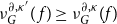



Proof.
Both claims follow from Holley’s criterion ([Reference Grimmett11, Theorem 2.3]). Fix a vertex $v$
and condition on
$v$
and condition on $\{\xi _v \;:\; v \in V \setminus \{v\}\}$
in
$\{\xi _v \;:\; v \in V \setminus \{v\}\}$
in $\mathcal{L} (G,\partial ,\kappa )$
. Now note that
$\mathcal{L} (G,\partial ,\kappa )$
. Now note that $\max \{|\xi _u - \xi _{v}|\;:\; u \sim v\}$
is in
$\max \{|\xi _u - \xi _{v}|\;:\; u \sim v\}$
is in $\{0,1,2\}$
. If it is
$\{0,1,2\}$
. If it is $2$
, then the conditional value at
$2$
, then the conditional value at $v$
is deterministic. If it is
$v$
is deterministic. If it is $1$
, then the height at
$1$
, then the height at $v$
takes two values with equal probability. Finally, if it is
$v$
takes two values with equal probability. Finally, if it is $0$
, then the height at
$0$
, then the height at $v$
takes three values with equal probability. From this observation, it is easy to see that conditioning on
$v$
takes three values with equal probability. From this observation, it is easy to see that conditioning on $\{\xi '_v \;:\; v \in V \setminus \{v\}\}$
with
$\{\xi '_v \;:\; v \in V \setminus \{v\}\}$
with $\xi ' \ge \xi$
stochastically increases the height at
$\xi ' \ge \xi$
stochastically increases the height at $h$
.
$h$
.
A useful tool is monotonicity of the pushforward of the law of $\mathcal{L} (G,\partial ,\kappa )$
under the mapping
$\mathcal{L} (G,\partial ,\kappa )$
under the mapping $h \mapsto |h|$
. Unfortunately it is not true directly as can be seen in the segment graph with three vertices with two vertices having degree one and one having degree 2 (call it
$h \mapsto |h|$
. Unfortunately it is not true directly as can be seen in the segment graph with three vertices with two vertices having degree one and one having degree 2 (call it $v$
). If the the height is
$v$
). If the the height is $0$
on the neighbours of
$0$
on the neighbours of $v$
, then the conditional law of the height at
$v$
, then the conditional law of the height at $v$
is Bernoulli
$v$
is Bernoulli $(2/3)$
. On the other hand, conditioning one of absolute value heights of the neighbours to be 1 makes the conditional law at
$(2/3)$
. On the other hand, conditioning one of absolute value heights of the neighbours to be 1 makes the conditional law at $v$
Bernoulli
$v$
Bernoulli $(1/2)$
.
$(1/2)$
.
It turns out that a different form of absolute value FKG holds, if we do the mapping $h \mapsto |h+0.5|$
. Let
$h \mapsto |h+0.5|$
. Let $\mathcal{L}^{\gt 0}(G,\partial ,\kappa )$
denote the set of
$\mathcal{L}^{\gt 0}(G,\partial ,\kappa )$
denote the set of $1$
-Lipschitz functions taking values in
$1$
-Lipschitz functions taking values in $\mathbb{N} -0.5\,:\!=\, \{0.5,1.5, \ldots \}$
. We also need to be careful with the boundary conditions. We say an admissible boundary condition
$\mathbb{N} -0.5\,:\!=\, \{0.5,1.5, \ldots \}$
. We also need to be careful with the boundary conditions. We say an admissible boundary condition $\kappa$
is
$\kappa$
is $|h|$
-adaptedFootnote
3
if we can break up
$|h|$
-adaptedFootnote
3
if we can break up $\partial$
into
$\partial$
into $\partial = \partial _{\mathrm{pos}} \sqcup \partial _{\mathrm{sym}}$
such that
$\partial = \partial _{\mathrm{pos}} \sqcup \partial _{\mathrm{sym}}$
such that
-
•
$\kappa _v = -\kappa _v$
for every
$v \in \partial _{\mathrm{sym}}$
, -
•
$\kappa _v \subseteq \mathbb{N}+0.5 \,:\!=\, \{1.5,2.5,\ldots \}$
for every
$v \in \partial _{\mathrm{pos}}$
.




For every $\xi \in \mathcal{L}^{\gt 0}(G,\partial ,\kappa )$
, connect two vertices
$\xi \in \mathcal{L}^{\gt 0}(G,\partial ,\kappa )$
, connect two vertices $u,v$
by an edge if
$u,v$
by an edge if $\max \{\xi _u, \xi _v \} \gt 0.5$
. Let
$\max \{\xi _u, \xi _v \} \gt 0.5$
. Let $k(\xi )$
denote the number of connected components which do not intersect
$k(\xi )$
denote the number of connected components which do not intersect $B_{\mathrm{pos}}$
. Then clearly for any
$B_{\mathrm{pos}}$
. Then clearly for any $|h|$
-adapted boundary condition
$|h|$
-adapted boundary condition $\kappa$
,
$\kappa$
,
 \begin{equation} \nu _G^{\partial , \kappa } (|h+0.5| = \xi ) = \frac {2^{k(\xi )}}{|\mathcal{L}(G, \partial , \kappa )|}, \qquad \xi \in \mathcal{L}^{\gt 0}(G, \partial , \kappa ). \end{equation}
Proposition 4.2 (monotonicity for $|h+0.5|$
). Take a finite graph
$|h+0.5|$
). Take a finite graph $G=(V,E)$
with boundary
$G=(V,E)$
with boundary $\partial$
. Let
$\partial$
. Let $\kappa , \kappa '$
be two
$\kappa , \kappa '$
be two $|h|$
-adapted boundary conditions with
$|h|$
-adapted boundary conditions with $\partial _{\mathrm{pos}}(\kappa ) \subseteq \partial _{\mathrm{pos}}(\kappa ')$
and for every
$\partial _{\mathrm{pos}}(\kappa ) \subseteq \partial _{\mathrm{pos}}(\kappa ')$
and for every $v\in \partial$
,
$v\in \partial$
, $[a_v,b_v]\,:\!=\,\kappa _v\cap \{0.5,1.5,\ldots \}$
and
$[a_v,b_v]\,:\!=\,\kappa _v\cap \{0.5,1.5,\ldots \}$
and $[a'_v,b'_v]\,:\!=\,\kappa '_v\cap \{0.5,1.5,\ldots \}$
satisfy
$[a'_v,b'_v]\,:\!=\,\kappa '_v\cap \{0.5,1.5,\ldots \}$
satisfy $a_v\le a'_v$
and
$a_v\le a'_v$
and $b_v\le b'_v$
(these numbers could be
$b_v\le b'_v$
(these numbers could be $\infty$
),
$\infty$
),
-
(CBC) For every increasing function
$f$
,
$\nu ^{\partial , \kappa '}_G[\,f(|h+0.5|)]\ge \nu ^{\partial , \kappa }_G[\,f(|h+0.5|)]$
; -
(FKG) For any two increasing functions
$f,g$
,
$\nu ^ {\partial , \kappa }_G[\,f(|h+0.5|)g(|h+0.5|)] \ge \nu ^ {\partial , \kappa }_G[\,f(|h+0.5|)] \nu ^ {\partial , \kappa }_G[g(|h+0.5|)]$
.




Proof. The proof is very similar to [Reference Duminil-Copin, Harel, Laslier, Raoufi and Ray7, Proposition 2.2].
Fix a vertex $v$
. Using [Reference Georgii, Häggström and Maes10, Theorem 4.8] and references therein, it is sufficient to prove that for any
$v$
. Using [Reference Georgii, Häggström and Maes10, Theorem 4.8] and references therein, it is sufficient to prove that for any $\xi$
(resp.
$\xi$
(resp. $\eta$
) which are restrictions to
$\eta$
) which are restrictions to $V \setminus \{v\}$
of configurations in
$V \setminus \{v\}$
of configurations in $\mathcal{L}^{\gt 0}(G,\partial ,\kappa )$
(resp.
$\mathcal{L}^{\gt 0}(G,\partial ,\kappa )$
(resp. $\mathcal{L}^{\gt 0}(G,\partial ,\kappa ')$
) such that
$\mathcal{L}^{\gt 0}(G,\partial ,\kappa ')$
) such that $\xi _v \le \eta _v$
for all
$\xi _v \le \eta _v$
for all $v$
, and every
$v$
, and every $k \ge 0$
,
$k \ge 0$
,
 \begin{equation} \nu _{G}^{\partial ,\kappa }\big [|h_v+0.5| \ge k\big | |h_{|V\setminus \{v\}}+0.5|= \xi \big ] \le \nu _{G}^{\partial ,\kappa '}\big [|h_v+0.5| \ge k \big | |h+0.5|_{|V\setminus \{v\}}= \eta \big ]. \end{equation}
If $\xi _u \ge 2.5$
for some neighbour
$\xi _u \ge 2.5$
for some neighbour $u$
of
$u$
of $v$
, or if
$v$
, or if $\xi _u = 1.5$
for all neighbours
$\xi _u = 1.5$
for all neighbours $u$
of
$u$
of $v$
, then it is straightforward to see using (4.1) that (4.2) holds, as in this case we are simply reduced to the analysis in Proposition4.1 (the quantity
$v$
, then it is straightforward to see using (4.1) that (4.2) holds, as in this case we are simply reduced to the analysis in Proposition4.1 (the quantity $k(\xi )$
in (4.1) does not change whatever be the value of
$k(\xi )$
in (4.1) does not change whatever be the value of $|h_v+0.5|$
, consequently
$|h_v+0.5|$
, consequently $|h_v+0.5|$
is equally likely among all possibilities dictated by the Lipschitz constraint or the constraint imposed by
$|h_v+0.5|$
is equally likely among all possibilities dictated by the Lipschitz constraint or the constraint imposed by $\kappa , \kappa '$
in case
$\kappa , \kappa '$
in case $v$
is a boundary vertex).
$v$
is a boundary vertex).
Now suppose $\xi _u \le 1.5$
for every neighbour of
$\xi _u \le 1.5$
for every neighbour of $v$
, and
$v$
, and $\xi =0.5$
for at least one of the neighbours of
$\xi =0.5$
for at least one of the neighbours of $v$
(whence
$v$
(whence $|h_v+0.5| \in \{0.5,1.5\}$
). Notice that all the neighbours
$|h_v+0.5| \in \{0.5,1.5\}$
). Notice that all the neighbours $u$
with
$u$
with $\xi _u = 1.5$
must belong to the same component in
$\xi _u = 1.5$
must belong to the same component in $\xi$
, call it
$\xi$
, call it $N_v(\xi )$
. If
$N_v(\xi )$
. If $v \in \partial$
and
$v \in \partial$
and $\{0.5,1.5\} \not \subseteq \kappa _v$
then the value of
$\{0.5,1.5\} \not \subseteq \kappa _v$
then the value of $|h+0.5|$
at
$|h+0.5|$
at $v$
is deterministically equal to
$v$
is deterministically equal to $\kappa _v \cap \{0.5,1.5\}$
. Otherwise, let
$\kappa _v \cap \{0.5,1.5\}$
. Otherwise, let $k'_v(\xi )$
denote the number of components of
$k'_v(\xi )$
denote the number of components of $k(\xi )$
containing at least one of the neighbours
$k(\xi )$
containing at least one of the neighbours $u$
of
$u$
of $v$
with
$v$
with $\xi _u =0.5$
and which do not intersect
$\xi _u =0.5$
and which do not intersect $\partial _{\mathrm{pos}}(\kappa )$
. If
$\partial _{\mathrm{pos}}(\kappa )$
. If $N_v(\xi )$
does not intersect
$N_v(\xi )$
does not intersect $\partial _{\mathrm{pos}}(\kappa )$
, let
$\partial _{\mathrm{pos}}(\kappa )$
, let $k_v(\xi ) = k'_v(\xi )+1$
, otherwise
$k_v(\xi ) = k'_v(\xi )+1$
, otherwise $k_v(\xi ) = k'_v(\xi )$
. Let
$k_v(\xi ) = k'_v(\xi )$
. Let $\mathcal{B}(\kappa )$
denote the event that at least one of the components of
$\mathcal{B}(\kappa )$
denote the event that at least one of the components of $k(\xi )$
containing at least one of the neighbours of
$k(\xi )$
containing at least one of the neighbours of $v$
intersects
$v$
intersects $\partial _{\mathrm{pos}}(\kappa )$
.
$\partial _{\mathrm{pos}}(\kappa )$
.
 \begin{equation*} \nu _{G}^{\partial ,\kappa }\big [|h_v+0.5| =0.5\big | |h+0.5|_{|V\setminus \{v\}}= \xi \big ] = \begin{cases} 0 \text{ if }v \in \partial _{\mathrm{pos}}\\ 2^{k_v(\xi )} /(2 + 2^{k_v(\xi )}) \text{ if $\xi \notin \mathcal{B}(\kappa )$, $v \notin \partial _{\mathrm{pos}}$}\\ 2^{k_v(\xi )} /(1 + 2^{k_v(\xi )})\text{ if $\xi \in \mathcal{B}(\kappa )$, $v \notin \partial _{\mathrm{pos}}$} \end{cases} \end{equation*}
The same formula holds for $\eta$
as well. Now observe that
$\eta$
as well. Now observe that $k_v(\xi ) \ge k_v(\eta )$
since
$k_v(\xi ) \ge k_v(\eta )$
since $\eta _v \ge \xi _v$
for all
$\eta _v \ge \xi _v$
for all $v$
and
$v$
and $\partial _{\mathrm{pos}}(\kappa ) \subseteq \partial _{\mathrm{pos}}(\kappa ')$
. If there is strict inequality
$\partial _{\mathrm{pos}}(\kappa ) \subseteq \partial _{\mathrm{pos}}(\kappa ')$
. If there is strict inequality $k_v(\xi ) \gt k_v(\eta )$
then the above expression for
$k_v(\xi ) \gt k_v(\eta )$
then the above expression for $\xi$
is at least that for
$\xi$
is at least that for $\eta$
in all the cases by monotonicity of
$\eta$
in all the cases by monotonicity of $x \mapsto x/(1+x)$
and
$x \mapsto x/(1+x)$
and $x\mapsto x/(2+x)$
and the fact that
$x\mapsto x/(2+x)$
and the fact that $2^{k}/(2+2^k)\ge 2^{k'}/(1+2^{k'})$
if
$2^{k}/(2+2^k)\ge 2^{k'}/(1+2^{k'})$
if $k\ge k'+1$
. So assume
$k\ge k'+1$
. So assume $k_v(\xi ) = k_v(\eta )$
. If
$k_v(\xi ) = k_v(\eta )$
. If $\xi , \eta$
are both in
$\xi , \eta$
are both in $\mathcal{B}(\kappa )$
or both not in
$\mathcal{B}(\kappa )$
or both not in $\mathcal{B}(\kappa )$
, we are also done for similar reasons. The only case remaining is if
$\mathcal{B}(\kappa )$
, we are also done for similar reasons. The only case remaining is if $\eta \in \mathcal{B}(\kappa ')$
but
$\eta \in \mathcal{B}(\kappa ')$
but $\xi \notin \mathcal{B}(\kappa )$
(recall
$\xi \notin \mathcal{B}(\kappa )$
(recall $\mathcal{B}(\kappa ) \subseteq \mathcal{B}(\kappa ')$
) and
$\mathcal{B}(\kappa ) \subseteq \mathcal{B}(\kappa ')$
) and $k_v(\xi ) = k_v(\eta )$
. We claim that this is impossible, as in this case the strict inequality
$k_v(\xi ) = k_v(\eta )$
. We claim that this is impossible, as in this case the strict inequality $k_v(\xi ) \gt k_v(\eta )$
must hold. Indeed, in this case there must be a neighbour of
$k_v(\xi ) \gt k_v(\eta )$
must hold. Indeed, in this case there must be a neighbour of $v$
whose cluster intersects
$v$
whose cluster intersects $B_{\mathrm{pos}}(\kappa ')$
and is not counted in
$B_{\mathrm{pos}}(\kappa ')$
and is not counted in $k_v(\eta )$
, but every neighbour cluster is counted in
$k_v(\eta )$
, but every neighbour cluster is counted in $\xi$
as none of them intersect
$\xi$
as none of them intersect $B_{\mathrm{pos}}(\kappa )$
on the event
$B_{\mathrm{pos}}(\kappa )$
on the event $\mathcal{B}(\kappa )$
.
$\mathcal{B}(\kappa )$
.
Corollary 4.3.
Let $G$
be an infinite graph with a fixed vertex
$G$
be an infinite graph with a fixed vertex $\rho$
. Let
$\rho$
. Let $(G_k)_{k \ge 1}$
be a sequence such that
$(G_k)_{k \ge 1}$
be a sequence such that $G_k \subseteq G_{k+1}$
and
$G_k \subseteq G_{k+1}$
and $\cup G_k = G$
. Suppose
$\cup G_k = G$
. Suppose $\partial _k$
be a subset of vertices of
$\partial _k$
be a subset of vertices of $G_k$
such that
$G_k$
such that $\partial _{k+1} \cap G_k \subseteq \partial _k$
, and the distance between
$\partial _{k+1} \cap G_k \subseteq \partial _k$
, and the distance between $\partial _k$
and
$\partial _k$
and $\rho$
converges to
$\rho$
converges to $\infty$
. Let
$\infty$
. Let $\kappa ^k_v = \{-0.5,0.5\}$
for all
$\kappa ^k_v = \{-0.5,0.5\}$
for all $v \in \partial _k$
. Then one of the following two cases hold.
$v \in \partial _k$
. Then one of the following two cases hold. $(\mathbf{Localization})$ $\nu ^{G_k}_{\partial _k, \kappa ^k}$
converges to a translation-invariant Gibbs measure supported on Lipschitz functions on
$\nu ^{G_k}_{\partial _k, \kappa ^k}$
converges to a translation-invariant Gibbs measure supported on Lipschitz functions on $G$
.
$G$
. $(\mathbf{Delocalization})$ $\lim _{m \to \infty } \sup _{k }\mu ^{G_k}_{\partial _k, \kappa ^k}(|h(\rho )| \gt m) \gt 0$
.
$\lim _{m \to \infty } \sup _{k }\mu ^{G_k}_{\partial _k, \kappa ^k}(|h(\rho )| \gt m) \gt 0$
.
Proof.
Let $h^k \sim \mu ^{G_k}_{\partial _k, \kappa ^k}$
. Observe that
$h^k \sim \mu ^{G_k}_{\partial _k, \kappa ^k}$
. Observe that $|h^n+0.5|$
is stochastically increasing in
$|h^n+0.5|$
is stochastically increasing in $k$
, and hence if the delocalization condition does not hold,
$k$
, and hence if the delocalization condition does not hold, $\{|h^k+0.5|\}_{k \ge 1}$
is tight. Consequently, weak limit of
$\{|h^k+0.5|\}_{k \ge 1}$
is tight. Consequently, weak limit of $|h^k+0.5|$
exists as a probability measure on
$|h^k+0.5|$
exists as a probability measure on $\mathbb{Z}^V$
. Furthermore, observe that for each
$\mathbb{Z}^V$
. Furthermore, observe that for each $k$
, the height function
$k$
, the height function $h^k+0.5$
is obtained by assigning a uniformly random sign to each connected component of
$h^k+0.5$
is obtained by assigning a uniformly random sign to each connected component of $\xi$
as described in Equation (4.1). Thus, this rule to obtain the height function from the absolute value also persists in the weak limit, and the proof of the corollary is complete.
$\xi$
as described in Equation (4.1). Thus, this rule to obtain the height function from the absolute value also persists in the weak limit, and the proof of the corollary is complete.
Proof of Theorem
1.2. Using Proposition4.1, $\mu _{k,d}^{\{0,1\}}$
is dominated by
$\mu _{k,d}^{\{0,1\}}$
is dominated by $\mu _{k,d}^{1}$
and dominates
$\mu _{k,d}^{1}$
and dominates $\mu _{k,d}^{0}$
, both of which are tight by Theorem1.1. Thus
$\mu _{k,d}^{0}$
, both of which are tight by Theorem1.1. Thus $\mu _{k,d}^{\{0,1\}}$
is tight. Thus
$\mu _{k,d}^{\{0,1\}}$
is tight. Thus $\mu _{k,d}^{\{0,1\}}$
is in the localization phase of Corollary4.3, and the result follows.
$\mu _{k,d}^{\{0,1\}}$
is in the localization phase of Corollary4.3, and the result follows.
5. Discussion and open questions
In this section, we briefly discuss some properties of the limiting measures $\mu ^{S}_{d}$
for finite subsets
$\mu ^{S}_{d}$
for finite subsets $S \subset \mathbb{Z}$
. Let us first show how to construct translation-invariant Gibbs measures on
$S \subset \mathbb{Z}$
. Let us first show how to construct translation-invariant Gibbs measures on $d$
-regular trees rather than
$d$
-regular trees rather than $d$
-ary trees, the nice thing about the former is that they are vertex transitive. The convergence result for the
$d$
-ary trees, the nice thing about the former is that they are vertex transitive. The convergence result for the $d$
-regular tree actually follows from that of the
$d$
-regular tree actually follows from that of the $d$
-ary tree in a straightforward manner: Let
$d$
-ary tree in a straightforward manner: Let $ f_k \sim \mu ^S_{d,k}$
, and let
$ f_k \sim \mu ^S_{d,k}$
, and let $\tilde f_k \sim \tilde \mu ^S_{d,k}$
denote the analogous law for the
$\tilde f_k \sim \tilde \mu ^S_{d,k}$
denote the analogous law for the $d+1$
-regular tree. Then
$d+1$
-regular tree. Then
 \begin{equation*} \mathbb{P}(\tilde f_k(\rho ) = i) = F_{d+1}(F_d^{(k-1)} (\delta _S))_i \end{equation*}
where $F_d$
is the map
$F_d$
is the map $F$
for
$F$
for $d$
-ary tree as described in the beginning of Section 2. Thus the limit as
$d$
-ary tree as described in the beginning of Section 2. Thus the limit as $k \to \infty$
for the
$k \to \infty$
for the $d+1$
-regular tree exists whenever it exists for the
$d+1$
-regular tree exists whenever it exists for the $d$
-ary tree. Furthermore if
$d$
-ary tree. Furthermore if $\pi ^S_d\,:\!=\,\pi ^S_d(\rho )$
denote the law of the height at
$\pi ^S_d\,:\!=\,\pi ^S_d(\rho )$
denote the law of the height at $\rho$
under
$\rho$
under $\mu ^{S}_d$
, whenever it exists, then the corresponding law for the
$\mu ^{S}_d$
, whenever it exists, then the corresponding law for the $d+1$
-regular tree is given by
$d+1$
-regular tree is given by $F_{d+1}(\pi _d^S)$
. It is also easy to check that the transition matrix for the tree indexed Markov chain for the
$F_{d+1}(\pi _d^S)$
. It is also easy to check that the transition matrix for the tree indexed Markov chain for the $d$
-ary tree as well as the
$d$
-ary tree as well as the $d+1$
regular tree is given by
$d+1$
regular tree is given by
 \begin{equation*} (P^S_d)_{i,j} = \frac {\pi _d^S(j)}{\pi _d^S(i-1)+\pi _d^S(i)+\pi _d^S(i+1)}1_{|j-i|\le 1}. \end{equation*}
and that $F_{d+1}(\pi ^S_d)$
is the stationary measure for this transition matrix. Using reversibility of the chain, translation invariance of the limit for the
$F_{d+1}(\pi ^S_d)$
is the stationary measure for this transition matrix. Using reversibility of the chain, translation invariance of the limit for the $d+1$
-regular tree is immediate.
$d+1$
-regular tree is immediate.
We now speculate about the most general result possible for general boundary conditions in our setup. We saw that for small $d$
convergence holds for all the cases we considered here. For large
$d$
convergence holds for all the cases we considered here. For large $d$
, however, such convergence holds along the even sequences. This leads us to conjecture:
$d$
, however, such convergence holds along the even sequences. This leads us to conjecture:
Conjecture 5.1. $\lim _{k \to \infty }\mu _{k,2}^S$
exists for all finite
$\lim _{k \to \infty }\mu _{k,2}^S$
exists for all finite $S$
. Also,
$S$
. Also, $\lim _{k \to \infty }\mu _{2k,d}^S$
exists for all finite
$\lim _{k \to \infty }\mu _{2k,d}^S$
exists for all finite $S$
and for all
$S$
and for all $d \ge 2$
.
$d \ge 2$
.
We believe that for $S = \{-N,\ldots , N\}$
and
$S = \{-N,\ldots , N\}$
and $d \ge 8$
, a more careful analysis similar to that in Section 6 should be enough to conclude the convergence of the map
$d \ge 8$
, a more careful analysis similar to that in Section 6 should be enough to conclude the convergence of the map $\psi \circ \psi$
.
$\psi \circ \psi$
.
Next comes the question of understanding all possible translation-invariant measures we can get as limits of the above type. To summarize the results of this article, we constructed the translation-invariant Gibbs measures $\tilde \mu _d^{S}$
,
$\tilde \mu _d^{S}$
, $S = \{-N,\ldots , N\}$
for
$S = \{-N,\ldots , N\}$
for $2 \le d \le 7$
and for
$2 \le d \le 7$
and for $S=\{0,1\}$
,
$S=\{0,1\}$
, $d \ge 2$
. We also proved that for
$d \ge 2$
. We also proved that for $2 \le d \le 7$
,
$2 \le d \le 7$
, $\tilde \mu _d^{\{0,1\}} \neq \tilde \mu _d^0 = \tilde \mu _d^{\{-N,\ldots , N\}}$
for all
$\tilde \mu _d^{\{0,1\}} \neq \tilde \mu _d^0 = \tilde \mu _d^{\{-N,\ldots , N\}}$
for all $N \ge 0$
. This raised the following research programme.
$N \ge 0$
. This raised the following research programme.
Question 5.2.
Characterize all translation-invariant measures of the form $\tilde \mu _d^S$
where
$\tilde \mu _d^S$
where $S \subset \mathbb{Z}$
is finite, whenever they exist. In particular, is there a natural set of properties such that if
$S \subset \mathbb{Z}$
is finite, whenever they exist. In particular, is there a natural set of properties such that if $S_1,S_2$
satisfies all of the properties, then it is guaranteed that
$S_1,S_2$
satisfies all of the properties, then it is guaranteed that $\tilde \mu _d^{S_1} = \tilde \mu _d^{S_2}\, ?$
Another interesting direction is to consider $M$
-Lipschitz functions for
$M$
-Lipschitz functions for $M\gt 1$
.
$M\gt 1$
.
Question 5.3.
Extend Theorem
1.2
to $M\gt 1$
: Does
$M\gt 1$
: Does $\mu ^{\{0,\dots ,M\}}_{k,d,M}$
converge for all
$\mu ^{\{0,\dots ,M\}}_{k,d,M}$
converge for all $d \ge 2$
and
$d \ge 2$
and $M \ge 2\, ?$
Question 5.4.
Extend Theorem
1.1
to $M\gt 1$
: Given
$M\gt 1$
: Given $M\gt 1$
, show that
$M\gt 1$
, show that $\mu ^0_{k,d,M}$
converges if and only if
$\mu ^0_{k,d,M}$
converges if and only if $d \le d_c(M)$
. Can one at least show convergence for
$d \le d_c(M)$
. Can one at least show convergence for $M \gg d \, ?$
Another very interesting avenue of research is extremality. The measures $\tilde \mu _d^{0}$
and
$\tilde \mu _d^{0}$
and $\tilde \mu _d^{\{0,1\}}$
are both mixing, hence ergodic. However, the question of whether they are extremal remains:
$\tilde \mu _d^{\{0,1\}}$
are both mixing, hence ergodic. However, the question of whether they are extremal remains:
Question 5.5.
For what values of $d$
are the measures
$d$
are the measures $\mu _d^{\{0,1\}}$
and
$\mu _d^{\{0,1\}}$
and $\mu _{d}^0$
extremal for
$\mu _{d}^0$
extremal for $2 \le d \le 7 \, ?$
This is related to the question of extremality of the Ising model, see [Reference Lyons19, Section 3].
6. Estimates of fixed point of
$\varphi$

In this section, we complete the proof of Proposition2.8. Recall from Lemma2.2 that
 \begin{equation*} \psi (\mathcal{S}_{a,b,c}) \subset \mathcal{S}_{a',b',c'}, \end{equation*}
where
 \begin{align*} (a',b',c')= \varphi (a,b,c) \,:\!=\, (f(1,b), f(1+c,a), g(b,c)) , \end{align*}
and
 \begin{align*} f(\alpha ,x) &\,:\!=\, \left (\frac {1+\alpha x}{1+2x}\right )^d, \\ g(b,x) &\,:\!=\, b^d \left (\frac {1+x+x^2}{1+b+bx}\right )^d. \end{align*}
Let us summarize the basic strategy to approximate the fixed point of $\varphi$
.
$\varphi$
.
-
• First we prove in Lemma6.1 that
$x \mapsto g(b,x)$
has a unique fixed point in
$(0,1)$
. -
• Since
$\mathcal{S}_{\varphi (0,1,c)} \subset \mathcal{S}_{0,1,g(1,c)}$
, we can iterate this bound many times to reach close to
$\mathcal{S}_{0,1,c_g}$
where
$c_g$
is the unique fixed point of
$x\mapsto g(1,x)$
in
$(0,1)$
. -
• Next we note that
where
\begin{equation*}\psi \circ \psi (\mathcal{S}_{a,b,c_g})) \subset \mathcal{S}_{\mathsf{i}(c_g,a), \mathsf{j}(c_g,a), c_g}\end{equation*}
$\mathsf{i}, \mathsf{j}$
are defined as in (6.1). The reason for this approximation is that now it is enough to analyse the one dimensional maps
$\mathsf{i}, \mathsf{j}$
(with
$c_g$
fixed).
-
• We prove in Lemma6.3 next that
$\mathsf{i}, \mathsf{j}$
have derivatives in
$(0,1)$
which (along with some other basic properties) is enough to prove that each of them has a unique fixed point in
$(0,1)$
. We call them
$a_{c_g}, b_{c_g}$
. In conclusion, after enough iterates we approximately reach
$\mathcal{S}_{a_{c_g}, b_{c_g}, c_g}$
. -
• It turns out that
$a_{c_g}, b_{c_g}, c_g$
can be taken to be our estimates
$\hat a_*, \hat b_*, \hat c_*$
for
$3 \le d \le 6$
. Unfortunately for
$d=2,7$
, these estimates are not enough. For these two cases we need another ‘round’ of approximation as follows. -
• In Lemma6.5, we prove using similar ideas that starting close to
$\mathcal{S}_{a_{c_g}, b_{c_g}, c_g}$
, we can reach
$\mathcal{S}_{a_{c_g}, b_{c_g}, \tilde c_g}$
where
$\tilde c_g$
is the unique fixed point of
$x\mapsto g(b_g',x)$
where
$b_g'=\max\! (f(1+c_g,a_{c_g}), b_g)$
. -
• Finally, in Lemma6.6, we prove that starting close to
$\mathcal{S}_{a_{c_g}, b_{c_g}, \tilde c_g}$
we reach
$\mathcal{S}_{a_{\tilde c_g}, b_{\tilde c_g}, \tilde c_g}$
where
$a_{\tilde c_g}, b_{\tilde c_g}$
are unique fixed points of
$x \mapsto \mathsf{i}(x,\tilde c_g), x\mapsto \mathsf{j}(x, \tilde c_g)$
. -
• Now we need to explain how we get hold of the values close enough to the fixed points
$c_g, a_{c_g}, b_{c_g}, \tilde c_g, a_{\tilde c_g}, b_{\tilde c_g}$
. We prove in Lemma6.2 that the map
$x \gt g(b,x)$
if and only if
$x \lt c_g$
where
$c_g$
is the fixed point of
$x \mapsto g(b,x)$
. Thus if we can produce two points
$c_1, c_2$
such that
$g(b,c_1) \gt c_1$
and
$g(b,c_2)\lt c_2$
then
$c_1\lt c_g\lt c_2$
. In practice, we can ‘guess’ good estimates of
$c_1,c_2$
by looking at the plots and then plug them into
$g(b,x)$
to confirm that indeed
$g(b,c_1)\gt c_1$
,
$g(b,c_2)\lt c_2$
, which makes the estimates completely rigorous. The maps
$x \mapsto \mathsf{i}(c,x), x \mapsto \mathsf{j}(c,x)$
also satisfy similar properties which we exploit in a similar manner to get good estimates of
$a_{c_g}, b_{c_g}$
and then
$a_{\tilde c_g}, b_{\tilde c_g}$
. This part is done in a separate subsection Section 6.1.















We now explain the details of the above strategy.
Lemma 6.1.
For $x\gt 0,b\in (0,1]$
,
$x\gt 0,b\in (0,1]$
, $x \mapsto g(b,x)$
is increasing, convex and has a unique fixed point
$x \mapsto g(b,x)$
is increasing, convex and has a unique fixed point $c_0$
in
$c_0$
in $(0,1)$
. Moreover, if
$(0,1)$
. Moreover, if $0 \le c\lt 1$
then for any fixed
$0 \le c\lt 1$
then for any fixed $b$
, defining
$b$
, defining $g_b(c) = g(b,c)$
,
$g_b(c) = g(b,c)$
, $g_b^{(i)}(c)$
converges to
$g_b^{(i)}(c)$
converges to $c_0 = c_0(b)$
. Also,
$c_0 = c_0(b)$
. Also, $g_b(x)\gt x$
if and only if
$g_b(x)\gt x$
if and only if $x\lt c_0(b)$
.
$x\lt c_0(b)$
.
Proof. We have
 \begin{equation*} \frac {\partial g}{\partial x} = \frac {db^d(bx^2+2bx+2x+1)(x^2+x+1)^{d-1}}{(bx+b+1)^{d+1}} \end{equation*}
and
 \begin{align*} &\frac {\partial ^2 g}{\partial x^2} = d b^d (x^2 + x + 1)^{d - 2} (b x + b + 1)^{-d - 2}\\ &(b^2 ((d - 1) x^4 + 4 (d - 1) x^3 + (4 d - 2) x^2 + 2 x + 2) + 2 b (2 (d - 1) x^3 + (5 d - 4) x^2\\ &\quad + (2 d - 1) x + 1) + d (2 x + 1)^2 - 2 x^2 - 2 x + 1) \end{align*}
It can be easily checked from these expressions that $\partial g/\partial x$
and
$\partial g/\partial x$
and $\partial ^2g/\partial x^2$
are both strictly positive for
$\partial ^2g/\partial x^2$
are both strictly positive for $d \ge 2$
.
$d \ge 2$
.
For $b\lt 1$
, since
$b\lt 1$
, since $g(b,0) = b^d \gt 0$
and
$g(b,0) = b^d \gt 0$
and $g(b,1) \lt g(1,1) = 1$
and
$g(b,1) \lt g(1,1) = 1$
and $g$
is strictly increasing and convex, it must be the case that
$g$
is strictly increasing and convex, it must be the case that $g$
has a unique fixed point in
$g$
has a unique fixed point in $(0,1)$
. If
$(0,1)$
. If $b=1$
, although
$b=1$
, although $g(1)=1$
, and we further note that
$g(1)=1$
, and we further note that
 \begin{equation*}\frac {\partial g}{\partial x}|_{x=1} = \frac {2d}{3}\gt 1\end{equation*}
if $d \ge 2$
. Thus
$d \ge 2$
. Thus $g$
has a unique fixed point in
$g$
has a unique fixed point in $(0,1)$
in this case also. This takes care of the ‘also’ part in the lemma as well.
$(0,1)$
in this case also. This takes care of the ‘also’ part in the lemma as well.
The fact that $g^{(i)}(c)$
converges to the fixed point
$g^{(i)}(c)$
converges to the fixed point $c_0$
is immediate from the fact that
$c_0$
is immediate from the fact that $c_0\lt g(x)\lt x$
if
$c_0\lt g(x)\lt x$
if $x\gt c_0$
and
$x\gt c_0$
and $c_0\gt g(x)\gt x$
if
$c_0\gt g(x)\gt x$
if $x\lt c_0$
, and hence the iterates monotonically converge to
$x\lt c_0$
, and hence the iterates monotonically converge to $c_0$
.
$c_0$
.
We now introduce a convenient notion of convergence of sets of the form $\mathcal{S}_{a,b,c}$
. We say
$\mathcal{S}_{a,b,c}$
. We say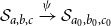 $\mathcal{S}_{a,b,c} \xrightarrow []{\psi } \mathcal{S}_{a_0,b_0,c_0}$
if for all
$\mathcal{S}_{a,b,c} \xrightarrow []{\psi } \mathcal{S}_{a_0,b_0,c_0}$
if for all $x \in \mathcal{S}_{a,b,c}$
and all
$x \in \mathcal{S}_{a,b,c}$
and all $\varepsilon \gt 0$
, there exists a
$\varepsilon \gt 0$
, there exists a $K$
such that for all
$K$
such that for all $k \ge K$
,
$k \ge K$
, $\psi ^{(k)}(x) \in \mathcal{S}_{a_0-\varepsilon ,b_0+\varepsilon ,c_0+\varepsilon }$
. Similarly, we define
$\psi ^{(k)}(x) \in \mathcal{S}_{a_0-\varepsilon ,b_0+\varepsilon ,c_0+\varepsilon }$
. Similarly, we define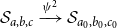 $\mathcal{S}_{a,b,c} \xrightarrow []{\psi ^2} \mathcal{S}_{a_0,b_0,c_0}$
for all
$\mathcal{S}_{a,b,c} \xrightarrow []{\psi ^2} \mathcal{S}_{a_0,b_0,c_0}$
for all $x \in \mathcal{S}_{a,b,c}$
and all
$x \in \mathcal{S}_{a,b,c}$
and all $\varepsilon \gt 0$
, there exists a
$\varepsilon \gt 0$
, there exists a $K$
such that for all
$K$
such that for all $k \ge K$
,
$k \ge K$
, $\psi ^{(2k)}(x) \in \mathcal{S}_{a_0-\varepsilon ,b_0+\varepsilon ,c_0+\varepsilon }$
.
$\psi ^{(2k)}(x) \in \mathcal{S}_{a_0-\varepsilon ,b_0+\varepsilon ,c_0+\varepsilon }$
.
Lemma 6.2.
Fix $c\lt 1$
. We have
$c\lt 1$
. We have
 \begin{equation*}\mathcal{S}_{0,1,c} \xrightarrow []{\psi } \mathcal{S}_{0,1,c_g},\end{equation*}
where $c_g$
is the unique fixed point of
$c_g$
is the unique fixed point of $g(1,\cdot )$
in
$g(1,\cdot )$
in $(0,1)$
(as guaranteed by Lemma
6.1
).
$(0,1)$
(as guaranteed by Lemma
6.1
).
Now we plan to bootstrap this estimate into an iteration of the first two coordinates. To that end, define
 \begin{equation} \mathsf{i}(c,x) \,:\!=\, f(1,f(1+c,x)), \qquad \mathsf{j}(c,x) \,:\!=\, f(1+c, f(1,x)). \end{equation}
To motivate these definitions, note that $\mathsf{i}(c,a)$
is precisely the first coordinate of
$\mathsf{i}(c,a)$
is precisely the first coordinate of $\varphi ^{(2)}(a,b,c)$
. It turns out that
$\varphi ^{(2)}(a,b,c)$
. It turns out that $\mathsf{ j}(c,b)$
serves as a bound on the second coordinate of
$\mathsf{ j}(c,b)$
serves as a bound on the second coordinate of $\varphi ^{(2)}(a,b,c)$
when
$\varphi ^{(2)}(a,b,c)$
when $c=c_g$
.
$c=c_g$
.
Lemma 6.3.
For all $2 \le d \le 7$
, there exists a
$2 \le d \le 7$
, there exists a $0\lt c_g\lt c_d$
such that for all
$0\lt c_g\lt c_d$
such that for all $c\lt c_d$
, both
$c\lt c_d$
, both $x \mapsto \mathsf{i}(c,x)$
and
$x \mapsto \mathsf{i}(c,x)$
and $x \mapsto \mathsf{ j}(c,x)$
have unique fixed points
$x \mapsto \mathsf{ j}(c,x)$
have unique fixed points $a_{ c},b_{c}$
in
$a_{ c},b_{c}$
in $(0,1)$
. Furthermore, both
$(0,1)$
. Furthermore, both $|\partial \mathsf{i}/\partial x |\lt 1$
and
$|\partial \mathsf{i}/\partial x |\lt 1$
and $|\partial \mathsf{ j}/\partial x |\lt 1$
in
$|\partial \mathsf{ j}/\partial x |\lt 1$
in $[0,1]$
. Consequently for any
$[0,1]$
. Consequently for any $x \in [0,1]$
,
$x \in [0,1]$
,
 \begin{equation*}\mathsf{i}^{(k)}(x) \to a_{c} \text{ and }\mathsf{j}^{(k)}(x) \to b_{c}\text{ as } k \to \infty .\end{equation*}
Furthermore, $\mathsf{i}(c,x)\gt x$
if and only if
$\mathsf{i}(c,x)\gt x$
if and only if $x \in [0,a_c)$
and
$x \in [0,a_c)$
and $\mathsf{j}(c,x)\gt x$
if and only if
$\mathsf{j}(c,x)\gt x$
if and only if $x \in [0,b_c)$
.
$x \in [0,b_c)$
.
We postpone the proof of Lemma6.3 to later in order to maintain the flow of the argument.
Lemma 6.4.
Let $c_g$
be as in Lemma
6.2
and
$c_g$
be as in Lemma
6.2
and $a_{c_g},b_{c_g}$
as in Lemma
6.3
for
$a_{c_g},b_{c_g}$
as in Lemma
6.3
for $c=c_g$
. Then for all
$c=c_g$
. Then for all $c\lt 1$
 \begin{equation*} \mathcal{S}_{0,1,c} \xrightarrow []{\psi ^2} \mathcal{S}_{a_{c_g}, b_{c_g}, c_g}. \end{equation*}
as $k \to \infty$
.
$k \to \infty$
.
Proof.
Applying Lemma6.2, we see that for all $\delta \ge 0$
so that
$\delta \ge 0$
so that $c_g+\delta \lt 1$
for all large enough
$c_g+\delta \lt 1$
for all large enough $k$
$k$
 \begin{equation*} \psi ^{(k)} (\mathcal{S}_{0,1,c} ) \subset \mathcal{S}_{0,1,c_g+\delta } \end{equation*}
Recall
 \begin{equation*} \varphi (a,b,c_g+\delta ) = (f(1,b), f(1+c_g+\delta ,a), g(b,c_g+\delta )) \end{equation*}
Since $g(b,x)$
is increasing in
$g(b,x)$
is increasing in $b$
, and
$b$
, and $g(1,x)\le x$
if and only if
$g(1,x)\le x$
if and only if $x \ge c_g$
,
$x \ge c_g$
, $g(b,c_g+\delta ) \le g(1,c_g+\delta ) \le c_g+\delta$
. Thus we have
$g(b,c_g+\delta ) \le g(1,c_g+\delta ) \le c_g+\delta$
. Thus we have
 \begin{equation*} \mathcal{S}_{\varphi (a,b,c_g+\delta )} \subseteq \mathcal{S}_{f(1,b), f(1+c_g+\delta ,a), c_g+\delta } \end{equation*}
Now note
 \begin{align*} &\varphi (f(1,b), f(1+c_g+\delta ,a), c_g+\delta )\\ & \quad = (f(1,f(1+c_g+\delta ,a)), f(1+c_g+\delta , f(1,b)), g(f(1+c_g,a), c_g+\delta )). \end{align*}
Note again that $g(f(1+c_g,a), c_g+\delta ) \le g(1,c_g+\delta ) \le c_g+\delta$
. Thus we get
$g(f(1+c_g,a), c_g+\delta ) \le g(1,c_g+\delta ) \le c_g+\delta$
. Thus we get
 \begin{equation*} \mathcal{S}_{\varphi (f(1,b), f(1+c_g+\delta ,a), c_g+\delta )} \subset \mathcal{S}_{\mathsf{i}(c_g+\delta ,a),\mathsf{j}(c_g+\delta ,b), c_g+\delta }. \end{equation*}
Overall
 \begin{align*} &\psi \circ \psi (\mathcal{S}_{a,b,c_g+\delta }) \subset \psi (\mathcal{S}_{\varphi (a,b,c_g+\delta )}) \subset \psi (\mathcal{S}_{f(1,b), f(1+c_g+\delta ,a), c_g})\\ &\quad\subset \mathcal{S}_{\varphi (f(1,b), f(1+c_g+\delta ,a), c_g+\delta )} \subset \mathcal{S}_{\mathsf{i}(c_g+\delta ,a),\mathsf{j}(c_g+\delta ,b), c_g+\delta }. \end{align*}
Thus iterating, and using Lemma6.3, eventually the sequence enters $\mathcal{S}_{a_{c_g(\delta )}-\varepsilon , b_{c_g(\delta )}+\varepsilon , c_g+\delta }$
for arbitrarily small
$\mathcal{S}_{a_{c_g(\delta )}-\varepsilon , b_{c_g(\delta )}+\varepsilon , c_g+\delta }$
for arbitrarily small $\varepsilon$
, where
$\varepsilon$
, where $a_{c_g(\delta )} ,b_{c_g(\delta )}$
are the unique fixed points of
$a_{c_g(\delta )} ,b_{c_g(\delta )}$
are the unique fixed points of $x \mapsto \mathsf{i}(c_g+\delta , x)$
and
$x \mapsto \mathsf{i}(c_g+\delta , x)$
and $\mathsf{j}(c_g+\delta , x)$
in
$\mathsf{j}(c_g+\delta , x)$
in $(0,1)$
respectively. By continuity,
$(0,1)$
respectively. By continuity, $a_{c_g(\delta )} \to a_{c_g}, b_{c_g(\delta )} \to b_{c_g}$
as
$a_{c_g(\delta )} \to a_{c_g}, b_{c_g(\delta )} \to b_{c_g}$
as $\delta \to 0$
. This allows us to conclude the lemma.
$\delta \to 0$
. This allows us to conclude the lemma.
Although the approximation $(a_{c_g},b_{c_g}, c_g)$
for the fixed point of
$(a_{c_g},b_{c_g}, c_g)$
for the fixed point of $\varphi (a,b,c)$
is good enough for
$\varphi (a,b,c)$
is good enough for $3 \le d \le 6$
, we need another round of iteration to get closer to the fixed point of
$3 \le d \le 6$
, we need another round of iteration to get closer to the fixed point of $\varphi (a,b,c)$
for
$\varphi (a,b,c)$
for $d \in \{2,7\}$
. To that end, define
$d \in \{2,7\}$
. To that end, define
 \begin{equation*}b_g' = \max\! (f(1+c_g,a_{c_g}), b_{c_g}).\end{equation*}
Let $\tilde c_g$
be the fixed point of the map
$\tilde c_g$
be the fixed point of the map $x \mapsto g(b_g', x)$
(which is guaranteed to exist by Lemma6.2).
$x \mapsto g(b_g', x)$
(which is guaranteed to exist by Lemma6.2).
Lemma 6.5.
We have for all $c\lt 1$
 \begin{equation*} \mathcal{S}_{0, 1, c} \xrightarrow []{\psi ^2} \mathcal{S}_{a_{c_g}, b_{c_g}, \tilde c_g} \end{equation*}
as $k \to \infty$
. Furthermore,
$k \to \infty$
. Furthermore, $\tilde c_g \lt c_g\lt c_d$
.
$\tilde c_g \lt c_g\lt c_d$
.
Proof.
Since $b_g' \lt 1$
,
$b_g' \lt 1$
, $\tilde c_g = g(b_g',\tilde c_g) \lt g(1, \tilde c_g)$
which implies
$\tilde c_g = g(b_g',\tilde c_g) \lt g(1, \tilde c_g)$
which implies $\tilde c_g\lt c_g$
.
$\tilde c_g\lt c_g$
.
Next, by Lemma6.4, for all $\delta$
,
$\delta$
,
 \begin{equation*} \psi ^{(2k)} (\mathcal{S}_{0,1,c}) \subset \mathcal{S}_{a_{c_g} - \delta , b_{c_g} + \delta , c_g+\delta }. \end{equation*}
for all large enough $k$
. Pick
$k$
. Pick $\delta$
small enough so that
$\delta$
small enough so that $c_g+\delta \lt c_d$
and
$c_g+\delta \lt c_d$
and $b_g''\lt 1$
where
$b_g''\lt 1$
where
 \begin{equation} b_g'' = \max\! (f(1+c_g+\delta ,a_{c_g } -\delta ), b_{c_g} + \delta ). \end{equation}
Note that
 \begin{equation*} g(b_g'',c_g ) \lt g(1,c_g) = c_g \end{equation*}
Hence by continuity we can pick a further small $\delta$
if required to conclude that
$\delta$
if required to conclude that $g(b_g'', c_g+\delta ) \le c_g$
.
$g(b_g'', c_g+\delta ) \le c_g$
.
We first show that after two more steps of iteration, we enter $\mathcal{S}_{a_{c_g} - \delta , b_{c_g} + \delta , c_g}$
. Indeed after one iteration
$\mathcal{S}_{a_{c_g} - \delta , b_{c_g} + \delta , c_g}$
. Indeed after one iteration
 \begin{equation*} \psi (\mathcal{S}_{a_{c_g} - \delta , b_{c_g} + \delta , c_g}) \subset \mathcal{S}_{f(1,b_{c_g}+\delta ),f(1+c_g+\delta , a_{c_g} - \delta ) ,g(b_{c_g-\delta },c_g)} \end{equation*}
by the choice of $k$
. Now note since
$k$
. Now note since $b \mapsto g(b,x)$
is increasing in
$b \mapsto g(b,x)$
is increasing in $b$
,
$b$
,
 \begin{equation*} g(b_{c_g-\delta }, c_g+\delta ) \le g(b_g'', c_g+\delta ) \le c_g \end{equation*}
by the choice of $\delta$
. By the same logic and the choice of
$\delta$
. By the same logic and the choice of $k$
, after another iteration, we are in
$k$
, after another iteration, we are in $\mathcal{S}_{a_{c_g} - \delta , b_{c_g} + \delta , c_g}$
.
$\mathcal{S}_{a_{c_g} - \delta , b_{c_g} + \delta , c_g}$
.
We will show that for all $c\le c_g$
,
$c\le c_g$
,
 \begin{equation} \psi ^{(2)}\big(\mathcal{S}_{a_{c_g}-\delta ,b_{c_g}+\delta ,c}\big) \subseteq \mathcal{S}_{a_{c_g}-\delta , b_{c_g}+\delta , g(b_g'',g(b_g'',c))} \text{ and } g\big(b_g'',g(b_g'',c)\big) \le c_g. \end{equation}
Indeed by Lemma6.2, this is enough since the fixed point of $x \mapsto g(b_g'',x)$
tends to that of
$x \mapsto g(b_g'',x)$
tends to that of $x \mapsto g(b_g',x)$
as
$x \mapsto g(b_g',x)$
as $\delta \to 0$
by continuity.
$\delta \to 0$
by continuity.
Since $b \mapsto g(b,x)$
is increasing (see (2.6)) and
$b \mapsto g(b,x)$
is increasing (see (2.6)) and $c \mapsto f(1+c,x)$
is increasing,
$c \mapsto f(1+c,x)$
is increasing,
 \begin{equation*} g(b_{c_g}+\delta , c) \le g(b_g'',c), \qquad \qquad f(1+c, a_{c_g}-\delta ) \le f(1+c_g, a_{c_g}-\delta ). \end{equation*}
Thus we have
 \begin{equation*} \mathcal{S}_{\varphi (a_{c_g}-\delta , b_{c_g}+\delta ,c)} \subseteq \mathcal{S}_{f(1,b_{c_g}+\delta ), f(1+c_g,a_{c_g}-\delta ), g(b_g'',c)}. \end{equation*}
Now
 \begin{align*} &\varphi (f(1,b_{c_g}+\delta ), f(1+c_g,a_{c_g}-\delta ), g(b_g'',c)) \\ & \quad = (f(1,f(1+c_g,a_{c_g}-\delta )), f(1+g(b_g'',c), f(1,b_{c_g}+\delta )), g(f(1+c_g,a_{c_g}-\delta ), g(b_g'',c)) ) \end{align*}
Now note,
 \begin{equation*} f(1, f(1+c_g, a_{c_g} - \delta )) = \mathsf{i}(c_g,a_{c_g} - \delta ) \ge a_{c_g}- \delta \end{equation*}
since $\mathsf{i}(c_g, x)\gt x$
if and only if
$\mathsf{i}(c_g, x)\gt x$
if and only if $x\lt a_{c_g}$
. Also since
$x\lt a_{c_g}$
. Also since $b\mapsto g(b,c)$
and
$b\mapsto g(b,c)$
and $c \mapsto g(b,c)$
are both increasing, and
$c \mapsto g(b,c)$
are both increasing, and $g(1,x)\lt x$
if and only if
$g(1,x)\lt x$
if and only if $x\gt c_g$
,
$x\gt c_g$
,
 \begin{equation*} g(b_g'',c) \le g(b_g'', c_g) \le c_g, \qquad g(f(1+c_g,a_{c_g}-\delta ), g(b_g'',c)) \le g(b_g'', g(b_g'', c)). \end{equation*}
and hence since $c \mapsto f(1+c,x)$
is increasing as well,
$c \mapsto f(1+c,x)$
is increasing as well,
 \begin{equation*} f(1+g(b_g'',c), f(1,b_{c_g}+\delta )) \le f(1+c_g, f(1, b_{c_g}+\delta )) \le b_{c_g}+\delta . \end{equation*}
where for the last equality we used the face that $j(c_g,x)\lt x$
if and only if
$j(c_g,x)\lt x$
if and only if $x\gt b_{c_g}$
. Combining, we get
$x\gt b_{c_g}$
. Combining, we get
 \begin{equation*} \mathcal{S}_{\varphi (f(1,b_{c_g}+\delta ), f(1+c_g,a_{c_g}-\delta ), g(b_g'',c))} \subseteq \mathcal{S}_{a_{c_g}-\delta , b_{c_g}+\delta , g(b_g'',g(b_g'',c))}. \end{equation*}
We now need to show that $g(b_g'',g(b_g'',c)) \le c_g$
, which is clear since
$g(b_g'',g(b_g'',c)) \le c_g$
, which is clear since
 \begin{equation*} g(b_g'', g(b_g'',c)) \le g(b_g'', c_g) \le c_g \end{equation*}
by our choice of $\delta$
. The proof is complete.
$\delta$
. The proof is complete.
Next we bootstrap this to improve upon $a_{c_g}, b_{c_g}$
. Let
$a_{c_g}, b_{c_g}$
. Let $a_{\tilde c_g}, b_{\tilde c_g}$
be the fixed points of
$a_{\tilde c_g}, b_{\tilde c_g}$
be the fixed points of $x \mapsto \mathsf{i}(\tilde c_g, x)$
and
$x \mapsto \mathsf{i}(\tilde c_g, x)$
and $ x \mapsto \mathsf{j}(\tilde c_g, x)$
respectively. Then
$ x \mapsto \mathsf{j}(\tilde c_g, x)$
respectively. Then
Lemma 6.6.
We have for all $c\lt 1$
 \begin{equation*} \mathcal{S}_{0, 1, c} \xrightarrow []{\psi ^2} \mathcal{S}_{a_{\tilde c_g}, b_{\tilde c_g}, \tilde c_g}. \end{equation*}
as $k \to \infty$
.
$k \to \infty$
.
Proof.
First fix $\delta '\gt 0$
so that
$\delta '\gt 0$
so that $\tilde c_g + \delta ' \lt c_g$
. Then choose
$\tilde c_g + \delta ' \lt c_g$
. Then choose $\delta$
small enough such that letting
$\delta$
small enough such that letting $b_g''$
be as in Equation (6.2),
$b_g''$
be as in Equation (6.2), $\tilde c_g + \delta '$
is bigger than the fixed point of
$\tilde c_g + \delta '$
is bigger than the fixed point of $x \mapsto g(b_g'',x)$
.
$x \mapsto g(b_g'',x)$
.
By Lemma6.5, we see that for all $k$
large enough
$k$
large enough
 \begin{equation*} \psi ^{(2k)} (\mathcal{S}_{0,1,c})\subset \mathcal{S}_{a_{c_g}-\delta , b_{c_g+\delta }, \tilde c_g + \delta '} \end{equation*}
By continuity of $\varphi$
, it is enough to show that for all
$\varphi$
, it is enough to show that for all $a \ge a_{c_g} - \delta , b \le b_{c_g}+\delta$
,
$a \ge a_{c_g} - \delta , b \le b_{c_g}+\delta$
,
 \begin{equation*} \psi ^{(2)}(\mathcal{S}_{a,b,\tilde c_g+\delta '}) \subseteq \mathcal{S}_{\mathsf{i}(\tilde c_g+\delta , a), \mathsf{j} (\tilde c_g+\delta , b), \tilde c_g+\delta '}, \qquad \mathsf{i}(\tilde c_g, a) \ge a_{c_g}-\delta , \quad \mathsf{j} (\tilde c_g, b) \le b_{c_g}+\delta . \end{equation*}
Note that
 \begin{equation*} \varphi (a,b, \tilde c_g+\delta ') = (f(1,b), f(1+\tilde c_g+\delta ', a), g(b,\tilde c_g+\delta ')) \end{equation*}
and
 \begin{equation*} g(b,\tilde c_g+\delta ') \le g(b_{c_g}+\delta , \tilde c_g+\delta ') \le g(b_g'', \tilde c_g + \delta ') \le \tilde c_g+\delta '. \end{equation*}
since $x \gt g(b_g'',x)$
if and only if
$x \gt g(b_g'',x)$
if and only if $x$
is at least the fixed point of
$x$
is at least the fixed point of $x \mapsto g(b_g'',x)$
and
$x \mapsto g(b_g'',x)$
and $\delta '$
is chosen to satisfy this. Thus
$\delta '$
is chosen to satisfy this. Thus
 \begin{equation*} \psi (\mathcal{S}_{a,b, \tilde c_g} )\subseteq \psi (\mathcal{S}_{f(1,b), f(1+\tilde c_g+\delta ', a), \tilde c_g+\delta '}). \end{equation*}
Again observe,
 \begin{equation*} \varphi (f(1,b), f(1+\tilde c_g+\delta ', a), \tilde c_g+\delta ') = (\mathsf{i}(\tilde c_g+\delta ',a) , \mathsf{j}(\tilde c_g+\delta ',b), g(f(1+\tilde c_g+\delta ', a), \tilde c_g+\delta ')) \end{equation*}
Now observe that since $a \ge a_{c_g} -\delta$
and
$a \ge a_{c_g} -\delta$
and $x \mapsto f(1+c,x)$
is decreasing,
$x \mapsto f(1+c,x)$
is decreasing, $c \mapsto f(1+c,x)$
is increasing, and
$c \mapsto f(1+c,x)$
is increasing, and $\tilde c_g+\delta ' \lt c_g$
 \begin{equation*} f(1+\tilde c_g+\delta ', a) \le f(1+c_g+\delta , a_{c_g}-\delta ) \le b_g'' \end{equation*}
Thus
 \begin{equation*} g(f(1+\tilde c_g+\delta ', a), \tilde c_g+\delta ') \le g(b_g'', \tilde c_g+\delta ') \le \tilde c_g+\delta '. \end{equation*}
Thus
 \begin{equation*} \psi \circ \psi (\mathcal{S}_{a,b, \tilde c_g} ) \subset \mathcal{S}_{\mathsf{i}(\tilde c_g+\delta ',a) , \mathsf{j}(\tilde c_g+\delta ',b), \tilde c_g+\delta '} \end{equation*}
Thus we are only left to prove the inequalities involving $\mathsf{i}, \mathsf{j}$
. Also, for the same reason,
$\mathsf{i}, \mathsf{j}$
. Also, for the same reason,
 \begin{equation*} f(1+\tilde c_g+\delta ', a) \le f(1+c_g, a_{c_g} - \delta ) \end{equation*}
and thus
 \begin{equation*} \mathsf{i}(\tilde c_g+\delta ', a) \ge f(1, f(1+ c_g, a_{c_g} - \delta )) = \mathsf{i}(c_g, a_{c_g} - \delta ) \ge a_{c_g} - \delta . \end{equation*}
Similarly,
 \begin{equation*} \mathsf{j}(\tilde c_g+\delta ',b) \le \mathsf{j} (c_g, b_{c_g}+\delta ) \le b_{c_g} + \delta . \end{equation*}
and we are done.
6.1 Finding approximations analytically
We now explain how to analytically find approximations for $c_g,a_{c_g}, b_{c_g}, c_g$
and
$c_g,a_{c_g}, b_{c_g}, c_g$
and $\tilde c_g, a_{\tilde c_g}, b_{\tilde c_g}$
. Recall the strategy as outlined at the beginning of this section: all the functions
$\tilde c_g, a_{\tilde c_g}, b_{\tilde c_g}$
. Recall the strategy as outlined at the beginning of this section: all the functions $x \mapsto g(b,x)$
,
$x \mapsto g(b,x)$
, $x \mapsto \mathsf{i}(c,x), x \mapsto \mathsf{ j}(c,x)$
have unique fixed point in
$x \mapsto \mathsf{i}(c,x), x \mapsto \mathsf{ j}(c,x)$
have unique fixed point in $[0,1)$
, and furthermore, the function evaluated at
$[0,1)$
, and furthermore, the function evaluated at $x$
is at least
$x$
is at least $x$
if and only if
$x$
if and only if $x$
is smaller than the fixed point. This can be utilized to approximate the parameters in the following sequence of steps.
$x$
is smaller than the fixed point. This can be utilized to approximate the parameters in the following sequence of steps.
-
• Find
$c_{g,1},c_{g,2}$
so that
$g(1,c_{g,1}) \gt c_{g,1}$
and
$g(1,c_{g,2})\lt c_{g,2}$
. -
• Next, find
$a_{c_{g,1}}$
,
$a_{c_{g,2}}$
such that
$\mathsf{i}(c_{g,1}, a_{c_{g,1}}) \lt a_{c_{g,1}}$
and
$\mathsf{i}(c_{g,2}, a_{c_{g,2}})\gt a_{c_{g,2}}$
. Similarly, find
$b_{c_{g,1}}$
,
$b_{c_{g,2}}$
such that
$\mathsf{j}(c_{g,1}, b_{c_{g,1}}) \gt b_{c_{g,1}}$
and
$\mathsf{j}(c_{g,2}, b_{c_{g,2}})\lt b_{c_{g,2}}$
.











Lemma 6.7. We have
 \begin{align*} c_{g,1}&\le c_g \le c_{g,2}\\ a_{c_{g,2}} &\le a_{c_g} \le a_{c_{g,1}}\\ b_{c_{g,1}}& \le b_{c_g}\le b_{c_{g,2}}. \end{align*}
Proof.
The first item is immediate from Lemma6.1. For the inequalities involving $a$
, let
$a$
, let $\tilde a_{c_{g,1}}$
denote the unique fixed point of
$\tilde a_{c_{g,1}}$
denote the unique fixed point of $x \mapsto \mathsf{i}(c_{g,1}, x)$
in
$x \mapsto \mathsf{i}(c_{g,1}, x)$
in $(0,1)$
. By choice and properties of
$(0,1)$
. By choice and properties of $\mathsf{i}$
,
$\mathsf{i}$
, $a_{c_{g,1}} \gt \tilde a_{c_{g,1}}$
. But
$a_{c_{g,1}} \gt \tilde a_{c_{g,1}}$
. But
 \begin{equation*} \tilde a_{c_{g,1}} = \mathsf{i}(c_{g,1},\tilde a_{c_{g,1}}) = f(1,f(1+c_{g,1}, \tilde a_{c_{g,1}})) \ge \mathsf{i}(c_g, \tilde a_{c_{g,1}}) \end{equation*}
and hence $a_{c_{g,1}} \ge \tilde a_{c_{g,1}} \gt a_{c_g}$
. The other inequalities follow exactly the same line of logic, which we skip.
$a_{c_{g,1}} \ge \tilde a_{c_{g,1}} \gt a_{c_g}$
. The other inequalities follow exactly the same line of logic, which we skip.
Now define
 \begin{equation*} b_{g,1}' = \max\! (f(1+c_{g,1}, a_{c_{g,1}}), b_{c_{g,1}}) \qquad b_{g,2}' = \max\! (f(1+c_{g,2}, a_{c_{g,2}}), b_{c_{g,2}}), \end{equation*}
and then we judiciously choose $\tilde c_{g,1}$
such that
$\tilde c_{g,1}$
such that $g(b'_{g,1},\tilde c_{g,1}) \gt \tilde c_{g,1}$
(by judicious, we mean as usual as close as the fixed point as possible) and similarly choose
$g(b'_{g,1},\tilde c_{g,1}) \gt \tilde c_{g,1}$
(by judicious, we mean as usual as close as the fixed point as possible) and similarly choose $\tilde c_{g,2}$
to be such that
$\tilde c_{g,2}$
to be such that $g(b'_{g,1},\tilde c_{g,2}) \lt \tilde c_{g,2}$
. Then define
$g(b'_{g,1},\tilde c_{g,2}) \lt \tilde c_{g,2}$
. Then define $a_{\tilde c_{g,i}}, b_{\tilde c_{g,i}}$
for
$a_{\tilde c_{g,i}}, b_{\tilde c_{g,i}}$
for $i \in \{1,2\}$
be such that
$i \in \{1,2\}$
be such that
 \begin{equation*} \mathsf{i}(\tilde c_{g,1}, a_{\tilde c_{g,1}}) \lt a_{\tilde c_{g,1}} \qquad \mathsf{i}(\tilde c_{g,2}, a_{\tilde c_{g,2}})\gt a_{\tilde c_{g,2}}, \qquad \mathsf{j}(\tilde c_{g,1}, b_{\tilde c_{g,1}}) \gt b_{\tilde c_{g,1}}, \qquad \mathsf{j}(\tilde c_{g,2}, b_{\tilde c_{g,2}})\lt b_{\tilde c_{g,2}}. \end{equation*}
The motivation for these definitions is the same as before: choose an approximation of the fixed point so that the inequalities are in the good direction. Then
Lemma 6.8.
 \begin{align*} \tilde c_{g,1} &\le \tilde c_g \le \tilde c_{g,2}\\ a_{\tilde c_{g,2}} &\le a_{\tilde c_g} \le a_{\tilde c_{g,1}}\\ b_{\tilde c_{g,1}} &\le b_{\tilde c_g} \le b_{\tilde c_{g,2}} \end{align*}
Proof.
Note $b_{g,1}' \le b_g'$
by choice and Lemma6.7. Let
$b_{g,1}' \le b_g'$
by choice and Lemma6.7. Let $c_{g,1}'$
be the fixed point of
$c_{g,1}'$
be the fixed point of $x \mapsto g(b_{g,1}', x)$
. Thus
$x \mapsto g(b_{g,1}', x)$
. Thus
 \begin{equation*}\tilde c_{g,1} \lt c'_{g,1} = g(b_{g,1}', c'_{g, 1}) \le g(b_{g}', c'_{g, 1})\end{equation*}
which implies $c'_{g,1} \le \tilde c_g$
which is the fixed point of
$c'_{g,1} \le \tilde c_g$
which is the fixed point of $x \mapsto g(b_g', x)$
. Thus
$x \mapsto g(b_g', x)$
. Thus $\tilde c_{g,1} \le c_{g,1}' \le \tilde c_g$
as desired. The other direction follows exactly similarly by noting
$\tilde c_{g,1} \le c_{g,1}' \le \tilde c_g$
as desired. The other direction follows exactly similarly by noting $b_{g,2}' \ge b_g'$
.
$b_{g,2}' \ge b_g'$
.
The inequalities involving $a$
and
$a$
and $b$
can be proven in a similar way to those in Lemma6.7 using the bounds for
$b$
can be proven in a similar way to those in Lemma6.7 using the bounds for $c$
, we leave the details to the reader.
$c$
, we leave the details to the reader.
Approximations of $c_g, a_{c_g}, b_{c_g}$

Table 5 Long description
The table presents approximations of cg, acg, and bcg for different values of d. It has 4 rows and 7 columns. The columns are labeled with values of d ranging from 2 to 7. The rows are labeled as follows: acg,2, bcg,2, and cg,2. The values in the table are as follows: Row 1: acg,2: d=2, .48; d=3, .4; d=4, .3495; d=5, .308; d=6, .2734; d=7, .2332. Row 2: bcg,2: d=2, .754; d=3, .54; d=4, .43; d=5, .362; d=6, .318; d=7, .3006. Row 3: cg,2: d=2, .466; d=3, .17; d=4, .074; d=5, .0342; d=6, .0165; d=7, .0081.
Approximations of $\tilde c_g, a_{\tilde c_{g,2}}, b_{\tilde c_{g_2}}$ $d=2,7$

Table 6 Long description
A table with four rows and five columns comparing approximations of different mathematical values for dimensions 2 and 7. The columns are labeled as follows: d→, b'_g,2, a_c~g,2, b_c~g,2, and c~g,2. The values in the table are: Row 1: d→, 2, 7. Row 2: b'_g,2, .755, .3007. Row 3: a_c~g,2, .51, .26435. Row 4: b_c~g,2, .664, .26475. Row 5: c~g,2, .267, 3.6×10^-5.
In reality, we would need a good upper bound for $c_g, \tilde c_g , b_{c_g},\tilde b_{c_g}$
and a good lower bound for
$c_g, \tilde c_g , b_{c_g},\tilde b_{c_g}$
and a good lower bound for $a_{c_g}, a_{\tilde c_g}$
. We record these bounds in the following tables.
$a_{c_g}, a_{\tilde c_g}$
. We record these bounds in the following tables.
Since we only do even iterations in Tables 5 and 6, we do one more iteration of $\varphi$
to the values in Table 5 for
$\varphi$
to the values in Table 5 for $3 \le d \le 6$
and to that in Table 6 for
$3 \le d \le 6$
and to that in Table 6 for $d = 2,7$
.
$d = 2,7$
.
Taking the minimum over rows involving estimates of $a_*$
and maximum over the rows involving the estimates of
$a_*$
and maximum over the rows involving the estimates of $b_*, c_*$
from Tables 5 and 7 for
$b_*, c_*$
from Tables 5 and 7 for $3 \le d \le 6$
and Tables 6 and 7 for
$3 \le d \le 6$
and Tables 6 and 7 for $d=2,7$
we obtain the final table, Table 8.
$d=2,7$
we obtain the final table, Table 8.
Approximations for odd round of iterations

Table 7 Long description
A table comparing approximations for odd rounds of iterations. The table has 4 rows and 6 columns. The columns are labeled with values 2, 3, 4, 5, 6, and 7. The rows are labeled with sigma sub c g 2, b sub c g 2, and c sub g 2. Row 1: sigma sub c g 2, .52, .41, .3493, .307, .273, 26435. Row 2: b sub c g 2, .665, .55, .43, .362, .318, 26476. Row 3: c sub g 2, 233, .063, .02, .0016, .0003, 1.7616 times 10 to the power of negative 5.
Final approximations

Table 8 Long description
A table with four rows and six columns comparing estimates of a_star, b_star, and c_star for dimensions ranging from 2 to 7. The columns are labeled with dimensions d from 2 to 7. The rows are labeled with a_star, b_star, and c_star. Row 1: d, 2, 3, 4, 5, 6, 7. Row 2: a_star, .51, .4, 3493, 307, 273, 26435. Row 3: b_star, .665, .55, .43, 362, 318, 26476. Row 4: c_star, 267, .17, .074, .0342, .0165, 3.6 x 10^-5.


6.2 Proof of Lemma 6.3
In this section, we write $f_a(x) = f(a,x)$
The derivative is
 \begin{align} f_a'(x)& = -\frac {(2-a)d}{(2x+1)^2}(f(x))^{\frac {d-1}{d}}=-(2-a)d \frac {(1+ax)^{d-1}}{(1+2x)^{d+1}}\lt 0 \text{ for $1 \le a \lt 2$} \nonumber\\[-6pt]\end{align}
 \begin{align} f_a''(x)&=\frac {df(x)(2-a)(a + (2 - a)d + 4ax + 2)}{(2x + 1)^2(ax + 1)^2}\gt 0 \text{ for $1 \le a \lt 2$} \end{align}
This for this range of $a$
,
$a$
, $f$
is decreasing.
$f$
is decreasing.
Proof of Lemma 6.3. Note that with the new notation used in this section
 \begin{equation*} \mathsf{i}(x) = f_{1} \circ f_{1+c} (x); \qquad \qquad \mathsf{j}(x) = f_{1+c} \circ f_1(x) \end{equation*}
One can easily plot the derivatives of these functions for a range of choices of $c$
and check the results for
$c$
and check the results for $0\lt x\lt 1$
, and perhaps that is the most practical way to be convinced of the lemma. We could not find a straightforward algebraic way to prove this lemma, so we employ the following rather undesirable case by case analysis.
$0\lt x\lt 1$
, and perhaps that is the most practical way to be convinced of the lemma. We could not find a straightforward algebraic way to prove this lemma, so we employ the following rather undesirable case by case analysis.
First observe that by (6.4), $f_1$
and
$f_1$
and $f_{1+c}$
are both decreasing and hence both
$f_{1+c}$
are both decreasing and hence both $\mathsf{i}$
and
$\mathsf{i}$
and $\mathsf{j}$
are increasing in
$\mathsf{j}$
are increasing in $[0,1]$
. We will show that for all
$[0,1]$
. We will show that for all $2 \le d \le 7$
,
$2 \le d \le 7$
, $|\mathsf{i}'(x)|\lt 1$
for all
$|\mathsf{i}'(x)|\lt 1$
for all $x \in (0,1)$
. This ensures that both
$x \in (0,1)$
. This ensures that both $\mathsf{i}, \mathsf{j}$
are contractions in
$\mathsf{i}, \mathsf{j}$
are contractions in $(0,1)$
, thus the iterations of
$(0,1)$
, thus the iterations of $\mathsf{i}$
and
$\mathsf{i}$
and $\mathsf{j}$
must converge to a fixed point. Furthermore by Rolle’s theorem, this fixed point must be unique.
$\mathsf{j}$
must converge to a fixed point. Furthermore by Rolle’s theorem, this fixed point must be unique.
Our strategy is as follows. Since both $f_1, |f'_1|$
are decreasing in
$f_1, |f'_1|$
are decreasing in $[0,1]$
, and since
$[0,1]$
, and since
 \begin{equation*} |\,f'_{1+c}(x)| \le d\frac {(1+(1+c)x)^{d-1}}{(1+2x)^{d+1}} \le d\frac {(1+(1+c_d)x)^{d-1}}{(1+2x)^{d+1}}, \end{equation*}
for any interval $[a_1,a_2] \subset [0,1]$
, we conclude
$[a_1,a_2] \subset [0,1]$
, we conclude
 \begin{align*} 0 \le \mathsf{i}'(x) \le |\,f_1'(f_{1+c} (a_2))||f'_{1+c}(a_1)| \le |\,f_1'(f_{1} (a_2))|d\frac {(1+(1+c_d)a_1)^{d-1}}{(1+2a_1)^{d+1}}\text{ for }a_1\le x\le a_2\\ 0 \le \mathsf{j}'(x) \le |\,f_{1+c}'(f_{1} (a_2))||\,f'_{1}(a_1)| \le |\,f'_{1}(a_1)| d\frac {(1+(1+c_d)f_1(a_2))^{d-1}}{(1+2f_1(a_2))^{d+1}}\text{ for }a_1\le x\le a_2 \end{align*}
Denote
 \begin{equation*} \xi (x) = \xi _{c_d}(x) = d\frac {(1+(1+c_d)x)^{d-1}}{(1+2x))^{d+1}}, \qquad \eta (x) = d\frac {(1+x)^{d-1}}{(1+2x)^{d+1}}. \end{equation*}
With this new notation, we have
 \begin{align*} 0 \le \mathsf{i}'(x) &\le \eta (f_1(a_2))\xi (a_1)\text{ for }a_1\le x\le a_2\\ 0 \le \mathsf{j}'(x) &\le \xi (f_1(a_2))\eta (a_1)\text{ for }a_1\le x\le a_2 \end{align*}
Clearly $\xi (x) \le \eta (x)$
for all
$\xi (x) \le \eta (x)$
for all $x \in [0,1]$
, thus we can further approximate
$x \in [0,1]$
, thus we can further approximate
 \begin{equation} \max \{\mathsf{i}'(x), \mathsf{j}'(x)\} \le \xi (f_1(a_2))\xi (a_1)\text{ for }a_1\le x\le a_2 \end{equation}
It is now enough to pick a $c_d\gt c_g$
and then find a partition
$c_d\gt c_g$
and then find a partition $[\alpha _1,\beta _1) \cup [\alpha _2, \beta _2) \cup \ldots \cup [\alpha _k, \beta _k]$
of
$[\alpha _1,\beta _1) \cup [\alpha _2, \beta _2) \cup \ldots \cup [\alpha _k, \beta _k]$
of $[0,1]$
so that
$[0,1]$
so that $\xi (f_1(\beta _i))\xi (\alpha _i) \lt 1$
for all
$\xi (f_1(\beta _i))\xi (\alpha _i) \lt 1$
for all $1 \le i \le k$
. This can be done by hand. We provide the partition below for
$1 \le i \le k$
. This can be done by hand. We provide the partition below for $2 \le d \le 7$
and leave it to the diligent reader to check (6.6) holds for each partition. It is interesting to note that the partitions get finer as we move closer to the critical value of
$2 \le d \le 7$
and leave it to the diligent reader to check (6.6) holds for each partition. It is interesting to note that the partitions get finer as we move closer to the critical value of $d$
(which is equal to
$d$
(which is equal to $7$
in this case).
$7$
in this case).
-
• For
$d=2$
, we choose
$c_d = .47$
. The crudest choice partition
$a_1 = 0, a_2=1$
suffices. -
• For
$d=3$
, we take
$c_d = .18$
, and we need the partition
\begin{equation*}[0,.15] \cup (.15,.65] \cup (.65,1].\end{equation*}
-
• For
$d=4$
, we take
$c_d =.08$
, and we partition
\begin{equation*}[0,.08)\cup [.08,.2) \cup [.2,.41) \cup [.41,1].\end{equation*}
-
• For
$d=5$
, we take
$c_d = .04$
, and we partition
\begin{equation*}[0,.05)\cup [.05,.1) \cup [.1,.16) \cup [.16,.23] \cup (.23,.33] \cup (.33,.5] \cup (.5,1].\end{equation*}
-
• For
$d=6$
, we take
$c_d = .02$
, and we partition
\begin{align*} [0,.04)\cup [.04,.08) \cup [.08,.11) \cup [.11,.13] \cup (.13,.16] \cup (.16,.19] \\ \cup (.19, .23] \cup (.23,.27] \cup (.27,.5] \cup [.5,.9) \cup [.9,1]. \end{align*}
-
• For
$d=7$
, we take
$c_d = .009$
, and we partition
\begin{align*} \begin{array}{c}(0,.03] \cup [.03,.07) \cup [.07,.1) \cup [.1,.12) \cup [.12,14) \cup [.14,.15)\\ \cup \,(\cup _{i=0}^6[.15 + .01i, .16+.01i]) \\ \cup \,[.22,.225) \cup [.225,.23) \cup [.23 , .238) \cup [.238, .245) \cup [.245,.253) \\ \cup \,[.253,.262) \cup [.262, .272) \cup [.272,.28) \cup [.28,.29) \cup [.29,.3) \cup [.3, .31)\\ \cup \,[.31, .325) \cup [.325,.34) \cup [.34, .365) \cup [.365,.4)\\ \cup \,[.4,.45) \cup [.45, .55) \cup [.55, .85) \cup [.85,1),\end{array} \end{align*}


which completes the proof.
Acknowledgements
We thank Omer Angel, Jinyoung Park, and Ron Peled for several illuminating discussions. We thank the anonymous referees for their suggestions, which improved the paper. KK would like to thank the Salmon Coast Field Station for hosting him while a portion of this work was completed.
Data availability statement
There is no additional data required to replicate the findings of this article.
Competing interests
The authors have no competing interests to declare.


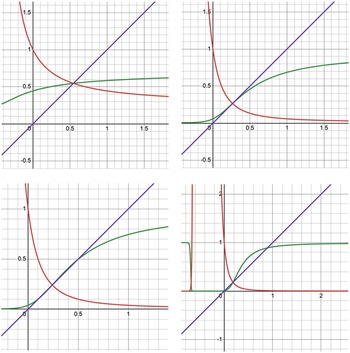
 f=f(1,x)
 f∘f
f∘f y=x
y=x d
d d=2
d=2 d=7
d=7 d=8
d=8 d=12
d=12 f∘f
f∘f d≥8
d≥8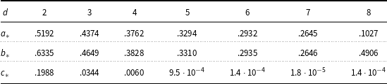
 φ
φ a=0,b=1,c=.9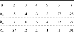
 a∗,b∗,c∗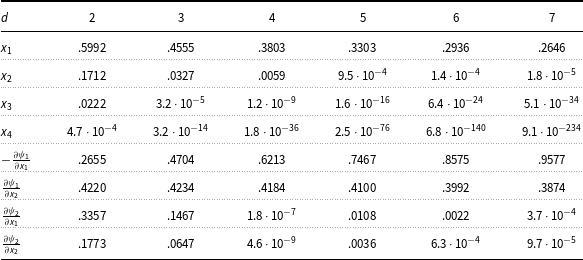
 x∗
x∗ ψ
ψ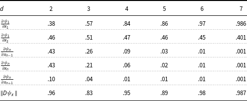
 x∈Sa,b,c
 (a,b,c)
 a,b,c
a,b,c n≥2
n≥2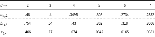
 cg,acg,bcg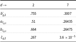
 c~g,ac~g,2,bc~g2
 d=2,7
d=2,7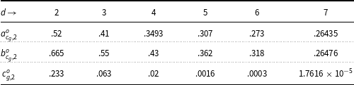
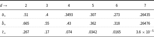

 Open access

