


Introduction
Between 2015 and 2018, three geothermal wells were drilled in Mol, northern Belgium (Bos & Laenen, Reference Bos and Laenen2017; Broothaers et al., Reference Broothaers, Bos, Lagrou, Harcouët-Menou and Laenen2019). The aim of the boreholes was twofold: (i) exploring the reservoir characteristics and geothermal potential of Lower Carboniferous carbonates and the underlying Devonian sandstones and (ii) developing a geothermal system for heat and power generation. The wells MOL-GT-01-S1, MOL-GT-02-S1 and MOL-GT-03-S1 (sidetracks will not be mentioned in the rest of the paper) reached depths of respectively 3610 m, 3830.2 m and 4238 m (true vertical depth (TVD)). MOL-GT-03 transected the entire Lower Carboniferous section and entered the Devonian. The first and third boreholes were drilled as production wells, aiming at a fault in the Lower Carboniferous reservoir. The second borehole is an injection well, deviated away from this interpreted fault.
Core material, cuttings and geophysical well logs of the three boreholes provide valuable information on the Lower Carboniferous carbonates in the Campine–Brabant Basin. The primary porosity of the limestones and dolostones is generally very low, in the order of a few per cent with exceptional peaks up to 10–20% (Vandenberghe et al., Reference Vandenberghe, Dusar, Boonen, Fan, Voets and Bouckaert2000; Piessens et al., Reference Piessens, Laenen, Nijs, Mathieu, Baele, Hendriks, Bertrand, Bierkens, Brandsma, Broothaers, de Visser, Dreesen, Hildenbrand, Lagrou, Vandeginste and Welkenhuysen2008; Reijmer et al., Reference Reijmer, Ten Veen, Jaarsma and Boots2017). Therefore, fractures are of major importance for reservoir permeability. The aim of this study is to assess the factors controlling the development and characteristics of fractures. Only 1.9 m of core material could be retrieved from a cored interval of 20.5 m in MOL-GT-01, which is not enough for a quantitative fracture study, and no coring was done in the other two boreholes. Therefore, fractures were identified by Schlumberger geologists from the Fullbore Formation MicroImager (FMI) log of the MOL-GT-01 borehole, based on resistivity contrasts. Since FMI and acoustic image logs result in an oriented image of the borehole wall, they provide valuable in situ information on the reservoir characteristics and are widely used to characterise geothermal reservoirs. Image logs have been studied to identify sedimentological and structural features in the subsurface, such as bedding planes, fractures and faults, and to obtain information on in situ stress orientations (Tenzer et al., Reference Tenzer, Mastin and Heinemann1991; Dezayes et al., Reference Dezayes, Villemin, Genter, Traineau and Angelier1995; Genter et al., Reference Genter, Castaing, Dezayes, Tenzer, Traineau and Villemin1997; Prensky, Reference Prensky, Lovell, Williamson and Harvey1999; Trice, Reference Trice, Lovell, Williamson and Harvey1999; Poppelreiter et al., Reference Poppelreiter, Garcia-Carballido, Kraaijveld, Pop- pelreiter, Garcia-Carballido and Kraaijveld2010; Massiot et al., Reference Massiot, McNamara and Lewis2015; Williams et al., Reference Williams, Toy, Massiot, McNamara and Wang2016; McNamara et al., Reference McNamara, Milicich, Massiot, Villamor, McLean, Sépulveda and Ries2019). Fractures and bed boundaries and their characteristics were quantified from the FMI log of the MOL-GT-01 borehole. Relationships of the fractures with bed thickness, lithology variations and the presence of faults were explored.
Geological setting
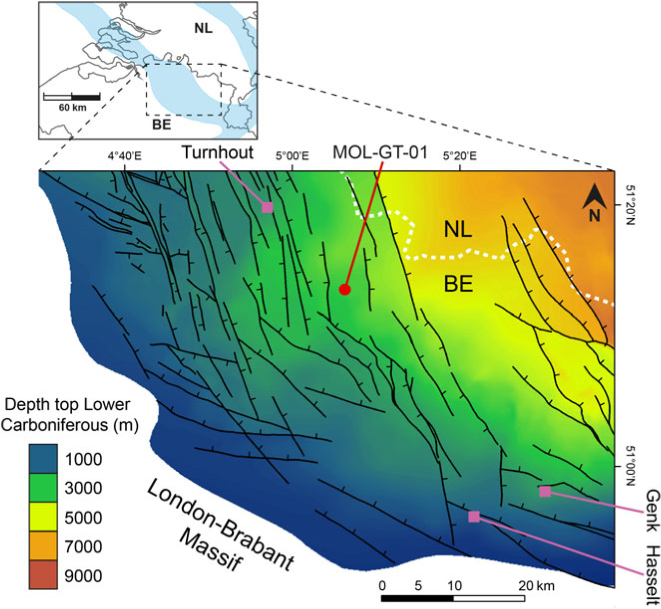
The three MOL-GT wells are located in the Campine–Brabant Basin (Fig. 1). During Early Carboniferous times, this Variscan foreland basin was present from the northern flank of the Caledonian London–Brabant Massif to the Zandvoort–Maasbommel–Krefeld High complex in the central Netherlands (Bless et al., Reference Bless, Bouckaert and Paproth1983). Lower Carboniferous ramp to shelf carbonates were deposited at the margins of the basin (Muchez et al., Reference Muchez, Viaene, Wolf and Bouckaert1987; Muchez, Reference Muchez1988; Muchez & Langenaeker, Reference Muchez and Langenaeker1993; Geluk et al., Reference Geluk, Dusar, de Vos, Wong, Batjes and de Jager2007; Kombrink et al., Reference Kombrink, Leever, Van Wees, Van Bergen, David and Wong2008).
Location of the MOL-GT-01 borehole in the Campine–Brabant Basin (modified after Van der Voet et al., Reference Van der Voet, Muchez, Laenen, Weltje, Lagrou and Swennen2020). The coloured map shows the depth of the top of the Lower Carboniferous, and the black lines indicate faults at this stratigraphic level (with a minimum throw of 30 ms on seismic), as interpreted by Deckers et al. (Reference Deckers, De Koninck, Bos, Broothaers, Dirix, Hambsch, Lagrou, Lanckacker, Matthijs, Rombaut, Van Baelen and Van Haren2019) based on 2D seismic data and borehole geophysical logs. The border between Belgium and the Netherlands is shown as a white dashed line.
The MOL-GT-01 borehole was drilled vertically. The top of the Lower Carboniferous carbonates was encountered at a depth of 3175.5 mMDBGL (metres measured depth below ground level) (Fig. 2; Van Gastel & Van Zutphen, Reference Van Gastel and Van Zutphen2016). The upper part of the Lower Carboniferous sequence is part of the Goeree Formation, down to 3227.5 m. This formation consists of an alternation of limestone and shale (and some minor intercalations described by mud loggers as marls), in which the amount of limestone decreases upwards and shale increases, towards the transition with the overlying Namurian shales (Souvré Formation). The rest of the drilled Lower Carboniferous sequence comprises the Loenhout Formation, from 3227.5 to 3610 m. This formation consists of limestone with minor intercalations of argillaceous limestone and shale. At a depth of 3507–3512.5 m, a dolostone level is present.
Bio-, chrono- and lithostratigraphy of the MOL-GT-01 borehole. The top of the Lower Carboniferous is located at 3175.5 m depth. The biostratigraphic analysis was done by Dr L. Hance. The chronostratigraphy was inferred from the biostratigraphic information using the correlation of Poty (Reference Poty2016). The lithological column is based on cuttings and geophysical well logs (Van Gastel & Van Zutphen, Reference Van Gastel and Van Zutphen2016). The depth of the cored intervals is also indicated.

In the Belgian part of the Campine–Brabant Basin, a pattern of mainly (N)NW–(S)SE-striking normal faults resulted in compartmentalisation of the Lower Carboniferous carbonates into fault blocks (Fig. 1; Bless et al., Reference Bless, Boonen, Dusar and Soille1981; Langenaeker, Reference Langenaeker2000; Laenen et al. Reference Laenen, Van Tongeren, Dreesen and Dusar2004; McCann, Reference McCann2008; Deckers et al., Reference Deckers, De Koninck, Bos, Broothaers, Dirix, Hambsch, Lagrou, Lanckacker, Matthijs, Rombaut, Van Baelen and Van Haren2019). Some of the normal faults were already active during the Devonian and/or early Carboniferous (Muchez & Langenaeker, Reference Muchez and Langenaeker1993; Reijmer et al., Reference Reijmer, Ten Veen, Jaarsma and Boots2017). Indications of pre-Cretaceous reverse fault movements were found near the Belgian mining area, c.30 km southeast of the MOL-GT-01 borehole (Deckers et al., Reference Deckers, De Koninck, Bos, Broothaers, Dirix, Hambsch, Lagrou, Lanckacker, Matthijs, Rombaut, Van Baelen and Van Haren2019). These faults are interpreted to be linked to late to post-Variscan wrench tectonics during Stephanian–Early Permian times (van Wees et al., Reference Van Wees, Stephenson, Ziegler, Bayer, McCann, Dadlez, Gaupp, Narkiewicz, Bitzer and Scheck2000; McCann, Reference McCann2008) and their throw decreases towards the northwest. The largest normal fault activity in northern Belgium took place during the Jurassic late Cimmerian phase. At these times, the London–Brabant Massif was uplifted and the Roer Valley Graben developed by fault-controlled subsidence in the Netherlands, northeastern Belgium and western Germany (Langenaeker, Reference Langenaeker2000; Deckers et al., Reference Deckers, De Koninck, Bos, Broothaers, Dirix, Hambsch, Lagrou, Lanckacker, Matthijs, Rombaut, Van Baelen and Van Haren2019). Deposits in the Belgian part of the Campine–Brabant Basin were tilted and many of the older faults were reactivated. The Roer Valley Graben was inverted during the late Cretaceous (Rossa, Reference Rossa1986; Langenaeker, Reference Langenaeker1999). Reverse fault movements were reconstructed based on seismic data and thickness variations, and inversion intensity decreases from the graben towards the southwest. Evidence for reverse fault movements is only found in the eastern part of the Belgian Campine area, c.25 km southeast of the MOL-GT-01 borehole (Deckers et al., Reference Deckers, De Koninck, Bos, Broothaers, Dirix, Hambsch, Lagrou, Lanckacker, Matthijs, Rombaut, Van Baelen and Van Haren2019). The inversion was succeeded by normal faulting during the Tertiary, which mostly compensates the previous reverse movements.
In the direct vicinity of the MOL-GT-01 borehole, normal faults are mostly NNW–SSE to almost N–S oriented (Deckers et al., Reference Deckers, De Koninck, Bos, Broothaers, Dirix, Hambsch, Lagrou, Lanckacker, Matthijs, Rombaut, Van Baelen and Van Haren2019). On the seismic line closest to the MOL-GT-01 borehole (c.350 m distance), normal faults are observed in the Upper Carboniferous section, but their continuation at deeper levels is uncertain due to lower quality of the seismic data (Broothaers et al., Reference Broothaers, Bos, Lagrou, Harcouët-Menou and Laenen2019).
Methodology
FMI log acquisition and processing
In the MOL-GT-01 borehole, a slim version of the FMI tool was used, which means that only pads without flaps were used, due to hole size restrictions and to avoid damaging the tool when opening the pads. This version of the tool contains 96 microelectrodes, and the borehole circumferential coverage is reduced by 50% compared to a tool with flaps. A standard FMI processing workflow was used, with a quality control of the accelerometer and magnetometer data to validate the orientation of the data. Speed correction was applied in the field to correct for any depth offset or irregular tool movements, and button harmonisation was performed to correct for the effects of different responses between buttons. Pad concatenation and orientation was done to create an oriented array in which each pad is in its correct position around the borehole. Finally, a dynamic and static normalisation of the corrected image data was done with a dynamic window of 2 ft (0.6096 m). A subsequent quality control of the final FMI images showed that only 3% of the data were of ‘moderate to poor quality’, due to sticking effects. These intervals were left out for further analyses.
Quantification of feature characteristics
Schlumberger geologists identified different features on the FMI log. Most of them are conductive features, which means they have a larger electrical conductivity than the rock matrix and appear as ‘dark’ features on the FMI log, i.e. conductive fractures, bed boundaries and stylolites. Resistive features appear lighter than the rock matrix. Only 18 resistive fractures were observed, which is much less than the number of conductive fractures. These resistive fractures are interpreted to be completely cemented by minerals and are not taken into account in this study since they do not contribute to permeability. Also, three borehole breakouts were identified, appearing as a pair of obscured stripes with an angle of 180° in between, which indicate a minimum horizontal stress of roughly WSW–ENE.
The aim of this study is to investigate the effect of bed thickness, lithology and faults on natural (partially) open fractures. These would appear on the FMI log as conductive sinusoids. However, they need to be distinguished from bed boundaries and drilling-induced tensile fractures, which are also observed as conductive features. The difference between bed boundaries and fractures is based on three observations. Firstly, bed boundaries are almost always full sinusoids, while fractures can be more frequently discontinuous. Secondly, fractures often cross-cut other features, while bedding planes do not. Finally, based on knowledge from seismic and cores and geophysical well logs of other boreholes, we know that bed boundaries are mostly gently dipping, while fractures mostly have higher angles. Because this study focuses on natural (partially) open fractures, these should also be distinguished from drilling-induced fractures. This difference is based on the fact that drilling-induced fractures show conductive discontinuities on opposite sides of the borehole, while natural fractures mostly appear as sinusoids. Trice (Reference Trice, Lovell, Williamson and Harvey1999) elaborates on the interpretation of features from image logs in more detail.
The interpreted features which were used in this study are defined as follows:
Bed boundaries: planar features which appear on the enrolled FMI log as (parts of) sinusoids. These are interpreted as depositional laminations which are bounding surfaces between individual beds, filled with more conductive material such as clays.
Conductive (natural) fractures: continuous or discontinuous mostly steeply dipping conductive planar features, often cross-cutting other features, appearing as (parts of) sinusoids. They are interpreted as natural fractures filled with material that is more conductive than the host rock, which could be for instance clay, mud or saline water. These features are referred to as ‘conductive fractures’ in this paper.
Drilling-induced tensile fractures: irregular features, appearing as lines on opposite sides of the borehole (180° difference). They were interpreted to be generated by the drilling of the borehole, and their strike is parallel to the in situ maximum horizontal stress, which is roughly NNW–SSE in this case (Fig. 3).
Fig. 3.Inclination (A) and azimuth (B) of drilling-induced fractures, interpreted from the FMI log. Drilling-induced features appear as two traces at opposite sides of the borehole (180° in between), as visible in the azimuth plot (B). Drilling-induced fractures form parallel to the maximum horizontal stress, which is approximately NNW–SSE in this case, slightly changing from c.N170E in the upper part to c.N150E in the lower part of the Lower Carboniferous section.


The features were manually picked on the FMI log by Schlumberger, using both the static and dynamic log for interpretation. By picking the features, the azimuth and dip were determined.
The chance of intersecting a vertical fracture with a vertical borehole is smaller than intersecting a horizontal fracture. To compensate for this sampling bias, the measured fracture frequency (number per metre) should be corrected prior to analyses. According to Terzaghi (Reference Terzaghi1965), a weighting factor was assigned to each fracture:
 $$w = {1 \over {\cos \alpha }}$$
in which w is the weighting factor and α is the angle between the fracture plane normal and the borehole, i.e. the fracture’s apparent dip. This weighting factor tends to infinity for fractures which are almost parallel to the borehole (almost vertical in this case). This is incorrect, since the chance of transecting a vertical fracture with a vertical borehole is not zero. Many different ways were proposed to correct for this problem. However, most of these methods contain assumptions that are not applicable in this study, such as the assumption that all fractures completely transect the borehole (Davy et al., Reference Davy, Darcel, Bour, Munier and de Dreuzy2006) or that all fracture planes are ellipse-shaped (Mauldon & Mauldon, Reference Mauldon and Mauldon1997). Furthermore, methods such as Mauldon & Mauldon’s (Reference Mauldon and Mauldon1997) would result in the most realistic values, but require information that is not available in this study, such as the length of the two axes of a fracture ellipse. Alternatively, an arbitrary cut-off angle of 10° between the fracture and the borehole is often used to prevent overestimation of sub-vertical fractures (Yow, Reference Yow1987). In this study, a maximum weighting factor of 1/cos(80°) was applied. Figure 4A shows the measured frequency of conductive fractures along depth, Figure 4B the inclination of these fractures and Figure 4C the Terzaghi-corrected fracture frequency along depth. These corrected fracture frequencies are used to analyse the relationship between lithology and fracture frequency and between fault presence and fracture frequency.
Measured frequency (A) and inclination (B) of conductive fractures are plotted along borehole depth. In (C), the fracture frequency of (A) is corrected for sampling bias based on fracture inclination. The green line shows the depth of the fault intersection with the highest confidence. The blue and purple lines represent the fault intersections with a lower confidence level.

Fault interpretations
The quantified inclination and azimuth of bed boundaries enabled identification of zones in which sudden changes in bedding characteristics are present. We used a dip change of minimum 25° or an azimuth change of at least 90°. These changes were determined by analysing diplogs and walkout azimuth plots. A bedding inclination that rapidly increases and decreases again with depth, also referred to as a ‘cusp’ (Bengtson, Reference Bengtson1981; Fossen, Reference Fossen2010), is often used for fault identification (Etchecopar & Bonnetain, Reference Etchecopar and Bonnetain1992; Hurley, Reference Hurley1994; Schlumberger, 1997; Hesthammer & Fossen, Reference Hesthammer and Fossen1998; Lai et al., Reference Lai, Wang, Wang, Cao, Li, Pang, Han, Fan, Yang, He and Qin2018). Such a cusp was originally interpreted as the result of ‘fault drag’, thought to be caused by frictional sliding along a fault. However, Ferrill et al. (Reference Ferrill, Morris and McGinnis2012) proposed that a cusp associated with normal faults in mechanically layered rocks results from ‘fault-tip folding’ prior to propagation of the fault. In other words, if a fault tip enters a mechanically weak layer during continuous fault slip, the fault cannot propagate but instead ductile deformation (folding) occurs to accommodate the displacement gradient. In such a case, a monocline forms beyond the fault tip (Gawthorpe et al., Reference Gawthorpe, Sharp, Underhill and Gupta1997; Janecke et al., Reference Janecke, Vandenburg and Blankenau1998; Hardy & McClay, Reference Hardy and McClay1999; White & Crider, Reference White and Crider2006; Ferrill & Morris, Reference Ferrill and Morris2008). This process is also referred to as ‘forced folding’ (Withjack et al., Reference Withjack, Olson and Peterson1990; Schlische, Reference Schlische1995; Tavani et al., Reference Tavani, Balsamo and Granado2018). Such a monocline above a fault tip has also been observed in outcrop (Ferrill & Morris, Reference Ferrill and Morris2008). After this kind of folding, the fault can still propagate through the folded layers. The presence of a cusp on itself does not provide information about the fault type, i.e. a normal fault or reverse fault.
A sudden change in azimuth could be caused by a fault as well, but also by an unconformity or a fold. From the relationship between the sudden change in azimuth and the evolution of the inclination with depth in its vicinity, it is possible to better define which one of the above causes the azimuth change. Using both the inclination and azimuth changes, all possible fault intersections were described.
Data analysis and statistical testing
Non-parametrical Kruskal–Wallis and Wilcoxon tests were performed on the transformed variables for studying the relationships with categorical variables, such as lithology and interpreted fault zones (Davis, Reference Davis2002). A Principal Component Analysis (PCA) was performed on the lithology-dependent geophysical well logs combined with the fracture variables, in order to visualise the relationships between these variables.
Variable transformations are necessary prior to analyses, to eliminate the restrictions of their original values. A log transformation is performed on all variables of which the values cannot be negative. Zero-values were replaced by a chosen constant (for instance 0.1) by adding this constant to all values before log transformation. The inclination variables contain values restricted by 0° and 90° and therefore require the following transformation:
 $$T(x) = \log \left({{{x_i} + c} \over {b - {x_i} + c}}\right)$$
in which xi is the original variable, b is the positive restriction value, c is a chosen constant to eliminate 0-values and T is the transformed variable.
Results
Quantified features
Apparent bed thicknesses were calculated as the distance between two sequential bed boundaries. These values were corrected for the borehole inclination (maximum 4.06°) to calculate the vertical bed thickness. Finally, this vertical bed thickness was multiplied by the sinus of the bed’s inclination (average of the overlying and underlying bed boundary), to arrive at the true bed thickness. These true bed thicknesses are plotted along the depth of the borehole in Figure 5. The thickest bed is 57 cm and the mean thickness is 2 cm. Beds are clearly thickest in the zone between 3225 and 3310 m depth. At the base of the sequence (3450–3604 m) and in the top zone (3175.5–3225 m), beds are relatively thin. In the intervals from 3276 to 3277 m and 3279 to 3284 m, the FMI signal was affected by acquisition or borehole artefacts in such a way that no interpretations could be made. Therefore, no bed thickness could be calculated for this section.
True bed thickness along the depth of the MOL-GT-01 borehole. These bed thicknesses are calculated from the apparent bed thickness, which was corrected for the borehole inclination and the inclination of the bed itself.

Bed thickness and fracture frequency
In order to correctly analyse the relationship between bed thickness and fracture frequency, the interval from 3330 to 3510 m was used. In this part of the section, the FMI log shows no indication for the presence of faults (see ‘Faults’ subsection below). Beds with a true thickness of less than 0.5 cm were not taken into account for the further analyses. Based on the depths of the fracture midpoints and the depths of the bed boundary midpoints, the number of fracture intersections per bed was calculated. The chance of intersecting a fracture in a steeply dipping bed is larger than in a horizontal bed, because most fractures are approximately perpendicular to bedding. Therefore, the number of fractures per bed was corrected by multiplying it with a weighting factor based on the inclination of the bedding:
 $$w = {1 \over {\sin \alpha }}$$
in which w is the weighting factor and α is the inclination of the bed (average of over- and underlying bed boundary). Similar to the Terzaghi correction applied on the fracture frequency, as mentioned before, a cut-off value should be used in order not to overestimate the fractures in horizontal beds. In this case, a maximum weighting factor of 1/sin(10°) was applied.
The resulting corrected number of fracture intersections per bed was subdivided into categories: beds with 0 fracture intersections, beds with 1 to 6 fracture intersections, etc. All beds with 12 or more fracture intersections were combined in one category. Figure 6A shows these categories plotted against the true bed thickness (logarithmic scale). On average, more fractures are present in thick beds than in thin beds. This is not surprising, as the chance to be intersected by a fracture is higher for a thick bed than for a thin one. However, this would be the case if the total number of fractures were spread out evenly along the entire section, so with a constant spacing. Of course, this is not the case in this borehole.
Results of the analysis investigating the relationship between bed thickness and fracture frequency. The true bed thickness variation (y-axis) is shown for the different categories of the number of fracture intersections per bed (x-axis). The results of the MOL-GT-01 borehole are plotted in (A). It is not surprising that thicker beds generally contain more fractures, but we also investigated the hypothetical case in which the same total number of fractures would be spread out evenly over the entire Lower Carboniferous interval, so with a constant spacing (B). In both plots, the fracture numbers are corrected using a weighting factor that depends on the bed inclination. The difference between the two situations is highlighted in Figure 4A, in red for the relatively thick beds and in blue for the relatively thin beds. Figure 4A shows that the thicker beds in the borehole contain relatively few fractures, and thinner beds relatively many. In both plots, only the beds between 3330 and 3510 m were taken into account, in order to exclude the possible influence of faults.

In order to determine the effect of bed thickness on fracture frequency, the real data from MOL-GT-01 should be compared to this hypothetical situation. The results of the hypothetical situation are shown in Figure 6B. This is calculated by subdividing the total number of fractures in the entire section (found in the real situation) by the length of the total section, to obtain the theoretical constant vertical spacing between the fractures. With this spacing, the depths of the theoretical fractures were calculated. Based on these depths and the depths of the real bed boundaries, the theoretical number of fracture intersections per bed was determined. These fracture numbers should be corrected for the bedding inclination, similar to the method used for the fracture numbers of the real data. These corrected theoretical fracture numbers are also subdivided into categories, as plotted on the x-axis of Figure 6B.
The bed thickness of each category shows a clearly larger variation in the real situation than in the hypothetical situation. The differences are marked in red (thicker beds) and blue (thinner beds) in Figure 6A. In the hypothetical case, the thickest beds (>0.18 m) contain more than 6 fractures (corrected by weighting factor). The data from MOL-GT-01, however, also show low fracture numbers (1–6 and even 0) for these same thick beds. The hypothetical case shows that thin beds (<0.01 m) contain no more than 6 fractures, while the data from MOL-GT-01 show that these thin beds can contain up to 12 fractures or more. So, thin beds contain relatively many fractures and thick beds relatively few fractures in the case of the MOL-GT-01 borehole. Also when taking into account the entire Lower Carboniferous section, including the possible fault zones, the result is similar. The analysis was also performed on the different lithologies separately. A large majority of the sequence consists of limestone, in which relatively thick beds contain relatively few fractures. In dolostone intervals, the same effect is visible but less clear. In shaly intervals and argillaceous limestone intervals, no such effect is visible. In these lithologies, the fracture distribution is very similar to the situation in which fracture spacing would be constant.
Lithology
Lithology variations
The geophysical well logs which mostly reflect lithological characteristics are the density log, the spectral gamma-ray log and the photoelectric absorption (PEF) log. In Figure 7, these three logs are plotted next to the lithology that was derived from the cuttings and log data (Fig. 2). A cluster analysis with a Euclidean distance measure was performed on the transformed variables of the three geophysical well logs combined, in order to check whether there are significant clusters, or whether all data points belong to the same statistical population. In this way, seven significant clusters were identified, based on the three lithology-dependent logs. The colours of the data points in Figure 7 indicate the different clusters. These cluster results roughly coincide with the variations in the litholog. Moreover, the fact that there are different clusters means that there are significant lithology variations which need to be taken into account in the further analyses.
Spectral gamma-ray log, density log and photoelectric absorption (PEF) log along the lithological column of the MOL-GT-01 Lower Carboniferous interval. The colours of the geophysical-well-log data points represent the result of a cluster analysis based on the three geophysical logs combined. The dashed lined boxes indicate the faulted zone (upper box; F) and the non-faulted zone with a similar lithology (lower box; NF) which were compared to analyse the effect of faults on the fracture frequency.

Lithology and fractures
Figure 8 shows the results of a PCA of the lithology-dependent geophysical well logs with the Terzaghi-corrected frequency of the conductive fractures. The density and PEF log variables are positioned almost perpendicular to the fracture frequency, which means that these two log variables are almost uncorrelated to fracture frequency. The spectral gamma-ray log variable is oriented almost in the opposite direction to the fracture frequency. This indicates a negative correlation between the gamma-ray log and the fracture frequency. The PCA suggests that the impact of lithology on the fracture characteristics is limited: shaly beds seem to have lower fracture frequencies than the carbonate beds. The absence of a correlation with the density log and PEF log indicates that there is no or limited impact of the dolomite or quartz content on the fracture characteristics of the carbonate beds.
Results of a Principal Component Analysis (PCA) of different transformed variables, which was performed to analyse relationships between the variables. The variables taken into account are: the spectral gamma-ray log, density log, PEF log and the corrected conductive fracture frequency. The figure shows that the fracture frequency is almost uncorrelated to the density and PEF logs (arrows almost perpendicular), while it is negatively correlated to the spectral gamma-ray log (arrows almost parallel in opposite direction). The first and second principal components together explain 62.5% of the data variability.

In order to analyse whether or not the fracture frequency differs between the lithologies derived from cutting and logs, the section was subdivided into intervals of 0.5 m. Each interval was assigned one of the five lithology categories shown in the litholog (Fig. 2), i.e. shale, argillaceous limestone, limestone, dolostone or marl. A Kruskal–Wallis test was run to check whether there are significant differences in fracture frequency between the lithology categories. The result shows that shales contain lower conductive fracture frequencies than limestone and dolostone, but no significant differences were found between the latter two. This result is in line with the outcomes of the PCA shown in Figure 8.
Faults
Fault interpretations
Cusps and azimuth changes in the borehole were identified based on the FMI results. At least one very clear cusp was observed at 3284 m depth (Fig. 9). Between 3278 and 3295 m, the azimuth of the bed boundaries hardly changes, showing a NNW–SSE strike and dip towards the west-southwest. However, the dip increases in this section from 3273 to 3279 m and decreases again from 3284 to 3295 m. This is a clear example of a cusp, which could be interpreted as the result of a WSW-ward dipping normal fault or an ENE-ward dipping reverse fault, both with normal drag (Fig. 9). Based on the local and regional geological setting, the presence of a normal fault at this location is much more likely than a reverse fault. In case of a normal fault, the steeper bedding most likely results from fault-tip folding (Bengtson, Reference Bengtson1981; Fossen, Reference Fossen2010). Based on the available data, it is unclear whether a fault propagated into this section, or whether only fault-tip folding occurred without displacement.
Inclination and azimuth of bed boundaries interpreted from the FMI data of the 3270 to 3295 m interval (left). In the intervals indicated in grey, the FMI signal was affected by acquisition or borehole artefacts in such a way that no interpretations could be made. Bed boundaries are plotted as two stick-diagram cross-sections (right). A WSW-dipping normal fault or an ENE-dipping reverse fault, both with normal drag, could be interpreted. Also the possible faults at 3262 m and 3300 m are illustrated.

Another alternative explanation of the cusp is reverse (concave) drag of an ENE-ward dipping normal fault. However, reverse drag is less common than normal drag and would be expected resulting from a growth fault or listric fault, in which usually only the hanging wall shows drag as ‘rollover in the downthrown block’ (Schlumberger, 1997; Fossen, Reference Fossen2010). In this borehole, bedding gradually steepens towards the fault at both sides of the fault.
The steepest bed boundary in this zone, which is located at 3283.94 m (just below the zone without interpretable FMI data), has an inclination of 54°. In the most probable case of a normal fault, the fault most likely has an inclination of at least 54°, since fault-tip folding causes the structural dip to be steepest at the fault plane or monocline centre (Ferrill et al., Reference Ferrill, Morris and McGinnis2012).
Other dip and azimuth variations along the borehole were also analysed (Fig. 10; Table 1). The total of eight inferred anomalies could possibly also be the result of faults, although the data are less conclusive than for the succession around 3284 m. These anomalies could resemble faults with a smaller throw and/or less folding. A relative confidence level was assigned to each of the anomalies, with 1 being the highest confidence that it is a fault intersection and 5 reflecting the lowest confidence. This is based on the amount of dip change, the amount of azimuth change, and other possible fault indications such as a higher rate of penetration (ROP), a lower weight on bit (WOB), a caliper anomaly or mud losses. The visibility of bed boundaries was also taken into account. For most of the possible faults, no (clear) fault plane is visible on the FMI log. However, the cusp at 3532 m depth is one of the few where a possible fault plane could be identified. Two conductive planar features were observed, which truncate stylolites or bed boundaries (Fig. 11), while the bedding dip and azimuth change only very slightly. The truncation could be the result of a fault, but could also reflect, for instance, a current incision or another sedimentary structure.
Bedding inclination (A) and azimuth (B) plotted along the depth of the borehole. Based on dip and azimuth changes of the bedding, eight possible fault intersections were identified. Taking into account the magnitude of the changes in dip and azimuth, as well as the visibility of bed boundaries and other fault indications such as drilling parameters, each possible fault was assigned a relative confidence level (1 being most confident). Only the four possible faults with a confidence level of 1 to 3 were taken into account for further analyses. See Table 1 for descriptions of each possible fault.

Characteristics of identified anomalies in structural dip (cusps) and azimuth, interpreted as possible faults

Two conductive planar features (blue) truncating two bedding planes or stylolites (green), visible on the FMI log of MOL-GT-01 at 3531.8 m depth. The features in blue were interpreted as a possible fault with a relative confidence level of 4 (Fig. 10).

Fault identification was needed to investigate whether fracture frequency is increased around these fault intersections. For these analyses, we only took into account the four identified faults with a relative confidence level of 1 to 3, because the uncertainty of the other possible fault intersections is rather large and in the case that these are indeed also faults, they most likely correspond to small discontinuities.
Faults and fracture characteristics
In order to analyse the effect of possible faults on fracture frequency, the fracture frequencies of the ‘faulted’ intervals were compared to an undisturbed interval with similar lithology. The zones around the four possible fault intersections (all between 3244 and 3300 m depth) were compared to the section between 3370 and 3450 m, which contains similar lithologies (Fig. 7). The zone with non-interpretable FMI records around the 3284 m cusp was not taken into consideration in this analysis. First, the mean corrected fracture frequency is calculated for all metre intervals within 1 m vertical distance of the four interpreted faults. The same is done for ‘fault zones’ of 2 m each side, 3 m, etc. These results are shown in Figure 12A. The largest tested fault zones are 70 m each side of the faults, because the distance between the deepest fault and the non-faulted zone with similar lithology is 70 m (Fig. 7). As seen in Figure 12A, fracture frequencies are higher close to the faults. ‘Fault zones’ up to c.45 m each side of the fault show higher mean fracture frequencies than the non-faulted zone. A non-parametrical Wilcoxon test was then performed to test whether the fracture frequency difference between the fault zone metre-intervals and the non-faulted zone metre-intervals is significant. This was repeated for fault zones of different sizes, from 1 to 70 m again. The resulting p-values of these tests are shown in Figure 12B. When using a confidence level of 95%, the difference is only significant if the p-value is lower than 0.05. Only when considering a ‘fault zone’ of 9 m each side, the fracture frequency within the fault zone is significantly higher than in the non-faulted zone with similar lithology. For smaller or larger fault zones, the fracture frequency is not significantly higher than this ‘background frequency’.
Results of the analysis investigating the relationship between the presence of faults and fracture frequency. (A) Mean corrected frequency of conductive fractures within zones around the four clearest faults (y-axis), for zones with different vertical sizes (x-axis). The dashed line indicates the mean corrected conductive fracture frequency in a non-faulted zone with a similar lithology. The results show that mean fracture frequencies are increased in the vicinity of faults. The difference in (corrected and log-transformed) fracture frequency between the fault zones and the non-faulted zone was tested using a Wilcoxon test. (B) The resulting p-values of these tests for the different fault zone sizes. When using a confidence level of 95%, the difference is significant if the p-value is lower than 0.05, which is only the case for fault zones of 9 m each side. For all other fault zone sizes, the fracture frequency is not significantly higher than the ‘background frequency’.

Apart from the frequency, the inclination of fractures is also different in the vicinity of faults (Fig. 4). Fractures are more horizontal (lower inclination) closer to faults than away from faults.
Interpretation and discussion
Bed thickness and fractures
The analyses show that thick beds contain relatively few fractures, and thin beds relatively many. This result is in line with various studies that found that fracture spacing is proportional to bed thickness (Bogdonov, Reference Bogdonov1947; Price, Reference Price1966; Hobbs; Reference Hobbs1967; Sowers, Reference Sowers1972; Narr & Suppe, Reference Narr and Suppe1991; Gross, Reference Gross1993). Bai et al. (Reference Bai, Pollard and Gao2000) proposed an explanation for this relationship. Experimental studies showed that fracture spacing first decreases with increasing extensional strain perpendicular to the fractures. At a certain ratio between spacing and bed thickness, no new fractures form and instead, opening of the existing fractures increases to accommodate the increasing strain. This is called ‘fracture saturation’ and this causes the relationship between bed thickness and fracture spacing/frequency. Experiments of Bai et al. (Reference Bai, Pollard and Gao2000) showed that this fracture saturation could be caused by the normal stress between fractures that changes from tensile to compressive, with increasing applied stress.
In the case of MOL-GT-01, there is no such clear correlation between bed thickness and fracture frequency, since variation is large. However, a similar trend is present with thinner beds containing more fractures, as reported widely in the literature.
Lithology and fractures
The relationship between fracture frequency and lithology seems limited, based on PCA results. Only the spectral gamma-ray log shows a negative correlation to fracture variables, which means that intervals with higher spectral gamma-ray signal contain slightly fewer fractures. This is supported by the results of the Kruskal–Wallis tests, which show that shaly intervals contain fewer conductive fractures than limestone and dolostone. Studies on rock strength have shown that shales are less competent than limestones and dolostones (Donath, Reference Donath1970; Ferrill & Morris, Reference Ferrill and Morris2008; Alzayer, Reference Alzayer2018). This means that shales can accommodate more pre-failure strain than limestones and dolostones. Therefore, limestone and dolostone fracture earlier under the same stress conditions. So, it is not surprising that lower fracture frequencies were found in shaly layers than in limestone and dolostone.
Geometry of possible faults
The possible fault at 3284 m depth was identified because of its clear diplog cusp-pattern. This cusp could be the result of a normal fault or a reverse fault. If it is a reverse fault with normal drag, it is dipping towards ENE. However, based on the local and regional geological setting, it most likely corresponds to a normal fault with fault-tip folding. For such ductile deformation to occur, mechanically weak layers must be present (Ferrill & Morris, Reference Ferrill and Morris2008; Ferrill et al., Reference Ferrill, Morris and McGinnis2012). Shale layers can generally accommodate more pre-failure strain than limestone or dolostone. A number of shale layers and argillaceous limestone beds are present in the stratigraphy of the Lower Carboniferous in MOL-GT-01, which possibly accommodated such fault-tip folding. This does not necessarily imply that fault displacement occurred.
No obvious thickness variations or missing units were found when comparing the lithology-dependent geophysical well logs of the three boreholes to each other (Broothaers et al., Reference Broothaers, Bos, Lagrou, Harcouët-Menou and Laenen2019). This could mean that the dip-slip fault displacement is too small to be observed in the log correlation. A strike-slip displacement could be present either way, since it would not result in a missing stratigraphic section. In case of a normal fault, it is also possible that no fault displacement has occurred at this location and depth and that the dip anomaly results purely from ‘fault-tip folding’, or ‘forced folding’ (Fig. 13, phase 2).
Schematic model showing the process of fault-tip folding and subsequent fault propagation. Phase 1 represents the original situation with gently dipping carbonates with some fractures. Phase 2 is the fault-tip folding as a result of a normal fault in underlying strata. At this stage, fractures develop as a result of folding. In phase 3, the fault propagates into the folded strata. If the cusps in MOL-GT-01 represent fault-tip folding of a normal fault, the observed cusps could represent either the situation of phase 2 or phase 3. Vertical scale would be a few tens of metres in phase 2 and 3.

In the case that normal fault displacement did occur, the inferred orientation of this possible fault coincides with the general orientation of normal faults in the area around MOL-GT-01. The ‘fault’ is interpreted to be dipping towards WSW and striking NNW–SSE. This orientation matches with the larger-scale faults interpreted from seismic data by Deckers et al. (Reference Deckers, De Koninck, Bos, Broothaers, Dirix, Hambsch, Lagrou, Lanckacker, Matthijs, Rombaut, Van Baelen and Van Haren2019). Because the borehole breakouts and drilling-induced fractures indicate that the in situ maximum horizontal stress is oriented NNW–SSE, this WSW-dipping normal fault would be dip-slip.
Fracture frequency near possible faults
The frequency of conductive fractures is, on average, larger within zones that are no more than 45 m from the interpreted possible fault intersections (vertically each side) than outside these zones. However, since the differences between ‘fault zone frequency’ and ‘background frequency’ are mostly not significant, no clear ‘damage zones’ are present in this borehole (Faulkner et al., Reference Faulkner, Jackson, Lunn, Schlische, Shipton, Wibberley and Withjack2010; Peacock et al., Reference Peacock, Dimmen, Rotevatn and Sanderson2017). Johri et al. (Reference Johri, Zoback and Hennings2014) did interpret damage zones around faults from image logs; they encountered damage zones of 50 to 80 m in total. McNamara et al. (Reference McNamara, Milicich, Massiot, Villamor, McLean, Sépulveda and Ries2019) found high fracture density zones both within and outside projected fault zones in four boreholes, in volcanic lithologies. A spatial correlation between fault zones and larger fracture densities was only found in one of the boreholes. Williams et al. (Reference Williams, Toy, Massiot, McNamara and Wang2016) found that fracture density did not increase with proximity to the principal slip zones of faults (max. 30 m away from the slip zone). They found a stronger lithological influence instead. Cores have also been studied to assess the relationship between faults and fracture densities. Choi et al. (Reference Choi, Edwards, Ko and Kim2016) studied fractured fault zones from two borehole cores and found damage zones ranging from several metres to about 100 m, by analysing a cumulative distribution of fractures.
The smaller inclination of fractures within ‘fault zones’ could be the result of fault-tip folding. In folds, longitudinal fractures develop parallel to the axis of the fold and roughly perpendicular to the bedding, as a result of outer arc extension (Fischer & Wilkerson, Reference Fischer and Wilkerson2000). A steeper bedding close to a fault plane or monocline centre therefore leads to fractures with a smaller inclination (Fig. 13). Such a rotation of fractures in a normal fault zone was documented in an outcrop by Kim et al. (Reference Kim, Peacock and Sanderson2004).
Conclusions
Factors controlling the development and characteristics of fractures were evaluated using the FMI log and lithology of the Lower Carboniferous section of well MOL-GT-01. The analyses led to the following conclusions:
In well MOL-GT-01, thick beds contain relatively few conductive fractures and thin beds relatively many.
The conductive fracture frequency is only slightly dependent on lithology. The only significant differences are the lower fracture frequency in shaly intervals compared to limestone and dolostone. The dolomite and quartz content in carbonates do not have a significant impact on the fracture properties.
Eight zones with sudden changes in the dip and/or azimuth of bed boundaries were identified. The clearest cusp is present at a depth of 3284 m. This cusp could be caused by a WSW-ward-dipping normal fault, or an ENE-ward-dipping reverse fault. Based on the local and regional geology, the presence of a normal fault is most likely. In this case, the dip anomaly likely results from associated fault-tip folding (also known as forced folding). It is uncertain whether fault displacement took place or whether the borehole transected an overlying monocline.
Based on the four clearest faults, the mean conductive fracture frequency is increased in the vicinity of faults. Up to a vertical distance of c.45 m from the faults, mean fracture frequencies are larger compared to a non-faulted interval with similar lithology. However, these differences are mostly not significant, so no clear damage zones are present.
Acknowledgements
The presented work was supported by a VITO PhD grant, nr. 1610424. A biostratigraphic analysis was performed by Dr Luc Hance, for which we are very grateful. We would like to thank Stijn Bos (VITO), Jef Deckers (VITO) and Prof. Manuel Sintubin (KU Leuven) for valuable and constructive discussions which helped to improve the manuscript. We very much appreciate the constructive and detailed feedback of Dr David McNamara and an anonymous reviewer. We also appreciate the work of associate editor Hans Veldkamp.


 Open access

