

1 INTRODUCTION
Astrophysical magnetic fields are often modelled using ideal magnetohydrodynamics (MHD), which assumes that the gas is fully ionised and that the electrons are tied to the magnetic field and have zero resistivity. However, in molecular cloud cores, for example, this has been known to be a poor approximation to the true conditions since at least Mestel & Spitzer (Reference Mestel and Spitzer1956), where the ionisation levels can be as low as
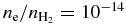 $n_{\text{e}}/ n_{\text{H}_{2}} = 10^{-14}$
(Nakano & Umebayashi Reference Nakano and Umebayashi1986; Umebayashi & Nakano Reference Umebayashi and Nakano1990).
$n_{\text{e}}/ n_{\text{H}_{2}} = 10^{-14}$
(Nakano & Umebayashi Reference Nakano and Umebayashi1986; Umebayashi & Nakano Reference Umebayashi and Nakano1990).
When a medium is only partially ionised, such as in a molecular cloud, three non-ideal MHD effects occur:
-
1. Ohmic resistivity: the drift between electrons and ions/neutrals; neither ions nor electrons are tied to the magnetic field,
-
2. Hall effect: ion-electron drift; only electrons are tied to the magnetic field, and
-
3. Ambipolar diffusion: ion-neutral drift; both ions and electrons are tied to the magnetic field.
These environmentally dependent terms add resistivity to the electrons, and ultimately affect the evolution of the magnetic fiels (e.g. Wardle & Ng Reference Wardle and Ng1999; Nakano, Nishi, & Umebayashi Reference Nakano, Nishi and Umebayashi2002; Tassis & Mouschovias Reference Tassis and Mouschovias2007; Wardle Reference Wardle2007; Pandey & Wardle Reference Pandey and Wardle2008; Keith & Wardle Reference Keith and Wardle2014). Recent studies, both idealised (e.g. Bai Reference Bai2014, Reference Bai2015) and realistic (e.g. Shu et al. Reference Shu, Galli, Lizano and Cai2006; Mellon & Li Reference Mellon and Li2009; Duffin & Pudritz Reference Duffin and Pudritz2009; Dapp & Basu Reference Dapp and Basu2010; Krasnopolsky, Li, & Shang Reference Krasnopolsky, Li and Shang2010; Machida, Inutsuka, & Matsumoto Reference Machida, Inutsuka and Matsumoto2011; Li, Krasnopolsky, & Shang Reference Li, Krasnopolsky and Shang2011; Dapp, Basu, & Kunz Reference Dapp, Basu and Kunz2012; Tomida et al. Reference Tomida, Tomisaka, Matsumoto, Hori, Okuzumi, Machida and Saigo2013; Tomida, Okuzumi, & Machida Reference Tomida, Okuzumi and Machida2015; Tsukamoto et al. Reference Tsukamoto, Iwasaki, Okuzumi, Machida and Inutsuka2015a, Reference Tsukamoto, Iwasaki, Okuzumi, Machida and Inutsuka2015b; Wurster, Price, & Bate Reference Wurster, Price and Bate2016) have included some or all of the non-ideal MHD effects. In each study, however, the authors have been required to write and implement their own algorithms to model the non-ideal MHD effects.
Multiple algorithms existing within a community provides a self-consistent check on the processes, and this helps to validate the results. However, writing and implementing the non-ideal MHD algorithms is a non-trivial process, both physically and numerically. Thus, we introduce Nicil: Non-Ideal MHD Coefficients and Ionisation Library, which is a pre-written, Fortran90 module that self-consistently calculates the non-ideal MHD coefficients and is ready for download and implementation into existing codes. Early version of Nicil are used in Wurster et al. (Reference Wurster, Price and Bate2016) and Wurster, Price, & Bate (in preparation). We are aware that a similar stand-alone code has recently been published by Marchand et al. (Reference Marchand, Masson, Chabrier, Hennebelle, Commerçon and Vaytet2016).
This paper is a user-manual for Nicil, and is organised as follows. Section 2 describes the algorithms that Nicil uses. We perform a simple test of Nicil in Section 3, and provide an astrophysical example in Section 4. Section 5 explains how to implement Nicil into an existing numerical code, and we conclude in Section 6. Throughout the text, we will refer to the ‘author’ as the author of Nicil, the ‘user’ as the person who is implementing Nicil into the existing code, and the ‘user’s code’ or ‘existing code’ as the code into which Nicil is being implemented.
2 ALGORITHMS
The complete Nicil library can be downloaded at www.bitbucket.org/jameswurster/nicil. This is a free library under the GNU license agreement: free to use, modify, and share, does not come with a warranty, and this paper must be cited if Nicil or any modified version thereof is used in a study. The important files are listed and summarised in Appendix A. The important parameters which the user can modify, along with their default values, are listed in Appendix B.
Nicil includes various processes that can be included or excluded at the user’s discretion. Major processes are cosmic ray and thermal ionisation (one or both can be selected) and the assumption of the grain size distribution (fixed or MRN distribution; Mathis, Rumpl, & Nordsieck Reference Mathis, Rumpl and Nordsieck1977). By default, all three non-ideal MHD coefficients are self-consistently calculated, however, Nicil includes the option of calculating only selected terms or using fixed coefficients (see Appendix C for a discussion of fixed coefficients).
The remainder of this section describes the processes that are used to calculate the non-ideal MHD coefficients. We define all variables, but for clarity, we do not state the default values in the main text.
2.1. Cosmic ray ionisation
When a cosmic ray (or an X-ray) strikes an atom or molecule, it has the ability to remove an electron which creates an ion. Two ion species are modelled: species i with mass
 $m_{\text{i}_{\text{R}}}$
, which represents the light elements (e.g. hydrogen and helium compounds), and species I with mass
$m_{\text{i}_{\text{R}}}$
, which represents the light elements (e.g. hydrogen and helium compounds), and species I with mass
 $m_{\text{I}_{\text{R}}}$
, which represents the metals. The light ion mass is calculated from the given abundances or mass fractions of hydrogen and helium assuming all the hydrogen is molecular hydrogen, and the metals are modelled as a single species, where the mass is a free parameter.
$m_{\text{I}_{\text{R}}}$
, which represents the metals. The light ion mass is calculated from the given abundances or mass fractions of hydrogen and helium assuming all the hydrogen is molecular hydrogen, and the metals are modelled as a single species, where the mass is a free parameter.
Dust grains have the ability to absorb electrons, which gives the grains a negative charge or lose an electron to give them a positive charge. Nicil includes two dust models: fixed radius and MRN size distribution. For a fixed grain size,
 $a_{\text{g}}$
, the number density is proportional to the total number density, n (Keith & Wardle Reference Keith and Wardle2014),
$a_{\text{g}}$
, the number density is proportional to the total number density, n (Keith & Wardle Reference Keith and Wardle2014),
 $$\begin{equation}
n_{\text{g}} = \frac{m_{\text{n}}}{m_{\text{g}}}f_{\text{dg}} n,
\end{equation}$$
$$\begin{equation}
n_{\text{g}} = \frac{m_{\text{n}}}{m_{\text{g}}}f_{\text{dg}} n,
\end{equation}$$
where
 $f_{\text{dg}}$
is the dust-to-gas mass ratio and
$f_{\text{dg}}$
is the dust-to-gas mass ratio and
 $m_{\text{n}}$
is the mass of a neutral particle.
$m_{\text{n}}$
is the mass of a neutral particle.
The number density for the MRN grain distribution follows a power law, viz.,
 $$\begin{equation}
\frac{\text{d}n_{\text{g}}}{\text{d}a} = An_{\text{H}}a^{-3.5},
\end{equation}$$
$$\begin{equation}
\frac{\text{d}n_{\text{g}}}{\text{d}a} = An_{\text{H}}a^{-3.5},
\end{equation}$$
where n H is the number density of the hydrogen nucleus, n g(a) is the number density of grains with a radius smaller than a, and A = 1.5 × 10⁻²⁵ cm2.5 (Draine & Lee Reference Draine and Lee1984). For simplicity, we assume n H ≈ n, where n is the total number density. Following Nakano et al. (Reference Nakano, Nishi and Umebayashi2002), the given range of a n < a < a x is divided into N bins of fixed width Δlog a. Each bin has a characteristic grain size, aj , given by its log-average grain size, and the number density of each bin is calculated using (2).
The mass of a grain particle is given by
 $$\begin{equation}
m_{\rm g} = \frac{4}{3}\pi a_{\rm g}^3 \rho _{\rm b},
\end{equation}$$
$$\begin{equation}
m_{\rm g} = \frac{4}{3}\pi a_{\rm g}^3 \rho _{\rm b},
\end{equation}$$
where ρb is the grain bulk density.
The ion and electron number densities calculated by this process vary as (e.g. Umebayashi & Nakano Reference Umebayashi and Nakano1980; Fujii, Okuzumi, & Inutsuka Reference Fujii, Okuzumi and Inutsuka2011)
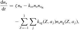 $$\begin{eqnarray}
\frac{{\rm d}n_s}{{\rm d}t} &=& \zeta n_{\rm n} - k_{{\rm e}s}n_s n_{{\rm e}_{\rm R}} \nonumber \\
&&- \sum _{Z=-1}^1 \sum _j k_{s{\rm g}}(Z,a_j)n_s n_{\rm g}(Z,a_j),
\end{eqnarray}$$
$$\begin{eqnarray}
\frac{{\rm d}n_s}{{\rm d}t} &=& \zeta n_{\rm n} - k_{{\rm e}s}n_s n_{{\rm e}_{\rm R}} \nonumber \\
&&- \sum _{Z=-1}^1 \sum _j k_{s{\rm g}}(Z,a_j)n_s n_{\rm g}(Z,a_j),
\end{eqnarray}$$
 $$\begin{eqnarray}
\frac{{\rm d}n_{{\rm e}_{\rm R}}}{{\rm d}t}&=& \zeta n_{\rm n} - \sum _s k_{{\rm e}s}n_s n_{{\rm e}_{\rm R}} \nonumber \\
&&- \sum _{Z=-1}^1 \sum _j k_{\rm eg}(Z,a_j)n_{{\rm e}_{\rm R}}n_{\rm g}(Z,a_j),
\end{eqnarray}$$
$$\begin{eqnarray}
\frac{{\rm d}n_{{\rm e}_{\rm R}}}{{\rm d}t}&=& \zeta n_{\rm n} - \sum _s k_{{\rm e}s}n_s n_{{\rm e}_{\rm R}} \nonumber \\
&&- \sum _{Z=-1}^1 \sum _j k_{\rm eg}(Z,a_j)n_{{\rm e}_{\rm R}}n_{\rm g}(Z,a_j),
\end{eqnarray}$$
 $$\begin{eqnarray}
\frac{{\rm d}n_{\rm g}(Z,a_j)}{{\rm d}t}&=& \ -\sum _s \left[k_{s{\rm g}}(Z,a_j)n_s n_{\rm g}(Z,a_j) \right. \nonumber \\
&&- \left.k_{s{\rm g}}(Z-1,a_j)n_s n_{\rm g}(Z-1,a_j) \right] \nonumber \\
&&- k_{{\rm eg}}(Z,a_j)n_{\rm e} n_{\rm g}(Z,a_j) \nonumber \\
&&+ k_{{\rm eg}}(Z+1,a_j)n_{\rm e} n_{\rm g}(Z+1,a_j),
\end{eqnarray}$$
$$\begin{eqnarray}
\frac{{\rm d}n_{\rm g}(Z,a_j)}{{\rm d}t}&=& \ -\sum _s \left[k_{s{\rm g}}(Z,a_j)n_s n_{\rm g}(Z,a_j) \right. \nonumber \\
&&- \left.k_{s{\rm g}}(Z-1,a_j)n_s n_{\rm g}(Z-1,a_j) \right] \nonumber \\
&&- k_{{\rm eg}}(Z,a_j)n_{\rm e} n_{\rm g}(Z,a_j) \nonumber \\
&&+ k_{{\rm eg}}(Z+1,a_j)n_{\rm e} n_{\rm g}(Z+1,a_j),
\end{eqnarray}$$
where s ∈ {iR, IR}, ζ is the ionisation rate, kij are the charge capture rates, and we set n g(Z = ±2, aj ) ≡ 0 since their populations will be small compared the singly charged grains. Although we only include two ion species for simplicity and performance, it is possible to expand this network to include an arbitrary number of molecular ions.
The ion–electron charge capture rates are given by (Umebayashi & Nakano Reference Umebayashi and Nakano1990)
 $$\begin{eqnarray}
k_{\rm ei} &=& \left[ 3.5 X \left(\frac{T}{300}\right)^{-0.7} + 4.5 Y \left(\frac{T}{300}\right)^{-0.67}\right] \nonumber \\
&&\times 10^{-12}\, {\rm cm}^3\,{\rm s}^{-1}
\end{eqnarray}$$
$$\begin{eqnarray}
k_{\rm ei} &=& \left[ 3.5 X \left(\frac{T}{300}\right)^{-0.7} + 4.5 Y \left(\frac{T}{300}\right)^{-0.67}\right] \nonumber \\
&&\times 10^{-12}\, {\rm cm}^3\,{\rm s}^{-1}
\end{eqnarray}$$
 $$\begin{eqnarray}
k_{\rm eI} = 2.8\times 10^{-12}\left(\frac{T}{300}\right)^{-0.86} {\rm cm}^3\,{\rm s}^{-1} ,
\end{eqnarray}$$
$$\begin{eqnarray}
k_{\rm eI} = 2.8\times 10^{-12}\left(\frac{T}{300}\right)^{-0.86} {\rm cm}^3\,{\rm s}^{-1} ,
\end{eqnarray}$$
where X and Y are the mass fractions of hydrogen and helium, respectively, used to determine the mass of the light ion. For grains, the charge capture rates are (Fujii et al. Reference Fujii, Okuzumi and Inutsuka2011)
 $$\begin{eqnarray}
k_{s{\rm g}}(Z,a_j) &=& a_j^2 \sqrt{\frac{8\pi k_{\rm B}T}{m_s}}\left\lbrace \begin{array}{l l}\left(1-\frac{Z e^2}{a_j k_{\rm B}T}\right) & \quad{\rm if }\quad Z \le 0\\
\exp \left(\frac{-Z e^2}{a_jk_{\rm B}T}\right) & \quad{\rm if }\quad Z > 0 \end{array}\right. ,
\end{eqnarray}$$
$$\begin{eqnarray}
k_{s{\rm g}}(Z,a_j) &=& a_j^2 \sqrt{\frac{8\pi k_{\rm B}T}{m_s}}\left\lbrace \begin{array}{l l}\left(1-\frac{Z e^2}{a_j k_{\rm B}T}\right) & \quad{\rm if }\quad Z \le 0\\
\exp \left(\frac{-Z e^2}{a_jk_{\rm B}T}\right) & \quad{\rm if }\quad Z > 0 \end{array}\right. ,
\end{eqnarray}$$
 $$\begin{eqnarray}
k_{\rm eg}(Z,a_j) &=&a_j^2 \sqrt{\frac{8\pi k_{\rm B}T}{m_{\rm e}}} \left\lbrace \begin{array}{l l}\exp \left(\frac{Z e^2}{a_j k_{\rm B}T}\right) & \quad{\rm if }\quad Z < 0 \\
\left(1+\frac{Z e^2}{a_j k_{\rm B}T}\right) & \quad{\rm if }\quad Z \ge 0 \end{array}\right.,
\end{eqnarray}$$
$$\begin{eqnarray}
k_{\rm eg}(Z,a_j) &=&a_j^2 \sqrt{\frac{8\pi k_{\rm B}T}{m_{\rm e}}} \left\lbrace \begin{array}{l l}\exp \left(\frac{Z e^2}{a_j k_{\rm B}T}\right) & \quad{\rm if }\quad Z < 0 \\
\left(1+\frac{Z e^2}{a_j k_{\rm B}T}\right) & \quad{\rm if }\quad Z \ge 0 \end{array}\right.,
\end{eqnarray}$$
where k B is the Boltzmann constant, e is the electron charge, m e is the mass of an electron, Z is the charge on the grains, and T is the temperature (where the gas and dust are assumed to be in thermal equilibrium).
From charge neutrality,
 $$\begin{equation}
\sum _s n_s - n_{{\rm e}_{\rm R}} + \sum _{Z=-1}^1 \sum _j Z n_{\rm g}(Z,a_j) = 0,
\end{equation}$$
$$\begin{equation}
\sum _s n_s - n_{{\rm e}_{\rm R}} + \sum _{Z=-1}^1 \sum _j Z n_{\rm g}(Z,a_j) = 0,
\end{equation}$$
and from conservation of grains,
 $$\begin{equation}
n_{\rm g}(a_j) = \sum _{Z=-1}^1 n_{\rm g}(Z,a_j),
\end{equation}$$
$$\begin{equation}
n_{\rm g}(a_j) = \sum _{Z=-1}^1 n_{\rm g}(Z,a_j),
\end{equation}$$
where n g(aj ) is the total grain number density as calculated in (1) or (2).
Following Keith & Wardle (Reference Keith and Wardle2014), we assume that the system is approximately in a steady state system (i.e.
 $\frac{{\rm d}}{{\rm d}t} \approx 0$
). The set of equations, (4)–(6), (11), and (12) represents an over-subscription, thus we remove
$\frac{{\rm d}}{{\rm d}t} \approx 0$
). The set of equations, (4)–(6), (11), and (12) represents an over-subscription, thus we remove
 $\frac{{\rm d}n_{{\rm e}_{\rm R}}}{{\rm d}t}$
and
$\frac{{\rm d}n_{{\rm e}_{\rm R}}}{{\rm d}t}$
and
 $\frac{{\rm d}n_{\rm g}(Z=0,a_j)}{{\rm d}t}$
in favour of charge neutrality and conservation of grains. The number densities are calculated by iteratively solving
$\frac{{\rm d}n_{\rm g}(Z=0,a_j)}{{\rm d}t}$
in favour of charge neutrality and conservation of grains. The number densities are calculated by iteratively solving
 $$\begin{equation}
\bm {n}^{t+1} = \bm {n}^t - \mathbb {J}^{-1}(\bm {n}^t) \bm {f}(\bm {n}^t) = \bm {n}^t - \bm {x}^t,
\end{equation}$$
$$\begin{equation}
\bm {n}^{t+1} = \bm {n}^t - \mathbb {J}^{-1}(\bm {n}^t) \bm {f}(\bm {n}^t) = \bm {n}^t - \bm {x}^t,
\end{equation}$$
where t is the iteration number,
 $\mathbb {J}(\bm {n}^t)$
is the Jacobian, and in the default case,
n
t
= {nt
iR
, nt
IR
, nt
e, n
g
t
(Z = −1), nt
g(Z = 0), n
g
t
(Z = −1)} and
f
(
n
t
) = 0 are
$\mathbb {J}(\bm {n}^t)$
is the Jacobian, and in the default case,
n
t
= {nt
iR
, nt
IR
, nt
e, n
g
t
(Z = −1), nt
g(Z = 0), n
g
t
(Z = −1)} and
f
(
n
t
) = 0 are
 $\lbrace \frac{{\rm d}n_{{\rm i}_{\rm R}}}{{\rm d}t}$
,
$\lbrace \frac{{\rm d}n_{{\rm i}_{\rm R}}}{{\rm d}t}$
,
 $\frac{{\rm d}n_{{\rm I}_{\rm R}}}{{\rm d}t}$
, charge neutrality,
$\frac{{\rm d}n_{{\rm I}_{\rm R}}}{{\rm d}t}$
, charge neutrality,
 $\frac{{\rm d}n_{\rm g}(Z=-1)}{{\rm d}t}$
, grain conservation,
$\frac{{\rm d}n_{\rm g}(Z=-1)}{{\rm d}t}$
, grain conservation,
 $\frac{{\rm d}n_{\rm g}(Z=1)}{{\rm d}t}\rbrace$
. Rather than solving for inverse of the Jacobian, we use LU decomposition of the Jacobian to solve for
x
t
in
$\frac{{\rm d}n_{\rm g}(Z=1)}{{\rm d}t}\rbrace$
. Rather than solving for inverse of the Jacobian, we use LU decomposition of the Jacobian to solve for
x
t
in
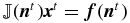 $\mathbb {J}(\bm {n}^t) \bm {x}^t = \bm {f}(\bm {n}^t)$
.
$\mathbb {J}(\bm {n}^t) \bm {x}^t = \bm {f}(\bm {n}^t)$
.
The number densities can span several orders of magnitude, and this method becomes unstable for n g ≫ n e. Although this will likely not be important in most physical applications, an alternative method using average grain charges is described in Appendix D; this method is only used after the above method fails to iterate to a solution within a set number of iterations.
2.2. Thermal ionisation
At high gas temperatures, thermal ionisation can remove electrons. For each species, j, the ion number densities can be calculated using the Saha equation,
 $$\begin{equation}
\frac{n_{{\rm e}_{\rm T}} n_{{\rm i}_{\rm T},j,k+1}}{n_{{\rm i}_{\rm T},j,k}} = \frac{2g_{j,k+1}}{g_{j,k}} \left( \frac{2\pi m_{\rm e} k_{\rm B} T}{h^2}\right)^{3/2} \exp {\left( -\frac{\chi _{j,k+1}}{k_{\rm B}T} \right)},
\end{equation}$$
$$\begin{equation}
\frac{n_{{\rm e}_{\rm T}} n_{{\rm i}_{\rm T},j,k+1}}{n_{{\rm i}_{\rm T},j,k}} = \frac{2g_{j,k+1}}{g_{j,k}} \left( \frac{2\pi m_{\rm e} k_{\rm B} T}{h^2}\right)^{3/2} \exp {\left( -\frac{\chi _{j,k+1}}{k_{\rm B}T} \right)},
\end{equation}$$
where n iT, j, k is the number density of species j which has been ionised k times, χ j, k is the ionisation potential, g j, k is the statistical weight of level k, and h is Planck’s constant. We assume that each atom can be ionised at most twice, thus the total number density of species j will be n iT, j = n iT, j, 0 + n iT, j, 1 + n iT, j, 2, and the number of electrons contributed from species j is n eT, j = n iT, j, 1 + 2n iT, j, 2. Since the number density of each ionisation level of each species can be written as a function of electron number density only, the total electron number density from thermal ionisation is
 $$\begin{equation}
n_{{\rm e}_{\rm T}} = \sum _j \left[n_{{\rm i}_{\rm T},j,1}\left(n_{{\rm e}_{\rm T}} \right) + 2n_{{\rm i}_{\rm T},j,2}\left(n_{{\rm e}_{\rm T}} \right)\right],
\end{equation}$$
$$\begin{equation}
n_{{\rm e}_{\rm T}} = \sum _j \left[n_{{\rm i}_{\rm T},j,1}\left(n_{{\rm e}_{\rm T}} \right) + 2n_{{\rm i}_{\rm T},j,2}\left(n_{{\rm e}_{\rm T}} \right)\right],
\end{equation}$$
which can then be solved iteratively using the Newton-Raphson method. The singly and doubly ionised ions, with number densities n iT, 1 and n iT, 2, respectively, are tracked separately since they have different charges.
The average ion mass is given by Draine & Sutin (Reference Draine and Sutin1987):
 $$\begin{equation}
m_{{\rm i}_{\rm T}} = \left(\frac{n_{{\rm i}_{\rm T},1} + n_{{\rm i}_{\rm T},2}}{\sum _{j,k} \frac{ n_{{\rm i}_{\rm T},j,k} }{ \sqrt{m_{{\rm i}_{\rm T},j}} }}\right)^2,
\end{equation}$$
$$\begin{equation}
m_{{\rm i}_{\rm T}} = \left(\frac{n_{{\rm i}_{\rm T},1} + n_{{\rm i}_{\rm T},2}}{\sum _{j,k} \frac{ n_{{\rm i}_{\rm T},j,k} }{ \sqrt{m_{{\rm i}_{\rm T},j}} }}\right)^2,
\end{equation}$$
where m iT, j is the mass of a particle of species j; note that all ionisation levels are assumed to have the same mass.
In their analytical discussion, Keith & Wardle (Reference Keith and Wardle2014) account for the possibility that dust grains absorb electrons. Similar to cosmic ray ionisation, this would lead to a reduction in the electron number density and a population of negatively charged grains. However, electron absorption by grains is not currently included in our thermal ionisation model. At high temperatures, the grains absorb less than a few percent of the electrons, thus do not contribute meaningfully to n eT . At low temperatures, Z iT = 0 since n eT = 0, but numerical round-off error leads to Z iT ≈ 0, which then gives non-sensical results of the electron number density. Given the physical irrelevance and numerical difficulties at high and low temperatures, respectively, electron absorption is not included in this version of Nicil.
2.3. Charged species populations
Both cosmic ray and thermal ionisation are calculated independently of one another for numerical stability and efficiency. This results in two disconnected free electron populations, and the total electron number density is given by n e = n eR + n eT . As will be shown in Section 3, one ionisation process typically dominates the other, thus our method is reasonable.
The ionisation processes yield seven charged populations:
-
1. free electrons with mass m e, number density n e, and charge Z e ≡ −1,
-
2. light ions from cosmic ray ionisation with mass m iR , number density n iR , and charge Z iR = 1,
-
3. metallic ions from cosmic ray ionisation with mass m IR , number density n IR , and charge Z IR = 1,
-
4. singly ionised ions from thermal ionisation with mass m iT , number density n iT, 1, and charge Z iT, 1 = 1,
-
5. doubly ionised ions from thermal ionisation with mass m iT , number density n iT, 2, and charge Z iT, 2 = 2,
-
6. charged grains from cosmic ray ionisation with mass m g, number density n g(Z = −1), and charge Z g = −1.
-
7. charged grains from cosmic ray ionisation with mass m g, number density n g(Z = 1), and charge Z g = +1.
These species are defined with subscripts e, iR, IR, iT, 1, iT, 2, and g, respectively, where the latter will be used generally for all grain populations. The density of neutral particles is
 $$\begin{eqnarray}
\rho _{\rm n} &=& \rho - \left(\rho _{{\rm i}_{\rm R}} + \rho _{{\rm I}_{\rm R}} + \rho _{{\rm i}_{\rm T}} + \rho _{\rm e}\right), \nonumber\\
&=& \rho - \left[n_{{\rm i}_{\rm R}}m_{{\rm i}_{\rm R}} + n_{{\rm I}_{\rm R}}m_{{\rm I}_{\rm R}} + \left(n_{{\rm i}_{\rm T},1} + n_{{\rm i}_{\rm T},2}\right)m_{{\rm i}_{\rm T}} + n_{\rm e}m_{\rm e}\right].
\end{eqnarray}$$
$$\begin{eqnarray}
\rho _{\rm n} &=& \rho - \left(\rho _{{\rm i}_{\rm R}} + \rho _{{\rm I}_{\rm R}} + \rho _{{\rm i}_{\rm T}} + \rho _{\rm e}\right), \nonumber\\
&=& \rho - \left[n_{{\rm i}_{\rm R}}m_{{\rm i}_{\rm R}} + n_{{\rm I}_{\rm R}}m_{{\rm I}_{\rm R}} + \left(n_{{\rm i}_{\rm T},1} + n_{{\rm i}_{\rm T},2}\right)m_{{\rm i}_{\rm T}} + n_{\rm e}m_{\rm e}\right].
\end{eqnarray}$$
2.4. Conductivities
The conductivities are calculated under the assumption that the fluid evolves on a timescale longer than the collision timescale of any charged particle. The collisional frequencies, ν, are empirically calculated rates for charged species. The electron-ion rate is (Pandey & Wardle Reference Pandey and Wardle2008)
 $$\begin{equation}
\nu _{\rm ei} = 51 \ {\rm s}^{-1} \left(\frac{n_{\rm e}}{{\rm cm}^{-3}}\right)\left(\frac{T}{{\rm K}}\right)^{-3/2},
\end{equation}$$
$$\begin{equation}
\nu _{\rm ei} = 51 \ {\rm s}^{-1} \left(\frac{n_{\rm e}}{{\rm cm}^{-3}}\right)\left(\frac{T}{{\rm K}}\right)^{-3/2},
\end{equation}$$
and the ion–electron rate is
 $\nu _{\rm ie} = \frac{\rho _{\rm e}}{\rho _{\rm i}}\nu _{\rm ei}$
. Note that νeiR
= νeIR
= νeiT, 1 = νeiT, 2 ≡ νei because there is no dependence on ion properties, and νiRe ≠ νiTe.
$\nu _{\rm ie} = \frac{\rho _{\rm e}}{\rho _{\rm i}}\nu _{\rm ei}$
. Note that νeiR
= νeIR
= νeiT, 1 = νeiT, 2 ≡ νei because there is no dependence on ion properties, and νiRe ≠ νiTe.
The plasma-neutral collisional frequency is
 $$\begin{equation}
\nu _{j{\rm n}} = \frac{\left< \sigma v\right>_{j{\rm n}}}{m_{\rm n}+m_j}\rho _{\rm n},
\end{equation}$$
$$\begin{equation}
\nu _{j{\rm n}} = \frac{\left< \sigma v\right>_{j{\rm n}}}{m_{\rm n}+m_j}\rho _{\rm n},
\end{equation}$$
where < σv > jn is the rate coefficient for the momentum transfer by the collision of particle of species j with the neutrals. For electron-neutral collisions, it is assumed that the neutrals are comprised of hydrogen and helium, since these two elements should dominate any physical system. The rate coefficient is then given by
 $$\begin{equation}
\left< \sigma v\right>_{\rm en} = X_{{\rm H}_2} \left< \sigma v\right>_{{\rm e-H}_2} + X_{\rm H} \left< \sigma v\right>_{{\rm e-H}} + Y \left< \sigma v\right>_{\rm e-He},
\end{equation}$$
$$\begin{equation}
\left< \sigma v\right>_{\rm en} = X_{{\rm H}_2} \left< \sigma v\right>_{{\rm e-H}_2} + X_{\rm H} \left< \sigma v\right>_{{\rm e-H}} + Y \left< \sigma v\right>_{\rm e-He},
\end{equation}$$
where X H2 , X H, and Y are the mass fractions of molecular and atomic hydrogen and helium, respectively, and X H2 + X H ≡ X; X and Y are free parameters if use_massfrac=.true., otherwise they are calculated from the given abundances. Following Pinto & Galli (Reference Pinto and Galli2008),
 $$\begin{eqnarray}
\left< \sigma v\right>_{{\rm e-H}_2} &=& \left(0.535+0.203\theta -0.163\theta ^2+0.050\theta ^3\right) \times 10^{-9} \nonumber \\
&& \times\, T^{1/2} \ {\rm cm}^3 \ {\rm s}^{-1} ,
\end{eqnarray}$$
$$\begin{eqnarray}
\left< \sigma v\right>_{{\rm e-H}_2} &=& \left(0.535+0.203\theta -0.163\theta ^2+0.050\theta ^3\right) \times 10^{-9} \nonumber \\
&& \times\, T^{1/2} \ {\rm cm}^3 \ {\rm s}^{-1} ,
\end{eqnarray}$$
 $$\begin{eqnarray}
\left< \sigma v\right>_{{\rm e-H}} &=& \left(2.841+0.093\theta -0.245\theta ^2+0.089\theta ^3\right) \times 10^{-9} \nonumber \\
&& \times\, T^{1/2} \ {\rm cm}^3 \ {\rm s}^{-1} ,
\end{eqnarray}$$
$$\begin{eqnarray}
\left< \sigma v\right>_{{\rm e-H}} &=& \left(2.841+0.093\theta -0.245\theta ^2+0.089\theta ^3\right) \times 10^{-9} \nonumber \\
&& \times\, T^{1/2} \ {\rm cm}^3 \ {\rm s}^{-1} ,
\end{eqnarray}$$
 $$\begin{eqnarray}
\left< \sigma v\right>_{\rm e-He} &=& 0.428 \times 10^{-9} T^{1/2} \ {\rm cm}^3 \ {\rm s}^{-1},
\end{eqnarray}$$
$$\begin{eqnarray}
\left< \sigma v\right>_{\rm e-He} &=& 0.428 \times 10^{-9} T^{1/2} \ {\rm cm}^3 \ {\rm s}^{-1},
\end{eqnarray}$$
where θ ≡ log T for T in K and the drift velocity is assumed to be zero.
The ion-neutral rate is (Pinto & Galli Reference Pinto and Galli2008)
 $$\begin{eqnarray}
\left< \sigma v\right>_{\rm in} &=& 2.81\times 10^{-9} \ {\rm cm}^3 \ {\rm s}^{-1} \nonumber \\
&&\times \left|Z_{\rm i}\right|^{1/2}\left[ X_{{\rm H}_2}\left(\frac{p_{{\rm H}_2}}{{\rm \AA}^3}\right)^{1/2}\left(\frac{\mu _{{\rm i-H}_2}}{m_{\rm p}}\right)^{-1/2} \right. \nonumber \\
&&+ \left. X_{{\rm H}}\left(\frac{p_{{\rm H}}}{{\rm \AA}^3}\right)^{1/2}\left(\frac{\mu _{{\rm i-H}}}{m_{\rm p}}\right)^{-1/2} \right. \nonumber \\
&&+ \left. Y \left(\frac{p_{\rm He}}{{\rm \AA}^3}\right)^{1/2}\left(\frac{\mu _{\rm i-He}}{m_{\rm p}}\right)^{-1/2} \right],
\end{eqnarray}$$
$$\begin{eqnarray}
\left< \sigma v\right>_{\rm in} &=& 2.81\times 10^{-9} \ {\rm cm}^3 \ {\rm s}^{-1} \nonumber \\
&&\times \left|Z_{\rm i}\right|^{1/2}\left[ X_{{\rm H}_2}\left(\frac{p_{{\rm H}_2}}{{\rm \AA}^3}\right)^{1/2}\left(\frac{\mu _{{\rm i-H}_2}}{m_{\rm p}}\right)^{-1/2} \right. \nonumber \\
&&+ \left. X_{{\rm H}}\left(\frac{p_{{\rm H}}}{{\rm \AA}^3}\right)^{1/2}\left(\frac{\mu _{{\rm i-H}}}{m_{\rm p}}\right)^{-1/2} \right. \nonumber \\
&&+ \left. Y \left(\frac{p_{\rm He}}{{\rm \AA}^3}\right)^{1/2}\left(\frac{\mu _{\rm i-He}}{m_{\rm p}}\right)^{-1/2} \right],
\end{eqnarray}$$
where p H2 , p H, and p He are the polarisabilities (Osterbrock Reference Osterbrock1961). This term is calculated independently for each ion due to the ion mass dependence in the reduced masses, μi-H2 , μi-H, and μi-He.
For grain-neutral collisions, the rate coefficient is (Wardle & Ng Reference Wardle and Ng1999; Pinto & Galli Reference Pinto and Galli2008)
 $$\begin{equation}
\left< \sigma v\right>_{\rm gn} = \pi a_{\rm g}^2\delta _{\rm gn}\sqrt{\frac{128k_{\rm B}T}{9\pi m_{\rm n}}},
\end{equation}$$
$$\begin{equation}
\left< \sigma v\right>_{\rm gn} = \pi a_{\rm g}^2\delta _{\rm gn}\sqrt{\frac{128k_{\rm B}T}{9\pi m_{\rm n}}},
\end{equation}$$
where δgn is the Epstein coefficient, and
 $$\begin{equation}
m_{\rm n} = \left(\frac{X}{m_{{\rm H}_2}}+ \frac{Y}{m_{\rm He}} + \sum _k \frac{Z_k}{m_k}\right)^{-1}
\end{equation}$$
$$\begin{equation}
m_{\rm n} = \left(\frac{X}{m_{{\rm H}_2}}+ \frac{Y}{m_{\rm He}} + \sum _k \frac{Z_k}{m_k}\right)^{-1}
\end{equation}$$
is the mass of the neutral particle, where we sum over all included metals, k (if use_massfrac=.false.), which have mass fractions Zk and masses mk . This is the only instance in this paper where Z does not refer to charge. Since m n is a characteristic mass, we assume that all the hydrogen is molecular hydrogen, which is reasonable for low temperatures.
The Hall parameter for species j is given by
 $$\begin{equation}
\beta _j = \frac{|Z_j|eB}{m_j c}\frac{1}{\nu _{j{\rm n}}}.
\end{equation}$$
$$\begin{equation}
\beta _j = \frac{|Z_j|eB}{m_j c}\frac{1}{\nu _{j{\rm n}}}.
\end{equation}$$
A modified form is presented in Appendix E.
Finally, the Ohmic, Hall, and Pedersen conductivities are given by (e.g. Wardle & Ng Reference Wardle and Ng1999; Wardle Reference Wardle2007)
 $$\begin{eqnarray}
\sigma _{\rm O} &=& \frac{ec}{B}\sum _j n_j|Z_j|\beta _j,
\end{eqnarray}$$
$$\begin{eqnarray}
\sigma _{\rm O} &=& \frac{ec}{B}\sum _j n_j|Z_j|\beta _j,
\end{eqnarray}$$
 $$\begin{eqnarray}
\sigma _{\rm H} &=& \frac{ec}{B}\sum _j \frac{n_j Z_j}{1+ \beta _j^2},
\end{eqnarray}$$
$$\begin{eqnarray}
\sigma _{\rm H} &=& \frac{ec}{B}\sum _j \frac{n_j Z_j}{1+ \beta _j^2},
\end{eqnarray}$$
 $$\begin{eqnarray}
\sigma _{\rm P} &=& \frac{ec}{B}\sum _j \frac{n_j |Z_j| \beta _j}{1+ \beta _j^2}.
\end{eqnarray}$$
$$\begin{eqnarray}
\sigma _{\rm P} &=& \frac{ec}{B}\sum _j \frac{n_j |Z_j| \beta _j}{1+ \beta _j^2}.
\end{eqnarray}$$
We explicitly note that σO and σP are positive, whereas σH can be positive or negative. The total conductivity perpendicular to the magnetic field is
 $$\begin{equation}
\sigma _\bot = \sqrt{\sigma _{\rm H}^2 + \sigma _{\rm P}^2}.
\end{equation}$$
$$\begin{equation}
\sigma _\bot = \sqrt{\sigma _{\rm H}^2 + \sigma _{\rm P}^2}.
\end{equation}$$
2.5. Non-ideal MHD coefficients
The induction equation in MHD is
 $$\begin{equation}
\frac{{\rm d} \bm {B}}{{\rm d} t} = \left(\bm {B}\cdot \bm {\nabla }\right)\bm {v}-\bm {B}\left(\bm {\nabla }\cdot \bm {v}\right) + \left.\frac{{\rm d} \bm {B}}{{\rm d} t}\right|_{\rm non-ideal},
\end{equation}$$
$$\begin{equation}
\frac{{\rm d} \bm {B}}{{\rm d} t} = \left(\bm {B}\cdot \bm {\nabla }\right)\bm {v}-\bm {B}\left(\bm {\nabla }\cdot \bm {v}\right) + \left.\frac{{\rm d} \bm {B}}{{\rm d} t}\right|_{\rm non-ideal},
\end{equation}$$
where
 $ \left.\frac{{\rm d} \bm {B}}{{\rm d} t}\right|_{\rm non-ideal}$
is the non-ideal MHD term, which is the sum of Ohmic resistivity (OR), the Hall effect (HE), and ambipolar diffusion (AD) terms; these terms are given by
$ \left.\frac{{\rm d} \bm {B}}{{\rm d} t}\right|_{\rm non-ideal}$
is the non-ideal MHD term, which is the sum of Ohmic resistivity (OR), the Hall effect (HE), and ambipolar diffusion (AD) terms; these terms are given by
 $$\begin{eqnarray}
\left.\frac{{\rm d} \bm {B}}{{\rm d} t}\right|_{\rm OR} &=& -\bm {\nabla } \times \left[ \eta _{\rm OR} \left(\bm {\nabla }\times \bm {B}\right)\right],
\end{eqnarray}$$
$$\begin{eqnarray}
\left.\frac{{\rm d} \bm {B}}{{\rm d} t}\right|_{\rm OR} &=& -\bm {\nabla } \times \left[ \eta _{\rm OR} \left(\bm {\nabla }\times \bm {B}\right)\right],
\end{eqnarray}$$
 $$\begin{eqnarray}
\left.\frac{{\rm d} \bm {B}}{{\rm d} t}\right|_{\rm HE} &=& -\bm {\nabla } \times \left[ \eta _{\rm HE} \left(\bm {\nabla }\times \bm {B}\right)\times \bm {\hat{B}}\right],
\end{eqnarray}$$
$$\begin{eqnarray}
\left.\frac{{\rm d} \bm {B}}{{\rm d} t}\right|_{\rm HE} &=& -\bm {\nabla } \times \left[ \eta _{\rm HE} \left(\bm {\nabla }\times \bm {B}\right)\times \bm {\hat{B}}\right],
\end{eqnarray}$$
 $$\begin{eqnarray}
\left.\frac{{\rm d} \bm {B}}{{\rm d} t}\right|_{\rm AD} &=& \bm {\nabla } \times \left\lbrace \eta _{\rm AD}\left[\left(\bm {\nabla }\times \bm {B}\right)\times \bm {\hat{B}}\right]\times \bm {\hat{B}}\right\rbrace ,
\end{eqnarray}$$
$$\begin{eqnarray}
\left.\frac{{\rm d} \bm {B}}{{\rm d} t}\right|_{\rm AD} &=& \bm {\nabla } \times \left\lbrace \eta _{\rm AD}\left[\left(\bm {\nabla }\times \bm {B}\right)\times \bm {\hat{B}}\right]\times \bm {\hat{B}}\right\rbrace ,
\end{eqnarray}$$
where the use of the magnetic unit vector,
 $\bm {\hat{B}}$
, is to ensure that all three coefficients, η, have units of area per time.
$\bm {\hat{B}}$
, is to ensure that all three coefficients, η, have units of area per time.
From conservation of energy, the contribution to internal energy, u, from the non-ideal MHD terms (Wurster, Price, & Ayliffe Reference Wurster, Price and Ayliffe2014) is
 $$\begin{eqnarray}
\left.\frac{{\rm d} u}{{\rm d} t}\right|_{\rm OR} &=& - \frac{\eta _{\rm OR}}{\rho }\bm {J}\cdot \bm {J} = - \frac{\eta _{\rm OR}}{\rho } J^2,
\end{eqnarray}$$
$$\begin{eqnarray}
\left.\frac{{\rm d} u}{{\rm d} t}\right|_{\rm OR} &=& - \frac{\eta _{\rm OR}}{\rho }\bm {J}\cdot \bm {J} = - \frac{\eta _{\rm OR}}{\rho } J^2,
\end{eqnarray}$$
 $$\begin{eqnarray}
\left.\frac{{\rm d} u}{{\rm d} t}\right|_{\rm HE} &=& - \frac{\eta _{\rm HE}}{\rho }\left(\bm {J}\times \hat{\bm {B}}\right)\cdot \bm {J} = 0,
\end{eqnarray}$$
$$\begin{eqnarray}
\left.\frac{{\rm d} u}{{\rm d} t}\right|_{\rm HE} &=& - \frac{\eta _{\rm HE}}{\rho }\left(\bm {J}\times \hat{\bm {B}}\right)\cdot \bm {J} = 0,
\end{eqnarray}$$
 $$\begin{eqnarray}
\left.\frac{{\rm d} u}{{\rm d} t}\right|_{\rm AD} &=& - \frac{\eta _{\rm AD}}{\rho }\left[\left(\bm {J}\times \hat{\bm {B}}\right)\times \hat{\bm {B}}\right]\cdot \bm {J} \nonumber\\
&=& - \frac{\eta _{\rm AD}}{\rho }\left[\left(\bm {J}\cdot \hat{\bm {B}}\right)^2 - J^2\right].
\end{eqnarray}$$
$$\begin{eqnarray}
\left.\frac{{\rm d} u}{{\rm d} t}\right|_{\rm AD} &=& - \frac{\eta _{\rm AD}}{\rho }\left[\left(\bm {J}\times \hat{\bm {B}}\right)\times \hat{\bm {B}}\right]\cdot \bm {J} \nonumber\\
&=& - \frac{\eta _{\rm AD}}{\rho }\left[\left(\bm {J}\cdot \hat{\bm {B}}\right)^2 - J^2\right].
\end{eqnarray}$$
Next, we invoke the strong coupling approximation, which allows the medium to be treated using the single fluid approximation. It is assumed that the ion pressure and momentum are negligible compared to that of the neutrals, i.e. ρ ~ ρn and ρi ≪ ρ, where ρ, ρn and ρi are the total, neutral, and ion mass densities, respectively.
The general form of the coefficients (Wardle Reference Wardle2007) is
 $$\begin{eqnarray}
\eta _{\rm OR} &=& \frac{c^2}{4\pi \sigma _{\rm O}},
\end{eqnarray}$$
$$\begin{eqnarray}
\eta _{\rm OR} &=& \frac{c^2}{4\pi \sigma _{\rm O}},
\end{eqnarray}$$
 $$\begin{eqnarray}
\eta _{\rm HE} &=& \frac{c^2}{4\pi \sigma _\bot }\frac{\sigma _{\rm H}}{\sigma _\bot },
\end{eqnarray}$$
$$\begin{eqnarray}
\eta _{\rm HE} &=& \frac{c^2}{4\pi \sigma _\bot }\frac{\sigma _{\rm H}}{\sigma _\bot },
\end{eqnarray}$$
 $$\begin{eqnarray}
\eta _{\rm AD} &=& \frac{c^2}{4\pi \sigma _\bot }\frac{\sigma _{\rm P}}{\sigma _\bot } - \eta _{\rm OR} \nonumber \\
&=& \frac{c^2}{4\pi \sigma _{\rm O}}\frac{\sigma _{\rm O}\sigma _{\rm P} - \sigma _\bot ^2}{\sigma _\bot ^2} \equiv \frac{c^2}{4\pi \sigma _{\rm O}}\frac{\sigma _{\rm A}}{\sigma _\bot ^2}.
\end{eqnarray}$$
$$\begin{eqnarray}
\eta _{\rm AD} &=& \frac{c^2}{4\pi \sigma _\bot }\frac{\sigma _{\rm P}}{\sigma _\bot } - \eta _{\rm OR} \nonumber \\
&=& \frac{c^2}{4\pi \sigma _{\rm O}}\frac{\sigma _{\rm O}\sigma _{\rm P} - \sigma _\bot ^2}{\sigma _\bot ^2} \equiv \frac{c^2}{4\pi \sigma _{\rm O}}\frac{\sigma _{\rm A}}{\sigma _\bot ^2}.
\end{eqnarray}$$
The value of η depends on the microphysics of the model, and ηHE can be either positive or negative, whereas ηOR and ηAD are positive (e.g. Wardle & Ng Reference Wardle and Ng1999). To prevent ηAD ≲ 0 due to numerical round-off when σOσP ≈ σ2 ⊥, we use
 $$\begin{eqnarray}
\sigma _{\rm O}\sigma _{\rm P} - \sigma _\bot ^2 &\equiv & \sigma _{\rm A} \nonumber \\
&=& \left(\frac{ec}{B}\right)^2\sum _{j>k} \left[ \frac{ n_j|Z_j|\beta _j}{1+\beta _j^2}\frac{n_k|Z_k|\beta _k}{1+\beta _k^2}\right. \nonumber \\
&&\times \, \left.\left(\frac{Z_k\beta _k}{|Z_k|} - \frac{Z_j\beta _j}{|Z_j|}\right)^2\right],
\end{eqnarray}$$
$$\begin{eqnarray}
\sigma _{\rm O}\sigma _{\rm P} - \sigma _\bot ^2 &\equiv & \sigma _{\rm A} \nonumber \\
&=& \left(\frac{ec}{B}\right)^2\sum _{j>k} \left[ \frac{ n_j|Z_j|\beta _j}{1+\beta _j^2}\frac{n_k|Z_k|\beta _k}{1+\beta _k^2}\right. \nonumber \\
&&\times \, \left.\left(\frac{Z_k\beta _k}{|Z_k|} - \frac{Z_j\beta _j}{|Z_j|}\right)^2\right],
\end{eqnarray}$$
where all pairs of charged species, j and k, are summed over (M. Wardle, private communication 2014).
The non-ideal MHD terms constrain the timestep by
 $$\begin{equation}
{\rm d}t < C_{\rm non-ideal}\frac{h^2}{|\eta |},
\end{equation}$$
$$\begin{equation}
{\rm d}t < C_{\rm non-ideal}\frac{h^2}{|\eta |},
\end{equation}$$
where h is the particle smoothing length or the cell size, η = max (ηOR, |ηHE|, ηAD) and C
non-ideal < 1 is a positive coefficient analogous to the Courant number. Stability tests by Bai (Reference Bai2014) suggest
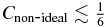 $C_{\rm non\hbox{-}ideal} \lesssim \frac{1}{6}$
is required, whilst wave calculations and tests by Wurster et al. (Reference Wurster, Price and Bate2016) suggest
$C_{\rm non\hbox{-}ideal} \lesssim \frac{1}{6}$
is required, whilst wave calculations and tests by Wurster et al. (Reference Wurster, Price and Bate2016) suggest
 $C_{\rm non\hbox{-}ideal} \lesssim \frac{1}{2\pi }$
is required for stability. Thus, stability can be achieved by choosing a value of C
non-ideal appropriate for a conditionally stable algorithm.
$C_{\rm non\hbox{-}ideal} \lesssim \frac{1}{2\pi }$
is required for stability. Thus, stability can be achieved by choosing a value of C
non-ideal appropriate for a conditionally stable algorithm.
3 TESTS PROGRAMMES AND RESULTS
The Nicil library includes two stand-alone test codes, which can be used to test the effects of varying the parameters. Both can be compiled by typing make in the NICIL directory. This yields the executables nicil_ex_eta and nicil_ex_sph. The latter is a simple SPH code that is primarily used to demonstrate how Nicil is to be implemented into an existing code.
The test programme nicil_ex_eta will calculate the non-ideal MHD coefficients, and output them and the constituent components that are required for their calculation, including number densities of all the charged species and elements, the conductivities, and the coefficients. By default, it outputs three sets of data: one over a range of densities assuming a constant temperature, one over a range of temperatures assuming a constant density, and one where temperature and density are related through the barotropic equation of state (Machida, Inutsuka, & Matsumoto Reference Machida, Inutsuka and Matsumoto2006):
 $$\begin{equation}
T = T_0\sqrt{1+\left(\frac{n}{n_1}\right)^{2\Gamma _1}}\left(1+\frac{n}{n_2}\right)^{\Gamma _2}\left(1+\frac{n}{n_3}\right)^{\Gamma _3},
\end{equation}$$
$$\begin{equation}
T = T_0\sqrt{1+\left(\frac{n}{n_1}\right)^{2\Gamma _1}}\left(1+\frac{n}{n_2}\right)^{\Gamma _2}\left(1+\frac{n}{n_3}\right)^{\Gamma _3},
\end{equation}$$
where T 0 = 10 K, n is the total density, n 1 = 1011, n 2 = 1016, and n 3 = 1021 cm−3, Γ1 = 0.4, Γ2 = −0.3, and Γ3 = 0.56667; the fixed temperature and density for the first two data sets can be modified in src/ nicil_ex_eta.F90. When a magnetic field is required for the constant density and temperature plots, for the purpose of illustration, we use the relation used in Wardle & Ng (Reference Wardle and Ng1999):
 $$\begin{equation}
\left(\frac{B}{{\rm mG}}\right) = \left\lbrace \begin{array}{l l}\left(\frac{n_{\rm n}}{10^6 {\rm cm}^{-3}}\right)^{1/2}; & n_{\rm n} < 10^6 {\rm cm}^{-3} \\
\left(\frac{n_{\rm n}}{10^6 {\rm cm}^{-3}}\right)^{1/4}; & {\rm else} \end{array}\right..
\end{equation}$$
$$\begin{equation}
\left(\frac{B}{{\rm mG}}\right) = \left\lbrace \begin{array}{l l}\left(\frac{n_{\rm n}}{10^6 {\rm cm}^{-3}}\right)^{1/2}; & n_{\rm n} < 10^6 {\rm cm}^{-3} \\
\left(\frac{n_{\rm n}}{10^6 {\rm cm}^{-3}}\right)^{1/4}; & {\rm else} \end{array}\right..
\end{equation}$$
When a magnetic field is required for the barotropic equation of state, we use (Li et al. Reference Li, Krasnopolsky and Shang2011)
 $$\begin{equation}
\left(\frac{B}{{\rm G}}\right) = 1.34 \times 10^{-7} \sqrt{n_{\rm n}}.
\end{equation}$$
$$\begin{equation}
\left(\frac{B}{{\rm G}}\right) = 1.34 \times 10^{-7} \sqrt{n_{\rm n}}.
\end{equation}$$
Figure 1 shows the output of nicil_ex_eta using the default options listed in Table A2; the left-hand plot shows the results using T = 30 K and T ≡ T(n) as a function of density, and the right-hand plot shows the results using ρ = 10−13 g cm−3 and n ≡ n(T) as a function of temperature.
Top to bottom: Charged species number densities, charged element number densities, conductivities, and non-ideal MHD coefficients. The first and second columns use T = 30 K and T ≡ T(n), respectively, plotted as a function of number density (bottom tics) and mass density (top tics), and the third and fourth columns use ρ = 10−13 g cm−3 and n ≡ n(T) plotted as a function of temperature. The second and fourth columns are generated from the same data. This test was performed using Version 1.2.1 of Nicil and the default options listed in Table A2.

For constant T = 30 K, the trends for the ion and electron number densities and the conductivities are in approximate agreement with Wardle & Ng (Reference Wardle and Ng1999); differences arise as a result of different initial conditions and assumptions. The elemental number densities are zero, as is expected at such a low temperature. At this temperature, the conductivities and non-ideal MHD coefficients are strongly dependent on density, whilst the grain charge and ion and electron number densities essentially have two states: one at high density and one at low density.
For constant ρ = 10−13 g cm−3, which is characteristic in discs around protostars, cosmic ray ionisation is the dominant ionisation source for T ≲ 600 K; for T ≳ 600 K, thermal ionisation is the dominant source of electrons. The changeover from the dominance of cosmic ray ionisation to thermal ionisation is abrupt, confirming that the two processes can be calculated independently without loss of information.
These tests were performed using Version 1.2.1 of Nicil, which can be found in commit 8220ec8 from 2016 August 2. The plots can be reproduced using the included Python graphing script, plot_results.py, which calls GNUplot. It is recommended that the user becomes familiar with the effect of the various parameters and processes prior to implementing Nicil into the existing code. This can be done by modifying the parameters (see Section 5.1), plotting them using plot_results.py, and then comparing the new graphs to those made with the default parameters.
4 TEST IN A COLLAPSING MOLECULAR CLOUD
For an astrophysical example, we model the collapse of a rotating, 1 M⊙ cloud of gas using the 3D smoothed particle MHD code Phantom with the inclusion of self-gravity. The cloud has an initial radius of 4 × 1016 cm and is initially threaded with a magnetic field of strength 163 μG (five critical mass-to-flux units) which is anti-aligned with the angular momentum vector. When the maximum density surpasses ρcrit = 10−10 g cm−3 and a given set of criteria are met, the densest gas particle is replaced with a sink particle and its neighbours within r acc = 6.7 AU are immediately accreted onto it. This setup is the same as in Wurster et al. (Reference Wurster, Price and Bate2016), with 106 particles in the cloud.
We ran four tests: Ideal MHD, Nicil with the default settings, using MRN grain size distribution with five bins, and using only cosmic ray ionisation. The face-on gas column density at 1.07 t ff (where the free-fall time is t ff = 2.4 × 10⁴ yr) is shown in Figure 2 for the ideal, default, and MRN models. No discernible disc forms in the ideal MHD model, which demonstrates the magnetic braking catastrophe (e.g. Allen, Li, & Shu (Reference Allen, Li and Shu2003); Price & Bate (Reference Price and Bate2007); Mellon & Li (Reference Mellon and Li2008); Hennebelle & Fromang (Reference Hennebelle and Fromang2008); Wurster et al. Reference Wurster, Price and Bate2016). When the default parameters are used, a weak disc forms around the sink particle. A low-mass disc may also be forming in the MRN model, however, it is difficult to draw conclusions since such a disc will be heavily influenced by the sink particle. At this time, the temperature is less than a few hundred Kelvin, thus thermal ionisation plays a minimal role. As expected, the cosmic ray-only model yields similar results to the default model.
Face-on gas column density of a collapsing 1 M⊙ cloud of gas at 1.07t ff (where the free-fall time is t ff = 2.4 × 10⁴ yr). The magnetic field has a strength of 163 μG (five critical mass-to-flux units) and is initially anti-aligned with the angular momentum vector. From left to right, the models use ideal MHD, use the default Nicil parameters, and use the MRN grain size distribution with five bins. The black circles represents the sink particle with the radius of the circle representing the accretion radius of the sink particle. Each frame is (90 AU)2. There is no discernible disc in the ideal MHD model, whilst the model with the default parameters yield the densest disc.

The radial profiles in the disc of the magnetic field, temperature, and non-ideal MHD coefficients are shown in Figure 3 for the ideal MHD, default, and MRN models. Gas is assumed to be ‘in the disc’, if ρ > ρdisc, min = 10−13 g cm−3.
Radial profiles of the gas with ρ > ρdisc, min = 10−13 g cm−3 at t = 1.07 t ff in the collapsing molecular cloud test. Top to bottom: Magnetic field, mean and maximum temperature, and non-ideal MHD coefficients for the default (solid) and MRN (dashed) models. Since T ≲ 200 K, thermal ionisation plays a negligible role. The coefficients, η, are larger in the default model, and in both cases, ηHE < 0; as a result, the magnetic field strength in the disc increases from the ideal MHD to default to MRN models.

Given that the maximum temperature is typically ≲ 200 K, thermal ionisation plays a negligible role. The coefficients are typically larger in magnitude for the default model, with |ηHE| > ηAD > ηOR. The negative Hall coefficient is responsible for increasing the magnetic field from the ideal MHD to the MRN to the default model.
This MRN grain model includes five bins, and takes 55% longer to reach the t = 1.07 t ff than the default model. Thus, the user must be cautious about performance when using the MRN model.
5 IMPLEMENTATION INTO EXISTING CODE
Nicil is a Fortran90 module that is contained in one file, src/ nicil.F90. To include Nicil in the user’s code, copy this file into the existing code’s source directory and include it in the Makefile, ensuring that nicil.F90 is compiled in double precision; see src/Makefile for details.
The modifications required to the user’s code are summarised below. The Nicil library includes a simple SPH programme, src/ nicil_ex_sph.F90, which can be used as an example.
5.1. Parameter modifications to nicil.F90
The parameters which can be modified by the user are listed at the top of nicil.F90 between the lines labelled ‘Input Parameters,’ and ‘End of Input Parameters.’ These parameters are defined as public, thus can also be modified by other programmes in the user’s code.
If the user wishes to add or remove elements if use_massfrac=.false., then this is done in the subroutine nicil_initial_species. Modify nelements to be the new number of elements, and add the characteristics of the new elements to the relevant arrays, using the current elements as a template.
5.2. Modifications to user’s initialisation subroutine
Nicil contains several variables that require initialising. When defining the variables and subroutines in the existing initialisation subroutine, include
-
use nicil, only : nicil_initialise
-
integer :: ierr .
Once the units are initialised by the existing code, include
-
call nicil_initialise(utime,udist, &umass, unit_Bfield,ierr)
-
if (ierr > 0) & call abort_subroutine_of_user
where utime, udist, umass, and unit_Bfield are unit conversions from CGS to code units. Note that the code unit of temperature is assumed to be Kelvin. If ierr > 0, then an error occurred during initialisation, and the user’s programme should be immediately aborted, using the user’s preferred method (e.g. by calling abort_subroutine_of_user).
The number densities are calculated iteratively, thus the user must define and save these arrays within the body of their code; the number density array for cosmic rays (thermal ionisation) requires four values (one value) for every cell/particle. The user is required to initialise these arrays to zero. For simplicity, they can be treated (i.e. saved and updated) analogously to the user’s existing density array.
5.3. Modifications to user’s density loop
In many codes, the density is calculated prior to calculating the forces and magnetic fields. At the same time, Nicil should calculate the number densities, which do not depend on any neighbours. To calculate the ith element of these arrays, nR and neT, include
-
call nicil_get_ion_n(rho(i),T(i),&
-
nR(1:4,i),neT(i),ierr)
-
if (ierr/=0) then
-
call nicil_translate_error(ierr)
-
if (ierr > 0) call abort_subroutine_of_user
-
end if
in the density loop, where rho(i) and T(i) are the current values of density and temperature, respectively, and nR(1:4,i) and neT(i) are the characteristic number densities from cosmic rays and the electron number density from thermal ionisation, respectively. If an error has occurred, nicil_get_ion_n will return ierr ≠ 0, which will then be passed into nicil_translate_error. If ierr is returned from nicil_translate_error as a negative number, then the error is not fatal; the error message will be written to file if warn_verbose = .true., otherwise all non-fatal errors will be suppressed. If a fatal error message is returned, then it will be printed to file prior to the user executing the existing code’s subroutine to terminate the programme.
The following subroutines and variables need to be imported and defined:
-
use nicil, only : nicil_get_ion_n, &
-
nicil_translate_error
-
integer :: ierr .
5.4. Modifications to user’s magnetic field loop
In the subroutine where the magnetic field is calculated, define
-
use nicil, only : nicil_get_eta, &
-
nicil_translate_error
-
integer:: ierr
-
real:: eta_ohmi, eta_halli, eta_ambii
Then, for each particle/cell i, include
-
call nicil_get_eta(eta_ohmi, &
-
eta_halli,eta_ambii,Bi,rho(i), &T(i),nR(1:4,i),neT(i),ierr)
-
if (ierr/=0) then
-
call nicil_translate_error(ierr)
-
if (ierr > 0) & call abort_subroutine_of_user
-
end if
where eta_ohmi, eta_halli, and eta_ambii are the calculated (i.e. output) non-ideal MHD coefficients, and Bi is the magnitude of the particle/cell’s magnetic field.
With the non-ideal MHD coefficients now calculated, the user can calculate
 $\left.\frac{{\rm d} \bm {B}}{{\rm d} t}\right|_{\rm non\hbox{-}ideal}$
using the existing routines within the user’s code.
$\left.\frac{{\rm d} \bm {B}}{{\rm d} t}\right|_{\rm non\hbox{-}ideal}$
using the existing routines within the user’s code.
5.5. Optional modifications to the user’s code
5.5.1. Timesteps
For each particle/cell, the non-ideal MHD timestep can be calculated by calling
-
call nimhd_get_dt(dtohmi,dthalli, &
-
dtambii,hi, &eta_ohmi,eta_halli,eta_ambii)
where hi is the smoothing length of the particle or the size of the cell, and dtohmi, dthalli, and dtambii are the three output timesteps. These are returned independently in case the user employs a timestepping scheme such as super timestepping (Alexiades, Amiez, & Gremaud Reference Alexiades, Amiez and Gremaud1996), which requires dtohmi and dtambii to be treated differently from dthalli. The timesteps can be calculated with minimal extra cost if the modifications are included in the i-loop after the non-ideal MHD coefficients are already calculated.
5.5.2. Internal energy
Nicil also includes a subroutine that evolves the internal energy of the particle or cell. This is called by
-
call nimhd_get_dudt(dudtnonideal, &
-
eta_ohmi,eta_ambii,rhoi,jcurrenti, &Bxyzi)
where Bxyzi is an array containing the three components of the magnetic field, i.e. (Bxi,Byi,Bzi), and dudtnonideal is the calculated (i.e. output) change in energy for the particle/cell caused by the non-ideal MHD effects.
5.5.3. Ion velocity
The ion velocity is given by
 $$\begin{equation}
\bm {v}_{\rm ion} = \bm {v} + \eta _{\rm AD}\left(\bm {\nabla }\times \hat{B}\right)\times \hat{B},
\end{equation}$$
$$\begin{equation}
\bm {v}_{\rm ion} = \bm {v} + \eta _{\rm AD}\left(\bm {\nabla }\times \hat{B}\right)\times \hat{B},
\end{equation}$$
which can optionally be calculated by calling
-
call nicil_get_vion(eta_ambii,&
-
vxi,vyi,vzi,Bxi,Byi,Bzi,jcurrenti,&
-
vioni,ierr)
where vxi, vyi, vzi, Bxi, Byi, Bzi are the components of the velocity and magnetic field of particle/cell i, and vioni is an output array containing the three components of the ion velocity. Similar to nicil_get_dt, it is optimal to call this array in the i-loop after the non-ideal MHD coefficients are calculated for particle i. Note that ierr is not initialised in this subroutine, thus must either be passed in from nicil_get_eta, or reinitialised before calling this routine. The drift velocity is calculated by
 $$\begin{equation}
\bm {v}_{\rm drift} = \bm {v} - \bm {v}_{\rm ion}.
\end{equation}$$
$$\begin{equation}
\bm {v}_{\rm drift} = \bm {v} - \bm {v}_{\rm ion}.
\end{equation}$$
If warn_verbose = .true., then a warning will be printed if the ion and neutral velocity differ by more than 10%; recall that v drift ≈ 0 is assumed in rate coefficients given in (21)–(23).
5.5.4. Removing if-statements
Given the versatile design of Nicil, the source code contains several if-statements whose argument is a logical operator set prior to runtime. Since these if-statements will be called repeatedly throughout a calculation, their calls may decrease performance of the code if not properly optimised by the compiler. Thus, src/hardcode_ifs.py can be executed in the src/ directory to remove them.
Specifically, this script will read through nicil_source.F90, determine the value of the logical operators, then rewrite nicil.F90 such that every time an if-statement is encountered with a logical operator, the if-statement will be removed, as will its contents if the logical is set to .false.. Note that any changes made to nicil.F90 will be overwritten, thus all parameters must be set in nicil_source.F90 if this script is to be used. The files nicil.F90 and nicil_source.F90 are identical in the repository.
6 CONCLUSION
We have introduced NICIL: Non-Ideal MHD Coefficients and Ionisation Library. This a Fortran90 module that is fully parameterisable to allow the user to determine which processes to include and the values of the parameters. We have described its algorithms, including the cosmic ray and thermal ionisation processes, and how the conductivities and non-ideal MHD coefficients are calculated. We have summarised how to implement Nicil into an existing code.
The library contains two test codes, one of which outputs the non-ideal MHD coefficients and its constituent components. We have described the results using the default values, and showed how the components are affected by temperature and density.
Nicil is a self-contained code that is freely available, and is ready to be implemented in existing codes.
ACKNOWLEDGEMENTS
We would like to thank Daniel Price and Mathew Bate for useful discussions and for their testing and debugging efforts. JW acknowledges support from the Australian Research Council (ARC) Discovery Projects Grant DP130102078 and from the European Research Council under the European Community’s Seventh Framework Programme (FP7/2007–2013 grant agreement no. 339248).
A LIST OF FILES
Table A1 lists and summarises the important files that are included in the Nicil library.
A list of the important files in the Nicil library. The first two files are executables that appear only after Nicil is compiled.

B FREE PARAMETERS
Table A2 lists the free parameters, the default settings, and the reference for the default value (where applicable).
A list of the important parameters in Nicil, along with the default values and references. The first column is the name of the variable in the code, and the actual variable (where it exists) is given in the third column as part of the description.

For use_massfrac = .false., abundances are used in the thermal ionisation calculation. Five elements are included by default, and they, their abundances, and their first and second ionisation potentials are listed in Table A3. The abundance, xj is related to the logarithmic abundance Xj by xj = 10 Xj /(∑ i 10 Xi ).
The default abundances for use_massfrac=.false. (Cox Reference Cox2000; Asplund et al. Reference Asplund, Grevesse, Sauval and Scott2009; Keith & Wardle Reference Keith and Wardle2014).
We initially assume that all of the hydrogen is molecular hydrogen, H2. Using the local temperature and the Saha equation, the number densities of both molecular and atomic hydrogen are determined, viz.,
 $$\begin{equation}
\frac{n_{\rm H} n_{\rm H}}{n_{{\rm H}_2}} = \left[ \frac{2\pi \left( m_{\rm H}m_{\rm H}/m_{{\rm H}_2} \right) k_{\rm B} T}{h^2}\right]^{3/2} \exp {\left( -\frac{\chi _{H-H_2}}{k_{\rm B}T} \right)},
\end{equation}$$
$$\begin{equation}
\frac{n_{\rm H} n_{\rm H}}{n_{{\rm H}_2}} = \left[ \frac{2\pi \left( m_{\rm H}m_{\rm H}/m_{{\rm H}_2} \right) k_{\rm B} T}{h^2}\right]^{3/2} \exp {\left( -\frac{\chi _{H-H_2}}{k_{\rm B}T} \right)},
\end{equation}$$
where χ H − H 2 = 4.476 eV is the dissociation potential and n H + n H2 = A H n 0/2, where A H is the abundance of hydrogen as given in Table A3 and n 0 is the total number density. The mass fractions, X H2 and X H, are then calculated for use in the rate coefficients. For thermal ionisation, we only allow molecular hydrogen to be singly ionised, with an ionisation potential of 15.60 eV.
C CONSTANT NON-IDEAL MHD COEFFICIENTS
In some scenarios, such as test problems, it may be useful to use semi-constant coefficients. To implement this, set eta_constant=.true.; the coefficients then become
 $$\begin{eqnarray}
\eta _{\rm OR} &=& C_{\rm OR},
\end{eqnarray}$$
$$\begin{eqnarray}
\eta _{\rm OR} &=& C_{\rm OR},
\end{eqnarray}$$
 $$\begin{eqnarray}
\eta _{\rm HE} &=& C_{\rm HE}B,
\end{eqnarray}$$
$$\begin{eqnarray}
\eta _{\rm HE} &=& C_{\rm HE}B,
\end{eqnarray}$$
 $$\begin{eqnarray}
\eta _{\rm AD} &=& C_{\rm AD}v_{\rm A}^2 ,
\end{eqnarray}$$
$$\begin{eqnarray}
\eta _{\rm AD} &=& C_{\rm AD}v_{\rm A}^2 ,
\end{eqnarray}$$
where B is the magnitude of the magnetic field and
 $v_{\rm A} = \frac{B}{\sqrt{4\pi \rho }}$
is the Alfvén velocity which are self-consistently calculated, as done during tests of ambipolar diffusion in e.g. Mac Low et al. (Reference Low, Norman, Konigl and Wardle1995), Choi, Kim, & Wiita (Reference Choi, Kim and Wiita2009), and Wurster et al. (Reference Wurster, Price and Ayliffe2014). C is a free parameter to be input by the user. The default values are given in Table A4.
$v_{\rm A} = \frac{B}{\sqrt{4\pi \rho }}$
is the Alfvén velocity which are self-consistently calculated, as done during tests of ambipolar diffusion in e.g. Mac Low et al. (Reference Low, Norman, Konigl and Wardle1995), Choi, Kim, & Wiita (Reference Choi, Kim and Wiita2009), and Wurster et al. (Reference Wurster, Price and Ayliffe2014). C is a free parameter to be input by the user. The default values are given in Table A4.
The free parameters for fixed resistivity coefficients using eta_constant=.true.. The top three parameters are used if eta_const_calc = .false. and the bottom four parameters are used if eta_const_calc = .true..

To calculate the coefficients from fixed parameters that are characteristic of the environment, set
 ${\tt eta\_const\_calc = .true.}$
, and the coefficients become
${\tt eta\_const\_calc = .true.}$
, and the coefficients become
 $$\begin{eqnarray}
\eta _{\rm OR} &=& \frac{m_{\rm e}c^2}{4\pi e^2 n_{\rm e,0}},
\end{eqnarray}$$
$$\begin{eqnarray}
\eta _{\rm OR} &=& \frac{m_{\rm e}c^2}{4\pi e^2 n_{\rm e,0}},
\end{eqnarray}$$
 $$\begin{eqnarray}
\eta _{\rm HE} &=& s_{\rm H} \frac{c}{4\pi e n_{\rm e,0}}B,
\end{eqnarray}$$
$$\begin{eqnarray}
\eta _{\rm HE} &=& s_{\rm H} \frac{c}{4\pi e n_{\rm e,0}}B,
\end{eqnarray}$$
 $$\begin{eqnarray}
\eta _{\rm AD} &=& \frac{1}{4\pi \gamma _{\rm AD} \rho _{\rm i,0}\left(\frac{\rho _{\rm n}}{\rho _{\rm n,0}}\right)^\alpha }v_{\rm A}^2,
\end{eqnarray}$$
$$\begin{eqnarray}
\eta _{\rm AD} &=& \frac{1}{4\pi \gamma _{\rm AD} \rho _{\rm i,0}\left(\frac{\rho _{\rm n}}{\rho _{\rm n,0}}\right)^\alpha }v_{\rm A}^2,
\end{eqnarray}$$
where the free parameters are the fixed electron number density n e, 0, the fixed ion density ρi, 0, the fixed neutral density ρn, 0, the power-law exponent α (α = 0 for molecular cloud densities, and α = 0.5 for low-density regime; c.f. Mac Low et al. Reference Low, Norman, Konigl and Wardle1995), the collisional coupling coefficient for ambipolar diffusion γAD and s H = ±1 is the sign of the Hall coefficient. Invoking the strong coupling approximation, we set ρn = ρ in (A7). The default values are given in Table A4.
Since these forms of the non-ideal MHD coefficients are not self-consistently calculated, it is recommended that eta_constant=.true. be used for testing purposes only.
D APPROXIMATING NUMBER DENSITIES USING AVERAGE GRAIN CHARGES
If NICIL fails to calculate the number densities from cosmic rays using the Jacobian method describe in Section 2.1, then the following method is invoked to approximate the number densities. This method is used with caution since it makes several assumptions. First, it is assumed that n
n ≈ n. Second, it is assumed that recombination rate is small compared to the other processes, thus k
es
= 0. Third, the grains of each size are treated as a single population with an average grain charge of
 $\bar{Z} < 0$
. From (4) and (5), these simplifications allow the ion and electron number densities to be written as
$\bar{Z} < 0$
. From (4) and (5), these simplifications allow the ion and electron number densities to be written as
 $$\begin{eqnarray}
n_s(\bar{Z}) &=& \frac{\zeta n}{\sum _j k_{s{\rm g}}(\bar{Z},a_j) n_{\rm g}(a_j)},
\end{eqnarray}$$
$$\begin{eqnarray}
n_s(\bar{Z}) &=& \frac{\zeta n}{\sum _j k_{s{\rm g}}(\bar{Z},a_j) n_{\rm g}(a_j)},
\end{eqnarray}$$
 $$\begin{eqnarray}
n_{{\rm e}_{\rm R}}(\bar{Z}) &=& \frac{\zeta n}{\sum _j k_{\rm eg}(\bar{Z},a_j) n_{\rm g}(a_j)},
\end{eqnarray}$$
$$\begin{eqnarray}
n_{{\rm e}_{\rm R}}(\bar{Z}) &=& \frac{\zeta n}{\sum _j k_{\rm eg}(\bar{Z},a_j) n_{\rm g}(a_j)},
\end{eqnarray}$$
where s ∈ {iR, IR}. Then, from charge neutrality,
 $$\begin{equation}
\sum _s n_s(\bar{Z}) - n_{{\rm e}_{\rm R}}(\bar{Z}) + \sum _j \bar{Z}n_{\rm g}(a_j) = 0,
\end{equation}$$
$$\begin{equation}
\sum _s n_s(\bar{Z}) - n_{{\rm e}_{\rm R}}(\bar{Z}) + \sum _j \bar{Z}n_{\rm g}(a_j) = 0,
\end{equation}$$
the Newton-Raphson method can be used to solve for
 $\bar{Z}$
. Recall that n
g(aj
) is the total grain number density of grains of size aj
.
$\bar{Z}$
. Recall that n
g(aj
) is the total grain number density of grains of size aj
.
Using
 $\bar{Z}$
, the ion and electron number densities are calculated using (A8) and (A9), respectively. Using (6), charge neutrality and grain conservation, the grain number densities are calculated viz.,
$\bar{Z}$
, the ion and electron number densities are calculated using (A8) and (A9), respectively. Using (6), charge neutrality and grain conservation, the grain number densities are calculated viz.,
 $$\begin{eqnarray}
n_{\rm g}(Z=-1,a_j) &=& \frac{k_{\rm eg}^+n_{\rm e}(1+\bar{Z})n_{\rm g}}{ \sum _s k_{s{\rm g}}^-n_s + k_{\rm eg}^-n_{\rm e} + 2k_{\rm eg}^0n_{\rm e}}
\end{eqnarray}$$
$$\begin{eqnarray}
n_{\rm g}(Z=-1,a_j) &=& \frac{k_{\rm eg}^+n_{\rm e}(1+\bar{Z})n_{\rm g}}{ \sum _s k_{s{\rm g}}^-n_s + k_{\rm eg}^-n_{\rm e} + 2k_{\rm eg}^0n_{\rm e}}
\end{eqnarray}$$
 $$\begin{eqnarray}
n_{\rm g}(Z=+1,a_j) &=& \frac{(1-\bar{Z})n_{\rm g}\sum _s k_{s{\rm g}}^0 n_s }{ \sum _s \left[k_{s{\rm g}}^+ +2k_{s{\rm g}}^0\right]n_s + k_{\rm eg}^+ n_{\rm e} }
\end{eqnarray}$$
$$\begin{eqnarray}
n_{\rm g}(Z=+1,a_j) &=& \frac{(1-\bar{Z})n_{\rm g}\sum _s k_{s{\rm g}}^0 n_s }{ \sum _s \left[k_{s{\rm g}}^+ +2k_{s{\rm g}}^0\right]n_s + k_{\rm eg}^+ n_{\rm e} }
\end{eqnarray}$$
 $$\begin{eqnarray}
n_{\rm g}(Z=0,a_j) &=& n_{\rm g} - n_{\rm g}(Z=-1,a_j) \nonumber \\
&-& n_{\rm g}(Z=1,a_j),
\end{eqnarray}$$
$$\begin{eqnarray}
n_{\rm g}(Z=0,a_j) &=& n_{\rm g} - n_{\rm g}(Z=-1,a_j) \nonumber \\
&-& n_{\rm g}(Z=1,a_j),
\end{eqnarray}$$
where k + ≡ k(Z = 1, aj ), k − ≡ k(Z = −1, aj ) and k 0 ≡ k(Z = 0, aj ).
E MODIFIED HALL PARAMETER
A modified version of the Hall parameter was used in Wurster et al. (Reference Wurster, Price and Bate2016):
 $$\begin{eqnarray}
\beta _{\rm e} &=& \frac{|Z_{\rm e}|eB}{m_{\rm e} c}\frac{1}{\nu _{\rm en}+\nu _{\rm ei}},
\end{eqnarray}$$
$$\begin{eqnarray}
\beta _{\rm e} &=& \frac{|Z_{\rm e}|eB}{m_{\rm e} c}\frac{1}{\nu _{\rm en}+\nu _{\rm ei}},
\end{eqnarray}$$
 $$\begin{eqnarray}
\beta _{\rm i} &=& \frac{|Z_{\rm i}|eB}{m_{\rm i} c}\frac{1}{\nu _{\rm in}+\nu _{\rm ie}}.
\end{eqnarray}$$
$$\begin{eqnarray}
\beta _{\rm i} &=& \frac{|Z_{\rm i}|eB}{m_{\rm i} c}\frac{1}{\nu _{\rm in}+\nu _{\rm ie}}.
\end{eqnarray}$$
With these modifications, the coefficient for Ohmic resistivity from Pandey & Wardle (Reference Pandey and Wardle2008) and Keith & Wardle (Reference Keith and Wardle2014) can be recovered under the assumption βi ≪ βe. By default, these forms are not used, but are included for legacy reasons.


