2. Materials and methods

2.1. Experimental set-up and measurement of weathering crust evolution

Field measurements were conducted at two sites on the western margin of the Greenland ice sheet in the summers of 2022 (∼40 km east of Ilulissat; 69.430° N, −49.866° E) and 2024 (∼2 km east of the S6 weather station on the K-Transect; 67.077° N, −49.337° E; Smeets and others Reference Smeets2018; 1a). In total, five weathering crust ‘reset’ experiments (described below) were conducted to explore the initial formation process of the weathering crust in response to meteorological conditions. Measurement periods were targeted on clear-sky days with no rainfall and otherwise typical summer conditions on the Greenland ice sheet. One experiment was conducted at ILU-22 and four at KAN-24—S15 and WCR 1–4 respectively. The S15 experiment was conducted on Day of Year (DOY) 215 in 2022, WCR1 and 2 experiments on DOY 203 in 2024, and WCR3 and 4 on DOY 209 in 2024. Alongside the targeted reset experiments at ILU-22, opportunistic core collection was conducted between DOYs 206 and 220, on non-reset surfaces. The core processing procedure for these cores was identical to that for the cores collected within the reset experiment.

Figure 1.

A map of Greenland showing the location of the two field sites with insets from Landsat (8 and 9) and a timeline for the reset experiment (a–e). (a) Mechanical clearing of the weathered surface using hand tools; (b) the cleared plot; (c) the >48 hour radiation blocking period, where the plot was covered with solar panels; (d) core extraction*; and (e) core segmenting*. *Note these images are illustrative only and were not taken during the reset experiment.

The ‘reset’ experimental surface was created by the removal of the weathering crust. This was achieved by (a) mechanically removing weathered ice and (b) by manipulating the surface energy balance by blocking incoming SWR. At a 2 × 2 m plot with visibly ‘clean’ ice (i.e. with minimal surface debris, microbes or cryoconite holes) the topmost layer of weathered ice (∼5 cm deep) was removed using hand tools. Subsequently, the experimental surfaces were covered with flexible solar panels for at least 3 days (1b), which was determined as a suitable minimum duration by preliminary observation. The upper ∼1 m of ice at each plot was assumed to be structurally homogenous. The solar panels acted as radiation blockers, preventing SWR from reaching the ice—stopping ongoing weathering—and promoting sensible heat fluxes by warming in response to absorption of SWR. Weathering of the ice surface was initiated by the removal of the solar panels (1c). The success of this approach was validated by ice density measurements immediately following the exposure of the experimental surface (see below)—with measurements indicating bulk ice densities of ∼910 kg m⁻³, equal to unweathered ice (Cuffey and Paterson, Reference Cuffey and Paterson2010).

At each experimental plot, near-surface ice density profiles were measured over either a 22 hour (S15) or 25 hour (KAN-24) period between 1000 and 1100 the following day, with measurements beginning immediately after exposure of the reset surface at ∼1000. The S15 experiment was curtailed following a measurement at 0845, due to rainfall. For all experiments, 12 measurements of ice density were taken, despite the difference in overall duration of the experiments. Quasi-hourly measurements were collected between 1000 and 1600, with less frequent measurements taken outside of this window. Precise sampling times can be seen in the publicly accessible dataset. Albedo was measured only during the hours of 1000 and 1700, to ensure a suitable solar zenith for reliable measurements. Concurrently, hourly averaged meteorological data were collected using either (a) a custom weather station, with capabilities equivalent to that of a PROMICE station (see Fausto and others Reference Fausto2021 and Supplementary Table S1) in 2022, or (b) the S6 weather station in the K-Transect (Smeets and others Reference Smeets2018) in 2024. Briefly, each AWS was equipped with a net radiometer, thermometer, barometer, hygrometer and anemometer. The AWSs collected measurements every 10 min, reporting either hourly (ILU-22) or half-hourly (S6) averages. The ILU-22 AWS operated between DOYs 205–226, while the S6 station is a permanent installation. Surface lowering between the start and end of each experimental period was measured using an ablation stake at the corner of each experimental plot.

A total of 60 depth–density profiles were measured using a volume-gravimetry method: a ∼500 mm deep core was collected using a Kovacs Mark V corer (diameter 140 mm), which was then drained of water and evacuated from the corer barrel. When evacuating the core, a pre-weighed sample bag was placed over the end of the corer to ‘catch’ the upper sections of the core in the event of core collapse. When such core collapse occurred, segment thickness was calculated by subtracting the sum of the stable segments, and the saw blade thickness (multiplied by the number of cuts made), from the hole depth. When the base of the core was not perpendicular to the core edge, this material was simply removed. The solid core was segmented at semi-regular intervals of ∼50 mm—with respect for visual changes within the core—using a power saw. Segments were again drained as completely as practicable to the cessation of active dripping, supported by a visual check of visible pores, to remove any remaining interstitial meltwater. The thickness was measured (digital callipers, nearest mm) and segments were stored in pre-weighed sample bags. A random selection of ∼30% of the total segments was checked for diameter (digital callipers, nearest mm), all of which were the expected size. Core segments were weighed in a field laboratory following the cessation of the weathering period using calibrated laboratory scales (Ohaus NVT4201, 0.1 g resolution). Twenty random segments were measured three times (10 segments in 2022 and 10 segments in 2024), to determine the precision of the final bulk density measurements: ±20 kg m⁻³. Cores were distributed across the entirety of each 4 m² plot, with the maximum number of 12 cores requiring a total surface area of 0.18 m² (∼4% of the total plot area).

Surface albedo of the experimental plots was measured using one of two methods, dependent upon the availability of equipment and trained personnel. In 2022, an ASD Fieldspec 4 was used with a 10° collimating lens, calibrated using a Spectralon® reflectance panel. This set-up provided full spectral reflectance at nanometre-scale resolution, over a 0.015–0.020 m² circular footprint, corresponding with the area required for an individual core (0.015 m²). The exact albedo-measurement location was aligned exactly with the hourly core-site prior to core abstraction. Broadband albedo was calculated from the ASD FieldSpec4 reflectance spectra by integrating the spectral reflectance with an incoming irradiance spectrum measured with the same instrument immediately before the reflectance measurement.

In 2024, a Zipp and Konen CNR4 Radiometer was mounted on a tripod, and the voltage of the up/down SWR sensor was recorded using a pair of voltmeters. This set-up has a larger footprint (the CNR4 is approximately semi-hemispheric, with a 150° field of view) and lower spectral resolution (radiation between 305 and 2800 nm is represented with a single value), but unlike the ASD Fieldspec, it simultaneously measures incoming and outgoing SWR and provides a ‘truer’ albedo, as its view angle is closer to the hemispherical view angle of the theoretical albedo definition. The same sensor is deployed on AWSs across the Greenland ice sheet (see Smeets and others Reference Smeets2018; Fausto and others Reference Fausto2021) and glaciers worldwide. Using this set-up, albedo was measured on an undisturbed quadrant of the experimental plot, prior to core abstraction. The radiative forcing effect of weathering crust development, compared to an unweathered ice surface, was calculated as described by Traversa and Di Mauro (Reference Traversa and Di Mauro2024), using field-derived SWR.

2.2. Model description and implementation

Field-derived depth–density profiles were used to evaluate the two weathering crust models of Schuster (Reference Schuster2001) and Woods and Hewitt (Woods and Hewitt, Reference Woods and Hewitt2023, Reference Woods and Hewitt2024; referred to herein as ‘Woods’). The models function using meteorological data to calculate the relative rates of surface lowering and internal melting, outputting depth–density or depth-porosity profiles. The Schuster (Reference Schuster2001) model evaluates the relative rates of surface lowering and internal melting, while the Woods model uses an enthalpy-based calculation. Both models use an extinction coefficient to define the proportion of SWR receipt at a specific depth within the weathering crust, relative to the SWR receipt at the ice surface. Full model descriptions can be found in the respective manuscripts and are not repeated herein in the interests of conciseness—a summary of relevant assumptions can be found in Table 1. It should be noted that each model uses a different approach to ice temperature (Table 1)—ice is either assumed to be at the melting point (Schuster, Reference Schuster2001) or ice temperature is solved for as a function of the previous step and energy flux at each interval throughout the depth profile (Woods and Hewitt, Reference Woods and Hewitt2023, Reference Woods and Hewitt2024). Moreover, both models assume the complete absence of LAPs (i.e. they assume bare ice), and, in the case of the Woods model, the lateral advection of meltwater in the weathering crust (Cook and others Reference Cook, Hodson and Irvine-Fynn2015; Stevens and others Reference Stevens2018; Doting and others Reference Doting2025) is not incorporated. The Schuster (Reference Schuster2001) model does not consider the presence of meltwater. Both models operate relative to the surface plane, effectively moving weathered ice ‘up’ the z-stack using unweathered ice from below to replace mass lost by surface lowering. Both models were run to replicate each of the reset experiments.

Table 1.

Summary of model capabilities and assumptions.

* Notes: Turbulent fluxes are calculated using the bulk aerodynamic method.

^† These can be modified by the user. Changes made to these values for our model runs are described in the main text. Notably, these are layer thickness and number of layers (Schuster), initial ice density (Schuster) and albedo (both).

^‡ In the top 10 m of the z-stack. Layer thickness increases over the full 100 m z-stack included in the model.

^§ Where n is layer number and 2 ≤ n ≤ 6.

2.2.1. Schuster model

We implemented the Schuster model in Python, initially using the model description in the original manuscript. The model was developed to ingest field-derived meteorological data. We strived to provide a faithful implementation of the model, but some modifications were necessary. These are as follows:

1. 1. The original model uses a prescribed 300 s time step. We add this as a user-defined variable to accommodate meteorological datasets, which have time steps that typically range from 1 min (e.g. Maturilli, Reference Maturilli2020) to 1 hour (as used herein) temporal resolutions.

2. 2. The original version uses a fixed number of layers of depths 0.01, 0.02, 0.04, 0.08, 0.16 and 0.32 m. We introduce the option to adjust the number and depth of layers in the weathering crust.

3. 3. We prescribe an unweathered ice density of 910 kg m⁻³, rather than 890 kg m⁻³, as per our definition of the weathering crust and the accepted values within the literature (e.g. Cuffey and Paterson, Reference Cuffey and Paterson2010).

4. 4. We incorporate the bulk-aerodynamic method (e.g. Oke, Reference Oke1987; Braithwaite, Reference Braithwaite2009; Cuffey and Paterson, Reference Cuffey and Paterson2010) as implemented by Brock and Arnold (Reference Brock and Arnold2000) directly into the model, for the calculation of turbulent and latent heat fluxes.

5. 5. In Schuster, the bulk extinction coefficient for SWR is defined as 0.006 m⁻¹ (after Geiger, Reference Geiger1965). However, this produces incredibly low rates of weathering and does not correspond with values reported in Geiger (Reference Geiger1965), who use an extinction coefficient of 0.06 cm⁻¹ (equivalent to 6 m⁻¹), or the wider literature: Grenfell and Maykut (Reference Grenfell and Maykut1977) suggest a value of 2 m⁻¹, while Woods and Hewitt (Reference Woods and Hewitt2023) used a value of 1.5 m⁻¹. Thus, we use a bulk SWR extinction coefficient of 6 m⁻¹—faithful to the original Geiger (Reference Geiger1965) value, and what we assume is used in the Schuster model.

6. 6. Certain equations in the original manuscript appear to be incomplete, and we replace the originals with new ones (Eqns (1–4)):

(1)\begin{equation}{{\text{m}}_{\text{i}}} = \frac{{{{\text{Q}}_{{\text{mi}}}}}}{{{{{\rho }}_{{\text{ice}}}} \cdot {{\text{L}}_{\text{f}}}}}\end{equation}

(2)\begin{equation}{{\text{m}}_{\text{a}}} = \frac{{{{\text{Q}}_{{\text{ma}}}}}}{{{{{\rho }}_{{\text{ice}}}} \cdot {{\text{L}}_{\text{f}}}}}\end{equation}

which become:

(3)\begin{equation}{{\text{m}}_{\text{i}}} = {\text{m}} \cdot \frac{{{{\text{Q}}_{{\text{mi}}}}}}{{{\text{m}} \cdot {{\text{L}}_{\text{f}}}}}\end{equation}

(4)\begin{equation}{{\text{m}}_{\text{a}}} = {\text{m}} \cdot \frac{{{{\text{Q}}_{{\text{ma}}}}}}{{{\text{m}} \cdot {{\text{L}}_{\text{f}}}}}\end{equation}

where m_i and m_a are the mass of ice lost internally and at the surface respectively, Q_mi and Q_ma are the energy available for internal and surface melting, ρ _ice the density of ice, L_f the latent heat of fusion of ice (333.7 kJ kg⁻¹ at 0°C) and m the initial mass of ice in the calculation layer (i.e. prior to any melt calculations for the given time step).

2.2.2. Woods model

The Woods model (Woods and Hewitt, Reference Woods and Hewitt2023, Reference Woods and Hewitt2024) is publicly available and is written in MATLAB. We use a modification of the 20/12/2024 release (https://zenodo.org/records/14536244) available at doi: 10.5281/zenodo.17357743. By default, the ‘continuum’ Woods model represents a 100 m deep ice column as a 1-D series of layers between 0.01 and 0.1 m thick, evolving according to prescribed rates of Q_si (incoming SWR), Q₀ and v (representing net LWR + turbulent fluxes—see below) and α (albedo). In the publicly available code, only Q_si and Q₀ can be time-evolving inputs; v and α are constants. We modified the code to also allow for time-varying v and α. Ice temperature is explicitly modelled, in contrast to the Schuster (Reference Schuster2001) approach, and internal melting produces interstitial meltwater, which does not drain, and can refreeze in periods of negative melt energy flux (again, in contrast to the Schuster model).

Here, we run the Woods model for each of our five field experiments using resampled meteorological data to derive Q_si, Q₀ and v. We define α using the time series of field measurements (with mean values of 0.48 in 2022, 0.44 in 2024). Compared to Woods and Hewitt (Reference Woods and Hewitt2023), we use slightly modified expressions for Q₀ and v that are more compatible with our field observations. In this study, we calculate Q₀ and v as

(5)\begin{equation}{{\text{Q}}_{\text{0}}}{\text{ = LW}}{{\text{R}}_{{\text{net}}}}{ + \text{LHF} + \upsilon }({T_{\text{a}}} - {T_m})\end{equation}

(6)\begin{equation}\upsilon = \tilde{\text{C}}{{\text{p}}_{\text{a}}}{\text{u}}\end{equation}

where LHF is the latent turbulent heat flux (calculated using the bulk aerodynamic method), T_a is the air temperature, T_m is the melting temperature and v is an effective heat transfer coefficient calculated from the air pressure p_a, wind speed, u, and a heat transfer coefficient (Cuffey and Paterson, Reference Cuffey and Paterson2010). To obtain these expressions, we parameterised the sensible turbulent heat flux as (Cuffey and Paterson, Reference Cuffey and Paterson2010) ${\text{SHF = }}\tilde C{p_a}u({T_{\text{a}}} - {T_{{\text{surf}}}})$, where T _surf is the ice surface temperature. Our choices of Q₀ and v are consistent with the interpretation of ${Q_0} - \upsilon ({T_{{\text{surf}}}} - {T_{\text{m}}})$as the net LWR + turbulent heat fluxes in the original Woods model. We initialised the model runs as follows: first, to produce a realistic deep-ice temperature profile, we calculated an equilibrium (‘steadily melting’) solution (as defined in Woods and Hewitt, Reference Woods and Hewitt2023) from the mean value of the forcings over the first 24 hours after the solar panel has been removed (representative of ‘average’ conditions). We then manually removed the porous weathering crust layer from this solution, to represent the mechanical removal in the field. Using that initial state, we ran a 24 hour spin-up, emulating experimental conditions while the ice was covered by solar panels. During each spin-up, v was fixed at 0 W m⁻², and Q₀ was calculated as follows:

(7)\begin{equation}{Q_0} = \frac{1}{2}(LW{R_{{\text{net}}}} + SHF + (1 - \beta SWR))\end{equation}

where ß, the solar panel efficiency, is = 0.2 (see Supplementary Information). Our spin-up ensures that our model captures the initially unweathered ice (i.e. zero pore space or Φ = 0), before evolving in response to transient Q_si at the start of our measurement window (corresponding to the uncovered of the ice in our field experiments). We ran the model using a 60 s time step, linearly interpolating between the hourly measurements of Q_si, Q_o, v and α. The default model output is presented as pore space taken up by water, so ice density is calculated as follows:

(8)\begin{equation}{{{\rho }}_{{\text{bulk}}}} = {{{\rho }}_{{\text{ui}}}} \cdot (1 - \Phi )\end{equation}

where ρ _bulk is the bulk density of weathering crust ice (i.e. equivalent to the field measurements), Φ is the pore space taken up by water (i.e. the Woods model output) and ρ _ui is the density of unweathered ice (910 kg m⁻³).

2.2.3. Implementation and performance analysis

The two weathering crust models (Schuster, Reference Schuster2001; Woods and Hewitt, Reference Woods and Hewitt2023, Reference Woods and Hewitt2024) were run to correspond with the field observation periods, using real-world meteorological data. Depth–density curves comparable to the field measurements were generated. The Schuster (Reference Schuster2001) model was run using both the default segment thicknesses and a 0.01 m segment thickness, and with both the default 5 min time step and an hourly time step. All combinations of these set-up parameters produced the same interpolated depth curve (Supplementary Figure S1). We opted to use the higher resolution segment size and time step for this work, to ease comparison between the modelled and field data. The Woods (and Hewitt Woods and Hewitt, Reference Woods and Hewitt2023, Reference Woods and Hewitt2024) model was run with the addition of measured radiative forcing and time-varying albedo, but otherwise default segment thickness (0.01 m) and time step (1 min). To assess the sensitivity of each model to the extinction coefficient, additional model runs were undertaken using the field-derived meteorological data and the following extinction coefficients based on Cooper and others (Reference Cooper2021): 0.9, 1.5, 6.0 and 8.0 m⁻¹. The performance of these model runs was evaluated using (a) linear regression fits and (b) calculation of root-mean-square error (RMSE) for each ice core.

3. Meteorological overview

Meteorological data and calculated sensible and latent energy fluxes are shown in Fig. 2, and the full dataset can be found at doi: 10.5281/zenodo.17378887. Calculations assume that the ice is at the melting point, i.e. 0°C. Notably, there are some periods of light cloud cover during both study periods in 2024, as indicated by the reduced periods of SWR receipt during the main daylight hours. There was a marked difference in air temperature between each observation period—S15 had the highest temperatures of 3 ± 1°C, while the WCR1 & 2 period had lower temperatures (0.5 ± 0.5°C), and the WCR3 & 4 period exhibited the lowest temperatures: almost exclusively <0°C and reaching as low as −4°C. Consequently, the final period (the WCR 3 & 4 period) was one of net negative sensible heat flux. The warm air temperatures and high SWR receipt in the S15 period drove higher melt rates, and consequently more melt energy during this period was ‘lost’ to the latent energy flux as ice melted, than in the other observation periods.

Figure 2.

Meteorological data during the three observational periods. Solid lines represent incoming energy fluxes, dash-dot lines outgoing fluxes and dash lines are a y-axis zero-reference. Yellow shading represents net SWR receipt, while red and blue shading represents net positive or negative longwave (LWR), sensible (SHF) and latent (LHF) energy flux, respectively. SHF and LHF are modelled using the bulk-aerodynamic method (see Methods).

4. Near-surface ice weathering

Our 60 depth–density curves for weathering crust ice reveal a nonlinear profile (Fig. 3). These profiles are as anticipated (LaChapelle, Reference LaChapelle1959), due to the nonlinear absorption of SWR throughout the ice column. However, our lowest measured bulk ice density (426 kg m⁻³) exceeds that reported by LaChapelle (Reference LaChapelle1959) by over 100 kg m⁻³ and is greater than the lowest observed density of Cooper and others (Reference Cooper2018) by 75 kg m⁻³. We report a maximum weathering crust depth of 0.5 m (defined as the depth when ice density = 910 kg m⁻³), which is substantially lower than the theoretical maximum of 2 m for ‘optically clear ice’ described by other authors (Larson, Reference Larson1977, Reference Larson1978; Irvine-Fynn and Edwards, Reference Irvine-Fynn and Edwards2014). Moreover, this depth is shallower than the field observations of Cooper and others (Reference Cooper2018) who report weathering up to depths of 1 m. We attribute the differences in our density minima and maximal weathering crust thickness in comparison with the measurements of other authors to four factors:

1. 1. A potential underestimate of the SWR extinction coefficient of ice used for theoretical work, allowing for deeper SWR penetration;

2. 2. The presence of LAPs within the ice column, which are strong SWR absorbers (e.g. Takeuchi, Reference Takeuchi2009; Chevrollier and others Reference Chevrollier2022), violating the theoretical assumption of ‘optically clear ice’;

3. 3. The possibility that our experimental surface does not reach dynamic equilibrium with the prevailing environmental conditions. For example, a measurement window longer than 25 hours may yield less dense, deeper weathering crusts. This hypothesis is supported by our own supplementary measurements from undisturbed surfaces at ILU-22, which had a lowest observed surface segment density of 339 kg m⁻³ (depth: 0–0.048 m), demonstrating close alignment with the minima of LaChapelle (Reference LaChapelle1959) and Cooper and others (Reference Cooper2018). However, we did not observe weathering crust depths exceeding 0.6 m; and

4. 4. Different surface energy balance conditions between our field sites and those of Cooper and others (Reference Cooper2018).

Figure 3.

Weathering crust reset experiments, showing change in ice density (vertical axis) across the depth profile (horizontal axis), over time (line colour). Solid lines are interpolations of core-segment midpoints, while full core segment data are shown with dotted lines. The three columns indicate three separate phases of weathering crust change: left column—growth, centre column—decay, right column—regrowth (as indicated by long-dashed arrows in the plot area). Each observation period is given one row.

We note that Cooper and others (Reference Cooper2018) used a snow density shovel for measurement of the uppermost layers of the weathering crust, in contrast with our core-and-catch method. We do not attribute the higher density minima observed in the reset experiment to these methodological differences, as our core-and-catch method has been shown to yield density minima comparable to that of Cooper and others (Reference Cooper2018) on natural surfaces (see point 3 in the above list).

The weathering crust exhibited a three-phase growth-decay-growth pattern during our observation periods (Fig. 3; note we use ‘growth’ to refer to bulk density reduction). Initial growth occurred during the day between the hours of 1000–1700. Throughout this period, SWR receipt was high (>∼250 W m⁻², Fig. 2), driving internal melting (left-hand column of Fig. 3). The rate of mass loss by internal melting exceeded that of surface lowering—driving rapid reduction in bulk ice density at rates of up to −80 kg m⁻³ h⁻¹ in the 0.05 m of the weathering crust closest to the surface.

The growth period was followed by a ‘decay’ period overnight, between 1700 and 0900. During this period, SWR receipt was low (0 to ∼250 W m⁻², Fig. 2) and internal melt rate was lower than the rate of surface lowering. However, surface lowering alone cannot entirely explain the observed decay of the weathering crust: <0.1 m of lowering was observed throughout the entirety of each observation period, while ∼0.2 m of lowering would be required to fully explain the effective densification of the weathering crust. Hence, additional processes are required to explain the observed crust decay—we consider that refreezing of interstitial weathering crust meltwaters and the deposition and crystallisation of hoar frost (Fierz et al., Reference Fierz2009) may play a role.

Refreezing of interstitial meltwater is a plausible mechanism of mass accretion, where it is present in large enough volumes within the weathering crust. Interstitial meltwater in the weathering crust can be partitioned into two zones: a fully saturated layer beneath an active water table and the unweathered ice below, and a partially saturated layer containing only crystal-bound meltwater. Stevens (and Stevens and others Reference Stevens2018, Reference Stevens2019) report a minority of water table measurements (44%) where the water table is <0.1 m from the surface (n = 503), with only 7% of the measurements on the Greenland ice sheet having a water table in this range (n = 30). We do not expect crystal bound meltwater mass accretion, even combined with surface lowering, would cause an effective densification of the order of magnitude observed in the upper 0.1 m of the weathering crust. However, refreezing of liquid water can plausibly describe the mass accretion in the saturated section of the core (i.e. >0.1 m depth). However, it should be noted that direct water table measurements were not made in this study due the study design in the field: multiple cores within a 4 m² area can be expected to disturb the water table to such an extent as to make local measurements unreliable. Here, we assume that the upper 0.1 m of the weathering crust is unsaturated. This means that the densification processes we propose below await validation by future experiments.

We suggest that densification in the uppermost section of the weathering crust is due to hoar frost deposition, which occurs over snow and ice surfaces during periods with high relative humidity when warm air overlies a cold substrate (Horton and others Reference Horton, Schirmer and Jamieson2015). Hoar deposition is possible within the unsaturated zone of the weathering crust, if air can circulate and contact exposed glacier ice crystal surfaces. Conditions were most favourable for hoar deposition during observational period S15, where air temperature and relative humidity during the decay period average 2.8°C and 79%, respectively. In contrast, the WCR3 & 4 period had the least-favourable conditions for hoar formation, with average temperatures of −1.6°C and relative humidity of 95%. Notably, the S15 observations show the largest amount of decay, especially in the uppermost (<0.1 m) core segments, implying the deposition of hoar frost. Nevertheless, we have no direct observations of either of these accretion processes, and further work is needed to identify their presence or absence. For example, crystallographic assessments may reveal evidence of hoar frost deposition or refreezing of interstitial meltwater, as could high spatiotemporal resolution measurements of ice temperature.

From 0900, the weathering crust returned to a growth phase, herein termed ‘regrowth’. Note that this is only apparent in the KAN-24 experiments, and that the S15 experimental period was curtailed by the onset of light rainfall at 0930. At this time of day, the increase in solar zenith causes SWR receipt to rise and exceed 250 W m⁻² (Fig. 2). This association between weathering crust evolution and SWR receipt implies the possibility of an SWR-receipt derived ‘switch’ between growth and decay phases. However, any such threshold is dependent on the overall energy balance, which likely differs with environmental conditions (such as warmer air temperatures than we observe in this experiment), and as such we do not suggest a specific value given our small, geographically isolated, sample set. Rather, we highlight the potential for a threshold value which should consider overall energy balance (Tedstone and others Reference Tedstone2020). To robustly define the threshold between the growth and decay phases of weathering crust evolution, we suggest further repetition of this work under a wider range of environmental conditions and glacial settings is needed.

5. Model evaluation

5.1. Field and model comparison

First, we evaluate model performance by directly comparing the shape of the depth–density profiles in the model output (Figs. 4 and 5) with those produced using field data (Fig. 3). Most model runs replicate the nonlinear density curve observed in the field, except for the Woods model at WCRs 3 and 4 (Fig. 5). Here, a stepped profile is apparent, with the lowest densities observed between 0.1 and 0.2 m depth. We attribute this behaviour to the air temperature during this experiment, which was consistently below 0°C (Fig. 2), ensuring the immediate ice surface remained below the freezing point due to conductive energy fluxes. However, this ‘cold wave’ was unable to fully penetrate the ice column (Supplementary Figure S2), and energy flux to the ice from SWR penetration drove an internal greenhouse effect, as is observed in Antarctica (see Hoffman and others Reference Hoffman, Fountain and Liston2014).

Figure 4.

Modelled weathering crust reset experiments, using the Schuster (Reference Schuster2001) model, showing change in ice density (vertical axis) across the depth profile (horizontal axis), over time (line colour). Time steps correspond with those of Figure 3 (field measured depth–density). This model does not show three-phase evolution, only a growth phase. Each observation period is given one row.

Figure 5.

Modelled weathering crust reset experiments, using the Woods and Hewitt, Reference Woods and Hewitt2023, Woods, Reference Woods2024 model, showing change in ice density (vertical axis) across the depth profile (horizontal axis), over time (line colour). Time steps correspond with those of Figure 3 (field measured depth–density), as does the three-phase evolution pattern. Note the scale of the ‘evolution summary’ arrow. Each observation period is given one row.

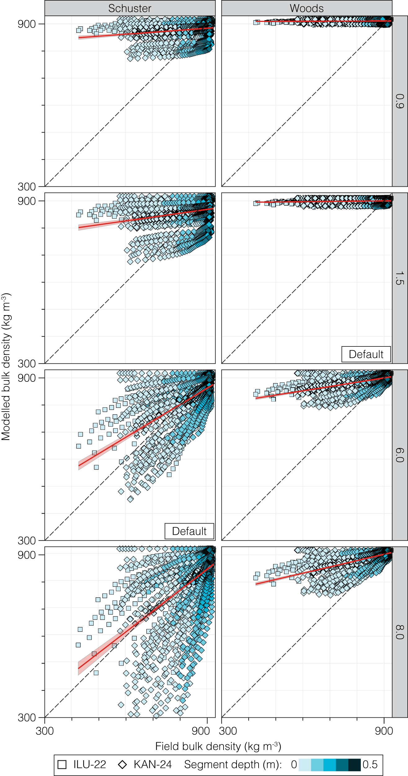
Both models perform poorly when evaluated against field density (Fig. 6). The Schuster model typically underestimates ice density when field measured density is above 800 kg m⁻³, and overestimates density below this threshold. There is no systematic relationship between under/over prediction of density and core segment depth or field site (Fig. 6). This is due to the Schuster model generating a greater degree of weathering deep within the ice column than is observed in the field data and vice versa. The Woods model underestimates the degree of weathering in all model runs (Fig. 6), producing shallow weathering crusts with higher bulk ice densities than either the field measurements or Schuster model (Figs. 3–5). This behaviour corresponds with Woods and Hewitt’s (Reference Woods and Hewitt2024) own reporting of their model (see figure 9 in Woods and Hewitt, Reference Woods and Hewitt2024, p. 17) when using seasonal-like sinusoidal forcings of SWR, LWR and turbulent fluxes.

Figure 6.

Modelled bulk ice density c.f. Field measured bulk density for each of the two models. Regression coefficients are shown in Table 1. The dashed line indicates a ‘perfect density estimate’ (i.e. field measured density equal to modelled density). Segment depth (0.1 m bins) is indicated using colour, while core location is indicated by point shape. There is no systematic relationship between under/over prediction of density and core segment depth or field site. A linear model fit is presented in red, to assist with the comparative visualisation of the data to the dashed line of 1:1 modelled-field density ratio (n = 1831).

Second, we evaluate the ability of the models to capture the growth-decay-growth evolution pattern observed in the field experiments. Both models capture the initial weathering crust growth phase, but neither model fully captures the overnight decay phase (c.f. Figs. 3–5). The two models exhibit differing behaviour during the night: the Schuster model exhibits ongoing weathering crust growth, albeit at a reduced rate compared to the growth phase, while the Woods model exhibits either a bottom-up or top-down density increase driven by refreezing. The ‘regrowth’ phase observed in the field data is only observed in the Woods model for WCR1 and WCR 2.

5.2. Exploration of model performance

5.2.1. Individual core segment density prediction

One explanation for the difference between modelled and field density is that modelled energy distribution across the depth profile poorly reflects the real-world weathering process. This process is represented in the models by the extinction coefficient, which defines the absorption, scattering and therefore energy flux from SWR through the ice column. The Schuster model uses an extinction coefficient of 6 m⁻¹, and the Woods model an extinction coefficient of 1.5 m⁻¹. One potential avenue to improve the alignment between the model output and field data is to use a different extinction coefficient. We completed supplementary model runs using extinction coefficients of 0.9, 1.5, 6.0 and 8.0 m⁻¹ (after Cooper and others Reference Cooper2021). These supplementary runs produced outputs as expected, with higher extinction coefficients generating weathering crusts with lower densities and shallower depths than those which used lower extinction coefficients (Supplementary Figures S3A, S3B and S4). We assess the goodness-of-fit of the modelled ice density using linear regression and RMSE, using the criteria of: gradient (m) closest to 1, intercept (c) closest to 0, highest r ² and lowest RMSE (Table 2). For the Schuster model, the default extinction coefficient (6.0 m⁻¹) yields the second best linear model fit but exhibits the lowest RMSE. Using an extinction coefficient of 8.0 m⁻¹ generates a closer linear model fit, but a high RMSE implies a lack of suitability and further implies that tuning a static coefficient is unlikely to yield an optimal model output. For the Woods model, the best fit (based on the linear model and RMSE) is found with an extinction coefficient of 8.0 m⁻¹, but this still results in severe underestimation of weathering (Fig. 6). Accordingly, we do not attempt to tune a single constant value for this poorly understood variable, especially without a physical dataset to do so, rather these model outputs represent the parameter space and highlight the sensitivity of these models to the choice of extinction coefficient. The use of a single broadband extinction coefficient may not be appropriate due to the way glacier ice absorbs and scatters light, and the dynamic nature of an actively evolving weathering crust. Several studies (Warren, Reference Warren1984; Warren and others Reference Warren, Brandt and Grenfell2006; Cooper and others Reference Cooper2021) highlight the wavelength-variable absorption and transmission of light through glacier ice, implying differential maximum penetration depths for light of different wavelengths. Furthermore, the specific surface area (SSA) of the ice (a measure capturing the surface of scattering interfaces per unit mass) changes as the weathering crust evolves, implying that the extinction coefficient also changes temporally. One future avenue to establish such a dynamic extinction coefficient, that corresponds more closely to real world conditions, would be to couple a weathering crust evolution model with a radiative transfer model that calculates depth-variable extinction coefficients accounting for spatiotemporally variable SSA.

Table 2.

Regression coefficients and RMSE for each extinction coefficient.

* Notes: Default coefficients are indicated as such (*).

The Woods model appears to underestimate ice melt rates and overestimates the role of meltwater refreezing than is observed in the field, resulting in overestimation of ice density. As meltwater is not considered in the Schuster model (Table 1), the following analysis is relevant only to the Woods model. In addition to consideration of the extinction coefficient, the Woods model also requires further hydrological development to reach its full potential (although we note a framework for this can be found in Woods, Reference Woods2024, where water flux is explicitly modelled). For example, such development could include the addition of an active water table, which is observed in the weathering crust (Cook and others Reference Cook, Hodson and Irvine-Fynn2015; Stevens and others Reference Stevens2018). This goal could be achieved using estimates of weathering crust hydraulic conductivity and throughflow (Stevens and others Reference Stevens2018; Irvine-Fynn and others Reference Irvine-Fynn2021; Doting and others Reference Doting2025) to prescribe drainage values or by building empirical relationships between ice density and critical hydrological variables such as effective porosity (e.g. Cooper and others Reference Cooper2018; Halbach and others Reference Halbach2023). We hypothesise such development would lessen the refreeze-effect and more accurately resemble the real-world setting where the water table in the weathering crust is >0.1 m below the surface (e.g. Stevens and others Reference Stevens2018).

5.2.2. Replication of the growth-decay-regrowth evolution pattern

All model runs replicate the initial growth phase of the weathering crust (Figs. 4 and 5), as observed in the field (Fig. 3), driven by high SWR receipt during the day. The Schuster model does not replicate the decay phase observed in the field data. The model functions by calculating the relative rates of surface lowering with internal mass loss, by partitioning energy across the depth profile (Table 1), and weathering crust decay occurs when the rate of surface lowering exceeds the rate of internal mass loss. To reproduce weathering crust decay, the Schuster model requires high turbulent energy flux and low SWR flux, but these conditions do not appear to occur in our meteorological measurement window. The model’s lack of capability to consider meltwater refreezing appears to limit its ability to reproduce the observed decay phase.

For the S15 experiment, the Woods model also does not reproduce the decay phase, and consequently neither a regrowth phase (Fig. 5, Supplementary Figure S1). Rather, it behaves much like the Schuster model (Fig. 4) with a slowdown in weathering overnight in the upper 450 mm of the core profile. However, the model produces a degree of ‘bottom-up’ refreezing (Fig. 5 and Supplementary Figure S1). Refreezing is not observed at the surface during this experiment, where air temperatures exceed 2°C during the decay phase (Fig. 2), ensuring the ice temperatures in the upper ∼500 mm of the core remain above 0°C. Rather a reduction in SWR receipt overnight (Fig. 2) combined with sub-zero ice temperatures at depths >0.5 m (Supplementary Figure S2) drives bottom-up refreezing. This is not observed in the field data (Fig. 3) which only exhibits a density increase from 426 to 762 kg m⁻³ in the upper ∼300 mm of the core during the overnight decay phase, and no refreezing below 0.45 m. All four KAN-24 experiments (WCR1–4) exhibit a decay phase in the Woods model output (Fig. 5, Supplementary Figure S1), where the weathering crust freezes from the top down overnight. This process occurs between midnight, when SWR receipt is reduced to ∼0 W m⁻² and air temperature falls, and 9 AM for WCRs 1 and 2. For WCRs 3 and 4, air temperatures are several degrees lower than for WCRs 1 and 2 (Fig. 2), falling as low as −4°C, and consequently the freezing front penetrates further into the weathering crust to a depth of 0.19 m (c.f. to 0.1 mm for WCRs 1 and 2). This top-down freezing front is not observed in the field data.

The regrowth phase, observed at all KAN-24 sites in the field (but not the S15 experiment at ILU-22, which was curtailed due to the onset of rain at 0845) is only reproduced by the Woods model runs at WCR 1 and 2, and not in the WCR3 and 4 model runs. However, both the Schuster model (all model runs) and Woods model at S15 exhibit an acceleration in weathering (c.f. the overnight rate decrease in weathering) during the period the regrowth phase is observed in the field data. In the Woods model runs, no regrowth phase is observed at WCRs 3 and 4, where the ice temperature remains below freezing to the end of the 25 hour model run at ∼1100 (Supplementary Figure S2). In contrast, WCRs 1 and 2 see a return to ice temperatures at 0°C, causing weathering both above and below the freezing front, maintaining the stepped density profile created during the decay phase (Fig. 5). The likely driver of this difference in behaviour is air temperature, which is 1°C at WCRs 1 and 2 during the regrowth period, but −1°C at WCRs 3 and 4. As such, we assert the differing behaviour of the Woods model between different sets of environmental conditions can be explained by the conditions themselves.

The differing behaviour of the two models during the decay phase can be explained by the assumptions each model is based upon, as summarised in Table 1. When considered alongside the field data, such behaviour further reinforces the assertion that density increase in the decay phase is driven by multiple processes, some of which are not replicated within the models in their current form. If density increase during the decay phase was driven solely by energy balance and the relationship between the relative rates surface lowering and internal melting, then it would be expected to be captured in the Schuster model—which does not simulate any mass accretion processes (it does not explicitly model ice temperature and simulates the internal removal of mass as the creation of empty pore space, rather than as a phase change from ice to liquid meltwater which can freeze and drive mass accretion). However, the decay process is not captured by this model—implying the existence of additional processes.

In contrast, the Woods model explicitly models ice temperature and assumes that the pore space is occupied by meltwater, which can refreeze. Despite this capability, the Woods model also does not replicate the way the decay phase presents in the field data, where the density increase in the decay phase is observed throughout the depth profile. The Woods model is unable to capture density increase throughout the depth profile because the model assumes local thermal equilibrium (i.e. when both ice and water are present in a region both the ice and water are at the melting temperature). Consequently, freezing can only occur at a freezing ‘front’, as observed in Fig. 5. Moreover, this approach presumes that water is available to refreeze—which, for a surface-down freezing front to reach unweathered bulk ice density (as it does in Fig. 5), requires a fully saturated weathering crust, which is unlikely to be present in the environment as is discussed in Section 4. In the case of a partially saturated crust containing only crystal-bound meltwater, density increase would be limited by water availability, and it would not be possible to reach unweathered bulk ice density. Consequently, we suggest further investigation with (a) field measurements of water table and (b) a model formulation which accounts for non-equilibrium thermodynamics (e.g. Moure and others Reference Moure, Jones, Pawlak, Meyer and Fu2023) and allows for drainage and a fluctuating water table (e.g. Woods, Reference Woods2024) may enhance the capability of this model to replicate the field observations herein.

6. The contribution of ice weathering to broadband albedo

Broadband albedo was measured prior to core extraction at each site between the hours of 1000–1800 (i.e. solar noon ± ∼5 hours), generating 48 individual measurements of broadband albedo from our experimental surfaces. We report different broadband bare ice albedo at each of our study locations: for ILU-22, we observed albedo between 0.52 and 0.58, and for KAN-24 albedo was between 0.38 and 0.45. Both ranges correspond with the reference values for ‘clean-ice’ albedo (Cuffey and Paterson, Reference Cuffey and Paterson2010), and our ILU-22 albedos fall within the observed range for ‘clean’ ice at other sites on the Greenland ice sheet (Wehrlé and others Reference Wehrlé, Box, Niwano, Anesio and Fausto2021). We attribute the difference in albedo between the two sites to three causes: potentially different ice micro-structures (e.g. crystal fabrics, orientation and bubble content, see Jennings and Hambrey, Reference Jennings and Hambrey2021), the use of different instrumentation and the possibility of greater particulate loading at KAN-24 than at ILU-22. For the ILU-22 campaign (the S15 experiment), surface reflectance was measured over a well-defined footprint, using a 10° field of view. In contrast, albedo was measured using a semi-hemispheric Kipp and Zonen CNR4 at KAN-24 (150° field of view), potentially incorporating interference from non-ice reflectors. Furthermore, despite cleaning of the experimental surface, it was not possible to remove particulates from within the ice column—despite the underlying assumption that it was ‘clean’—and this inherent ‘darkness’ may also contribute to lower albedo observations for the KAN-24 sites. Here, outcropping of Late Holocene dust has been reported (Wientjes and others Reference Wientjes, Van De Wal, Schwikowski, Zapf, Fahrni and Wacker2012), and the area around the S6 weather station is renowned for its typically lower-than-average albedo (e.g. Greuell, Reference Greuell2000; van den Broeke and others Reference van den Broeke, Smeets, Ettema and Munneke2008; Feng and others Reference Feng, Cook, Anesio, Benning and Tranter2023).

Our data reveal that bulk ice density of the uppermost 0.1 m of the weathering crust exerts a strong control on bare ice albedo (Fig. 7). The average ice density of this upper section of the weathering crust describes 88–96% of the variation in bare ice broadband albedo throughout our experiment—which we caution was undertaken on an LAP-free, modified surface, rather than a surface in its natural state, and that we do not consider water ponding on the surface. The effect of ice weathering as an albedo driver is further supported by the variations in spectral albedo, which primarily occurred in the near-infrared region (Supplementary Figure S5) where the physical properties of ice are the main control (Gardner and Sharp, Reference Gardner and Sharp2010; Whicker and others Reference Whicker, Flanner, Dang, Zender, Cook and Gardner2022). The relationship between density and broadband albedo was also observed by Dadic and others (Reference Dadic, Mullen, Schneebeli, Brandt and Warren2013) in a blue-ice zone on the East Antarctic Ice Sheet, who considered density as a proxy for SSA. However, they reported a nonlinear relationship (Fig. 7), in contrast to the linear relationship we observe at our field sites. Moreover, they observed much high albedos than our study (up to 0.77 for a density of 500 kg m⁻³, in contrast to the maximum of 0.58 reported herein). We attribute this to differences between the datasets: our data focus on weathered ice, while the Dadic study also includes firn and snow, which typically have higher albedo than bare ice (Cuffey and Patterson, Reference Cuffey and Paterson2010) due to structural differences.

Figure 7.

Bare ice albedo as a function of bulk density of the uppermost 0.1 m of the ice column. Shape and colour are used to differentiate field locations and the logarithmic regression reported by Dadic and others (Reference Dadic, Mullen, Schneebeli, Brandt and Warren2013). Adjusted r ² is presented per location to describe the linear model fit, within the measurement bounds.

We attribute the governing role of near-surface ice density over broadband bare ice albedo to structural changes in the ice crystal matrix associated with weathering, which increases internal scattering. Ice is poorly absorbing in the spectral domain corresponding to SWR (Warren, Reference Warren2019) and consequently the extinction of light within and from the ice column is primarily controlled by the amount of scattering. Scattering is primarily governed by the SSA of polycrystalline ice (Gardner and Sharp, Reference Gardner and Sharp2010), which describes the per-mass surface of air-ice interface area (i.e. the surface area of ice crystals in a given mass of ice) where scattering events occur. SSA is governed by effective grain and pore (also referred to ‘bubble’) size. A dense ice column with few large bubbles has a low SSA and high SWR penetration depth, while a porous column with small air inclusions has a high SSA. The formation of the weathering crust is, to a degree, a negative-feedback process, in which weathering increases porosity and consequently SSA, causing more scattering, increasing broadband surface albedo and reducing depth penetration of SWR (Dadic and others Reference Dadic, Mullen, Schneebeli, Brandt and Warren2013; Garzonio and others Reference Garzonio2018). This feedback is further complicated by the presence of water within the weathering crust, which can fill pore spaces and reduce SSA, scatter and albedo. The uppermost 0.1 m of the weathering crust (as examined in this analysis) is generally unsaturated Stevens (and Stevens and others Reference Stevens2018; Reference Stevens2019; see Section 4), although water table measurements were not directly measured during this study. Hence, the role of water is not considered herein, especially considering the lack of field data—but the role of interstitial meltwater should not be disregarded in the cases where the water table is within 0.1 m of the ice surface.

For the range of ice densities measured herein, our data demonstrate that ice condition can drive a maximum albedo change of 0.05. However, it is unclear whether our experimental surfaces reach equilibrium with a fully developed weathering crust (discussed in further detail in Section 4), and as such this value is unlikely to represent the fully range of density-controlled albedo. By extrapolating the linear relationships identified in Fig. 7, using the lowest quoted value for weathering crust density for the uppermost 0.1 m (300 kg m⁻³; LaChapelle, Reference LaChapelle1959; Cooper and others Reference Cooper2018) we imply that near surface ice density has the potential to increase albedo by 0.09 c.f. unweathered ice. Using our field-derived albedo changes driven by the process of weathering, we calculate that the formation of weathering crust has a mean radiative forcing effect of −11.2 W m⁻² (range of −8.0 to −14.2 W m⁻²; n = 5) during our study periods. Taking the maximum potential albedo increase due to weathering or 0.09, we suggest that radiative forcing due to near-surface ice weathering may reach up to −24.3 W m⁻² (range −22.9 to −26.7 W m⁻²; n = 3). This is less than the weathering-driven albedo increase of 0.15 observed on Antarctic ice shelves by Traversa and Di Mauro (Reference Traversa and Di Mauro2024), equivalent to a radiative forcing of −85 W m². The maximum radiative forcing due to ice weathering we suggest is lower than Traversa and Di Mauro (Reference Traversa and Di Mauro2024) for two reasons: we report a lower albedo differential between unweathered and weathered surfaces (due to the high albedo of blue ice areas—commonly 0.50–0.70 for unweathered blue ice, with weathered ice reaching 0.78—compared to unweathered ice on the Greenland ice sheet); and SWR receipt for our experimental periods is generally lower than in the high Austral summer. Note that by applying Traversa and Di Mauro (Reference Traversa and Di Mauro2024) albedo change to our meteorological conditions would cause a mean radiative forcing of −40.7 W m⁻² (range −37.5 to −44.5 W m⁻²; n = 3).

We demonstrate that, for ‘clean’ ice (i.e. a surface with minimal LAPs), the condition of the weathering crust has the potential to increase albedo by 0.09, in contrast to the well-documented albedo-reducing effects of both abiotic and biotic LAPs (Ryan and others Reference Ryan2018; Chevrollier and others Reference Chevrollier2022). While it is possible to draw simplistic numerical comparisons with reported albedo reduction effects of LAPs, it is important to consider the interplay between the presence of LAPs and ice weathering. When LAPs are present, they absorb SWR (Warren, Reference Warren2019)—reducing the energy receipt within the near-surface ice which forms the weathering crust. Through this mechanism, LAP presence reduces the intensity of ice weathering, and as such in areas with high LAP loading (e.g. the Dark Zone), the weathering crust is unlikely to reach its full potential for albedo change. Therefore, it is somewhat complex to evaluate the relative roles of the weathering crust and LAPs on albedo, and any such analysis should be considered with a degree of caution.

Ryan and others (Reference Ryan2018) report an albedo differential of 0.28 between ‘predominantly clean ice’ and ‘ice containing uniformly distributed impurities’ (0.55 and 0.27, respectively), on a transect which includes the KAN-24 site, but do not distinguish between the contribution of LAPs and the weathering crust. By correcting extrapolatively for the albedo increase of a fully formed weathering crust, and thereby assuming an unweathered ice albedo of 0.46 (0.55–0.09), we can extrapolate a minimum LAP-driven albedo reduction of 0.19 from Ryan and others (Reference Ryan2018)—and a maximum LAP-derived reduction of 0.28, assuming no weathering crust is present in the ‘predominantly clean ice’ areas. Moreover, Chevrollier and others (Reference Chevrollier2022) report an albedo reduction potential of up to 0.10 (range 0.01–0.10, depending on algal concentration) from glacier algae alone, using algal optical properties and applying a radiative transfer model. The albedo effect of algae appears similar to that of the weathering crust. However, considering that glacier algae is often combined with other LAPs undocumented in this specific study (i.e. mineral dust, black carbon, distributed cryoconite material), and the work of Ryan and others (Reference Ryan2018), we suggest that the albedo-modifying effect of the weathering crust may be secondary to that of LAPs at a point scale. We caveat this statement heavily however, due to the large uncertainties, assumptions and lack of direct data—rather highlighting an additional complexity when considering albedo-modification processes on the Greenland ice sheet and the remaining lack of understanding about the interplay between weathering crust condition, LAP concentrations and albedo.

The relative roles of each albedo-modifying component considered here (i.e. weathering crust condition and LAP effects) vary in space across the ablation zone of the Greenland ice sheet. For example, Ryan and others (Reference Ryan2018) highlight ‘clean’, LAP-‘free’ areas on the K-Transect, both above and below the so-called ‘Dark Zone’. In these ‘clean’ ice areas, the condition of the weathering crust is likely to be the primary driver of sub-seasonal albedo fluctuations, as was highlighted by Tedstone and others (Reference Tedstone2020). Ultimately, the physical condition of near-surface ice plays a role in defining broadband surface albedo, and further work should focus on the interplay between ice condition and LAPs and their roles in albedo moderation.

7. Summary

We present a method to ‘reset’ the near-surface weathering crust and measure its development, designed for explorations of its evolution. Our 383 measurements on the Greenland ice sheet reveal ice densities from 420 kg m⁻³ to 920 kg m⁻³, providing the largest study of weathering crust condition to date. We observe the hypothesised nonlinear depth–density relationship, a result of the nonlinear receipt of SWR throughout the ice column. However, we typically observe shallower weathering crusts than previous work has reported: we report depths of up to 0.5 m, while others report depths up to 2 m—albeit in different locations to those in this study, which may subsequently be associated with differing energy balance (namely, a relatively lower proportional turbulent flux receipt).

We reveal diurnal switching behaviour in the process of weathering crust evolution. During the day, under clear sky conditions (i.e. high SWR receipt), the near-surface of the ice is actively—and potentially rapidly—weathering. An LAP-free, unweathered ice surface evolves quickly, with the uppermost ∼0.05 m of the ice column weathering at rates of up to −80 kg m⁻³ h⁻¹. During periods of low SWR receipt (in this case, overnight—but this could also occur under cloudy conditions) weathering rate reduces, and the density of the weathering crust effectively increases. We suggest that a combination of surface lowering, refreezing of interstitial meltwater and hoar deposition drive this process. We suggest future studies should seek to monitor the position of the water table, measure ice temperature and examine ice crystallography, enabling a more in-depth exploration of the processes driving weathering crust decay. Density reduction resumes following a return to ‘high’ SWR conditions. This rapid rate of change of near-surface ice density has implications for supraglacial hydrology: the weathering crust demonstrates the potential to change on an hourly timescale, which will affect its effective porosity and meltwater transmissivity. Ice density in the upper 0.1 m of the ice column demonstrates a negative relationship with bare ice albedo: weathered ice is more reflective than unweathered ice. The magnitude of this effect is important, with potential to cause a radiative forcing change of −24.3 W m^−2, but it is likely that the albedo-modifying effect of the weathering crust is secondary to the competing role of LAPs at our study sites.

Two numerical models describing weathering crust formation (Schuster, Reference Schuster2001; Woods and Hewitt, Reference Woods and Hewitt2023, Reference Woods and Hewitt2024) were evaluated against our field measurements. Neither model reliably recreates the field observations. The Woods model produced weathering crusts with higher densities than observed in the field (i.e. minimum density >870 kg m⁻³), while the Schuster model failed to capture the overnight decay phase of the weathering crust, and underestimated weathering when field measurements of ice density are less than 800 kg m⁻³. Ultimately, our field observations and model evaluation reveal that we still have a poor mechanistic understanding of near-surface ice weathering, most notably the partitioning of energy between the ice surface and near-surface, and the absorption/extinction/reflection of light through a column of polycrystalline ice.