


Introduction
The McMurdo Dry Valleys comprise the largest ice-free region in Antarctica, and they represent a globally unique cold desert environment containing unique biological (Lee et al. Reference Lee, Laughlin, Bottos, Caruso, Joy and Barrett2019, Collins et al. Reference Collins, Young, Convey, Chown, Cary and Adams2023) and geological (Levy et al. Reference Levy, Fountain, Dickson, Head, Okal, Marchant and Watters2013) features. For example, vascular plants and vertebrates are absent, and the macroscopic biota consists largely of invertebrates such as Collembola (springtails) and mites, as well as mosses and lichen (Adams et al. Reference Adams, Bardgett, Ayres, Wall, Aislabie and Bamforth2006). They are also sensitive to atmospheric changes such as global warming (Hogg & Wall Reference Hogg and Wall2011). Increases in atmospheric temperatures are expected to lead to substantial glacier melt (Kennedy Reference Kennedy1995, Lee et al. Reference Lee, Waterman, Shaw, Bergstrom, Lynch, Wall and Robinson2022a), resulting in increased soil moisture (Wall Reference Wall2007). This will produce more ice-free areas capable of supporting the resident biota (Smith et al. Reference Smith, Wall, Hogg, Adams, Nielsen and Virginia2012, Lee et al. Reference Lee, Raymond, Bracegirdle, Chades, Fuller, Shaw and Terauds2017), as well as providing suitable habitat for invasive species (Chown et al. Reference Chown, Huiskes, Gremmen, Lee, Terauds and Crosbie2012, Duffy & Lee Reference Duffy and Lee2019, Lee et al. Reference Lee, Terauds, Carwardine, Shaw, Fuller and Possingham2022b). The Dry Valleys are therefore likely to see dramatic changes as the availability of liquid water limits biotic activity in terrestrial Antarctica (Kennedy Reference Kennedy1993, Cary et al. Reference Cary, McDonald, Barrett and Cowan2010). The magnitude of the anticipated environmental changes on Antarctica’s unique and sensitive ice-free regions requires careful and ongoing attention (Gutt et al. Reference Gutt, Isla, Xavier, Adams, Ahn and Cheng2021).
Modelling the spatial distribution of biota in the Dry Valleys would help us to understand the potential consequences of climate change. The process of accurately predicting the distribution of biota will help build scientific knowledge regarding the spatial drivers for the resident biota. The isolation and extreme cold temperatures in the Dry Valleys mean that only a few species exist in this region, removing the complexity of interspecific competition common within most other ecosystems (Hogg et al. Reference Hogg, Cary, Convey, Newsham, O’Donnell and Adams2006). In essence, modelling the distribution of biota in the Dry Valleys using fundamental physical (abiotic) drivers provides a test of spatial modelling for predicting biotic distribution in more complex habitats elsewhere.
The extreme dry and cold environment of the Dry Valleys means that access to liquid water is a critical driver of biota alongside temperature (Green et al. Reference Green, Sancho, Pintado and Schroeter2011, Hogg & Wall Reference Hogg, Wall and Bell2012). The latter is important for biotic activity and also determines the rate at which snow and ice melt, resulting in liquid water being potentially available to the biota (Gooseff et al. Reference Gooseff, Barrett, Doran, Fountain, Lyons, Parsons and Wall2003). Another critical element of habitat suitability is a stable environment that is free from rock movement or windblown gravel and sand (Lee et al. Reference Lee, Laughlin, Bottos, Caruso, Joy and Barrett2019). Essentially, very few physical factors can determine suitable habitat for biota. Suitable habitats are likely to include sheltered locations with sunny, warm northerly aspects with access to meltwater from glaciers or large snow patches. Lichen habitats are the exception, which essentially require stable rock where moisture is derived from water vapour (Green et al. Reference Green, Sancho, Pintado and Schroeter2011).
Biotic systems in the Dry Valleys are relatively simple and are thought to be primarily influenced by abiotic factors (Gooseff et al. Reference Gooseff, Barrett, Doran, Fountain, Lyons, Parsons and Wall2003, Hogg et al. Reference Hogg, Cary, Convey, Newsham, O’Donnell and Adams2006), although some biotic interactions are probable (Caruso et al. Reference Caruso, Hogg, Nielsen, Bottos, Lee and Hopkins2019, Lee et al. Reference Lee, Laughlin, Bottos, Caruso, Joy and Barrett2019). However, we still lack models of biota at scales relevant to the actual organisms (Caruso et al. Reference Caruso, Hogg, Carapelli, Frati and Bargagli2009). This knowledge gap persists, even with the abundance of abiotic data that could be used for predicting the distribution of biota in Antarctica. For example, although polar-orbiting satellites such as Landsat 8/9 have a nominal revisit frequency of 16 days, high-latitude swath overlap means that parts of Antarctica may be imaged more frequently. This increased frequency makes satellite data particularly useful for monitoring Antarctica.
Predictive spatial modelling, which has developed rapidly in recent years with cloud-based supercomputers, machine learning and explainable artificial intelligence (AI), may be particularly helpful in this regard (Arrieta et al. Reference Arrieta, Díaz-Rodríguez, Del Ser, Bennetot, Tabik and Barbado2020, Linardatos et al. Reference Linardatos, Papastefanopoulos and Kotsiantis2021). These advances have facilitated access to big data and data-mining techniques, allowing more detailed analyses and spatial characterization of natural ecosystems (De Reu et al. Reference De Reu, Bourgeois, Bats, Zwertvaegher, Gelorini and De Smedt2013, Castle et al. Reference Castle, Hebert, Clare, Hogg and Tremblay2021).
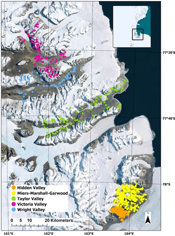
Here, we use an existing and comprehensive dataset from the New Zealand Terrestrial Antarctic Biocomplexity Survey (NZTABS; Caruso et al. Reference Caruso, Hogg, Nielsen, Bottos, Lee and Hopkins2019, Lee et al. Reference Lee, Laughlin, Bottos, Caruso, Joy and Barrett2019) and assess the potential of these data for spatial modelling of terrestrial biota across the whole of the McMurdo Dry Valleys. We then combine these data with a wetness model (Stichbury et al. Reference Stichbury, Brabyn, Green and Cary2011), based on glacier surface melt rates and water routing models (Brabyn & Stichbury Reference Brabyn and Stichbury2020). Prior modelling analyses using the NZTABS data have been mostly restricted to the southern Dry Valleys (Miers, Marshall and Garwood valleys; see Caruso et al. Reference Caruso, Hogg, Nielsen, Bottos, Lee and Hopkins2019, Lee et al. Reference Lee, Laughlin, Bottos, Caruso, Joy and Barrett2019, Bottos et al. Reference Bottos, Laughlin, Herbold, Lee, McDonald and Cary2020). These southern valleys represent a small portion of the overall Dry Valleys and of the total area surveyed as part of NZTABS. Here, we expand on this previous coverage to also include the much larger Taylor, Wright and Victoria valleys (Fig. 1).
Location of the study area in the Ross Sea region of Antarctic (inset map) and the survey points used in the New Zealand Terrestrial Antarctic Biocomplexity Survey (NZTABS) study. The different valleys surveyed are represented by different colours, as indicated in the figure legend.

The main aims of our study were to demonstrate the use of GIS and satellite-derived variables, including elevation, temperature and moisture, to predict the spatial distribution of Antarctic biota and to facilitate further understanding of the environmental drivers of biota in the McMurdo Dry Valleys.
Materials and methods
Data provenance and study area
The initial spatial modelling of mosses and lichens in the McMurdo Dry Valleys was conceived in 2002 by Brabyn and Green (unpublished data; Lee et al. 2019). Subsequently, the project grew to include the distribution of soil microbes as well as metazoans (nematodes, mites, springtails) and to involve a range of scientists covering microbiology, botany, zoology, geology, soils and GIS. Together, this group became the International Centre for Terrestrial Antarctic Research (ICTAR; https://ictar.aq/). The resulting research project was NZTABS, with research goals being expanded to focus on the spatial relationship between landscape and the biota and to determine the relative importance of abiotic and biotic drivers of biodiversity.
The NZTABS field data were collected over six field seasons between 2009 and 2014 covering much of the Dry Valleys (Fig. 1).
Metadata for NZTABS have been archived and were obtained from the following sites: https://www.gbif.org/dataset/0821ab21-c6a5-4757-91c2-1f5e95d0ecda#description and https://antcat.antarcticanz.govt.nz/geonetwork/srv/api/records/91a5c352-7930-4541-a238-63ba06131591.
Data availability and model inputs
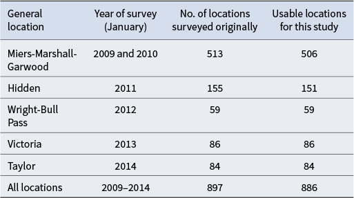
Table I provides a summary of the number of locations surveyed for each of the major valleys visited, as well as the number of records that were usable for the modelling. Some original data records were removed because they were missing essential information such as coordinates or biological survey data.
Summary of the New Zealand Terrestrial Antarctic Biocomplexity Survey (NZTABS) field surveys and the number of recorded locations for each survey as well as the number of locations used for the current study.

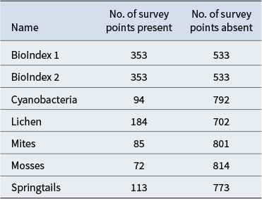
Response variables and the number of survey points where data were present/absent are shown in Table II. There were 533 survey locations where macroscopic biota was absent, 229 locations where one biotic type was present, 73 with two types, 32 with three types, 18 with four types and one with all five biotic elements present. Two biodiversity indices were calculated and also used as response variables: BioIndex 1 was the number of unique biota present (i.e. lichens, mosses, mites, springtails, cyanobacteria, range 0–5), and BioIndex 2 was the presence of any of the five biotic types. The response variables were modelled as a classification and as a regression. The classification used presence/absence (apart from BioIndex 1, which had values from 0 to 5). The regression used percentage cover for cyanobacteria, moss and lichens, 0 or 1 for springtails, mites and BioIndex 2, and 0–5 for BioIndex 1. Even though the survey produced counts of the number of springtails and mites at each site, an accurate and comparable count was considered challenging because of their small size and variable weather conditions at the time of sampling. Accordingly, presence/absence values were perceived as being more reliable.
Response variables used as well as the number of survey points present or absent for each variable.

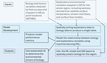
The inputs to the model consist of biotic survey data, which are the response variables, and GIS-derived environmental data (Table III), which are the explanatory or predictor variables. The response and explanatory variables are spatially combined with GIS to produce a single table, and the relationships between these variables were modelled using random forest. Model performance and explainable AI were used to assess and understand this model. This random forest model was also used to spatially predict the biota beyond the locations surveyed using the GIS layers of the explanatory variables. Figure 2 provides an overview of the modelling process, and a more detailed description follows below.
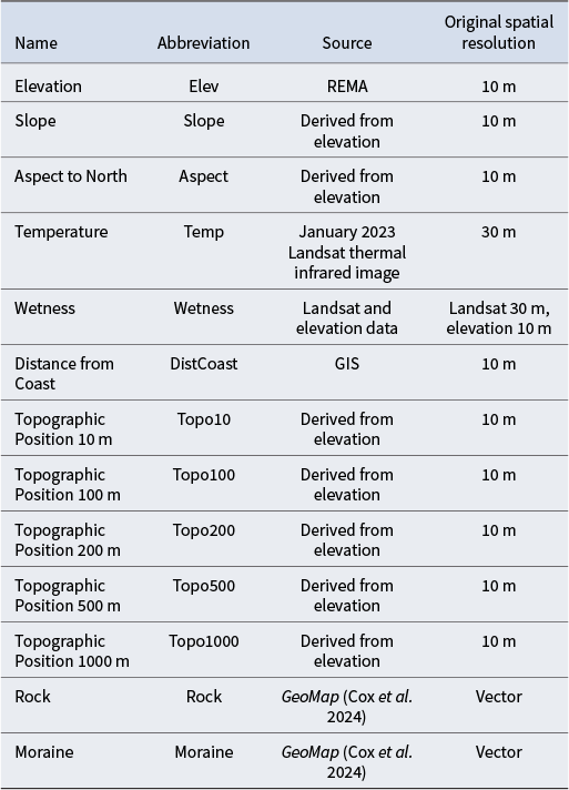
Explanatory variables used for analyses including abbreviations used, data source and original spatial resolution of the data.

REMA = Reference Elevation Model of Antarctica.
Overview of modelling process showing model inputs, model development and outputs of the model. AI = artificial intelligence; NSTABS = New Zealand Terrestrial Antarctic Biocomplexity Survey.

The NZTABS data include GPS locations of the sample points, biotic data (both macro and micro) and GIS-derived topographical information, including wetness. The lichens, cyanobacteria and mosses were quantified using a 20 m × 2 m transit at each location. The extents of cyanobacteria, lichen and moss cover were each measured by walking along the transit with a 1 m pole and counting the number of 100 cm2 units for each taxon. This count was then converted to percentage cover. The survey of springtails and mites was carried out by examining the underside of small (5–10 cm diameter), flat (< 2 cm thickness) and preferably dark rocks within a 20 m radius of the survey location. The numbers of springtails and mites were recorded. The survey locations used a stratified random sampling approach based on elevation, slope, aspect and geology. The accuracy of the GPS locations is ~1–6 m. This accuracy needs to be considered when overlaying with GIS layers.
Explanatory variables
Table III provides a list of explanatory variables and their sources used for the predictive spatial modelling. A more detailed description of these variables follows: the elevation data used were from the Reference Elevation Model of Antarctica (REMA) and were downloaded from the Polar Geospatial Center (https://www.pgc.umn.edu/). The spatial resolution for these data was 10 m (Howat et al. Reference Howat, Porter, Smith, Noh and Morin2019). The higher-resolution LiDAR data available for McMurdo Dry Valleys (Wilson & Csatho Reference Wilson and Csatho2007) were also considered. However, these was deemed unnecessary because the REMA data with 10 m spatial resolution were sufficient, given that they were being used with satellite data that had 30 m resolution. Slope and aspect were calculated from the elevation data using the standard slope and aspect function in GIS. Since aspect is circular (i.e. 359° is close to 1°), the degrees were converted to the distance from north, with the maximum value being 180° (south). Mean temperature was calculated from all the Landsat 8 and Landsat 9 thermal infrared images that were cloud free for the month of January 2024. A total of 49 images were used from the Google Earth Engine Data Catalog (https://developers.google.com/earth-engine/datasets).
The wetness layer was derived from a model based on the relationship between Landsat surface temperatures of glaciers, the size of the glaciers and the estimated meltwater derived at these temperatures from the glaciers using stream discharge data for Taylor and Wright valleys, which are part of the McMurdo Long-Term Ecological Research Program (www.mcmlter.org). The flow path and accumulation of this meltwater were modelled in GIS using elevation data and the Compound Terrain Index (Stichbury et al. Reference Stichbury, Brabyn, Green and Cary2011). A complete explanation of this method is provided by Brabyn & Stichbury (Reference Brabyn and Stichbury2020). As glacier surfaces become warmer, which can be measured from satellites using thermal infrared data, the increased water melt and subsequent water flows and accumulations can be calculated. The wetness index was recalculated using a new melt rate model derived from 21 cloud-free Landsat 8 thermal infrared sensor (TIRS) data-only Tier 2 product (Earth Resources Observation and Science Center 2024 ). These images were captured between 2014 and 2023 during the month of January. The resolution of this band is 100 m, although the data product was resampled to 30 m. In total, 130 data points that linked glacier surface temperatures and melt discharge were used, generating an ordinary least squares (OLS) regression (r 2 = 0.80). The flow direction, accumulation and final wetness index were derived using the 10 m REMA elevation data described previously.
Distance from coast was calculated using the Euclidean Distance in ArcPro and the high-resolution Antarctic coastline layer obtained from the Scientific Committee on Antarctic Research (SCAR) Antarctic Digital Database (https://scar.org/library-data/maps/add-digital-database). The Topographic Position layers are measures of the relative elevation of a location in relation to the highest and lowest points in the surrounding region (Wilson & Gallant Reference Wilson and Gallant2000, De Reu et al. Reference De Reu, Bourgeois, Bats, Zwertvaegher, Gelorini and De Smedt2013). This measure indicates whether the location is at the highest point, such as a ridge top, or the lowest point, such as a valley floor, or somewhere in-between. Ridges or valley floors experience a range of different environmental conditions, including climate variables and water availability, as well as different geomorphological processes, such as erosion and deposition. Ridge tops can often consist of stable substrate, such as bedrock, while valley floors may have loose substrate, such as sand and gravel. Topographical Position can exist at different scales, from mountain ridges and valleys to small mounds and indentations. This research uses a range of scales to determine which scale is relevant. The Topographic Position is the elevation of a pixel minus the mean elevation of the surrounding pixels in a defined area. The extent of the surrounding area determines the scale of the calculation. For this research, a sequence of surrounding regions was used, ranging from a radius of 10 to 1000 m (see Table I).
The Moraine and Rock variables were derived from GeoMap (Cox et al. Reference Cox, Smith Lyttle, Elkind, Siddoway, Morin and Capponi2023) using the ‘POLYGTYPE’ field and were represented as 0 (absent) and 1 (present). The purpose of these explanatory variables was to represent the stability of the surface. Moraine is mostly loose, unconsolidated substrate that can be transported by wind, making it difficult for most biota to establish upon. Although these variables were based on presence or absence, they were treated as numerical values, as modelling using categorical classes produces separate models and data for each class.
Spatial predictive modelling using Random Forest
To examine the NZTABS data, we used the Random Forest machine learning tool (Breiman Reference Breiman2001) in combination with the explainable AI tool SHapley Additive exPlanations (SHAP) graphs (Lundberg & Lee Reference Lundberg, Lee, von Luxburg, Guyon, Bengio, Wallach and Fergus2017) to interpret the main drivers of biota in the Dry Valleys. Random Forest is a decision tree algorithm that resolves many of the instability problems with OLS regression models (Cutler et al. Reference Cutler, Edwards, Beard, Cutler, Hess, Gibson and Lawler2007). One criticism of machine learning is that it is a ‘black box’ approach, and although it produces high predictive performance, it provides poorer explanatory data compared with traditional OLS regressions, which provide coefficient values for each explanatory variable. Explainable AI (Arrieta et al. Reference Arrieta, Díaz-Rodríguez, Del Ser, Bennetot, Tabik and Barbado2020, Linardatos et al. Reference Linardatos, Papastefanopoulos and Kotsiantis2021) addresses this criticism, with SHAP graphs providing a potential solution. Specifically, SHAP graphs show the importance of each explanatory variable and the direction of influence (positive or negative), providing similar information to the coefficient values from OLS regressions.
Initially, the ArcPro ‘Predict using Regression Model’ tool was used, which is in the arcpy library and includes a prediction map as an output. Unfortunately, this prediction model in ArcPro could not be integrated with SHAP graphs. Instead, RStudio (version 4.4.2) was used because it could combine Random Forest (version 4.7-1.2) and SHAP graphs (shapeviz version 0.10.2). Although other data-boosting algorithms (used to improve models) were available, such as CatBoost (Prokhorenkova et al. Reference Prokhorenkova, Gusev, Vorobev, Dorogush and Gulin2019), Random Forest was chosen because it is widely used in ecological predictions (see Pham & Brabyn Reference Pham and Brabyn2017).
With Random Forest, several parameters are fine-tuned to maximize the performance of the model (Li et al. Reference Li, Justy, Siwabessy, Tran, Huang, Heap, Zhao and Cen2014). An important parameter is the percentage of the data used for training the model and the percentage used for validation (Rodriguez-Galiano et al. Reference Rodriguez-Galiano, Ghimire, Rogan, Chica-Olmo and Rigol-Sanchez2012). Experiments were conducted using a range of data splits, resulting in the best split being Training 75% and Validation 25%. The Ntree parameter had the best average performance using the value 500. The Mtry parameter was optimized for each model using the caret package (version 7.0-1). The kappa statistic and percentage of variation explained were used for reporting the performance of the classification and regression models, respectively. As the number of data points was relatively low in relation to the complexity and diversity of the data, the data points used for the training and validation can affect the model and the performance of the model. Accordingly, the data splitting was based on a random process determined by a seed value. Similar seed values mean that the data split is similar. Changing the seed values leads to the data split being different, resulting in the model and performance metrics also being different. For this reason, the caret package was used to rerun the model 100 times using different seed values and the average model performance was calculated. The explainable AI and prediction maps used the seed value of 151.
Results
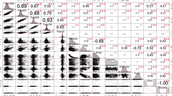
Figure 3 shows correlation values among variables, scatter plots and data distribution plots for each of the explanatory variables used to assess the distribution of biota in the Dry Valleys. Higher elevations tend to have steeper slopes, lower temperatures and can be drier due to increased runoff of water vs water accumulation at lower elevations. This is reflected in the strong, significant, negative correlations between slope and wetness (R 2 = −0.88, P < 0.01; Fig. 3). The weaker but still significant correlation values between aspect and slope (R 2 = −0.18, P < 0.01) can also be explained by the general direction of the valleys, which are typically east to west, resulting in the valley walls having north or south aspects. The Topographic Position indices that had similar scales (e.g. Topo1000 and Topo500 or Topo10 and Topo100) were strongly correlated (R 2 > 0.65, P < 0.01 in all cases). In contrast, the scales that differed (e.g. Topo1000 and Topo10) showed weaker correlation (R 2 = 0.21). The distribution of the data for each of the variables is shown along on the main central diagonal of Fig. 3. For Aspect, the data were evenly distributed, as this variable was deliberately stratified as part of the sampling strategy for NZTABS. Data distributions for other variables reflect the distribution of the topography that was accessible in the study area. For example, as most of the study area was relatively dry, and because wetness values were not stratified as part of the sampling strategy, only a limited number of wet areas were ultimately sampled (e.g. see Wetness frame, Fig. 3).
Correlation matrix and data distribution for variables shown along the diagonal of the matrix. Abbreviations for variables correspond to those listed in Table III. The sampling data and distributions for each of the variables used as part of the modelling are named and shown along the diagonal of the figure. Above the diagonal shows the correlation matrix, with the magnitude of the correlation (R values) reflected by font size: larger fonts indicate stronger correlations (both positive and negative). The level of significance for the correlations is represented by the number of asterisks: * P < 0.1, ** P < 0.05, *** P < 0.01. Below the diagonal are the individual scatter plots and/or data distribution plots (red lines).

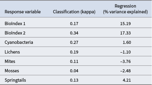
The predictive performance of the Random Forest model for each of the response variables and for both the classification and regression models is shown in Table IV. The classification models based on presence/absence performed better relative to percentage cover variables that provide an estimate of biotic density. However, the former inherently provide less information as they lack an indication of how well biotic elements are performing in a particular habitat. The regression models had reasonable performance for the BioIndex variables (> 15%), although they were comparatively poor for the individual biotic components (all < 5%). A negative score for percentage variation for lichens, mites and mosses indicates that the model performance was particularly poor.
Model performance based on the average of 100 different seed values. Negative regression values indicate that the performance of the model is lower than that of a null model.

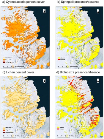
Example prediction maps for macrobiotic elements found in the Dry Valleys are shown in Fig. 4. All demonstrate the potential for modelling coverage within the study area and show that the highest predicted locations for biota are located along the edges of the valleys for cyanobacteria and springtails (Fig. 4a,b) and along the ridges between valleys for lichens (Fig. 4c). BioIndex 2 shows that, overall, biotic activity is predicted closer to the coast as well as along the edges of the valleys (Fig. 4d).
Examples of spatial prediction maps of biota from the study area in the McMurdo Dry Valleys showing a. cyanobacteria percentage cover, b. springtail presence/absence, c. lichen percentage cover and d. BioIndex 2 presence/absence.

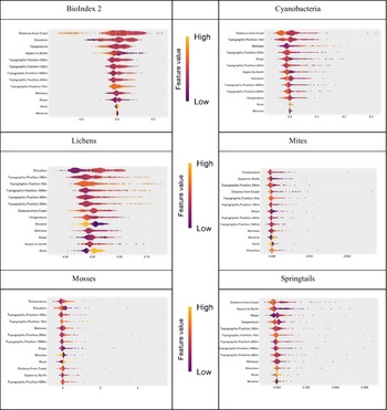
SHAP graphs for macroscopic biota in the Dry Valleys are shown in Fig. 5. For each explanatory variable and observation, the SHAP value was calculated, which quantifies the impact of the observation on the spatial model. For a given variable, each observation represents a point that is distributed horizontally along the x-axis according to its SHAP value. In places where there is a high density of SHAP values, the points are stacked vertically (resulting in a thicker shape). The variables are then ranked by their mean absolute SHAP values, which provides an indication of the influence of each variable on the model output. The colour of the individual observation points is representative of the feature’s relative observed value in the dataset from high (yellow) to low (purple), while its position (left or right of zero) represents whether the variable contributes negatively or positively, respectively, to the model’s output. The SHAP graphs provide the direction and magnitude of each variable in the model (similar to coefficients in an OLS regression model).
SHapley Additive exPlanations (SHAP) graphs for BioIndex 2 (based on presence/absence), lichens (based on percentage cover), mosses (based on percentage cover), cyanobacteria (based on percentage cover), mites (based on presence/absence) and springtails (Collembola; based on presence/absence). Values to the left of zero indicate a negative association, while those to the right are positive. The feature value colour bar indicates the relative strength of the association from high (yellow) to low (purple). Variables are listed in order of importance relative to each of the six biotic types.

For BioIndex 2, cyanobacteria and springtails, ‘Distance from Coast’ had the highest SHAP values and hence appears as the top variable. The range of yellow (high) values to the left of zero indicate the strong negative influence of distance from the coast (i.e. biota are predicted nearer the coast). Lower values to the right of zero indicate a weak positive association for some biota with distance from the coast. Elevation and temperature were also ranked highly for BioIndex 2. Lower elevations and higher temperatures positively influenced the model, and higher elevations/lower temperatures had a negative influence (Fig. 5). Lichens were somewhat different from the other biota and were positively influenced by elevation and distance from the coast and negatively influenced by wetness. Lichens obtain their water from atmospheric humidity rather than directly from glacier melt and are often located on elevated ridges, which are colder and drier, as well as more stable rock substrates (Fig. 5).
Overall, the SHAP graphs support the general expectation that warmer and wetter conditions correspond to higher levels of biotic activity. Wetness was closely linked to slope (Fig. 3), and the wetness index is influenced by water flow away from steeper ‘upstream’ areas and accumulation in downstream flatter areas. Warmer temperature results in increased snowmelt as well as providing more favourable physiological conditions in an extreme cold environment. Distance from the coast is an important explanatory variable because it correlates with higher elevations and colder temperatures (Fig. 3).
Discussion
This research used recently developed modelling techniques to explore the potential of existing NZTABS data (e.g. Lee et al. Reference Lee, Laughlin, Bottos, Caruso, Joy and Barrett2019) for predicting the spatial distribution of biota in the McMurdo Dry Valleys. Within the Antarctic literature the integration of climate-linked predictors, machine learning mapping and interpretable AI provides an advancement for modelling and spatially predicting the distribution of existing Antarctic biota. Given that the Antarctic environment is expected to change rapidly with ongoing global warming, such models can play a key role in improving our understanding and managing the consequences of this change.
The performance of our model varied depending on whether it was based on presence/absence values or a regression of percentage cover values, and also by biotic component (e.g. lichen, mite). The best model performances were achieved for the presence or absence of BioIndex 1 and BioIndex 2, cyanobacteria and lichens, with kappa varying from 0.17 to 0.34, and the only useful regression models were for BioIndex 1 and BioIndex 2 (15–17% of variance explained). Direct comparison with other modelling efforts from the same region is complicated, as not all previous models were prediction models that resulted in a distribution map. Regardless, the Lee et al. (Reference Lee, Laughlin, Bottos, Caruso, Joy and Barrett2019) study achieved a similar performance (R 2 = 0.25) for the Biodiversity Index using only GIS-derived explanatory variables. The Bottos et al. (Reference Bottos, Laughlin, Herbold, Lee, McDonald and Cary2020) model for bacterial composition had a greater R 2 of 0.43. However, this model involved directly measured variables, such as water content, pH and conductivity, which were not available as GIS layers for our study. Accordingly, the Bottos et al. (Reference Bottos, Laughlin, Herbold, Lee, McDonald and Cary2020) modelling cannot be used for larger-scale spatial prediction based on GIS layers alone.
The validation of machine learning follows a robust procedure whereby the validation data are separate from the data used to create (train) the model. This is different from the common performance measures used for OLS and structural equation models, which do not separate the training and validation data. However, having separate validation data does reduce the performance of the model. Regardless, we suggest that separating the training and validation data is likely to enable the most accurate spatial prediction to be obtained based on the current survey data and the publicly available GIS data.
Our study has focused on the availability of liquid water as an important factor predicting the distribution of terrestrial Antarctica biota. The expectation is that biotic activity will increase with increasing temperatures and increasing moisture. Our model utilizes an explicit explanatory variable based on moisture (‘wetness’) that can be fine-tuned to changes in glacier surface temperatures (degrees days > 0°C) as measured from thermal infrared satellite images. In turn, these can be used to inform future meltwater models. Having a model that is specifically connected to glacier surface temperatures enables theoretical prediction of biotic distributions based on different climate change scenarios. Assuming glacier surface temperatures can be determined from a global + 2°C climate change scenario (Paris Agreement 2015), this information can then be used to calculate an updated wetness layer. A more accurate AI spatial prediction model could then use this updated wetness layer to predict biotic responses to such change. The combination of machine leaning and explanatory SHAP graphs used in our approach adds to the knowledge of spatial modelling for Antarctic biota.
The NZTABS data are among the most comprehensive in their spatial extent as well as in the biotic variables that have been collected. Our current analysis has highlighted the usefulness of this modelling approach for the macroscopic biota. However, there are also microbiological (viral, bacterial) and microinvertebrate (nematode, tardigrade, rotifer) variables that were collected but that have yet to be fully analysed. To date, only microbiological data collected from the smaller southern Dry Valleys (Miers, Marshall and Garwood valleys) have been analysed (Bottos et al. Reference Bottos, Laughlin, Herbold, Lee, McDonald and Cary2020).
Our analysis of the NZTABS data has highlighted some shortcomings in the range of data initially collected, which we hope will be of use for designing future fieldwork. For example, the survey was stratified by elevation, slope and geology but not for moisture. Accordingly, the data lack a diversity of wet and dry habitats and have a high number of sites where the various biota are absent. The higher cumulative counts for BioIndex 1 and BioIndex 2 are likely to explain why these measures have higher model performance compared to the individual biotic components. However, this is despite BioIndex 1 and BioIndex 2 combining biotic types that have very different habitat requirements. For future field sampling efforts, particularly those supplementing existing NZTABS/Dry Valleys data, wet areas should be specifically targeted. This would result in more sites with biota (fewer ‘zeroes’), thus increasing the diversity of the data and resulting in a stronger model.
We examined a range of explanatory variables with the hope of improving the model. However, we caution that the overall spatial model should be relatively accurate prior to assessing the contributions of individual variables. For our study, only BioIndex 1 and BioIndex 2, lichen, cyanobacteria and springtail classification models were considered to have reasonable accuracy. For BioIndex 1 and BioIndex 2 (which combined all of the biotic elements), the model explanations provided by the SHAP graphs were complicated by the habitat of lichens being very different from that of the other biotic types. Specifically, lichens are not dependent on the availability of surface water and are often found on elevated sites on the crests of ridges, whereas cyanobacteria and mosses are generally found in wet sites on valley floors (Green et al. Reference Green, Sancho, Pintado and Schroeter2011, Fountain et al. Reference Fountain, Levy, Gooseff and Van Horn2014, Sohm et al. Reference Sohm, Niederberger, Parker, Tirindelli, Gunderson and Cary2020).
Indices based on topographic position from GIS layers were useful for modelling distributions for lichens and cyanobacteria. For lichens, higher values for topographic positions contribute positively to the model, especially the macro-scale topographic positions (i.e. 100 and 500 m). Positive topographic positions at these scales indicate ridges. However, for cyanobacteria, negative topographic positions positively contribute to the model, especially at the micro scale (i.e. 10 m), indicating small indentations, but also at the macro scale (i.e. 100 and 200 m), indicating valley floors. This agrees with field observations indicating that cyanobacteria are often found in low areas where water accumulates (Sohm et al. Reference Sohm, Niederberger, Parker, Tirindelli, Gunderson and Cary2020). The elevation and wetness variables are also in agreement with field observations of biota. For example, high elevation contributes positively to the presence of lichens but not to the presence of cyanobacteria. In contrast, wetness positively contributes to the presence of cyanobacteria but not to the presence of lichens. Furthermore, the SHAP graphs for lichens and cyanobacteria show that lichens correlate with stable rock and not with unstable moraine, whereas rock stability is not as important to cyanobacteria. Antarctic lichens grow very slowly and thus need relatively stable rock, whereas cyanobacteria grow more quickly and can establish in less stable areas (Brabyn et al. Reference Brabyn, Beard, Seppelt, Tuerk and Green2006, Green et al. Reference Green, Seppelt, Brabyn, Beard, Türk and Lange2015, Sohm et al. Reference Sohm, Niederberger, Parker, Tirindelli, Gunderson and Cary2020). The accuracy of explanatory AI SHAP graphs relative to known distributions of biota provides reasonable confidence that other aspects of the biota not covered as part of this study (e.g. microbes, nematodes) could also be more accurately modelled (especially compared to regression modelling). More extensive biological observations, especially in wetter locations, would greatly improve the accuracy of these predictions.
Conclusions
Here, we have described a modelling approach (Random Forest spatial prediction with SHAP explainable-AI graphics) that can be driven by satellite data (glacial surface temperatures, meltwater pathways). We also demonstrated the value of using the full range of available NZTABS data, as well as additional explanatory variables based on topography and surface stability, for spatially predicting Antarctic terrestrial biota. Given that access to liquid water is a limiting factor for Antarctic biota, and that the McMurdo Dry Valleys will become wetter with increased glacial melting, areas experiencing increased soil moisture are likely to become much more biologically active under warming scenarios. Our modelling approach can therefore be used to predict the distribution of terrestrial biota and to predict the consequences of climate change under different warming scenarios. Importantly, the model can be continually improved as more survey data become available in the future.
Acknowledgements
We are particularly grateful for the thoughtful and constructive comments of two anonymous reviewers that greatly improved the quality of the manuscript. We especially thank the many researchers who were involved in the New Zealand Terrestrial Antarctic Biocomplexity Survey (NZTABS) for their time in the field or lab, as well as for their dedication and commitment to this work. Finally, we acknowledge our friend and colleague the late Professor S.C. Cary, who led the NZTABS programme for many years following the retirement of TGAG in 2009.
Financial support
This research was supported through awards from the New Zealand Foundation for Research, Science and Technology. Logistical support for the fieldwork was provided by Antarctica New Zealand.
Competing interests
The authors declare none.
Author contributions
LB and TGAG conceived of the original research idea. LB and IDH contributed to the fieldwork, data acquisition and processing for the NZTABS project. LB and MT conducted the analysis and mapping. LB prepared the original manuscript and LB, TGAG and IDH contributed to the revised version.

 Open access