


1. Introduction
We revisit a two-sided stochastic singular control problem, where the objective is to optimally modify a stochastic process to minimize the expected net present value (NPV) of costs. In this setting, the process can be modified in both directions – increased or decreased. The total cost comprises a running cost, represented as a function f of the controlled process accumulated over time, and control costs (or rewards) proportional to the magnitude of the applied control. Problems of this kind have applications in various fields; see [Reference Avram, Kyprianou and Pistorius4, Reference Loeffen15] for examples in finance and insurance, and [Reference Dai and Yao7, Reference Dai and Yao8] for applications in inventory management.
Specifically, the state process in our problem is modeled by a spectrally negative Lévy process (i.e. Lévy process with only downward jumps). The controller can continuously increase the state process but can only decrease it at independent Poisson arrival times. The restriction on downward control to discrete times distinguishes our problem from classical studies of two-sided stochastic control, such as [Reference Baurdoux and Yamazaki5], as well as more recent work like [Reference Mordecki and Oliú18], both of which assume that controls in both directions can be applied continuously. Recently, stochastic control problems with random discrete control opportunities have received much attention in the literature; see, for example, [Reference Albrecher, Bäuerle and Thonhauser1, Reference Avanzi, Cheung, Wong and Woo3, Reference Dong, Yin and Dai9, Reference Noba, Pérez, Yamazaki and Yano19, Reference Pérez, Yamazaki and Bensoussan22, Reference Zhao, Chen and Yang24]. For recent results on Lévy processes observed at Poisson arrival times, see [Reference Albrecher, Ivanovs and Zhou2, Reference Lkabous14].
Restricting downward control opportunities to random discrete times can have useful implications in practice. For instance, in inventory management, selling is often more challenging than replenishing. While replenishment from suppliers may occur continuously, selling surplus stock might not be feasible in continuous time but instead requires some waiting period to find a suitable buyer. In such cases, modeling downward control opportunities with random discrete times is appropriate. More generally, the problem we address is applicable in situations where downward control of the stochastic process is subject to tighter constraints.
The motivation for using Poisson arrival times to model control opportunities is two-fold. First, a semi-explicit solution to the problem can be obtained by leveraging the scale functions and the exponential inter-arrival times of a Poisson process. To the best of our knowledge, explicit analytical solutions fail to exist for other types of discrete random times. In such cases numerical methods are typically employed, as the state space must be expanded to ensure the problem remains Markovian. Additionally, insights from the mathematical finance literature suggest that the solution to the constant inter-arrival model, where controls can only be applied at deterministic, uniformly spaced times, can be approximated by the solution to the Poissonian inter-arrival model. For a study on this topic, we refer readers to [Reference Leung, Yamazaki and Zhang13].
The aim of this study is to establish the optimality of a barrier strategy under the Poisson inter-arrival model. To this end, we follow the standard guess-and-verify approach:
-
(i) The NPV of costs corresponding to the periodic–classical barrier strategy is computed semi-explicitly using scale functions. The control cost has been computed in [Reference Noba, Pérez, Yamazaki and Yano19] and the running cost is computed using a result from [Reference Mata, Moreno-Franco, Noba and Pérez17].
-
(ii) The candidate barriers, denoted by $(a^*, b^*)$
, are identified using the method proposed in [Reference Noba and Yamazaki20] (see Section 3 of this work), rather than through the classical method based on the smooth-fit principle. Nevertheless, for the current problem the equivalence of the two methods is established.
$(a^*, b^*)$
, are identified using the method proposed in [Reference Noba and Yamazaki20] (see Section 3 of this work), rather than through the classical method based on the smooth-fit principle. Nevertheless, for the current problem the equivalence of the two methods is established. -
(iii) The existence and uniqueness of
$(a^*, b^*)$
is established through a probabilistic argument under a most general condition. -
(iv) The optimality of the candidate periodic–classical barrier strategy is established via a verification lemma, using a conventional argument that leverages the analytical properties of the scale functions and fluctuation identities.


While our approach leverages the scale functions of a spectrally one-sided Lévy process, several alternative methods for solving similar singular control problems have been explored in the literature. For instance, Noba and Yamazaki [Reference Noba and Yamazaki20] solve a one-sided variation of our problem for general Lévy processes. In another direction, Mordecki and Oliú [Reference Mordecki and Oliú18] address a related problem by establishing a connection to Dynkin games, under a different set of assumptions on the function f and the state process.
The remainder of this paper proceeds as follows: Section 2 presents the mathematical formulation of the problem considered. Section 3 introduces the periodic–classical barrier strategies for our problem and states the main result. Section 4 presents a sequence of results that completes the proof of the main result stated in Section 3. Section 5 presents a numerical example. Section 6 concludes this study with a discussion of several directions for potential extensions.
In this paper we use $x+$
and
$x+$
and $x-$
to denote the right- and left-hand limits at
$x-$
to denote the right- and left-hand limits at $x \in \mathbb{R}$
, respectively. Additionally, terms like strictly increasing and strictly decreasing indicate a function’s strict monotonicity, while non-decreasing and non-increasing indicate weak monotonicity. Convexity of a function is always understood in the weak sense.
$x \in \mathbb{R}$
, respectively. Additionally, terms like strictly increasing and strictly decreasing indicate a function’s strict monotonicity, while non-decreasing and non-increasing indicate weak monotonicity. Convexity of a function is always understood in the weak sense.
2. Problem setting
Defined on a probability space $(\Omega, \mathcal{F}, \mathbb{P})$
, let
$(\Omega, \mathcal{F}, \mathbb{P})$
, let $X = (X(t);\; t \geq 0)$
be a one-dimensional spectrally negative Lévy process. For
$X = (X(t);\; t \geq 0)$
be a one-dimensional spectrally negative Lévy process. For $x \in \mathbb{R}$
, we use
$x \in \mathbb{R}$
, we use $\mathbb{P}_x$
to denote the law of X with initial value x, and
$\mathbb{P}_x$
to denote the law of X with initial value x, and $\mathbb{E}_x$
to denote the corresponding expectation operator. When
$\mathbb{E}_x$
to denote the corresponding expectation operator. When $x = 0$
, we drop the subscript and simply write
$x = 0$
, we drop the subscript and simply write $\mathbb{P}$
and
$\mathbb{P}$
and $\mathbb{E}$
. The Laplace exponent of X is given by
$\mathbb{E}$
. The Laplace exponent of X is given by
 \begin{equation} \psi(s) \;:\!=\; \log\mathbb{E} \big[{\mathrm{e}}^{s X(1)}\big] = \gamma s + \frac{\sigma^2}{2} s^2 + \int_{({-}\infty, 0)} ({\mathrm{e}}^{sz} - 1 - sz\mathbf{1}_{\{z \gt -1\}})\,\mu(\mathrm{d} z), \quad s \geq 0,\end{equation}
for some $\gamma \in \mathbb{R}$
,
$\gamma \in \mathbb{R}$
, $\sigma \geq 0$
, and a Lévy measure
$\sigma \geq 0$
, and a Lévy measure $\mu$
on
$\mu$
on $({-}\infty, 0)$
satisfying
$({-}\infty, 0)$
satisfying $\int_{({-}\infty, 0)} (1 \wedge z^2) \, \mu(\mathrm{d} z) \lt \infty$
.
$\int_{({-}\infty, 0)} (1 \wedge z^2) \, \mu(\mathrm{d} z) \lt \infty$
.
The process X has paths of bounded variation if and only if $\sigma = 0$
and
$\sigma = 0$
and $\int_{({-}\infty, 0)} (1 \wedge |z|) \,\mu(\mathrm{d} z) \lt \infty$
. In the case of bounded variation, X admits the form
$\int_{({-}\infty, 0)} (1 \wedge |z|) \,\mu(\mathrm{d} z) \lt \infty$
. In the case of bounded variation, X admits the form $X(t) = \delta t - S(t)$
,
$X(t) = \delta t - S(t)$
, $t\geq 0$
, where
$t\geq 0$
, where $(S(t);\; t\geq0)$
is a subordinator and
$(S(t);\; t\geq0)$
is a subordinator and $\delta \;:\!=\; \gamma - \int_{({-}1, 0)} z\, \mu(\mathrm{d} z)$
. We assume that X is not the negative of a subordinator, and therefore
$\delta \;:\!=\; \gamma - \int_{({-}1, 0)} z\, \mu(\mathrm{d} z)$
. We assume that X is not the negative of a subordinator, and therefore $\delta \gt 0$
.
$\delta \gt 0$
.
In this paper, we consider the following singular control problem. Let $\mathcal{T}_r \;:\!=\; (T(i);\; i \geq 0)$
be the arrival times of a Poisson process
$\mathcal{T}_r \;:\!=\; (T(i);\; i \geq 0)$
be the arrival times of a Poisson process $N_r = (N_r(t);\; t \geq 0)$
with intensity
$N_r = (N_r(t);\; t \geq 0)$
with intensity $r \gt 0$
. The Poisson process
$r \gt 0$
. The Poisson process $N_r$
and its corresponding arrival times
$N_r$
and its corresponding arrival times $\mathcal{T}_r$
are independent of X. Let
$\mathcal{T}_r$
are independent of X. Let $\mathbb{F} \;:\!=\; (\mathcal{F}(t);\; t \geq 0)$
denote the (completed) filtration generated by
$\mathbb{F} \;:\!=\; (\mathcal{F}(t);\; t \geq 0)$
denote the (completed) filtration generated by $(X, N_r)$
. A strategy
$(X, N_r)$
. A strategy $\pi = \{(R^\pi(t), L^\pi(t));\; t \geq 0\}$
is a pair of non-decreasing, càdlàg, and
$\pi = \{(R^\pi(t), L^\pi(t));\; t \geq 0\}$
is a pair of non-decreasing, càdlàg, and $\mathbb{F}$
-adapted processes, with
$\mathbb{F}$
-adapted processes, with $R^\pi(0{-}) = L^\pi(0{-}) = 0$
. Under
$R^\pi(0{-}) = L^\pi(0{-}) = 0$
. Under $\pi$
, the controlled process
$\pi$
, the controlled process $Y^\pi = (Y^\pi(t);\; t \geq 0)$
is given by
$Y^\pi = (Y^\pi(t);\; t \geq 0)$
is given by
 \[Y^\pi(t) \;:\!=\; X(t) + R^\pi(t) - L^\pi(t), \quad t \geq 0.\]
Specifically, the process $R^\pi$
controls the state process in the upward direction and can be activated continuously in time, while the process
$R^\pi$
controls the state process in the upward direction and can be activated continuously in time, while the process $L^\pi$
controls it in the downward direction and can only be activated at the arrival times
$L^\pi$
controls it in the downward direction and can only be activated at the arrival times $\mathcal{T}_r$
of the Poisson process
$\mathcal{T}_r$
of the Poisson process $N_r$
. Mathematically,
$N_r$
. Mathematically, $L^\pi$
admits the form
$L^\pi$
admits the form
 \[L^\pi(t) = \int_{[0, t]}\nu^\pi(s) \, \mathrm{d} N_r(s) = \sum^\infty_{i = 1} \nu^\pi(T(i)) \mathbf{1}_{\{T(i) \leq t\}}\]
for an $\mathbb{F}$
-adapted càglàd process
$\mathbb{F}$
-adapted càglàd process $(\nu^\pi(t);\; t \geq 0)$
.
$(\nu^\pi(t);\; t \geq 0)$
.
Fix a discount factor $q \gt 0$
and an initial value
$q \gt 0$
and an initial value $x \in \mathbb{R}$
for the state process. Associated with each admissible strategy
$x \in \mathbb{R}$
for the state process. Associated with each admissible strategy $\pi$
, the NPV of costs is given by
$\pi$
, the NPV of costs is given by
 \begin{equation*} v^\pi(x) = \mathbb{E}_x \bigg[\int^\infty_0 {\mathrm{e}}^{-qt} f(Y^\pi(t))\, \mathrm{d} t + \int_{[0, \infty)} {\mathrm{e}}^{-qt}(C_{\mathrm{U}} \, \mathrm{d} R^\pi(t) + C_{\mathrm{D}} \, \mathrm{d} L^\pi(t))\bigg].\end{equation*}
Here, $f\colon \mathbb{R} \to \mathbb{R}$
is a function modeling the running cost, and
$f\colon \mathbb{R} \to \mathbb{R}$
is a function modeling the running cost, and $C_{\mathrm{U}}$
and
$C_{\mathrm{U}}$
and $C_{\mathrm{D}}$
are real numbers representing the unit costs or rewards of control. For our problem to be well-defined, we assume
$C_{\mathrm{D}}$
are real numbers representing the unit costs or rewards of control. For our problem to be well-defined, we assume
 \begin{equation} C_{\mathrm{U}} + C_{\mathrm{D}} \gt 0. \end{equation}
Assumption (2.2) is standard in the literature, such as in [Reference Baurdoux and Yamazaki5].
We impose the following assumptions.
Assumption 2.1. We assume that $f\colon \mathbb{R} \to \mathbb{R}$
satisfies the following:
$f\colon \mathbb{R} \to \mathbb{R}$
satisfies the following:
-
(i) f is a convex, piecewise continuously differentiable function. Additionally, it is assumed to be slowly or regularly varying as
$x \to \infty$
(resp.
$x \to -\infty$
) if
$\lim_{x \to \infty} |f(x)| = \infty$
(resp.
$\lim_{x \to -\infty} |f(x)| = \infty$
). -
(ii) There exists a number
$\bar{a} \;:\!=\; \inf\{a\in\mathbb{R}\colon\tilde{f}'(a) \;:\!=\; f'(a) + qC_{\mathrm{U}} \geq 0\}\in\mathbb{R}$
such that the function (2.3)is strictly decreasing on
\begin{equation} \tilde{f}(x) \;:\!=\; f(x) + qC_{\mathrm{U}}x, \quad x\in \mathbb{R}, \end{equation}
$({-}\infty, \bar{a})$
and non-decreasing on
$(\bar{a}, \infty)$
.
-
(iii) There exists a number
$\bar{\bar{a}} \;:\!=\; \inf\{a\in\mathbb{R}\colon f'(a) - qC_{\mathrm{D}} \gt 0\} \in \mathbb{R}$
.


Here and in the remainder of this paper we use f ′(x) to denote the right derivative of f at x, whenever the standard derivative does not exist.
In Assumptions 2.1, the most crucial condition is convexity, which is standard in similar singular control problems (see, for example, [Reference Baurdoux and Yamazaki5] and [Reference Pérez, Yamazaki and Bensoussan22]). The growth condition in (i) is imposed for integrability, and it is satisfied by any convex, piecewise continuously differentiable function f that is a polynomial of degree $n \geq 1$
outside a compact interval. The growth behavior of f is summarized in the following remark.
$n \geq 1$
outside a compact interval. The growth behavior of f is summarized in the following remark.
Remark 2.1. By Assumption 2.1, the running cost function f grows at most polynomially, and the derivative satisfies $f'({-}\infty) \;:\!=\; \lim_{x \to -\infty} f'(x) \in [{-}\infty, -qC_{\mathrm{U}})$
and
$f'({-}\infty) \;:\!=\; \lim_{x \to -\infty} f'(x) \in [{-}\infty, -qC_{\mathrm{U}})$
and $f'(\infty) \;:\!=\; \lim_{x \to \infty} f'(x) \in (qC_{\mathrm{D}}, \infty]$
. Moreover, by (2.2) and the convexity of f, we have
$f'(\infty) \;:\!=\; \lim_{x \to \infty} f'(x) \in (qC_{\mathrm{D}}, \infty]$
. Moreover, by (2.2) and the convexity of f, we have $\bar{a} \lt \bar{\bar{a}}$
.
$\bar{a} \lt \bar{\bar{a}}$
.
Assumptions 2.1(ii) and (iii) are imposed to avoid cases where it is optimal not to control the process from below or above. In [Reference Baurdoux and Yamazaki5], (ii) is imposed, but (iii) is not explicitly specified. The discussion for cases in which (iii) does not hold is deferred to Remark 4.2.
We also impose the following assumption for integrability. In conjunction with Assumption 2.1(i), it guarantees that $\mathbb{E}[X(1)] = \psi'(0+) \in ({-}\infty, \infty)$
and
$\mathbb{E}[X(1)] = \psi'(0+) \in ({-}\infty, \infty)$
and $\mathbb{E}_x[ \int^\infty_{0}{\mathrm{e}}^{-qs} |f(X(s))|\, \mathrm{d} s] \lt \infty$
for all
$\mathbb{E}_x[ \int^\infty_{0}{\mathrm{e}}^{-qs} |f(X(s))|\, \mathrm{d} s] \lt \infty$
for all $x \in \mathbb{R}$
.
$x \in \mathbb{R}$
.
Assumption 2.2. There exists $\theta \gt 0$
such that
$\theta \gt 0$
such that $\int_{({-}\infty, -1]} \exp(\theta |y|)\, \mu(\mathrm{d} y) \lt \infty$
.
$\int_{({-}\infty, -1]} \exp(\theta |y|)\, \mu(\mathrm{d} y) \lt \infty$
.
Let $\Pi$
be the set of admissible strategies, consisting of all
$\Pi$
be the set of admissible strategies, consisting of all $\pi$
such that:
$\pi$
such that:
-
•
$\mathbb{E}_x[\!\int^\infty_{0}{\mathrm{e}}^{-qs} |f(Y^\pi(s))|\, \mathrm{d} s] \lt \infty$
, and -
•
$\mathbb{E}_x[\!\int_{[0, \infty)}{\mathrm{e}}^{-qs}\,(\mathrm{d} R^\pi(s) + \mathrm{d} L^\pi(s))] \lt \infty$
.


The objective of this singular control problem is to compute the value function (i.e. the optimal cost function)
 \[v(x) \;:\!=\;\inf_{\pi \in \Pi} v^\pi(x), \quad x \in \mathbb{R},\]
and an associated optimal strategy $\pi^*$
such that
$\pi^*$
such that $v(x) = v^{\pi^*}(x)$
, if such a strategy exists.
$v(x) = v^{\pi^*}(x)$
, if such a strategy exists.
3. Periodic–classical barrier strategies
We now introduce the set of periodic–classical barrier strategies, comprising strategies of the form $\pi_{a,b} \;:\!=\; \{(L^{a,b}(t), R^{a,b}(t));\; t \geq 0 \}$
, parameterized by two barriers
$\pi_{a,b} \;:\!=\; \{(L^{a,b}(t), R^{a,b}(t));\; t \geq 0 \}$
, parameterized by two barriers $a \lt b$
. Under
$a \lt b$
. Under $\pi_{a, b}$
, the controlled process
$\pi_{a, b}$
, the controlled process
 \[ Y^{a,b}(t) \;:\!=\; X(t) + R^{a,b}(t) - L^{a,b}(t), \quad t \geq 0, \]
is continuously reflected from below at the lower barrier a and periodically reflected from above at the upper barrier b. In other words, the controlled process is never allowed to fall below a and is thus reflected upwards whenever it would fall below this barrier. On the other hand, at any decision time in $\mathcal{T}_r$
, if the controlled process is observed above b, it is immediately pushed down to b. The process
$\mathcal{T}_r$
, if the controlled process is observed above b, it is immediately pushed down to b. The process $Y^{a, b}$
has been studied in works such as [Reference Noba, Pérez, Yamazaki and Yano19], among others. As described in [Reference Noba, Pérez, Yamazaki and Yano19], it can be defined as a concatenation of classical reflected processes with additional downward jumps. An example is provided in Figure 1.
$Y^{a, b}$
has been studied in works such as [Reference Noba, Pérez, Yamazaki and Yano19], among others. As described in [Reference Noba, Pérez, Yamazaki and Yano19], it can be defined as a concatenation of classical reflected processes with additional downward jumps. An example is provided in Figure 1.
Left: A sample path of a spectrally negative Lévy process X. Right: The corresponding controlled process $Y^{a, b}$
with
$Y^{a, b}$
with $a = -6$
and
$a = -6$
and $b = 0$
. Vertical dashed lines indicate the Poisson arrival times
$b = 0$
. Vertical dashed lines indicate the Poisson arrival times $\mathcal{T}_r$
. Among the three arrival times displayed,
$\mathcal{T}_r$
. Among the three arrival times displayed, $Y^{a, b}$
exceeds
$Y^{a, b}$
exceeds $b = 0$
only at the second one, causing downward control to activate there but not at the first or third arrival times.
$b = 0$
only at the second one, causing downward control to activate there but not at the first or third arrival times.

Previous works, such as [Reference Baurdoux and Yamazaki5] and [Reference Pérez, Yamazaki and Bensoussan22], have shown the optimality of barrier-type strategies for one- and two-sided stochastic singular control problems by identifying an optimal barrier, or an optimal pair of barriers, according to the smooth-fit principle. For instance, in the continuous-monitoring version of this problem studied in [Reference Baurdoux and Yamazaki5], an optimal pair of barriers, denoted by $(a^*, b^*)$
, is selected such that the corresponding NPV of costs satisfies a certain smoothness condition. In this paper, we instead seek
$(a^*, b^*)$
, is selected such that the corresponding NPV of costs satisfies a certain smoothness condition. In this paper, we instead seek $(a^*, b^*)$
such that
$(a^*, b^*)$
such that $\mathfrak{C}$
holds:
$\mathfrak{C}$
holds:
 \begin{equation*} \mathfrak{C}\colon\mathbb{E}_{a^*}\bigg[\int^\infty_0{\mathrm{e}}^{-qt}f'(Y^{a^*, b^*}(t))\,\mathrm{d}t\bigg] = -C_{\mathrm{U}}, \quad \mathbb{E}_{b^*}\bigg[\int^\infty_0{\mathrm{e}}^{-qt} f'(Y^{a^*, b^*}(t))\, \mathrm{d}t\bigg] = C_{\mathrm{D}}.\end{equation*}
A similar approach was recently applied in [Reference Noba and Yamazaki20] to establish the optimality of a single-barrier strategy for the one-sided control problem considered therein. By revisiting the two-sided control problem in [Reference Baurdoux and Yamazaki5] through this approach, we can further confirm that the conditions outlined above are satisfied. Hence, although our problem is more complex than the one studied in [Reference Baurdoux and Yamazaki5], we expect that this approach will be similarly effective in identifying the optimal barriers in our setting.
The advantage of this approach is that it allows for a probabilistic interpretation. We observe that, intuitively, $\mathbb{E}_{x}\big[\int^\infty_0{\mathrm{e}}^{-qt} f'(Y^\pi(t))\,\mathrm{d}t\big]$
represents the rate of change of the running cost when the controlled process
$\mathbb{E}_{x}\big[\int^\infty_0{\mathrm{e}}^{-qt} f'(Y^\pi(t))\,\mathrm{d}t\big]$
represents the rate of change of the running cost when the controlled process $Y^\pi$
with initial value x is shifted to the right by an infinitesimal amount. Thus, it is desirable for a strategy
$Y^\pi$
with initial value x is shifted to the right by an infinitesimal amount. Thus, it is desirable for a strategy $\pi$
to keep
$\pi$
to keep $Y^{\pi}$
within the set
$Y^{\pi}$
within the set $\mathcal{C}^\pi$
for as long as possible, where
$\mathcal{C}^\pi$
for as long as possible, where
 \[\mathcal{C}^\pi \;:\!=\; \bigg\{x \in \mathbb{R}\colon -C_{\mathrm{U}} \leq \mathbb{E}_{x}\bigg[\int^\infty_0{\mathrm{e}}^{-qt} f'(Y^{\pi}(t))\, \mathrm{d} t\bigg] \leq C_{\mathrm{D}} \bigg\}.\]
We now present Theorem 3.1, the main result of this paper.
Theorem 3.1. There exists a unique pair $(a^*, b^*)$
such that
$(a^*, b^*)$
such that $\mathfrak{C}$
holds. Furthermore, the strategy
$\mathfrak{C}$
holds. Furthermore, the strategy $\pi_{a^*,b^*}$
is optimal with
$\pi_{a^*,b^*}$
is optimal with $v_{a^*, b^*}(x) = \inf_{\pi \in \Pi} v^\pi(x)$
,
$v_{a^*, b^*}(x) = \inf_{\pi \in \Pi} v^\pi(x)$
, $x\in \mathbb{R}$
, where
$x\in \mathbb{R}$
, where $v_{a^*, b^*}$
denotes the NPV of costs under the periodic–classical barrier strategy
$v_{a^*, b^*}$
denotes the NPV of costs under the periodic–classical barrier strategy $\pi_{a^*,b^*}$
.
$\pi_{a^*,b^*}$
.
The proof of Theorem 3.1 is developed in Section 4 through a series of lemmas and propositions. The existence and uniqueness of $(a^*, b^*)$
are established by first computing, and then analyzing, the expression for
$(a^*, b^*)$
are established by first computing, and then analyzing, the expression for $v_{a, b}$
for
$v_{a, b}$
for $a \lt b$
. Specifically, a semi-explicit expression for
$a \lt b$
. Specifically, a semi-explicit expression for $v_{a, b}$
is obtained using scale functions, and the pair
$v_{a, b}$
is obtained using scale functions, and the pair $(a^*, b^*)$
is identified as the solution to a pair of equations that also admit semi-explicit expressions (see (4.20)). Once existence has been established, the optimality of
$(a^*, b^*)$
is identified as the solution to a pair of equations that also admit semi-explicit expressions (see (4.20)). Once existence has been established, the optimality of $v_{a^*, b^*}$
is demonstrated through further analysis of the semi-explicit expression of
$v_{a^*, b^*}$
is demonstrated through further analysis of the semi-explicit expression of $v_{a, b}$
with
$v_{a, b}$
with $a = a^*$
and
$a = a^*$
and $b = b^*$
, in conjunction with a conventional application of Itô’s lemma. The complete proof of Theorem 3.1 is presented at the end of Section 4.
$b = b^*$
, in conjunction with a conventional application of Itô’s lemma. The complete proof of Theorem 3.1 is presented at the end of Section 4.
4. Solution
As a first step towards Theorem 3.1, we compute the expression of the NPV of costs under $\pi_{a, b}$
. To this end, we introduce the scale functions of a spectrally negative Lévy process and define several auxiliary functions that are relevant to our subsequent computations.
$\pi_{a, b}$
. To this end, we introduce the scale functions of a spectrally negative Lévy process and define several auxiliary functions that are relevant to our subsequent computations.
4.1. Scale functions and fluctuation identities
For $q \geq 0$
, the scale function
$q \geq 0$
, the scale function $W^{(q)}\colon \mathbb{R} \to [0 , \infty)$
of the spectrally negative Lévy process X is defined as follows. On the negative half-line,
$W^{(q)}\colon \mathbb{R} \to [0 , \infty)$
of the spectrally negative Lévy process X is defined as follows. On the negative half-line, $W^{(q)}$
is set to be zero. On the positive half-line, it is a continuous and strictly increasing function that satisfies
$W^{(q)}$
is set to be zero. On the positive half-line, it is a continuous and strictly increasing function that satisfies
 \begin{align} \int^\infty_0 {\mathrm{e}}^{-\theta x} W^{(q)}(x)\, \mathrm{d} x = \frac{1}{\psi(\theta) - q}, \quad \theta \gt \Phi_q.\end{align}
Here, $\psi$
is the Laplace exponent defined in (2.1), and
$\psi$
is the Laplace exponent defined in (2.1), and $\Phi_q \;:\!=\; \sup \{s \geq 0\colon \psi(s) = q\}$
,
$\Phi_q \;:\!=\; \sup \{s \geq 0\colon \psi(s) = q\}$
, $q \geq 0$
, is its right inverse. We refer the readers to [Reference Kuznetsov, Kyprianou and Rivero11, Reference Kyprianou12] for a comprehensive review of scale functions. In particular, [Reference Kuznetsov, Kyprianou and Rivero11, Lemmas 2.3, 2.4, 3.1, and 3.2], which expound the smoothness of the scale functions, are of particular importance.
$q \geq 0$
, is its right inverse. We refer the readers to [Reference Kuznetsov, Kyprianou and Rivero11, Reference Kyprianou12] for a comprehensive review of scale functions. In particular, [Reference Kuznetsov, Kyprianou and Rivero11, Lemmas 2.3, 2.4, 3.1, and 3.2], which expound the smoothness of the scale functions, are of particular importance.
We define, for $x \in \mathbb{R}$
,
$x \in \mathbb{R}$
,
 \begin{equation*} \overline{W}^{(q)}(x) \;:\!=\; \int_0^{x} W^{(q)}(y)\, \mathrm{d} y, \qquad \overline{\overline{W}}^{(q)}(x) \;:\!=\; \int_0^{x} \overline{W}^{(q)}(y)\, \mathrm{d} y.\end{equation*}
For $x \in \mathbb{R}$
and
$x \in \mathbb{R}$
and $r \gt 0$
, we also define the second scale function,
$r \gt 0$
, we also define the second scale function,
 \begin{equation} Z^{(q)}(x,\Phi_{q + r}) \;:\!=\; {\mathrm{e}}^{\Phi_{q + r}x}\bigg(1-r\int_0^{x}{\mathrm{e}}^{-\Phi_{q + r}z}W^{(q)}(z)\,\mathrm{d}z\bigg) = r\int_0^{\infty}{\mathrm{e}}^{-\Phi_{q + r}z}W^{(q)}(z + x)\,\mathrm{d}z,\end{equation}
where the second equality holds because (4.1) gives $\int^\infty_0\mathrm{e}^{-\Phi_{q+r} x} W^{(q)}(x) \, \mathrm{d} x = r^{-1}$
. Differentiating the second scale function with respect to the first argument, we obtain
$\int^\infty_0\mathrm{e}^{-\Phi_{q+r} x} W^{(q)}(x) \, \mathrm{d} x = r^{-1}$
. Differentiating the second scale function with respect to the first argument, we obtain
 \begin{equation*} Z^{(q)'}(x,\Phi_{q+r}) \;:\!=\; \frac{\partial}{\partial x} Z^{(q)}(x,\Phi_{q+r}) = \Phi_{q+r} Z^{(q)}(x,\Phi_{q+r}) - rW^{(q)}(x), \quad x \gt 0. \end{equation*}
Moreover, for $q\geq 0$
and
$q\geq 0$
and $x \in \mathbb{R}$
, we define
$x \in \mathbb{R}$
, we define
 \begin{equation*} Z^{(q)}(x) \;:\!=\; 1 + q\overline{W}^{(q)}(x), \qquad \overline{Z}^{(q)}(x) \;:\!=\; \int^x_0 Z^{(q)}(y)\, \mathrm{d} y = x + q \overline{\overline{W}}^{(q)}(x).\end{equation*}
For $b \gt a$
,
$b \gt a$
, $x \in \mathbb{R}$
, and
$x \in \mathbb{R}$
, and $h\colon \mathbb{R} \to \mathbb{R}$
, we define
$h\colon \mathbb{R} \to \mathbb{R}$
, we define
 \begin{align} \rho_{a, b}^{(q)}(x;\; h) & \;:\!=\; \int^{b}_a W^{(q)}(x - y)h(y)\, \mathrm{d} y, \end{align}
 \begin{align} \rho_{a, b}^{(q, r)}(x;\; h) & \;:\!=\; \rho_{a, b}^{(q)}(x;\; h) + r\int^{x}_bW^{(q + r)}(x - y)\rho_{a, b}^{(q)}(y;\; h)\,\mathrm{d}y. \end{align}
Additionally, for $x \in \mathbb{R}$
, we define
$x \in \mathbb{R}$
, we define
 \begin{align} W^{(q, r)}_{a, b}(x) & \;:\!=\; W^{(q)}(x - a) + r\int^x_b W^{(q + r)}(x - y)W^{(q)}(y - a)\,\mathrm{d}y, \end{align}
 \begin{align} Z^{(q, r)}_{a, b}(x) & \;:\!=\; Z^{(q)}(x - a) + r\int^x_bW^{(q + r)}(x - y)Z^{(q)}(y - a)\,\mathrm{d}y, \end{align}
 \begin{align} \overline{Z}^{(q, r)}_{a, b}(x) & \;:\!=\; \overline{Z}^{(q)}(x - a) + r\int^x_bW^{(q + r)}(x - y)\overline{Z}^{(q)}(y - a)\,\mathrm{d}y. \end{align}
It is convenient to decompose the NPV of costs into the following two components, both of which can be expressed in terms of the scale functions $W^{(q)}$
and
$W^{(q)}$
and $W^{(q + r)}$
, as well as the auxiliary functions defined above:
$W^{(q + r)}$
, as well as the auxiliary functions defined above:
 \begin{equation*} v_{a,b}(x) = v_{a, b}^{LR}(x) + v_{a, b}^{f}(x), \quad x\in \mathbb{R},\end{equation*}
where
 \begin{align*} v_{a, b}^{LR}(x) & \;:\!=\; C_{\mathrm{D}}\mathbb{E}_{x}\bigg[\int_{[0,\infty)}{\mathrm{e}}^{-qt}\,\mathrm{d}L^{a, b}(t)\bigg] + C_{\mathrm{U}}\mathbb{E}_{x}\bigg[\int_{[0,\infty)}{\mathrm{e}}^{-qt}\,\mathrm{d}R^{a, b}(t)\bigg], \\[5pt] v_{a, b}^{f}(x) & \;:\!=\; \mathbb{E}_x\bigg[\int^\infty_0{\mathrm{e}}^{-qt} f(Y^{a, b}(t))\,\mathrm{d}t\bigg].\end{align*}
To compute $v_{a, b}^{LR}$
, we apply the result established in the proof of [Reference Noba, Pérez, Yamazaki and Yano19, Lemma 3.1], which expresses
$v_{a, b}^{LR}$
, we apply the result established in the proof of [Reference Noba, Pérez, Yamazaki and Yano19, Lemma 3.1], which expresses $v_{0, b}^{LR}$
for
$v_{0, b}^{LR}$
for $b \gt 0$
in terms of the scale functions and the auxiliary functions.
$b \gt 0$
in terms of the scale functions and the auxiliary functions.
Lemma 4.1 ([Reference Noba, Pérez, Yamazaki and Yano19, Lemma 3.1].) For $a \lt b$
and
$a \lt b$
and $x \in \mathbb{R}$
,
$x \in \mathbb{R}$
,
 \begin{align} v_{a, b}^{LR}(x) & = \bigg(\frac{r}{q\Phi_{q+r}}\frac{C_{\mathrm{U}}Z^{(q)}(b-a) + C_{\mathrm{D}}}{Z^{(q)}(b-a,\Phi_{q+r})} + \frac{C_{\mathrm{U}}}{\Phi_{q+r}}\bigg)\Big(Z^{(q,r)}_{a,b}(x) - rZ^{(q)}(b-a)\overline{W}^{(q+r)}(x - b)\Big) \nonumber \\[5pt] & \quad - rC_{\mathrm{D}}\overline{\overline{W}}^{(q+r)}(x - b) - C_{\mathrm{U}}\bigg(\overline{Z}^{(q,r)}_{a,b}(x) + \frac{\psi'(0+)}{q} - r\overline{Z}^{(q)}(b - a) \overline{W}^{(q + r)}(x - b)\bigg). \end{align}
The running cost $v_{a, b}^{f}$
is computed using [Reference Mata, Moreno-Franco, Noba and Pérez17, Proposition 5.1]. Details of the computation are given in Appendix A.1.
$v_{a, b}^{f}$
is computed using [Reference Mata, Moreno-Franco, Noba and Pérez17, Proposition 5.1]. Details of the computation are given in Appendix A.1.
Lemma 4.2. For $a \lt b$
and
$a \lt b$
and $x \in \mathbb{R}$
,
$x \in \mathbb{R}$
,
 \begin{align} v_{a, b}^{f}(x) & = \frac{1}{q}\bigg(f(a) + \int^{\infty}_af'(y)\frac{Z^{(q)}(b-y,\Phi_{q+r})}{Z^{(q)}(b-a,\Phi_{q+r})}\,\mathrm{d}y\bigg) Z^{(q, r)}_{a, b}(x) - \rho_{a, b}^{(q, r)}(x;\kern3pt f) \nonumber \\[5pt] & \quad -r\overline{W}^{(q+r)}(x-b)v_{a,b}^{f}(b) - \int^{x}_bf(y)W^{(q+r)}(x-y)\,\mathrm{d}y, \end{align}
where
 \begin{equation*} v_{a, b}^{f}(b) = -\rho_{a, b}^{(q)}(b;\kern3pt f) + \frac{1}{q}\bigg(f(a) + \int^{\infty}_af'(y)\frac{Z^{(q)}(b-y, \Phi_{q+r})}{Z^{(q)}(b-a,\Phi_{q+r})}\, \mathrm{d}y\bigg)Z^{(q)}(b - a). \end{equation*}
Combining (4.8) and (4.9), and applying integration by parts, we obtain Lemma 4.3, with the proof provided in Appendix A.2. Recall $\tilde{f}$
as defined in (2.3).
$\tilde{f}$
as defined in (2.3).
Lemma 4.3. For $a \lt b$
and
$a \lt b$
and $x \in \mathbb{R}$
,
$x \in \mathbb{R}$
,
 \begin{align} v_{a,b}(x) & = \frac{1}{q}\bigg(\tilde{f}(a) + \frac{\Gamma(a, b)}{Z^{(q)}(b - a, \Phi_{q + r})}\bigg) \big(Z^{(q, r)}_{a, b}(x) - r\overline{W}^{(q + r)}(x - b)Z^{(q)}(b - a) \big)\nonumber \\[5pt] & \quad - r(C_{\mathrm{U}} + C_{\mathrm{D}})\overline{\overline{W}}^{(q + r)}(x - b) - C_{\mathrm{U}}x + r\overline{W}^{(q+r)}(x-b)\rho_{a,b}^{(q)}(b;\,\tilde{f}) \nonumber \\[5pt]& \quad - \tilde{f}(b)\overline{W}^{(q+r)}(x-b) - \rho_{a, b}^{(q, r)}(x;\ \tilde{f}) - C_{\mathrm{U}}\frac{\psi'(0+)}{q} - \int^{x}_b\overline{W}^{(q + r)}(x - y)\tilde{f}'(y)\,\mathrm{d}y, \end{align}
where
 \begin{equation} \Gamma(a, b) \;:\!=\; \int^{\infty}_a \tilde{f}'(y) Z^{(q)}(b - y, \Phi_{q + r})\, \mathrm{d} y + \frac{r}{\Phi_{q + r}} (C_{\mathrm{U}} + C_{\mathrm{D}}), \quad a \lt b. \end{equation}
4.2. Smoothness of
$\boldsymbol{{v}}_{\boldsymbol{{a, b}}}$

We now analyze the smoothness of the NPV of costs as computed in (4.10).
Lemma 4.4. For $a \lt b$
and
$a \lt b$
and $x \in \mathbb{R}\backslash \{a\}$
,
$x \in \mathbb{R}\backslash \{a\}$
,
 \begin{align} v'_{a, b}(x) & = \frac{\Gamma(a, b)}{Z^{(q)}(b - a, \Phi_{q + r})} W^{(q, r)}_{a, b}(x) - \rho_{a, b}^{(q, r)}(x;\kern3pt \tilde{f}') \nonumber \\[5pt] & \quad - \int^{x}_{b} W^{(q + r)}(x - y) \tilde{f}'(y)\, \mathrm{d} y - r(C_{\mathrm{U}} + C_{\mathrm{D}}) \overline{W}^{(q + r)}(x - b) - C_{\mathrm{U}}. \end{align}
If X is of unbounded variation, for $a \lt b$
and
$a \lt b$
and $x \in \mathbb{R}\backslash \{a\}$
,
$x \in \mathbb{R}\backslash \{a\}$
,
 \begin{align} v''_{a, b}(x) & = \frac{\Gamma(a,b)}{Z^{(q)}(b-a,\Phi_{q+r})}\bigg(\frac{\mathrm{d}}{\mathrm{d}x}W^{(q,r)}_{a,b}(x)\bigg) \nonumber \\[5pt] & \quad - \bigg(\int^{b}_a W^{(q)'}(x - y)\tilde{f}'(y)\, \mathrm{d} y + r\int^{x}_b W^{(q + r)'}(x - y)\rho_{a, b}^{(q)}(y;\; \tilde{f}')\, \mathrm{d} y\bigg) \nonumber \\[5pt] & \quad - \int^{x}_{b} W^{(q + r)'}(x - y) \tilde{f}'(y)\, \mathrm{d} y - r(C_{\mathrm{U}} + C_{\mathrm{D}}) W^{(q + r)}(x - b). \end{align}
The proof of Lemma 4.4 is provided in Appendix A.3. The derivative $({\mathrm{d}}/{\mathrm{d}x})W^{(q, r)}_{a, b}(x)$
in (4.13) is well-defined for
$({\mathrm{d}}/{\mathrm{d}x})W^{(q, r)}_{a, b}(x)$
in (4.13) is well-defined for $x \neq a$
in light of (4.5) and the smoothness of scale functions as in [Reference Kuznetsov, Kyprianou and Rivero11, Lemma 2.4]. In the remainder of this paper, we call a function sufficiently smooth if it is continuously differentiable on
$x \neq a$
in light of (4.5) and the smoothness of scale functions as in [Reference Kuznetsov, Kyprianou and Rivero11, Lemma 2.4]. In the remainder of this paper, we call a function sufficiently smooth if it is continuously differentiable on $\mathbb{R}$
when X is of bounded variation and twice continuously differentiable on
$\mathbb{R}$
when X is of bounded variation and twice continuously differentiable on $\mathbb{R}$
when X is of unbounded variation.
$\mathbb{R}$
when X is of unbounded variation.
The following results establish the equivalence between our approach and the classical approach based on the smooth-fit principle.
Proposition 4.1. For $a \lt b$
, the function
$a \lt b$
, the function $x \mapsto v_{a, b}(x)$
is sufficiently smooth if and only if
$x \mapsto v_{a, b}(x)$
is sufficiently smooth if and only if $\Gamma(a,b) = 0$
.
$\Gamma(a,b) = 0$
.
Proof. By Lemma 4.4, we have
 \begin{equation*} v'_{a, b}(a{-}) = -C_{\mathrm{U}}, \qquad v'_{a, b}(a+) = -C_{\mathrm{U}} + \frac{\Gamma(a, b)}{Z^{(q)}(b - a, \Phi_{q + r})} W^{(q)}(0) \end{equation*}
in the case that X is of bounded variation, and
 \begin{equation*} v''_{a, b}(a{-}) = 0, \qquad v''_{a, b}(a+) = \frac{\Gamma(a, b)}{Z^{(q)}(b - a, \Phi_{q + r})} W^{(q)'}(0{+}) \end{equation*}
when X is of unbounded variation. Now, by applying [Reference Kuznetsov, Kyprianou and Rivero11, Lemmas 3.1 and 3.2], we find that the function $x \mapsto v_{a, b}(x)$
is sufficiently smooth if and only if
$x \mapsto v_{a, b}(x)$
is sufficiently smooth if and only if $\Gamma(a,b) = 0$
.
$\Gamma(a,b) = 0$
.
Define the partial derivative of $\Gamma$
as follows:
$\Gamma$
as follows:
 \begin{align} \gamma(a, b) \;:\!=\; \frac{\partial}{\partial b} \Gamma(a, b) & = \Phi_{q+r}\int^{\infty}_a\tilde{f}'(y)Z^{(q)}(b - y,\Phi_{q + r})\,\mathrm{d}y - r\rho_{a, b}^{(q)}(b;\kern3pt \tilde{f}') \nonumber \\[5pt]& = \Phi_{q+r}\Gamma(a,b) - r\big(C_{\mathrm{U}} + C_{\mathrm{D}} + \rho_{a,b}^{(q)}(b;\kern3pt \tilde{f}')\big), \quad a \lt b. \end{align}
Note that $\gamma(a, b)$
is independent of the values of
$\gamma(a, b)$
is independent of the values of $C_{\mathrm{U}}$
and
$C_{\mathrm{U}}$
and $C_{\mathrm{D}}$
, as the second equality of (4.14) holds by adding and subtracting
$C_{\mathrm{D}}$
, as the second equality of (4.14) holds by adding and subtracting $r(C_{\mathrm{U}} + C_{\mathrm{D}})$
, together with (4.11). This equality is included only to simplify complex expressions that appear later in the paper. The proof of Lemma 4.2 is presented in Appendix A.4.
$r(C_{\mathrm{U}} + C_{\mathrm{D}})$
, together with (4.11). This equality is included only to simplify complex expressions that appear later in the paper. The proof of Lemma 4.2 is presented in Appendix A.4.
Lemma 4.5. For $a \lt b$
and
$a \lt b$
and $x \in \mathbb{R}$
, we have
$x \in \mathbb{R}$
, we have
 \begin{align} v^{f'}_{a, b}(x) & \;:\!=\; \mathbb{E}_x\bigg[\int^\infty_0{\mathrm{e}}^{-qt} f'(Y^{a, b}(t))\,\mathrm{d}t\bigg] \nonumber \\[5pt]& = \frac{\gamma(a,b)}{qZ^{(q)}(b-a;\,\Phi_{q+r})}Z^{(q,r)}_{a,b}(x) - \rho_{a, b}^{(q, r)}(x;\kern3pt \tilde{f}') - \int^{x}_b W^{(q + r)}(x - y)\,\tilde{f}'(y)\,\mathrm{d}y \nonumber \\[5pt]& \quad - r\overline{W}^{(q + r)}(x - b)\bigg({-}\rho_{a b}^{(q)}(b;\kern3pt \tilde{f}') + \frac{Z^{(q)}(b - a)}{qZ^{(q)}(b - a;\; \Phi_{q + r})}\gamma(a, b)\bigg) - C_{\mathrm{U}}. \end{align}
In particular, at $x = a$
and
$x = a$
and $x = b$
,
$x = b$
,
 \begin{align} v^{f'}_{a, b}(a) & = \frac{\gamma(a, b)}{qZ^{(q)}(b - a;\; \Phi_{q + r})} - C_{\mathrm{U}}, \end{align}
 \begin{align} v^{f'}_{a, b}(b) & = \frac{Z^{(q)}(b - a)}{qZ^{(q)}(b - a;\; \Phi_{q + r})}\gamma(a, b) - \rho_{a, b}^{(q)}(b;\; \tilde{f}') - C_{\mathrm{U}}. \end{align}
Proposition 4.2. For $a \lt b$
, the following statements are equivalent:
$a \lt b$
, the following statements are equivalent:
-
(i)
$v^{f'}_{a, b}(a) = -C_{\mathrm{U}}$
and
$v^{f'}_{a, b}(b) = C_{\mathrm{D}}$
. -
(ii)
$\Gamma(a, b) = 0$
and
$\gamma(a,b) = 0$
. -
(iii)
$v_{a, b}$
is sufficiently smooth, with
$v'_{a, b}(a) = -C_{\mathrm{U}}$
and
$v'_{a, b}(b) = C_{\mathrm{D}}$
.


Proof. For (i) $\Longleftrightarrow$
(ii), first, by (4.16),
$\Longleftrightarrow$
(ii), first, by (4.16),
 \begin{equation} v^{f'}_{a, b}(a) = -C_{\mathrm{U}} \Longleftrightarrow \gamma(a, b) = 0. \end{equation}
By (4.14), we have
 \begin{equation} \rho_{a, b}^{(q)}(b;\; \tilde{f}') = \frac{\Phi_{q+r}\Gamma(a, b) - \gamma(a,b)}r - (C_{\mathrm{U}} + C_{\mathrm{D}}) . \end{equation}
Substituting (4.19) into (4.17), we have
 \begin{equation*} v^{f'}_{a, b}(b) = -\frac{\Phi_{q+r}}{r}\Gamma(a, b) + \bigg(\frac{Z^{(q)}(b-a)}{qZ^{(q)}(b-a;\,\Phi_{q+r})} + \frac{1}{r}\bigg)\gamma(a,b) + C_{\mathrm{D}}. \end{equation*}
The equivalence follows from the last equality and (4.18).
For (ii) $\Longleftrightarrow$
(iii), substituting (4.19) in (4.12) with
$\Longleftrightarrow$
(iii), substituting (4.19) in (4.12) with $x = b$
,
$x = b$
,
 \begin{equation*} v'_{a, b}(b) = \bigg(\frac{W^{(q)}(b-a)}{Z^{(q)}(b-a,\Phi_{q+r})} - \frac{\Phi_{q+r}}{r}\bigg)\Gamma(a,b) + \frac{\gamma(a, b)}{r} + C_{\mathrm{D}}. \end{equation*}
Thus, $v'_{a, b}(b) = C_{\mathrm{D}}$
is equivalent to
$v'_{a, b}(b) = C_{\mathrm{D}}$
is equivalent to $\gamma(a, b) = 0$
when
$\gamma(a, b) = 0$
when $\Gamma(a, b) = 0$
. Finally, Lemma 4.1 shows the equivalence.
$\Gamma(a, b) = 0$
. Finally, Lemma 4.1 shows the equivalence.
4.3. Selection of barriers
The next step of our analysis involves establishing the existence of $(a^*, b^*)$
satisfying
$(a^*, b^*)$
satisfying
 \begin{equation*} \mathfrak{C}\colon v^{f'}_{a^*, b^*}(a^*) = -C_{\mathrm{U}} \quad \textrm{and} \quad v^{f'}_{a^*, b^*}(b^*) = C_{\mathrm{D}},\end{equation*}
which is, by Proposition 4.2, equivalent to
 \begin{equation} \mathfrak{C}'\colon \Gamma(a^*,b^*) = \gamma(a^*, b^*) = 0.\end{equation}
Recall $\bar{a} = \inf\{a \in \mathbb{R}\colon \tilde{f}'(a) \geq 0\}$
as defined in Assumption 2.1(ii). We can immediately eliminate the half-line
$\bar{a} = \inf\{a \in \mathbb{R}\colon \tilde{f}'(a) \geq 0\}$
as defined in Assumption 2.1(ii). We can immediately eliminate the half-line $[\bar{a}, \infty)$
from consideration for
$[\bar{a}, \infty)$
from consideration for $a^*$
. Indeed, for
$a^*$
. Indeed, for $a \geq \overline{a}$
, we have
$a \geq \overline{a}$
, we have $\tilde{f}'(y + a) \geq \tilde{f}'(y + \bar{a}) \geq 0$
for all
$\tilde{f}'(y + a) \geq \tilde{f}'(y + \bar{a}) \geq 0$
for all $y \geq 0$
by Assumption 2.1(i). Thus, from (4.11), we have
$y \geq 0$
by Assumption 2.1(i). Thus, from (4.11), we have $\Gamma(a, b) \gt 0$
for
$\Gamma(a, b) \gt 0$
for $b \gt a \geq \bar{a}$
. We show that, by decreasing the value of a from
$b \gt a \geq \bar{a}$
. We show that, by decreasing the value of a from $\bar{a}$
, we reach
$\bar{a}$
, we reach $a^*$
such that the function
$a^*$
such that the function $b \mapsto \Gamma(a^*, b)$
starts at
$b \mapsto \Gamma(a^*, b)$
starts at $\Gamma(a^*, a^*+) \gt 0$
and becomes tangent to the x-axis at
$\Gamma(a^*, a^*+) \gt 0$
and becomes tangent to the x-axis at $b^*$
, where its partial derivative
$b^*$
, where its partial derivative $\gamma(a^*, b^*)$
is zero.
$\gamma(a^*, b^*)$
is zero.
To facilitate the proof of the existence of $(a^*, b^*)$
, we analyze the following auxiliary functions.
$(a^*, b^*)$
, we analyze the following auxiliary functions.
Lemma 4.6. For all $a \in \mathbb{R}$
,
$a \in \mathbb{R}$
,
 \begin{align} \Gamma_1(a) & \;:\!=\; \Gamma(a, a{+}) = \int^\infty_0{\mathrm{e}}^{-\Phi_{q + r} y} \tilde{f}'(y+a) \, \mathrm{d} y + \frac{r}{\Phi_{q+r}}(C_{\mathrm{U}} + C_{\mathrm{D}}), \end{align}
 \begin{align} \Gamma_2(a) & \;:\!=\; \lim_{b \to \infty} \frac{\Gamma(a, b)}{Z^{(q)}(b - a, \Phi_{q + r})} = \int^{\infty}_0{\mathrm{e}}^{-\Phi_q y} \tilde{f}'(y + a)\, \mathrm{d} y. \end{align}
The proof of Lemma 4.6 is deferred to Appendix A.5. We note that both $a\mapsto \Gamma_1(a)$
and
$a\mapsto \Gamma_1(a)$
and $a\mapsto \Gamma_2(a)$
are continuous. Moreover, both are strictly increasing on
$a\mapsto \Gamma_2(a)$
are continuous. Moreover, both are strictly increasing on $({-}\infty, \bar{a})$
due to the convexity of
$({-}\infty, \bar{a})$
due to the convexity of $\tilde{f}$
and Assumption 2.1(iii). Define their left inverses,
$\tilde{f}$
and Assumption 2.1(iii). Define their left inverses,
 \begin{equation} \underline{a}_i \;:\!=\; \inf\{a \in \mathbb{R}\colon \Gamma_i(a) \geq 0\}, \quad i = 1,2.\end{equation}
Observe that $\underline{a}_1 \in [{-}\infty, \bar{a})$
and
$\underline{a}_1 \in [{-}\infty, \bar{a})$
and $\underline{a}_2 \in ({-}\infty, \bar{a}).$
To establish that
$\underline{a}_2 \in ({-}\infty, \bar{a}).$
To establish that $\underline{a}_2 \gt -\infty$
, note that by monotone convergence and the convexity of
$\underline{a}_2 \gt -\infty$
, note that by monotone convergence and the convexity of $\tilde{f}$
, we have
$\tilde{f}$
, we have $\Gamma_2(a) \xrightarrow{a \downarrow -\infty}\int^{\infty}_0{\mathrm{e}}^{-\Phi_q z} \tilde{f}'({-}\infty)\, \mathrm{d} z \in [{-}\infty, 0)$
. Hence,
$\Gamma_2(a) \xrightarrow{a \downarrow -\infty}\int^{\infty}_0{\mathrm{e}}^{-\Phi_q z} \tilde{f}'({-}\infty)\, \mathrm{d} z \in [{-}\infty, 0)$
. Hence, $\underline{a}_2 \gt -\infty$
. To show that both
$\underline{a}_2 \gt -\infty$
. To show that both $\underline{a}_1$
and
$\underline{a}_1$
and $\underline{a}_2$
are upper bounded by
$\underline{a}_2$
are upper bounded by $\bar{a}$
, note that by (2.2) and Assumption 2.1(ii), we have
$\bar{a}$
, note that by (2.2) and Assumption 2.1(ii), we have
 \[ \Gamma_1(\bar{a}) = \int^\infty_0{\mathrm{e}}^{-\Phi_{q + r} y} \tilde{f}'(y + \bar{a})\, \mathrm{d} y + \frac{r}{\Phi_{q + r}}(C_{\mathrm{U}} + C_{\mathrm{D}}) \gt 0,\]
which implies $\bar{a} \gt \underline{a}_1$
. Additionally, by Assumption 2.1(iii),
$\bar{a} \gt \underline{a}_1$
. Additionally, by Assumption 2.1(iii), $\Gamma_2(\bar{a}) \gt 0$
, which implies
$\Gamma_2(\bar{a}) \gt 0$
, which implies $\bar{a} \gt \underline{a}_2$
.
$\bar{a} \gt \underline{a}_2$
.
Remark 4.1. The value $\underline{a}_2$
is the optimal barrier in the setting where only upward control is permitted; see [Reference Yamazaki23, Section 7]. This follows from the definition of
$\underline{a}_2$
is the optimal barrier in the setting where only upward control is permitted; see [Reference Yamazaki23, Section 7]. This follows from the definition of $\underline{a}_2$
in (4.23), which gives
$\underline{a}_2$
in (4.23), which gives
 \begin{equation*} 0 = \frac{\Phi_{q}}{q}\Gamma_2(\underline{a}_2) = \frac{\Phi_{q}}{q}\int^\infty_0{\mathrm{e}}^{-\Phi_{q}y}f'(y + \underline{a}_2)\,\mathrm{d}y + C_{\mathrm{U}} = \mathbb{E}_{\underline{a}_2}\bigg[\int^\infty_0{\mathrm{e}}^{-qt}f'(Y^{\underline{a}_2,\infty}(t))\,\mathrm{d}t\bigg] + C_{\mathrm{U}}, \end{equation*}
where $Y^{\underline{a}_2, \infty}$
denotes the process reflected from below at the level
$Y^{\underline{a}_2, \infty}$
denotes the process reflected from below at the level $\underline{a}_2$
, and the last equality holds by [Reference Kuznetsov, Kyprianou and Rivero11, Theorem 2.8(iii)]. Thus,
$\underline{a}_2$
, and the last equality holds by [Reference Kuznetsov, Kyprianou and Rivero11, Theorem 2.8(iii)]. Thus,
 \begin{align} \mathbb{E}_{\underline{a}_2}\bigg[\int^\infty_0{\mathrm{e}}^{-qt}f'(Y^{\underline{a}_2,\infty}(t))\,\mathrm{d}t\bigg] = -C_{\mathrm{U}}. \end{align}
Moreover, under certain conditions in our current setting, an optimal strategy is the barrier strategy that continuously reflects the state process from below at the lower barrier $\underline{a}_2$
, as summarized in the following remark.
$\underline{a}_2$
, as summarized in the following remark.
Remark 4.2. Suppose that Assumption 2.1(iii) fails to hold (thus $f' \leq qC_{\mathrm{D}}$
on
$f' \leq qC_{\mathrm{D}}$
on $\mathbb{R}$
) and all other standing assumptions, including Assumptions 2.1(i) and (ii), hold. Then,
$\mathbb{R}$
) and all other standing assumptions, including Assumptions 2.1(i) and (ii), hold. Then,
-
• not activating the downward control
$(L^\pi(t);\; t \geq 0)$
is optimal; -
•
$v_{\underline{a}_2, \infty}(x) = \inf_{\pi \in \Pi} v^\pi(x)$
for all
$x \in \mathbb{R}$
, where
\begin{equation*} v_{\underline{a}_2, \infty}(x) \;:\!=\; \mathbb{E}_x\bigg[\int^\infty_0{\mathrm{e}}^{-qt}f(Y^{\underline{a}_2,\infty}(t))\,\mathrm{d}t + C_{\mathrm{U}}\int_{[0,\infty)}{\mathrm{e}}^{-qt}\,\mathrm{d}R^{\underline{a}_2,\infty}(t)\bigg]. \end{equation*}


Verifying the above remark is straightforward. The first statement holds since the downward control cost is no less than the reduction in the running cost. The second statement holds due to the first and [Reference Yamazaki23, Theorem 7.1].
As a next step towards establishing the existence of $(a^*, b^*)$
, we define
$(a^*, b^*)$
, we define
 \[ \underline{\Gamma}(a) \;:\!=\; \inf_{b \gt a} \Gamma(a, b), \quad a \in \mathbb{R}.\]
The proofs of the following two lemmas are provided in Appendices A.6 and A.7.
Lemma 4.7. (i) $\underline{\Gamma}(\bar{a}) \gt 0$
; (ii)
$\underline{\Gamma}(\bar{a}) \gt 0$
; (ii) $\underline{\Gamma}(\underline{a}_1 \vee \underline{a}_2) \lt 0$
.
$\underline{\Gamma}(\underline{a}_1 \vee \underline{a}_2) \lt 0$
.
Lemma 4.8. The mapping $a \mapsto \underline{\Gamma}(a)$
is continuous and strictly increasing on
$a \mapsto \underline{\Gamma}(a)$
is continuous and strictly increasing on $(\underline{a}_1 \vee \underline{a}_2, \bar{a})$
.
$(\underline{a}_1 \vee \underline{a}_2, \bar{a})$
.
We are now ready to establish the existence and uniqueness of the candidate barriers.
Proposition 4.3. There exists a unique pair $(a^*, b^*)$
such that
$(a^*, b^*)$
such that $\mathfrak{C}$
holds.
$\mathfrak{C}$
holds.
Proof. By Lemmas 4.7 and 4.8, there exists a unique root $a^* \in (\underline{a}_1 \vee \underline{a}_2, \infty)$
such that
$a^* \in (\underline{a}_1 \vee \underline{a}_2, \infty)$
such that $\underline{\Gamma}(a^*) = 0$
. Moreover, because
$\underline{\Gamma}(a^*) = 0$
. Moreover, because $\Gamma(a^*, a^*+) \gt 0$
and
$\Gamma(a^*, a^*+) \gt 0$
and $\lim_{b \to \infty}\Gamma(a^*,b) = \infty$
in view of the definitions of
$\lim_{b \to \infty}\Gamma(a^*,b) = \infty$
in view of the definitions of $\underline{a}_1$
and
$\underline{a}_1$
and $\underline{a}_2$
, the minimum of
$\underline{a}_2$
, the minimum of $b \mapsto \Gamma(a^*,b)$
is attained at some
$b \mapsto \Gamma(a^*,b)$
is attained at some $b^* \in (a^*, \infty)$
. By the continuity of
$b^* \in (a^*, \infty)$
. By the continuity of $b \mapsto \gamma(a^*,b)$
, it must hold that
$b \mapsto \gamma(a^*,b)$
, it must hold that $\gamma(a^*,b^*)=0$
. Thus,
$\gamma(a^*,b^*)=0$
. Thus, $\mathfrak{C}'$
, or equivalently,
$\mathfrak{C}'$
, or equivalently, $\mathfrak{C}$
, holds. Moreover, such a
$\mathfrak{C}$
, holds. Moreover, such a $b^*$
is unique. To establish uniqueness, recall that
$b^*$
is unique. To establish uniqueness, recall that $b^*$
must satisfy
$b^*$
must satisfy $v^{f'}_{a^*, b^*}(b^*) = C_{\mathrm{D}}$
, as required by
$v^{f'}_{a^*, b^*}(b^*) = C_{\mathrm{D}}$
, as required by $\mathfrak{C}$
. Given the probabilistic expression
$\mathfrak{C}$
. Given the probabilistic expression $v^{f'}_{a^*, b}(b) = \mathbb{E}_b \big[\int^\infty_0{\mathrm{e}}^{-qt}f'(Y^{a^*,b}(t))\,\mathrm{d}t\big]$
, it is clear that the mapping
$v^{f'}_{a^*, b}(b) = \mathbb{E}_b \big[\int^\infty_0{\mathrm{e}}^{-qt}f'(Y^{a^*,b}(t))\,\mathrm{d}t\big]$
, it is clear that the mapping $b \mapsto v^{f'}_{a^*, b}(b)$
is non-decreasing on
$b \mapsto v^{f'}_{a^*, b}(b)$
is non-decreasing on $(a^*, \infty)$
. Further, by applying the argument used in the proof of Lemma 4.7, we see that
$(a^*, \infty)$
. Further, by applying the argument used in the proof of Lemma 4.7, we see that $b \mapsto v^{f'}_{a^*, b}(b)$
is, in fact, strictly increasing. Hence, there is exactly one
$b \mapsto v^{f'}_{a^*, b}(b)$
is, in fact, strictly increasing. Hence, there is exactly one $b^* \gt a^*$
such that
$b^* \gt a^*$
such that $\mathfrak{C}'$
(equivalently
$\mathfrak{C}'$
(equivalently $\mathfrak{C}$
) holds.
$\mathfrak{C}$
) holds.
4.4. Verification
As the final step in completing the proof of Theorem 3.1, we establish the optimality of the periodic–classical barrier strategy $\pi_{a^*, b^*}$
. This is achieved by applying the conventional verification technique based on Itô’s lemma, which has been employed in previous works such as [Reference Avram, Kyprianou and Pistorius4, Reference Baurdoux and Yamazaki5, Reference Pérez, Yamazaki and Bensoussan22], among others.
$\pi_{a^*, b^*}$
. This is achieved by applying the conventional verification technique based on Itô’s lemma, which has been employed in previous works such as [Reference Avram, Kyprianou and Pistorius4, Reference Baurdoux and Yamazaki5, Reference Pérez, Yamazaki and Bensoussan22], among others.
Let $\mathcal{L}$
be the infinitesimal generator associated with X. When applied to a sufficiently smooth function
$\mathcal{L}$
be the infinitesimal generator associated with X. When applied to a sufficiently smooth function $h\colon \mathbb{R} \to \mathbb{R}$
, the following holds for any
$h\colon \mathbb{R} \to \mathbb{R}$
, the following holds for any $x\in \mathbb{R}$
:
$x\in \mathbb{R}$
:
 \begin{equation*} \mathcal{L}h(x) \;:\!=\; \gamma h'(x) + \frac{\sigma^2}{2}h''(x) + \int_{({-}\infty, 0)} h(x + z) - h(x) - h'(x) z \mathbf{1}_{\{-1 \lt z \lt 0\}} \,\mu(\mathrm{d} z).\end{equation*}
Additionally, we define an operator $\mathcal{M}$
for a measurable function h,
$\mathcal{M}$
for a measurable function h,
 \begin{equation*} \mathcal{M}h(x) \;:\!=\; \inf_{l \geq 0} \{C_{\mathrm{D}}l + h(x - l)\},\end{equation*}
which has been used to establish the optimality of barrier-type strategies in periodic control problems, as in [Reference Mata, Moreno-Franco, Noba and Pérez17, Reference Pérez, Yamazaki and Bensoussan22]. The following lemma gives the conditions that are sufficient for the optimality of $\pi_{a^*, b^*}$
; its proof is provided in Appendix A.8.
$\pi_{a^*, b^*}$
; its proof is provided in Appendix A.8.
Lemma 4.9. Let $w\colon \mathbb{R} \to \mathbb{R}$
be the NPV of costs under an admissible strategy. Suppose that w has the following properties:
$w\colon \mathbb{R} \to \mathbb{R}$
be the NPV of costs under an admissible strategy. Suppose that w has the following properties:
-
• it is sufficiently smooth on
$\mathbb{R}$
, -
• it has at most polynomial growth, and
-
• it satisfies
$w' \geq -C_{\mathrm{U}}$
.


Further suppose that $(\mathcal{L}-q)w(x) + r(\mathcal{M}w(x) - w(x)) + f(x) \geq 0$
,
$(\mathcal{L}-q)w(x) + r(\mathcal{M}w(x) - w(x)) + f(x) \geq 0$
, $x\in \mathbb{R}$
, and that, for every admissible strategy
$x\in \mathbb{R}$
, and that, for every admissible strategy $\pi \in \Pi$
,
$\pi \in \Pi$
, $\limsup_{t, n \uparrow \infty} \mathbb{E}_x[{\mathrm{e}}^{-q(t\wedge \tau_n)} w(Y^\pi(t\wedge \tau_n))] \leq 0,$
where
$\limsup_{t, n \uparrow \infty} \mathbb{E}_x[{\mathrm{e}}^{-q(t\wedge \tau_n)} w(Y^\pi(t\wedge \tau_n))] \leq 0,$
where $\tau_n \;:\!=\; \inf\{t \geq 0\colon |Y^{\pi}(t)| \gt n\}$
. Under these conditions, w coincides with the value function, i.e.
$\tau_n \;:\!=\; \inf\{t \geq 0\colon |Y^{\pi}(t)| \gt n\}$
. Under these conditions, w coincides with the value function, i.e. $w(x) = v(x) = \inf_{\pi \in \Pi} v^\pi(x)$
.
$w(x) = v(x) = \inf_{\pi \in \Pi} v^\pi(x)$
.
In the remainder of this section, we show that the conditions in Lemma 4.9 are satisfied for the function $v_{a^*, b^*}$
. As a first step, by Lemma 4.1,
$v_{a^*, b^*}$
. As a first step, by Lemma 4.1, $v_{a^*, b^*}$
is sufficiently smooth. Moreover, by Assumption 2.2 in conjunction with the linearity of
$v_{a^*, b^*}$
is sufficiently smooth. Moreover, by Assumption 2.2 in conjunction with the linearity of $x \mapsto v_{a^*, b^*}(x)$
below
$x \mapsto v_{a^*, b^*}(x)$
below $a^*$
, the integral component of
$a^*$
, the integral component of $\mathcal{L}v_{a^*, b^*}$
is finite on
$\mathcal{L}v_{a^*, b^*}$
is finite on $\mathbb{R}$
. Thus,
$\mathbb{R}$
. Thus, $\mathcal{L}v_{a^*, b^*}$
makes sense everywhere on
$\mathcal{L}v_{a^*, b^*}$
makes sense everywhere on $\mathbb{R}$
.
$\mathbb{R}$
.
Next, we establish the related properties for the computation of $\mathcal{M} v_{a^*,b^*}$
. We note that, with the condition
$\mathcal{M} v_{a^*,b^*}$
. We note that, with the condition $\mathfrak{C}'$
, the function
$\mathfrak{C}'$
, the function $v_{a^*, b^*}$
is simplified. By
$v_{a^*, b^*}$
is simplified. By $\mathfrak{C}'$
and (4.12), we have
$\mathfrak{C}'$
and (4.12), we have
 \begin{equation} v'_{a^*, b^*}(x) = - \rho_{a^*, b^*}^{(q, r)}(x;\; \tilde{f}') - \int^{x}_{b^*} W^{(q + r)}(x - y) \tilde{f}'(y)\, \mathrm{d} y - r(C_{\mathrm{U}} + C_{\mathrm{D}}) \overline{W}^{(q + r)}(x - b^*) - C_{\mathrm{U}}.\end{equation}
Proposition 4.4.
-
(i)
$v^{f'}_{a^*, b^*}(x) = v'_{a^*, b^*}(x)$
for all
$x \in \mathbb{R}$
. -
(ii)
$x \mapsto v_{a^*, b^*}(x)$
is convex on
$\mathbb{R}$
. -
(iii)
$v'_{a^*, b^*}(x) \geq -C_{\mathrm{U}}$
for all
$x \in \mathbb{R}$
.


Proof.
-
(i) By Proposition 4.2, we have
$v'_{a^*, b^*}(b^*) = C_{\mathrm{D}}$
. Combining this with the expression for
$v'_{a^*, b^*}$
in (4.25), we get
$C_{\mathrm{D}} = -\rho_{a^*, b^*}^{(q)}(b^*;\; \tilde{f}') - C_{\mathrm{U}}$
. Substituting this and
$\gamma(a^*, b^*) = 0$
into (4.15), the function
$v^{f'}_{a^*, b^*}$
matches (4.25). -
(ii) By the convexity of f and the monotonicity of
$Y^{a^*, b^*}$
in the starting point, the mapping
$x \mapsto v^{f'}_{a^*, b^*}(x)$
is monotone. Hence, by (i),
$v_{a^*, b^*}$
is convex. -
(iii) By (ii) and as
$v'_{a^*, b^*}(x) = -C_{\mathrm{U}}$
for
$x \in ({-}\infty, a^*]$
,
$v'_{a^*, b^*}(x) \geq -C_{\mathrm{U}}$
for all
$x \in \mathbb{R}$
.


As a direct consequence of Proposition 4.4(ii) and the condition $\mathfrak{C}$
,
$\mathfrak{C}$
, $\mathcal{M} v_{a^*,b^*}$
has the following characterization.
$\mathcal{M} v_{a^*,b^*}$
has the following characterization.
Corollary 4.1.
 \begin{equation*} \mathcal{M}v_{a^*, b^*}(x) = \begin{cases} v_{a^*, b^*}(x), & x \lt b^*, \\[5pt] C_{\mathrm{D}}(x - b^*) + v_{a^*, b^*}(b^*), & x \geq b^*. \end{cases} \end{equation*}
Furthermore, standard computations lead to the following characterization of $(\mathcal{L} - q) v_{a^*, b^*}$
, with the proof given in Appendix A.9.
$(\mathcal{L} - q) v_{a^*, b^*}$
, with the proof given in Appendix A.9.
Lemma 4.10.
 \begin{equation*} (\mathcal{L} - q) v_{a^*, b^*}(x) + f(x) = \begin{cases} \tilde{f}(x) - \tilde{f}(a^*), & x \leq a^*, \\[5pt] 0, & a^* \lt x \lt b^*, \\[5pt] -r(v_{a^*, b^*}(b^*) - v_{a^*, b^*}(x) + C_{\mathrm{D}}(x - b^*)), & x \geq b^*. \end{cases} \end{equation*}
The polynomial growth of $v_{a^*, b^*}$
can be established using the proof technique in [Reference Pérez, Yamazaki and Bensoussan22, Lemma 4.7]. As the method is nearly identical, the proof of Lemma 4.11 is omitted. The proof of Lemma 4.12 is presented in Appendix A.10.
$v_{a^*, b^*}$
can be established using the proof technique in [Reference Pérez, Yamazaki and Bensoussan22, Lemma 4.7]. As the method is nearly identical, the proof of Lemma 4.11 is omitted. The proof of Lemma 4.12 is presented in Appendix A.10.
Lemma 4.11. The function $x \mapsto v_{a^*, b^*}(x)$
is of polynomial growth.
$x \mapsto v_{a^*, b^*}(x)$
is of polynomial growth.
Lemma 4.12. For all admissible strategies $\pi \in \Pi$
,
$\pi \in \Pi$
,
 $$\limsup_{t,n\uparrow\infty}\mathbb{E}_x[{\mathrm{e}}^{-q(t\wedge\tau_n)}v_{a^*,b^*}(Y^\pi(t\wedge\tau_n))] \leq 0.$$
Having verified that $v_{a^*, b^*}$
satisfies the conditions of Lemma 4.9, its optimality is a direct consequence of the lemma. We now complete the proof of Theorem 3.1, as stated in Section 3.
$v_{a^*, b^*}$
satisfies the conditions of Lemma 4.9, its optimality is a direct consequence of the lemma. We now complete the proof of Theorem 3.1, as stated in Section 3.
Proof of Theorem
3.1. First, by Proposition 4.2 and Lemmas 4.4 and 4.11, the function $v_{a^*, b^*}$
is sufficiently smooth on
$v_{a^*, b^*}$
is sufficiently smooth on $\mathbb{R}$
, has polynomial growth, and satisfies
$\mathbb{R}$
, has polynomial growth, and satisfies $v_{a^*, b^*}'\geq -C_{\mathrm{U}}$
. Additionally, by Corollary 4.1 and Lemma 4.10, we have
$v_{a^*, b^*}'\geq -C_{\mathrm{U}}$
. Additionally, by Corollary 4.1 and Lemma 4.10, we have
-
• For
$x \leq a^*$
,
$(\mathcal{L}-q)v_{a^*, b^*}(x) + r(\mathcal{M}v_{a^*, b^*}(x) - v_{a^*, b^*}(x)) + f(x) = \tilde{f}(x)-\tilde{f}(a^*) \geq 0$
, where the inequality holds because
$a^* \lt \bar{a}$
, and by Assumption 2.1(ii). -
• For
$x \gt a^*$
,
$(\mathcal{L}-q)v_{a^*, b^*}(x) + r(\mathcal{M}v_{a^*, b^*}(x) - v_{a^*, b^*}(x)) + f(x) = 0$
.


Hence, $(\mathcal{L}-q)v_{a^*, b^*}(x) + r(\mathcal{M}v_{a^*, b^*}(x) - v_{a^*, b^*}(x)) + f(x) \geq 0$
,
$(\mathcal{L}-q)v_{a^*, b^*}(x) + r(\mathcal{M}v_{a^*, b^*}(x) - v_{a^*, b^*}(x)) + f(x) \geq 0$
, $x\in \mathbb{R}$
. Since
$x\in \mathbb{R}$
. Since $v_{a^*,b^*}$
is the NPV of costs under the admissible strategy
$v_{a^*,b^*}$
is the NPV of costs under the admissible strategy $\pi_{a^*, b^*}$
, by applying Lemma 4.9, we have
$\pi_{a^*, b^*}$
, by applying Lemma 4.9, we have $v_{a^*, b^*}(x) = v(x)$
for all
$v_{a^*, b^*}(x) = v(x)$
for all $x \in \mathbb{R}$
.
$x \in \mathbb{R}$
.
5. Numerical example
This section presents a numerical study. Let $f(x) = x^2$
and X be a spectrally negative Lévy process with exponential jumps given by
$f(x) = x^2$
and X be a spectrally negative Lévy process with exponential jumps given by $X(t) = x + t + B(t) - \sum^{N(t)}_{n = 1} Z_n$
, where
$X(t) = x + t + B(t) - \sum^{N(t)}_{n = 1} Z_n$
, where $B = (B(t);\; t\geq 0)$
is a standard Brownian motion,
$B = (B(t);\; t\geq 0)$
is a standard Brownian motion, $N = (N(t);\; t\geq 0)$
is a Poisson process with arrival rate
$N = (N(t);\; t\geq 0)$
is a Poisson process with arrival rate $\lambda = 0.2$
, and
$\lambda = 0.2$
, and $\{Z_n\}_{n \geq 1}$
is a sequence of independent and identically distributed exponential random variables with rate 1. By [Reference Egami and Yamazaki10, Example 3.1], the q-scale function is
$\{Z_n\}_{n \geq 1}$
is a sequence of independent and identically distributed exponential random variables with rate 1. By [Reference Egami and Yamazaki10, Example 3.1], the q-scale function is
 \begin{equation*} W^{(q)}(x) = \frac{{\mathrm{e}}^{\Phi_q x}}{\psi'(\Phi_q)} - \sum^{2}_{i = 1} B_{i, q}{\mathrm{e}}^{-\xi_{i, q} x},\end{equation*}
where, for all $i = 1, 2$
, we have
$i = 1, 2$
, we have $B_{i, q} = -1/\psi'({-}\xi_{i, q})$
, with
$B_{i, q} = -1/\psi'({-}\xi_{i, q})$
, with $\xi_{i, q}$
defined such that
$\xi_{i, q}$
defined such that $\psi({-}\xi_{i, q}) = q$
and
$\psi({-}\xi_{i, q}) = q$
and $-\xi_{i, q} \lt 0$
. Additionally, set
$-\xi_{i, q} \lt 0$
. Additionally, set $q = 0.05$
,
$q = 0.05$
, $C_{\mathrm{U}} = 200$
,
$C_{\mathrm{U}} = 200$
, $C_{\mathrm{D}} = 200$
, and let r, the rate parameter of the Poisson process governing downward control opportunities, vary.
$C_{\mathrm{D}} = 200$
, and let r, the rate parameter of the Poisson process governing downward control opportunities, vary.
Figure 2 shows the value function $v_{a^*, b^*}$
alongside the NPV of costs
$v_{a^*, b^*}$
alongside the NPV of costs $v_{a, b}$
for various barrier strategies where
$v_{a, b}$
for various barrier strategies where $(a, b) \neq (a^*, b^*)$
, with the rate parameter for
$(a, b) \neq (a^*, b^*)$
, with the rate parameter for $N_r$
set to
$N_r$
set to $r = 0.1$
. We can confirm in Figure 2 that
$r = 0.1$
. We can confirm in Figure 2 that $v_{a^*, b^*}(x) \leq v_{a, b}(x)$
for all
$v_{a^*, b^*}(x) \leq v_{a, b}(x)$
for all $x \in \mathbb{R}$
.
$x \in \mathbb{R}$
.
Plots of $v_{a, b}$
(for
$v_{a, b}$
(for $r = 0.1$
) against the initial position x. Left: Plot of
$r = 0.1$
) against the initial position x. Left: Plot of $v_{a^*, b}$
(blue dashed) for
$v_{a^*, b}$
(blue dashed) for $b = b^* - 5, b^* - 4, \ldots, b^* - 1, b^* + 1, \ldots, b^* + 5$
, with
$b = b^* - 5, b^* - 4, \ldots, b^* - 1, b^* + 1, \ldots, b^* + 5$
, with $(a^*, v_{a^*, b}(a^*))$
(lime triangle),
$(a^*, v_{a^*, b}(a^*))$
(lime triangle), $(a^*, v_{a^*, b^*}(a^*))$
(red triangle),
$(a^*, v_{a^*, b^*}(a^*))$
(red triangle), $(b, v_{a^*, b}(b))$
(lime square), and
$(b, v_{a^*, b}(b))$
(lime square), and $(b^*, v_{a^*, b^*}(b^*))$
(red square). Right: Plot of
$(b^*, v_{a^*, b^*}(b^*))$
(red square). Right: Plot of $v_{a, b^*}$
(blue dashed) for
$v_{a, b^*}$
(blue dashed) for $a = a^* - 5, a^* - 4, \ldots, a^* - 1, a^* + 1, \ldots, a^* + 5$
, with
$a = a^* - 5, a^* - 4, \ldots, a^* - 1, a^* + 1, \ldots, a^* + 5$
, with $(a, v_{a, b^*}(a))$
(lime triangle),
$(a, v_{a, b^*}(a))$
(lime triangle), $(a^*, v_{a^*, b^*}(a^*))$
(red triangle),
$(a^*, v_{a^*, b^*}(a^*))$
(red triangle), $(b^*, v_{a, b^*}(b^*))$
(lime square), and
$(b^*, v_{a, b^*}(b^*))$
(lime square), and $(b^*, v_{a^*, b^*}(b^*))$
(red square). In both plots, the value function
$(b^*, v_{a^*, b^*}(b^*))$
(red square). In both plots, the value function $v_{a^*, b^*}$
is indicated by red solid curves.
$v_{a^*, b^*}$
is indicated by red solid curves.

The graph on the left in Figure 3 shows the optimal periodic–classical barriers $a^*$
and
$a^*$
and $b^*$
as functions of arrival rates. These are compared with the classical barriers, which are the optimal barriers of the problem studied in [Reference Baurdoux and Yamazaki5], the continuous-monitoring version of our current problem. As the arrival rate r increases, both
$b^*$
as functions of arrival rates. These are compared with the classical barriers, which are the optimal barriers of the problem studied in [Reference Baurdoux and Yamazaki5], the continuous-monitoring version of our current problem. As the arrival rate r increases, both $a^*$
and
$a^*$
and $b^*$
converge to the classical barriers as obtained in [Reference Baurdoux and Yamazaki5], indicating the convergence to the classical strategy.
$b^*$
converge to the classical barriers as obtained in [Reference Baurdoux and Yamazaki5], indicating the convergence to the classical strategy.
Left: Plot of the periodic–classical barriers $(a^*, b^*)$
for
$(a^*, b^*)$
for $r = 0.1, 0.2, \ldots, 0.9, 1, 2, \ldots, 9, 10, 20, \ldots, 90, 100, 200, \ldots, 900$
(squares) and the classical barriers (the optimal barriers for the problem in [Reference Baurdoux and Yamazaki5]; in red dashed lines). Right: Plot of
$r = 0.1, 0.2, \ldots, 0.9, 1, 2, \ldots, 9, 10, 20, \ldots, 90, 100, 200, \ldots, 900$
(squares) and the classical barriers (the optimal barriers for the problem in [Reference Baurdoux and Yamazaki5]; in red dashed lines). Right: Plot of $v_{a^*, b^*}$
(blue dashed) for
$v_{a^*, b^*}$
(blue dashed) for $r = 0.1, 0.2, \ldots, 0.9, 1, 2, \ldots, 9, 10, 20, \ldots, 90$
, with
$r = 0.1, 0.2, \ldots, 0.9, 1, 2, \ldots, 9, 10, 20, \ldots, 90$
, with $(a^*, v_{a^*, b^*}(a^*))$
(lime triangles) and
$(a^*, v_{a^*, b^*}(a^*))$
(lime triangles) and $(b^*, v_{a^*, b^*}(b^*))$
(lime squares), alongside the classical value function (the optimal cost function for the problem in [Reference Baurdoux and Yamazaki5]; in red solid line), with its lower and upper barriers marked by a red triangle and square, respectively.
$(b^*, v_{a^*, b^*}(b^*))$
(lime squares), alongside the classical value function (the optimal cost function for the problem in [Reference Baurdoux and Yamazaki5]; in red solid line), with its lower and upper barriers marked by a red triangle and square, respectively.
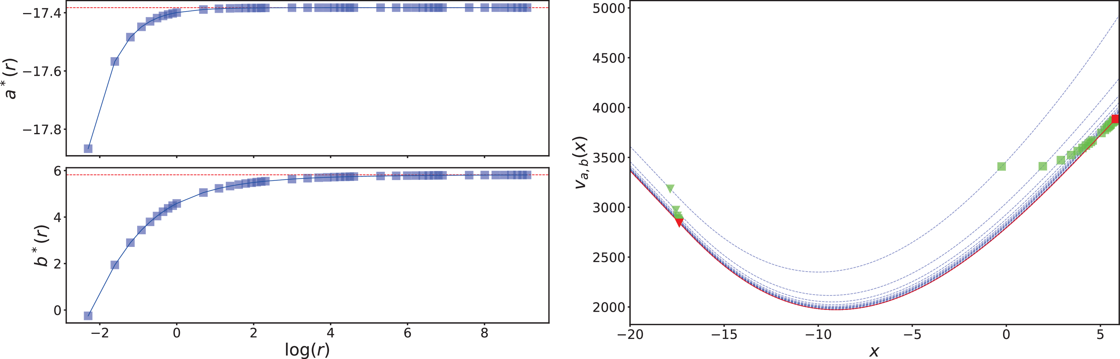
Similarly, the graph on the right in Figure 3 shows the value functions $v_{a^*, b^*}$
corresponding to various r values, alongside the classical value function computed in [Reference Baurdoux and Yamazaki5]. As r increases,
$v_{a^*, b^*}$
corresponding to various r values, alongside the classical value function computed in [Reference Baurdoux and Yamazaki5]. As r increases, $v_{a^*, b^*}$
decreases and converges pointwise to the classical value function.
$v_{a^*, b^*}$
decreases and converges pointwise to the classical value function.
6. Concluding remarks
In this work, we establish the optimality of the periodic–classical barrier strategy under a spectrally negative Lévy model, within a singular control framework where the controller can continuously increase the state process but may only decrease it at independent Poisson arrival times. In this concluding section, we discuss several interesting directions for potential extensions and the associated challenges.
One natural direction for extending the model is to restrict upward control opportunities to the arrival times of an independent Poisson process – either with the same or a different rate parameter – as is currently done for downward control. The main challenge with this extension is that the scale function approach used in this work would likely become unsuitable. When both controls are restricted to random discrete times, the expression for the cost function under a barrier strategy is expected to be substantially more complex and technically involved, thereby complicating the subsequent analysis. Another possible extension is to relax the spectrally one-sided assumption on the Lévy model. This presents a similar challenge, as a general Lévy process does not admit a family of scale functions.
The approach in [Reference Noba and Yamazaki20] may be more suitable for both extensions, as it has been successfully applied to establish the optimality of barrier-type strategies under a general Lévy model for various one-sided control problems. However, unlike this study, where the value function is obtained in a semi-explicit form using scale functions, [Reference Noba and Yamazaki20] does not derive an explicit expression for the value function. Moreover, the method in [Reference Noba and Yamazaki20] has yet to be applied to two-sided control problems, which – based on experience with spectrally one-sided Lévy models – are substantially more challenging than their one-sided counterparts. While we believe that conditions analogous to $\mathfrak{C}$
would play a crucial role in identifying the optimal barrier strategy, establishing the existence of barrier values that satisfy such conditions is expected to require substantial effort. Thus, both extensions pose interesting challenges and are well-suited for future research.
$\mathfrak{C}$
would play a crucial role in identifying the optimal barrier strategy, establishing the existence of barrier values that satisfy such conditions is expected to require substantial effort. Thus, both extensions pose interesting challenges and are well-suited for future research.
Appendix A. Proofs
The following proposition is used for the proofs of Lemmas 4.2 and 4.5.
Proposition A.1. Suppose h is a positive, bounded, measurable function on $\mathbb{R}$
with compact support. We have, for
$\mathbb{R}$
with compact support. We have, for $a \lt b$
and
$a \lt b$
and $x \in \mathbb{R}$
,
$x \in \mathbb{R}$
,
 \begin{align} v_{a, b}^{h}(x) & \;:\!=\; \mathbb{E}_x\bigg[\int^\infty_0{\mathrm{e}}^{-qt}h(Y^{a, b}(t))\,\mathrm{d}t\bigg] \nonumber \\[5pt] & = \frac{\rho_{a, b}^{(q)}(b;\; h) + v_{a, b}^{h}(b)}{Z^{(q)}(b - a)}Z^{(q, r)}_{a, b}(x) - \rho_{a, b}^{(q, r)}(x;\; h) - r\overline{W}^{(q + r)}(x - b)v_{a, b}^{h}(b) \nonumber \\[5pt] & \quad - \int^{x}_b W^{(q + r)}(x - y)h(y)\,\mathrm{d}y, \end{align}
where
 \begin{align} v_{a, b}^{h}(b) & = -\rho_{a, b}^{(q)}(b;\; h) + \bigg(\frac{q}{\Phi_{q+r}}\frac{Z^{(q)}(b-a;\;\Phi_{q+r})}{Z^{(q)}(b-a)}\bigg)^{-1} \nonumber \\[5pt] & \qquad\qquad\qquad\quad \times \bigg({-}\frac{r}{\Phi_{q + r}}\rho_{a, b}^{(q)}(b;\; h) + \int^{\infty}_a h(y) Z^{(q)}(b - y, \Phi_{q + r})\,\mathrm{d}y\bigg). \end{align}
Furthermore, (A.1) and (A.2) also hold for any function $h\colon \mathbb{R} \to \mathbb{R}$
satisfying Assumption 2.1(i), provided that X satisfies Assumption 2.2.
$h\colon \mathbb{R} \to \mathbb{R}$
satisfying Assumption 2.1(i), provided that X satisfies Assumption 2.2.
Proof. The first part of the proposition follows from [Reference Mata, Moreno-Franco, Noba and Pérez17, Proposition 5.1]. For the second part, suppose that h satisfies Assumption 2.1(i) and that X satisfies Assumption 2.2. Let $h^+ \;:\!=\; \max(h, 0)$
and
$h^+ \;:\!=\; \max(h, 0)$
and $h^- \;:\!=\; \max({-}h, 0)$
be the positive and negative parts of h, respectively. The positivity and boundedness assumptions on h can be relaxed through the decomposition
$h^- \;:\!=\; \max({-}h, 0)$
be the positive and negative parts of h, respectively. The positivity and boundedness assumptions on h can be relaxed through the decomposition $h = h^+ - h^-$
and dominated convergence, by noting that
$h = h^+ - h^-$
and dominated convergence, by noting that $\mathbb{E}_x\big[\int^\infty_0{\mathrm{e}}^{-qt}h^+(Y^{a,b}(t))\,\mathrm{d}t\big] \lt \infty$
and
$\mathbb{E}_x\big[\int^\infty_0{\mathrm{e}}^{-qt}h^+(Y^{a,b}(t))\,\mathrm{d}t\big] \lt \infty$
and $\mathbb{E}_x\big[\int^\infty_0{\mathrm{e}}^{-qt}h^-(Y^{a,b}(t))\,\mathrm{d}t\big] \lt \infty$
. Indeed, the finiteness of these expectations holds because h is of at most polynomial growth and
$\mathbb{E}_x\big[\int^\infty_0{\mathrm{e}}^{-qt}h^-(Y^{a,b}(t))\,\mathrm{d}t\big] \lt \infty$
. Indeed, the finiteness of these expectations holds because h is of at most polynomial growth and $a \leq Y^{a,b}(t) \leq Y^{a,\infty}(t)$
, where
$a \leq Y^{a,b}(t) \leq Y^{a,\infty}(t)$
, where $Y^{a, \infty}$
is the classical reflected process from below at a of the spectrally negative Lévy process X, for which it is known that
$Y^{a, \infty}$
is the classical reflected process from below at a of the spectrally negative Lévy process X, for which it is known that $\mathbb{E}_x\big[\int^\infty_0{\mathrm{e}}^{-qt + \theta Y^{a,\infty}(t)}\,\mathrm{d}t\big] \lt \infty$
for any
$\mathbb{E}_x\big[\int^\infty_0{\mathrm{e}}^{-qt + \theta Y^{a,\infty}(t)}\,\mathrm{d}t\big] \lt \infty$
for any $\theta \geq 0$
.
$\theta \geq 0$
.
A.1. Proof of Lemma 4.2
Proof. Proposition A.1 can be applied due to Assumption 2.1(i). With (A.2), via integration by parts as shown in the proof of [Reference Mata, Moreno-Franco, Noba and Pérez17, Lemma 6.3], we obtain
 \begin{equation*} v_{a, b}^{h}(b) = -\rho_{a,b}^{(q)}(b;\; h) + \frac{1}{q}\bigg( h(a) + \int^{\infty}_a h'(y)\frac{Z^{(q)}(b-y,\Phi_{q+r})}{Z^{(q)}(b-a,\Phi_{q+r})}\,\mathrm{d}y\bigg)Z^{(q)}(b-a). \end{equation*}
Substituting this into (A.1) and replacing h with f, we have the desired expression.
A.2. Proof of Lemma 4.3
Proof. Summing the running cost and the control costs, by Lemmas 4.1 and 4.2,
 \begin{align} v_{a,b}(x) & = A\big(Z^{(q, r)}_{a, b}(x) - r\overline{W}^{(q + r)}(x - b)Z^{(q)}(b - a)\big) + B - rC_{\mathrm{D}}\overline{\overline{W}}^{(q + r)}(x - b) \nonumber \\[5pt] & \quad - C_{\mathrm{U}}\bigg(\overline{Z}^{(q, r)}_{a, b}(x) + \frac{\psi'(0+)}{q} - r\overline{W}^{(q + r)}(x - b)\overline{Z}^{(q)}(b - a) \bigg), \quad x \in \mathbb{R}, \end{align}
where
 \begin{align*} A & \;:\!=\; \frac{1}{q}\bigg(f(a) + \int^{\infty}_a f'(y)\frac{Z^{(q)}(b - y, \Phi_{q + r})}{Z^{(q)}(b - a, \Phi_{q + r})}\,\mathrm{d}y + \frac{r}{\Phi_{q + r}}\frac{C_{\mathrm{U}}Z^{(q)}(b - a) + C_{\mathrm{D}}}{Z^{(q)}(b - a, \Phi_{q + r})} + \frac{qC_{\mathrm{U}}}{\Phi_{q + r}}\bigg), \\[5pt] B & \;:\!=\; -\rho_{a, b}^{(q, r)}(x; \;f) + r\overline{W}^{(q + r)}(x - b)\rho_{a, b}^{(q)}(b;\; f) - \int^{x}_b f(y) W^{(q + r)}(x - y)\, \mathrm{d} y. \end{align*}
First, we simplify the expression for A.
Lemma A.1. For $a\lt b$
,
$a\lt b$
,
 $$ \int^\infty_a Z^{(q)}(b - y, \Phi_{q + r})\,\mathrm{d}y = (Z^{(q)}(b - a, \Phi_{q + r}) + r\overline{W}^{(q)}(b - a)) / \Phi_{q+r}. $$
Proof. By exchanging the order of integration and the second equality of (4.2),
 \begin{align*} \int^b_a Z^{(q)}(b - y, \Phi_{q + r})\, \mathrm{d} y & = r\int^b_a\int_0^{\infty}{\mathrm{e}}^{-\Phi_{q + r} z} W^{(q)}(z + b - y)\, \mathrm{d} z \, \mathrm{d} y \\[5pt] & = r\int_0^{\infty}{\mathrm{e}}^{-\Phi_{q + r} z} \int^b_a W^{(q)}(z + b - y)\,\mathrm{d} y\,\mathrm{d} z \\[5pt] & = r\int_0^{\infty}{\mathrm{e}}^{-\Phi_{q + r} z}\left(\overline{W}^{(q)}(z + b - a) - \overline{W}^{(q)}(z)\right)\,\mathrm{d} z. \end{align*}
By integration by parts and the second equality of (4.2),
 \begin{equation*} \int_0^{\infty}{\mathrm{e}}^{-\Phi_{q + r} z} \overline{W}^{(q)}(z + b - a)\,\mathrm{d} z = \frac{1}{\Phi_{q + r}}\overline{W}^{(q)}(b - a) + \frac{1}{r\Phi_{q+r}} Z^{(q)}(b - a, \Phi_{q + r}) . \end{equation*}
In particular, $\int_0^{\infty}{\mathrm{e}}^{-\Phi_{q + r} z} \overline{W}^{(q)}(z)\,\mathrm{d}z = (r\Phi_{q + r})^{-1} Z^{(q)}(0, \Phi_{q + r}) = (r\Phi_{q + r})^{-1}$
. Thus,
$\int_0^{\infty}{\mathrm{e}}^{-\Phi_{q + r} z} \overline{W}^{(q)}(z)\,\mathrm{d}z = (r\Phi_{q + r})^{-1} Z^{(q)}(0, \Phi_{q + r}) = (r\Phi_{q + r})^{-1}$
. Thus,
 \begin{equation*} \int^b_a Z^{(q)}(b - y, \Phi_{q + r})\, \mathrm{d} y = \frac{1}{\Phi_{q+r}}\big(Z^{(q)}(b - a, \Phi_{q + r}) + r\overline{W}^{(q)}(b - a) - 1\big). \end{equation*}
In addition, $\int^\infty_b Z^{(q)}(b - y, \Phi_{q + r})\, \mathrm{d} y = \int^\infty_b{\mathrm{e}}^{\Phi_{q+r}(b - y)}\, \mathrm{d} y = \int^\infty_0{\mathrm{e}}^{-\Phi_{q + r}y}\, \mathrm{d} y = (\Phi_{q + r})^{-1}$
. By summing these terms, the claim follows.
$\int^\infty_b Z^{(q)}(b - y, \Phi_{q + r})\, \mathrm{d} y = \int^\infty_b{\mathrm{e}}^{\Phi_{q+r}(b - y)}\, \mathrm{d} y = \int^\infty_0{\mathrm{e}}^{-\Phi_{q + r}y}\, \mathrm{d} y = (\Phi_{q + r})^{-1}$
. By summing these terms, the claim follows.
By Lemma A.1,
 \begin{align*} \int^{\infty}_a f'(y) Z^{(q)}(b - y, \Phi_{q + r})\, \mathrm{d} y & = \int^{\infty}_a \tilde{f}'(y) Z^{(q)}(b - y, \Phi_{q + r})\, \mathrm{d} y \\[5pt] & \quad - \frac{qC_{\mathrm{U}}}{\Phi_{q+r}}\big(Z^{(q)}(b - a, \Phi_{q + r}) + r\overline{W}^{(q)}(b - a)\big). \end{align*}
Substituting this into the expression for A, we have
 \begin{equation} A = \frac{1}{q}\bigg(f(a) + \frac{\Gamma(a, b)}{Z^{(q)}(b - a, \Phi_{q + r})}\bigg). \end{equation}
Second, we write B in terms of $\tilde{f}\colon x \mapsto f(x) + qC_{\mathrm{U}}x$
, for
$\tilde{f}\colon x \mapsto f(x) + qC_{\mathrm{U}}x$
, for $x \in \mathbb{R}$
. We have
$x \in \mathbb{R}$
. We have
 \begin{equation} \rho_{a, b}^{(q)}(x;\; f) = \rho_{a, b}^{(q)}(x;\; \tilde{f}) - qC_{\mathrm{U}} \rho_{a, b}^{(q)}(x;\; y \mapsto y), \end{equation}
where, due to integration by parts,
 \begin{equation} \rho_{a, b}^{(q)}(x;\; y \mapsto y) = \overline{W}^{(q)}(x - a) a - \overline{W}^{(q)}(x - b) b + \overline{\overline{W}}^{(q)}(x - a) - \overline{\overline{W}}^{(q)}(x - b). \end{equation}
In particular, at $x = b$
,
$x = b$
,
 \begin{equation} \rho_{a, b}^{(q)}(b;\; y \mapsto y) = \overline{W}^{(q)}(b - a) a + \overline{\overline{W}}^{(q)}(b - a). \end{equation}
More generally, we have
 \begin{equation} \rho_{a, b}^{(q, r)}(x;\; f) = \rho_{a, b}^{(q, r)}(x;\; \tilde{f}) - q C_{\mathrm{U}} \rho_{a, b}^{(q, r)}(x;\; y \mapsto y), \end{equation}
where $\rho_{a, b}^{(q, r)}(x;\; y \mapsto y) = \rho_{a, b}^{(q)}(x;\; y \mapsto y) + r\int^{x}_b W^{(q + r)}(x - y)\rho_{a, b}^{(q)}(y;\; z \mapsto z)\, \mathrm{d} y$
.
$\rho_{a, b}^{(q, r)}(x;\; y \mapsto y) = \rho_{a, b}^{(q)}(x;\; y \mapsto y) + r\int^{x}_b W^{(q + r)}(x - y)\rho_{a, b}^{(q)}(y;\; z \mapsto z)\, \mathrm{d} y$
.
Applying integration by parts twice, we obtain
 \begin{align} \int^{x}_b f(y) W^{(q + r)}(x - y)\, \mathrm{d} y & = \int^{x}_b \tilde{f}'(y) \overline{W}^{(q + r)}(x - y)\, \mathrm{d} y \nonumber \\[5pt] & \quad + f(b)\overline{W}^{(q + r)}(x - b) - qC_{\mathrm{U}}\overline{\overline{W}}^{(q + r)}(x - b). \end{align}
Substituting (A.5), (A.8), and (A.9) into the expression for B, for $x \in \mathbb{R}$
,
$x \in \mathbb{R}$
,
 \begin{align} B & = -\rho_{a, b}^{(q, r)}(x;\; \tilde{f}) + qC_{\mathrm{U}}\rho_{a, b}^{(q, r)}(x;\; y \mapsto y) + r\overline{W}^{(q + r)}(x - b) \rho_{a, b}^{(q)}(b;\; \tilde{f}) \nonumber \\[5pt] & \quad - r\overline{W}^{(q + r)}(x - b) qC_{\mathrm{U}} \rho_{a, b}^{(q)}(b;\; y \mapsto y) - \int^{x}_b \tilde{f}'(y) \overline{W}^{(q + r)}(x - y)\, \mathrm{d} y \nonumber \\[5pt] & \quad - f(b)\overline{W}^{(q + r)}(x - b) + qC_{\mathrm{U}}\overline{\overline{W}}^{(q + r)}(x - b). \end{align}
With
 \begin{align*} \overline{W}^{(q, r)}_{a, b}(x) & \;:\!=\; \overline{W}^{(q)}(x - a) + r\int^x_b W^{(q + r)}(x - y)\overline{W}^{(q)}(y - a)\, \mathrm{d} y, \\[5pt] \overline{\overline{W}}^{(q, r)}_{a, b}(x) & \;:\!=\; \overline{\overline{W}}^{(q)}(x - a) + r\int^x_b W^{(q + r)}(x - y)\overline{\overline{W}}^{(q)}(y - a)\, \mathrm{d} y, \end{align*}
and using (A.6), we have
 \begin{equation*} \rho_{a, b}^{(q, r)}(x;\; y \mapsto y) = a\overline{W}^{(q, r)}_{a, b}(x) + \overline{\overline{W}}^{(q, r)}_{a, b}(x) - b\overline{W}^{(q, r)}_{b, b}(x) - \overline{\overline{W}}^{(q, r)}_{b, b}(x). \end{equation*}
In terms of (4.6) and (4.7), we can write
 \begin{align*} \overline{W}^{(q, r)}_{a, b}(x) & = \frac{1}{q} \Big( Z^{(q, r)}_{a, b}(x) - 1 - r\overline{W}^{(q + r)}(x - b) \Big), \\[5pt] \overline{\overline{W}}^{(q, r)}_{a, b}(x) & = \frac{1}{q}\Big(\overline{Z}^{(q, r)}_{a, b}(x) - (x - a) - r\overline{W}^{(q + r)}(x - b)(b - a) - r\overline{\overline{W}}^{(q + r)}(x - b)\Big). \end{align*}
Moreover, by [Reference Loeffen, Renaud and Zhou16, (6)], we can write $\overline{W}^{(q, r)}_{b, b}(x) = \overline{W}^{(q + r)}(x - b)$
. Then, by noticing that
$\overline{W}^{(q, r)}_{b, b}(x) = \overline{W}^{(q + r)}(x - b)$
. Then, by noticing that $\overline{\overline{W}}^{(q, r)}_{b, b}$
is an anti-derivative of
$\overline{\overline{W}}^{(q, r)}_{b, b}$
is an anti-derivative of $\overline{W}^{(q, r)}_{b, b}$
and using the identity
$\overline{W}^{(q, r)}_{b, b}$
and using the identity $\overline{W}^{(q, r)}_{b, b}(x) = \overline{W}^{(q + r)}(x - b)$
, we obtain
$\overline{W}^{(q, r)}_{b, b}(x) = \overline{W}^{(q + r)}(x - b)$
, we obtain $\overline{\overline{W}}^{(q, r)}_{b, b}(x) = \overline{\overline{W}}^{(q + r)}(x - b)$
. Substituting these,
$\overline{\overline{W}}^{(q, r)}_{b, b}(x) = \overline{\overline{W}}^{(q + r)}(x - b)$
. Substituting these,
 \begin{align} \rho_{a, b}^{(q, r)}(x;\; y \mapsto y) & = \frac 1 q \Big(a Z^{(q, r)}_{a, b}(x) + \overline{Z}^{(q, r)}_{a, b}(x) - x - r\overline{W}^{(q + r)}(x - b)b - r\overline{\overline{W}}^{(q + r)}(x - b) \Big) \nonumber \\[5pt]& \quad - \overline{\overline{W}}^{(q + r)}(x - b) - \overline{W}^{(q + r)}(x - b)b. \end{align}
Substituting (A.7) and (A.11) in (A.10),
 \begin{align*} B & = -\rho_{a, b}^{(q, r)}(x;\; \tilde{f}) + C_{\mathrm{U}}\Big(aZ^{(q, r)}_{a, b}(x) + \overline{Z}^{(q, r)}_{a, b}(x) - x - r\overline{W}^{(q + r)}(x - b)b - r\overline{\overline{W}}^{(q + r)}(x - b)\Big) \\[5pt]& \quad + r\overline{W}^{(q + r)}(x - b)\rho_{a, b}^{(q)}(b;\; \tilde{f}) - r\overline{W}^{(q + r)}(x - b)qC_{\mathrm{U}}\Big(\overline{W}^{(q)}(b - a) a + \overline{\overline{W}}^{(q)}(b - a) \Big) \\[5pt]& \quad - \int^{x}_b \tilde{f}'(y) \overline{W}^{(q + r)}(x - y)\, \mathrm{d} y - \tilde{f}(b)\overline{W}^{(q + r)}(x - b). \end{align*}
Finally, substituting this expression for B and (A.4) into (A.3), and simplifying, we obtain the desired expression.
A.3. Proof of Lemma 4.4
Proof. By direct computation and the smoothness of the scale functions, we obtain the following results for $x \in \mathbb{R}\backslash \{a, b\}$
and for any continuous and almost everywhere differentiable function
$x \in \mathbb{R}\backslash \{a, b\}$
and for any continuous and almost everywhere differentiable function $h\colon \mathbb{R} \to \mathbb{R}$
:
$h\colon \mathbb{R} \to \mathbb{R}$
:
 \begin{align} \frac{\mathrm{d}}{\mathrm{d}x} Z^{(q, r)}_{a, b}(x) & = qW^{(q, r)}_{a, b}(x) + rW^{(q + r)}(x - b) Z^{(q)}(b - a), \\[-12pt] \nonumber \end{align}
 \begin{align} \frac{\mathrm{d}}{\mathrm{d}x}\rho_{a, b}^{(q)}(x;\; h) & = -W^{(q)}(x - b)h(b) + W^{(q)}(x - a)h(a) + \int^{b}_a W^{(q)}(x - y)h'(y)\,\mathrm{d} y. \\[0pt] \nonumber \end{align}
We further compute $({\mathrm{d}}/{\mathrm{d}x})\rho_{a, b}^{(q, r)}(x;\; h)$
. Recalling (4.4), by partial integration,
$({\mathrm{d}}/{\mathrm{d}x})\rho_{a, b}^{(q, r)}(x;\; h)$
. Recalling (4.4), by partial integration,
 \begin{equation} \frac{\mathrm{d}}{\mathrm{d}x}\rho_{a, b}^{(q, r)}(x;\; h) = \frac{\mathrm{d}}{\mathrm{d}x}\rho_{a, b}^{(q)}(x;\; h) + rW^{(q + r)}(x - b)\rho_{a, b}^{(q)}(b;\; h) + C, \quad x\in \mathbb{R}\backslash\{a, b\}, \end{equation}
where, by (A.13) and [Reference Loeffen, Renaud and Zhou16, (6)],
 \begin{align*} C & \;:\!=\; r\int^{x}_{b} W^{(q + r)}(x - y)\frac{\mathrm{d}}{\mathrm{d}y}\rho_{a, b}^{(q)}(y;\; h)\,\mathrm{d}y \\[5pt] & = -h(b)(W^{(q + r)}(x - b) - W^{(q)}(x - b)) + rh(a)\int^{x}_{b} W^{(q + r)}(x - y)W^{(q)}(y - a)\,\mathrm{d}y \\[5pt] & \quad + r\int^{x}_{b} W^{(q + r)}(x - y) \int^{b}_a W^{(q)}(y - z)h'(z)\, \mathrm{d} z\, \mathrm{d} y. \end{align*}
Substituting this in (A.14) and using (4.5), for $x\in \mathbb{R}\backslash\{a, b\}$
,
$x\in \mathbb{R}\backslash\{a, b\}$
,
 \begin{align} \frac{\mathrm{d}}{\mathrm{d}x}\rho_{a, b}^{(q, r)}(x;\; h) & = h(a)W^{(q, r)}_{a, b}(x) + rW^{(q + r)}(x - b)\rho_{a, b}^{(q)}(b;\; h) \nonumber \\[5pt] & \quad - h(b)W^{(q + r)}(x - b) + \rho_{a, b}^{(q, r)}(x;\; h'). \end{align}
We obtain (4.12) by differentiating (4.10) using (A.12) and (A.15). The statement that (4.12) is defined on $\mathbb{R}\backslash \{a\}$
can be confirmed by inspecting its left- and right-hand limits and using the smoothness of scale functions. To obtain the second derivative of
$\mathbb{R}\backslash \{a\}$
can be confirmed by inspecting its left- and right-hand limits and using the smoothness of scale functions. To obtain the second derivative of $v_{a, b}$
, we directly differentiate (4.12). This gives (4.13), which is again defined on
$v_{a, b}$
, we directly differentiate (4.12). This gives (4.13), which is again defined on $\mathbb{R}\backslash \{a\}$
by the smoothness of scale functions.
$\mathbb{R}\backslash \{a\}$
by the smoothness of scale functions.
A.4. Proof of Lemma 4.5
Proof. By (4.3) and the definition of $\tilde{f}$
, for
$\tilde{f}$
, for $x \in \mathbb{R}$
,
$x \in \mathbb{R}$
,
 \begin{equation*} \rho_{a, b}^{(q, r)}(x;\; f') = \rho_{a, b}^{(q,r)}(x;\; \tilde{f}') - q C_{\mathrm{U}} \rho_{a, b}^{(q,r)}(x;\; 1), \end{equation*}
where, with $\rho_{a, b}^{(q)}(x;\; 1) = \int^{b}_a W^{(q)}(x - y) \, \mathrm{d} y = (Z^{(q)}(x - a) - Z^{(q)}(x - b))/q$
, we can write
$\rho_{a, b}^{(q)}(x;\; 1) = \int^{b}_a W^{(q)}(x - y) \, \mathrm{d} y = (Z^{(q)}(x - a) - Z^{(q)}(x - b))/q$
, we can write
 \begin{equation*} \rho_{a, b}^{(q,r)}(x;\; 1) = \rho_{a, b}^{(q)}(x;\; 1) + r\int^{x}_b W^{(q + r)}(x - y)\rho_{a, b}^{(q)}(y;\; 1) \mathrm{d} y = \frac{1}{q} \Big(Z^{(q, r)}_{a, b}(x) - Z^{(q, r)}_{b, b}(x)\Big). \end{equation*}
Using [Reference Loeffen, Renaud and Zhou16, (6)], we obtain $Z^{(q, r)}_{b, b}(x) = Z^{(q + r)}(x - b)$
, and thus
$Z^{(q, r)}_{b, b}(x) = Z^{(q + r)}(x - b)$
, and thus
 \begin{equation} \rho_{a, b}^{(q, r)}(x;\; f') = \rho_{a, b}^{(q, r)}(x;\; \tilde{f}') - C_{\mathrm{U}}\Big(Z^{(q, r)}_{a, b}(x) - Z^{(q + r)}(x - b)\Big). \end{equation}
Moreover, for $x \in \mathbb{R}$
, we have
$x \in \mathbb{R}$
, we have
 \begin{equation} \int^{x}_{b} W^{(q + r)}(x - y)f'(y)\, \mathrm{d} y = \int^{x}_{b} W^{(q + r)}(x - y)\tilde{f}'(y)\, \mathrm{d} y - qC_{\mathrm{U}}\overline{W}^{(q + r)}(x - b). \end{equation}
Rewriting (A.2) with $h = f'$
by applying Lemma A.1 and (A.16), and simplifying using (4.14), we obtain
$h = f'$
by applying Lemma A.1 and (A.16), and simplifying using (4.14), we obtain
 \begin{align} v_{a, b}^{f'}(b) & = -\rho_{a, b}^{(q)}(b;\; \tilde{f}') + qC_{\mathrm{U}}\overline{W}^{(q)}(b - a) \nonumber \\[5pt] & \quad + \bigg(\frac{q}{\Phi_{q + r}} \frac{Z^{(q)}(b - a;\; \Phi_{q + r})}{Z^{(q)}(b - a)}\bigg)^{-1} \nonumber \\[5pt] & \qquad \times \bigg({-}\frac{r}{\Phi_{q + r}}\rho_{a, b}^{(q)}(b;\; \tilde{f}') + \int^{\infty}_a \tilde{f}'(y) Z^{(q)}(b - y, \Phi_{q + r})\, \mathrm{d} y \nonumber \\[5pt] & \qquad\qquad - \frac{qC_{\mathrm{U}}}{\Phi_{q + r}} Z^{(q)}(b - a, \Phi_{q + r})\bigg) \nonumber \\[5pt] & = -\rho_{a, b}^{(q)}(b;\; \tilde{f}') - C_{\mathrm{U}} + \frac{Z^{(q)}(b - a)}{qZ^{(q)}(b - a;\; \Phi_{q + r})}\gamma(a, b). \end{align}
Substituting (A.16), (A.17), and (A.18) into (A.1) with $h = f'$
, and simplifying, we obtain the desired result.
$h = f'$
, and simplifying, we obtain the desired result.
A.5. Proof of Lemma 4.6
Proof. As $b \mapsto \Gamma(a, b)$
is continuous on
$b \mapsto \Gamma(a, b)$
is continuous on $(a, \infty)$
, the first claim holds by setting
$(a, \infty)$
, the first claim holds by setting $b = a+$
in (4.11) and noting that
$b = a+$
in (4.11) and noting that $Z^{(q)}(a - y, \Phi_{q + r}) = \exp(\Phi_{q + r}(a - y))$
for
$Z^{(q)}(a - y, \Phi_{q + r}) = \exp(\Phi_{q + r}(a - y))$
for $y \gt a$
.
$y \gt a$
.
For the second claim, by the second equality of (4.2) we have two bounds for $Z^{(q)}(\cdot, \Phi_{q + r})$
. First, with
$Z^{(q)}(\cdot, \Phi_{q + r})$
. First, with $W_{\Phi_{q}}(x) = {\mathrm{e}}^{-\Phi_q x}W^{(q)}(x)$
(see [Reference Kyprianou12, p. 247]), for
$W_{\Phi_{q}}(x) = {\mathrm{e}}^{-\Phi_q x}W^{(q)}(x)$
(see [Reference Kyprianou12, p. 247]), for $x \in \mathbb{R}$
,
$x \in \mathbb{R}$
,
 \begin{equation*} Z^{(q)}(x, \Phi_{q + r}) = r\int^\infty_0{\mathrm{e}}^{-\Phi_{q + r} y}W^{(q)}(x + y)\, \mathrm{d} y = r{\mathrm{e}}^{\Phi_{q} x}\int^\infty_0{\mathrm{e}}^{-(\Phi_{q + r} - \Phi_{q}) y}W_{\Phi_{q}}(x + y)\, \mathrm{d} y. \end{equation*}
Since $W_{\Phi_q}$
is increasing,
$W_{\Phi_q}$
is increasing,
 $$ \frac{r{\mathrm{e}}^{\Phi_{q} x} W_{\Phi_{q}}(x)}{\Phi_{q + r} - \Phi_{q}} \leq Z^{(q)}(x, \Phi_{q + r}) \leq \frac{r{\mathrm{e}}^{\Phi_{q} x} W_{\Phi_{q}}(\infty)}{\Phi_{q + r} - \Phi_{q}}, $$
where $W_{\Phi_{q}}(\infty) \;:\!=\; \lim_{x \to \infty} W_{\Phi_{q}}(x)$
is well-defined and finite. Thus, for
$W_{\Phi_{q}}(\infty) \;:\!=\; \lim_{x \to \infty} W_{\Phi_{q}}(x)$
is well-defined and finite. Thus, for $b \gt b'$
with
$b \gt b'$
with $b' \gt a$
fixed,
$b' \gt a$
fixed,
 \begin{align*} \bigg|\tilde{f}'(z)\frac{Z^{(q)}(b-z,\Phi_{q+r})}{Z^{(q)}(b-a,\Phi_{q+r})}\mathbf{1}_{\{a\leq z\}}\bigg| & \leq |\tilde{f}'(z)|\frac{{\mathrm{e}}^{\Phi_q(b - z)} W_{\Phi_{q}}(\infty)}{{\mathrm{e}}^{\Phi_q (b - a)} W_{\Phi_{q}}(b - a)} \\[5pt] & \leq |\tilde{f}'(z)|{\mathrm{e}}^{-\Phi_q (z - a)}\frac{ W_{\Phi_{q}}(\infty)}{W_{\Phi_{q}}(b' - a)}, \end{align*}
which is integrable. Thus, dominated convergence gives
 \begin{equation*} \lim_{b \to \infty} \frac{\Gamma(a, b)}{Z^{(q)}(b - a, \Phi_{q + r})} = \int^{\infty}_0{\mathrm{e}}^{-\Phi_q z} \tilde{f}'(z + a)\, \mathrm{d} z. \end{equation*}
A.6. Proof of Lemma 4.7
Proof. For (i), by (4.21) and the definition of $\overline{a}$
, we have
$\overline{a}$
, we have $\Gamma(\bar{a}, \bar{a}+) \gt 0$
. From (4.11), it is easy to see that
$\Gamma(\bar{a}, \bar{a}+) \gt 0$
. From (4.11), it is easy to see that $b \mapsto \Gamma(\bar{a}, b)$
is strictly increasing on
$b \mapsto \Gamma(\bar{a}, b)$
is strictly increasing on $(\bar{a}, \infty)$
. Hence,
$(\bar{a}, \infty)$
. Hence, $\underline{\Gamma}(\bar{a}) \gt 0$
.
$\underline{\Gamma}(\bar{a}) \gt 0$
.
For (ii), we show separately that $\underline{\Gamma}(\underline{a}_1 \vee \underline{a}_2) \lt 0$
, first for the case
$\underline{\Gamma}(\underline{a}_1 \vee \underline{a}_2) \lt 0$
, first for the case $\underline{a}_2 \geq \underline{a}_1$
, and then for the case
$\underline{a}_2 \geq \underline{a}_1$
, and then for the case $\underline{a}_2 \lt \underline{a}_1$
.
$\underline{a}_2 \lt \underline{a}_1$
.
Suppose that $\underline{a}_2 \geq \underline{a}_1$
. By (4.16) with
$\underline{a}_2 \geq \underline{a}_1$
. By (4.16) with $a = \underline{a}_2$
and (4.24), we have, for any
$a = \underline{a}_2$
and (4.24), we have, for any $b \gt \underline{a}_2$
,
$b \gt \underline{a}_2$
,
 \begin{align*} \frac{\gamma(\underline{a}_2, b)}{qZ^{(q)}(b - \underline{a}_2;\; \Phi_{q + r})} - C_{\mathrm{U}} & = \mathbb{E}_{\underline{a}_2}\bigg[\int^\infty_0{\mathrm{e}}^{-qt} f'(Y^{\underline{a}_2, b}(t))\, \mathrm{d} t\bigg] \\[5pt] & \lt \mathbb{E}_{\underline{a}_2}\bigg[\int^\infty_0{\mathrm{e}}^{-qt} f'(Y^{\underline{a}_2, \infty}(t))\, \mathrm{d} t\bigg] = -C_{\mathrm{U}}, \end{align*}
where the inequality holds because $Y^{\underline{a}_2, b}(t) \leq Y^{\underline{a}_2, \infty}(t)$
for all
$Y^{\underline{a}_2, b}(t) \leq Y^{\underline{a}_2, \infty}(t)$
for all $t \geq 0$
. To see why the inequality is strict, first note that
$t \geq 0$
. To see why the inequality is strict, first note that $\underline{a}_2 \lt \bar{a} \lt \bar{\bar{a}}$
implies the existence of some
$\underline{a}_2 \lt \bar{a} \lt \bar{\bar{a}}$
implies the existence of some $c \gt \underline{a}_2$
and
$c \gt \underline{a}_2$
and $\varepsilon \gt 0$
such that
$\varepsilon \gt 0$
such that $f'(c) \lt f'(c + \varepsilon)$
. Moreover, since the set
$f'(c) \lt f'(c + \varepsilon)$
. Moreover, since the set $\{t \in [0,\infty)\colon Y^{\underline{a}_2, b}(t) \lt c,\,Y^{\underline{a}_2, \infty}(t) \gt c + \varepsilon\}$
has a positive Lebesgue measure with positive probability, the inequality is indeed strict. This inequality implies
$\{t \in [0,\infty)\colon Y^{\underline{a}_2, b}(t) \lt c,\,Y^{\underline{a}_2, \infty}(t) \gt c + \varepsilon\}$
has a positive Lebesgue measure with positive probability, the inequality is indeed strict. This inequality implies
 \begin{equation} 0 \gt \gamma(\underline{a}_2, b) = \Phi_{q+r} \Gamma(\underline{a}_2, b) - r\big(C_{\mathrm{U}} + C_{\mathrm{D}} + \rho_{\underline{a}_2, b}^{(q)}(b;\; \tilde{f}')\big), \quad b \gt \underline{a}_2. \end{equation}
Now, since f
′ is non-decreasing and $f'(\infty) \gt qC_{\mathrm{D}}$
by Assumption 2.1(iii), for some sufficiently large
$f'(\infty) \gt qC_{\mathrm{D}}$
by Assumption 2.1(iii), for some sufficiently large $\tilde{b}$
,
$\tilde{b}$
,
 \begin{align*} C_{\mathrm{D}} \lt \mathbb{E}_{\tilde{b}}\bigg[\int^\infty_0{\mathrm{e}}^{-qt}f'(Y^{\underline{a}_2,\tilde{b}}(t))\,\mathrm{d}t\bigg] & = v^{f'}_{\underline{a}_2, \tilde{b}}(\tilde{b}) \\[5pt] & = \frac{Z^{(q)}(\tilde{b} - \underline{a}_2)}{qZ^{(q)}(\tilde{b} - \underline{a}_2;\; \Phi_{q + r})} \gamma(\underline{a}_2, \tilde{b}) - \rho_{\underline{a}_2, \tilde{b}}^{(q)}(\tilde{b};\; \tilde{f}') - C_{\mathrm{U}}, \end{align*}
where we used (4.17) for the last equality. This, together with (A.19) with $b = \tilde{b}$
, gives
$b = \tilde{b}$
, gives $\rho_{\underline{a}_2, \tilde{b}}^{(q)}(\tilde{b};\; \tilde{f}') + C_{\mathrm{U}} + C_{\mathrm{D}} \lt 0$
. Substituting this inequality back into (A.19), we have
$\rho_{\underline{a}_2, \tilde{b}}^{(q)}(\tilde{b};\; \tilde{f}') + C_{\mathrm{U}} + C_{\mathrm{D}} \lt 0$
. Substituting this inequality back into (A.19), we have $\Gamma(\underline{a}_2, \tilde{b}) \lt 0$
, and therefore
$\Gamma(\underline{a}_2, \tilde{b}) \lt 0$
, and therefore $\underline{\Gamma}(\underline{a}_1 \vee \underline{a}_2) = \underline{\Gamma}(\underline{a}_2) \leq \Gamma(\underline{a}_2, \tilde{b}) \lt 0$
.
$\underline{\Gamma}(\underline{a}_1 \vee \underline{a}_2) = \underline{\Gamma}(\underline{a}_2) \leq \Gamma(\underline{a}_2, \tilde{b}) \lt 0$
.
Now suppose that $\underline{a}_1 \gt \underline{a}_2$
. By (4.14) and the definition of
$\underline{a}_1 \gt \underline{a}_2$
. By (4.14) and the definition of $\underline{a}_1$
, we have
$\underline{a}_1$
, we have $\gamma(\underline{a}_1, \underline{a}_1+) = - r(C_{\mathrm{U}} + C_{\mathrm{D}}) \lt 0$
. Since
$\gamma(\underline{a}_1, \underline{a}_1+) = - r(C_{\mathrm{U}} + C_{\mathrm{D}}) \lt 0$
. Since $\gamma(\underline{a}_1, \cdot)$
is the partial derivative of
$\gamma(\underline{a}_1, \cdot)$
is the partial derivative of $\Gamma(\underline{a}_1, \cdot)$
, which starts at
$\Gamma(\underline{a}_1, \cdot)$
, which starts at $\Gamma(\underline{a}_1,\underline{a}_1+) = 0$
, the function
$\Gamma(\underline{a}_1,\underline{a}_1+) = 0$
, the function $\Gamma(\underline{a}_1, \cdot)$
must go below zero. Thus,
$\Gamma(\underline{a}_1, \cdot)$
must go below zero. Thus, $0 \gt \underline{\Gamma}(\underline{a}_1) = \underline{\Gamma}(\underline{a}_1 \vee \underline{a}_2)$
.
$0 \gt \underline{\Gamma}(\underline{a}_1) = \underline{\Gamma}(\underline{a}_1 \vee \underline{a}_2)$
.
A.7. Proof of Lemma 4.8
Proof. By taking the partial derivative of $\Gamma$
with respect to a, we obtain, for almost every a at which
$\Gamma$
with respect to a, we obtain, for almost every a at which $\tilde{f}'(a)$
exists,
$\tilde{f}'(a)$
exists, $({\partial}/{\partial a})\Gamma(a, b) = - \tilde{f}'(a)Z^{(q)}(b - a, \Phi_{q + r})$
,
$({\partial}/{\partial a})\Gamma(a, b) = - \tilde{f}'(a)Z^{(q)}(b - a, \Phi_{q + r})$
, $a \lt b$
, which is positive for
$a \lt b$
, which is positive for $a \lt \bar{a}$
. For
$a \lt \bar{a}$
. For $a' \lt a \leq \bar{a}$
, notice that
$a' \lt a \leq \bar{a}$
, notice that
 \begin{align*} \underline{\Gamma}(a') & \leq \inf_{b \gt a} \Gamma(a', b) \\[5pt] & = \inf_{b\gt a}\bigg(\Gamma(a,b) + \int^a_{a'}\tilde{f}'(y)Z^{(q)}(b-y,\Phi_{q+r})\,\mathrm{d}y\bigg) \\[5pt] & \leq \inf_{b\gt a}\bigg(\Gamma(a,b) + \int^{(a+a')/2}_{a'}\tilde{f}'(y)Z^{(q)}(b-y,\Phi_{q+r})\,\mathrm{d}y\bigg) \end{align*}
 \begin{align*} & \leq \inf_{b \gt a}\bigg(\Gamma(a, b) + Z^{(q)}\bigg(b - \frac{a + a'}{2}, \Phi_{q + r}\bigg)\int^{(a + a')/2}_{a'} \tilde{f}'(y)\, \mathrm{d} y\bigg) \\[5pt] & \leq \underline{\Gamma}(a) + Z^{(q)}\bigg(\frac{a - a'}{2}, \Phi_{q + r}\bigg) \int^{(a + a')/2}_{a'} \tilde{f}'(y)\, \mathrm{d} y \lt \underline{\Gamma}(a). \end{align*}
Hence, $a \mapsto \underline{\Gamma}(a)$
is strictly increasing on
$a \mapsto \underline{\Gamma}(a)$
is strictly increasing on $({-}\infty, \bar{a})$
. Continuity is guaranteed because
$({-}\infty, \bar{a})$
. Continuity is guaranteed because $\Gamma(a, b) \xrightarrow{b \uparrow \infty} \infty$
for all
$\Gamma(a, b) \xrightarrow{b \uparrow \infty} \infty$
for all $a \gt \underline{a}_2$
, by (4.22) and the definition of
$a \gt \underline{a}_2$
, by (4.22) and the definition of $\underline{a}_2$
as in (4.23).
$\underline{a}_2$
as in (4.23).
A.8. Proof of Lemma 4.9
Proof. Fix an admissible strategy $\pi \in \Pi$
. For a càdlàg process A, denote its jump at time s by
$\pi \in \Pi$
. For a càdlàg process A, denote its jump at time s by $\Delta A(s) \;:\!=\; A(s) - A(s{-})$
and its continuous part by
$\Delta A(s) \;:\!=\; A(s) - A(s{-})$
and its continuous part by $A^{\mathrm{c}}$
, such that
$A^{\mathrm{c}}$
, such that $A(s) = A^{\mathrm{c}}(s) + \sum_{0 \leq u \leq s}\Delta A(u)$
. By first applying Itô’s lemma and then rearranging terms, we obtain
$A(s) = A^{\mathrm{c}}(s) + \sum_{0 \leq u \leq s}\Delta A(u)$
. By first applying Itô’s lemma and then rearranging terms, we obtain
 \begin{align*} w(x) & = -\int^{t \wedge \tau_n}_0{\mathrm{e}}^{-qs} (\mathcal{L}-q) w(Y^\pi(s{-}))\, \mathrm{d} s \\[5pt] & \quad - \int_{[0, t \wedge \tau_n]}{\mathrm{e}}^{-qs}w'(Y^\pi(s{-}))\, \mathrm{d} R^{\pi,c}(s) + C_{\mathrm{D}} \int_{[0, t \wedge \tau_n]}{\mathrm{e}}^{-qs} \nu^\pi(s)\, \mathrm{d} N_r(s) \\[5pt]& \quad - \int^{t \wedge \tau_n}_0 r{\mathrm{e}}^{-qs} [C_{\mathrm{D}} \nu^\pi(s) + w(Y^\pi(s{-}) - \nu^\pi(s)) - w(Y^\pi(s{-}))]\, \mathrm{d} s \\[5pt]& \quad - \sum_{0\leq s \leq t \wedge \tau_n}{\mathrm{e}}^{-qs}[w(Y^\pi(s{-}) + \Delta X(s) + \Delta R^\pi(s)) - w(Y^\pi(s{-}) + \Delta X(s))] \\[5pt]& \quad - M(t \wedge \tau_n) + {\mathrm{e}}^{-q(t\wedge \tau_n)} w(Y^\pi(t\wedge \tau_n)), \end{align*}
where $(M(t \wedge \tau_n);\; t \geq 0)$
is defined in [Reference Pérez and Yamazaki21, (A.1)]. Noting that
$(M(t \wedge \tau_n);\; t \geq 0)$
is defined in [Reference Pérez and Yamazaki21, (A.1)]. Noting that $Y^\pi(s{-})$
is bounded almost surely on
$Y^\pi(s{-})$
is bounded almost surely on $[0, t \wedge \tau_n]$
, and using [Reference Kyprianou12, Corollary 4.6], we have that the process
$[0, t \wedge \tau_n]$
, and using [Reference Kyprianou12, Corollary 4.6], we have that the process $M(t \wedge \tau_n)$
is a zero-mean
$M(t \wedge \tau_n)$
is a zero-mean $\mathbb{P}_x$
-martingale. Now, since
$\mathbb{P}_x$
-martingale. Now, since $-C_{\mathrm{U}} \leq w'(x)$
and
$-C_{\mathrm{U}} \leq w'(x)$
and $(\mathcal{L}-q)w(x) + r(\mathcal{M}w(x) - w(x)) + f(x) \geq 0$
for all
$(\mathcal{L}-q)w(x) + r(\mathcal{M}w(x) - w(x)) + f(x) \geq 0$
for all $x \in \mathbb{R}$
,
$x \in \mathbb{R}$
,
 \begin{align*} w(x) & \leq -\int^{t\wedge\tau_n}_0{\mathrm{e}}^{-qs}[(\mathcal{L}-q)w(Y^\pi(s{-})) + r(\mathcal{M}w(Y^\pi(s{-})) - w(Y^\pi(s{-})))]\, \mathrm{d}s \\[5pt] & \quad + C_{\mathrm{D}}\int_{[0, t \wedge \tau_n]}{\mathrm{e}}^{-qs}\nu^\pi(s)\,\mathrm{d}N_r(s) + C_{\mathrm{U}}\int_{[0, t \wedge \tau_n]}{\mathrm{e}}^{-qs}\, \mathrm{d} R^{\pi}(s) \\[5pt] & \quad - M(t \wedge \tau_n) + {\mathrm{e}}^{-q(t\wedge \tau_n)} w(Y^\pi(t\wedge \tau_n)) \\[5pt] & \leq \int^{t \wedge \tau_n}_0{\mathrm{e}}^{-qs} f(Y^\pi(s))\, \mathrm{d} s + C_{\mathrm{D}} \int_{[0, t \wedge \tau_n]}{\mathrm{e}}^{-qs} \nu^\pi(s)\, \mathrm{d} N_r(s) + C_{\mathrm{U}}\int_{[0, t \wedge \tau_n]}{\mathrm{e}}^{-qs}\, \mathrm{d} R^{\pi}(s) \\[5pt] & \quad - M(t \wedge \tau_n) + {\mathrm{e}}^{-q(t\wedge \tau_n)} w(Y^\pi(t\wedge \tau_n)). \end{align*}
Taking expectation, we obtain
 \begin{align} w(x) & \leq \mathbb{E}_x\bigg[\int^{t\wedge\tau_n}_0{\mathrm{e}}^{-qs}f(Y^\pi(s))\,\mathrm{d}s + C_{\mathrm{D}}\int_{[0,t\wedge\tau_n]}{\mathrm{e}}^{-qs}\nu^\pi(s)\,\mathrm{d}N_r(s)\bigg] \nonumber \\[5pt] & \quad + \mathbb{E}_x\bigg[C_{\mathrm{U}}\int_{[0,t\wedge\tau_n]}{\mathrm{e}}^{-qs}\,\mathrm{d}R^{\pi}(s)\bigg] + \mathbb{E}_x[{\mathrm{e}}^{-q(t\wedge \tau_n)} w(Y^\pi(t\wedge \tau_n))]. \end{align}
We take $t, n \uparrow \infty$
to complete the proof. As assumed in the lemma, for any admissible strategy
$t, n \uparrow \infty$
to complete the proof. As assumed in the lemma, for any admissible strategy $\pi$
,
$\pi$
, $\limsup_{t,n\uparrow\infty}\mathbb{E}_x[{\mathrm{e}}^{-q(t\wedge\tau_n)}w(Y^\pi(t\wedge\tau_n))] \leq 0$
. Taking the limit of the other terms on the right-hand side of (A.20), because
$\limsup_{t,n\uparrow\infty}\mathbb{E}_x[{\mathrm{e}}^{-q(t\wedge\tau_n)}w(Y^\pi(t\wedge\tau_n))] \leq 0$
. Taking the limit of the other terms on the right-hand side of (A.20), because $\pi$
is admissible, dominated convergence gives
$\pi$
is admissible, dominated convergence gives
 \begin{equation*} w(x) \leq \mathbb{E}_x\bigg[\int^{\infty}_0{\mathrm{e}}^{-qs}f(Y^\pi(s))\,\mathrm{d}s + \int_{[0,\infty)}{\mathrm{e}}^{-qt}(C_{\mathrm{U}}\,\mathrm{d}R^\pi(t) + C_{\mathrm{D}}\,\mathrm{d}L^\pi(t))\bigg] = v^\pi(x). \end{equation*}
The proof is now complete, as $\pi \in \Pi$
was chosen arbitrarily.
$\pi \in \Pi$
was chosen arbitrarily.
A.9. Proof of Lemma 4.10
Proof. Applying $\Gamma(a^*,b^*)=0$
in (4.10), for
$\Gamma(a^*,b^*)=0$
in (4.10), for $x \leq a^*$
, notice that
$x \leq a^*$
, notice that $v_{a^*, b^*}(x) = ({-}C_{\mathrm{U}}\psi'(0+) + \tilde{f}(a^*))/q - C_{\mathrm{U}}x$
. It follows that
$v_{a^*, b^*}(x) = ({-}C_{\mathrm{U}}\psi'(0+) + \tilde{f}(a^*))/q - C_{\mathrm{U}}x$
. It follows that $(\mathcal{L}-q)v_{a^*, b^*}(x) + f(x) = \tilde{f}(x) - \tilde{f}(a^*)$
, which is non-negative. This shows the statement for
$(\mathcal{L}-q)v_{a^*, b^*}(x) + f(x) = \tilde{f}(x) - \tilde{f}(a^*)$
, which is non-negative. This shows the statement for $x \leq a^*$
.
$x \leq a^*$
.
For $x \gt a^*$
, the same argument as in [Reference Mata, Moreno-Franco, Noba and Pérez17, Lemma 7.2] applies, since the form of
$x \gt a^*$
, the same argument as in [Reference Mata, Moreno-Franco, Noba and Pérez17, Lemma 7.2] applies, since the form of $v_{a^*, b^*}^{LR}$
in terms of scale functions is identical to that considered in [Reference Mata, Moreno-Franco, Noba and Pérez17, Lemma 7.2]. Therefore, for
$v_{a^*, b^*}^{LR}$
in terms of scale functions is identical to that considered in [Reference Mata, Moreno-Franco, Noba and Pérez17, Lemma 7.2]. Therefore, for $x \gt a^*$
, we have
$x \gt a^*$
, we have
 \begin{align*} (\mathcal{L} - q) v_{a^*, b^*}^{LR}(x) & = \begin{cases} 0, & a^* \lt x \lt b^*, \\[5pt] -r\big(C_{\mathrm{D}}(x - b^*) + v_{a^*, b^*}^{LR}(b^*) - v_{a^*, b^*}^{LR}(x)\big), & x \geq b^*;\; \end{cases} \\[5pt] (\mathcal{L} - q) v_{a^*, b^*}^{f}(x) & = \begin{cases} -f(x), & a^* \lt x \lt b^*, \\[5pt] -r\big(v_{a^*, b^*}^{f}(b^*) - v_{a^*, b^*}^{f}(x)\big) - f(x), & x \geq b^*. \\[5pt] \end{cases} \end{align*}
Summing these, we get the desired expression.
A.10. Proof of Lemma 4.12
We first establish the following auxiliary result. Define
 \begin{equation} g(x) \;:\!=\; \mathbb{E}_x\bigg[\int^\infty_0{\mathrm{e}}^{-qt}f(X(t))\,\mathrm{d}t\bigg] = q^{-1}\mathbb{E}[f(X(e_q) + x)],\end{equation}
where $e_q$
is an independent exponential random variable with rate q.
$e_q$
is an independent exponential random variable with rate q.
Lemma A.2. Suppose f is a convex and slowly or regularly varying function at $+\infty$
(resp.
$+\infty$
(resp. $-\infty$
), with
$-\infty$
), with $|f(x)| \to \infty$
as
$|f(x)| \to \infty$
as $x\to +\infty$
(resp.
$x\to +\infty$
(resp. $x\to -\infty$
). Then
$x\to -\infty$
). Then $\lim_{x \uparrow \infty} |g(x)/f(x)| = 1/q$
(resp.
$\lim_{x \uparrow \infty} |g(x)/f(x)| = 1/q$
(resp. $\lim_{x \downarrow -\infty} |g(x)/f(x)| = 1/q$
).
$\lim_{x \downarrow -\infty} |g(x)/f(x)| = 1/q$
).
Proof. We show the claim for $x \to \infty$
; the other case can be treated analogously. For such f, there exists some
$x \to \infty$
; the other case can be treated analogously. For such f, there exists some $c \in \mathbb{R}$
such that, for all
$c \in \mathbb{R}$
such that, for all $\alpha \gt 0$
,
$\alpha \gt 0$
,
 \[u(\alpha) \;:\!=\; \lim_{x \to \infty} \frac{f(\alpha x)}{f(x)} = \begin{cases} 1 & \text{if}\;\, \textit{f} \,\;\text{is slowly varying at}\;\, \infty, \\[5pt] \alpha^c & \text{if}\;\, \textit{f}\;\, \text{is regularly varying at}\;\, \infty. \end{cases}\]
Fix some $1 \lt a_0 \lt 2$
and
$1 \lt a_0 \lt 2$
and $\varepsilon \gt 0$
. By the uniform convergence theorem for regularly varying functions (see [Reference Bingham, Goldie and Teugels6, Theorem 1.5.2]), there exists some
$\varepsilon \gt 0$
. By the uniform convergence theorem for regularly varying functions (see [Reference Bingham, Goldie and Teugels6, Theorem 1.5.2]), there exists some $x_0 \gt 0$
such that
$x_0 \gt 0$
such that
 \[\sup_{a \in [1, a_0], x \gt x_0}\left|\frac{f(ax)}{f(x)} - u(a)\right| \lt \varepsilon.\]
Define
 \begin{equation} x_1 \;:\!=\; \inf\{x \in \mathbb{R}\colon |f| \geq 1 \text{ and $|f|$ is strictly increasing on $(x, \infty)$}\} \lt \infty. \end{equation}
For all $x \gt x_0 \vee x_1$
,
$x \gt x_0 \vee x_1$
, $y \in [0, (a_0 - 1)x]$
,
$y \in [0, (a_0 - 1)x]$
,
 \[ 1 \leq \bigg|\frac{f(y + x)}{f(x)}\bigg| \leq \bigg|\frac{f(a_0 x)}{f(x)}\bigg| \leq u(a_0) + \varepsilon. \]
Hence, setting $M_1 \;:\!=\; u(a_0) + \varepsilon$
, we have
$M_1 \;:\!=\; u(a_0) + \varepsilon$
, we have
 \[\sup_{x \gt x_0 \vee x_1, y \in [0, (a_0 - 1)x]}\bigg|\frac{f(y + x)}{f(x)}\bigg| \lt M_1 \lt \infty.\]
Consider the following integral, which depends on the value of x:
 \[\mathbb{E}\bigg[\frac{f(X(e_q) + x)}{f(x)};\; X(e_q) \geq 0\bigg].\]
We seek an integrable function that bounds the integrand for all sufficiently large x. Fix $x \gt x_0 \vee x_1$
; for
$x \gt x_0 \vee x_1$
; for $y \in [0, (a_0 - 1)x]$
we have, from the analysis above, that
$y \in [0, (a_0 - 1)x]$
we have, from the analysis above, that $|f(y + x)/f(x)| \leq M_1$
. For
$|f(y + x)/f(x)| \leq M_1$
. For $y \gt (a_0 - 1)x$
,
$y \gt (a_0 - 1)x$
, $f(y + x)/f(x)$
can be bounded by a polynomial function, as
$f(y + x)/f(x)$
can be bounded by a polynomial function, as
 \[\bigg|\frac{f(x + y)}{f(x)}\bigg| \lt |f(x + y)| \lt \bigg|f\bigg(\frac y{a_0-1} + y\bigg)\bigg| = \bigg|f\bigg(y\frac{a_0}{a_0 - 1}\bigg)\bigg|,\]
where the first inequality follows as $x \gt x_1$
and the second inequality follows as
$x \gt x_1$
and the second inequality follows as $x \gt x_1$
and
$x \gt x_1$
and $y \gt (a_0 - 1)x$
. Thus, for
$y \gt (a_0 - 1)x$
. Thus, for $y \geq 0$
, we have
$y \geq 0$
, we have
 \begin{equation*} \sup_{x \gt x_0 \vee x_1}\bigg|\frac{f(y+x)}{f(x)}\bigg| \leq M_1 \vee f\bigg(y\frac{a_0}{a_0 - 1}\bigg) \,=\!:\, h(y), \end{equation*}
where h is of polynomial growth such that $\mathbb{E} [h(X(e_q))] \lt \infty$
by Assumption 2.2. Hence, by dominated convergence, we obtain
$\mathbb{E} [h(X(e_q))] \lt \infty$
by Assumption 2.2. Hence, by dominated convergence, we obtain
 \[\lim_{x\to\infty}\mathbb{E}\bigg[\frac{f(X(e_q) + x)}{f(x)};\; X(e_q) \geq 0\bigg] = \mathbb{P}(X(e_q) \geq 0).\]
Now, we consider the case with the event $\{X(e_q) \lt 0\}$
. Let m denote the minimum value of f if it exists (i.e. if f is not monotone); otherwise, set m to zero. By convexity, for all
$\{X(e_q) \lt 0\}$
. Let m denote the minimum value of f if it exists (i.e. if f is not monotone); otherwise, set m to zero. By convexity, for all $y \leq 0$
and
$y \leq 0$
and $x \geq 0$
,
$x \geq 0$
, $|f(x+y)| \leq |m| \vee |f(y)| \vee |f(x)|$
. For
$|f(x+y)| \leq |m| \vee |f(y)| \vee |f(x)|$
. For $x \gt x_1$
(as in (A.22)), we have
$x \gt x_1$
(as in (A.22)), we have $|f(x+y)/f(x)| \leq |m| \vee |f(y)| \vee 1$
.
$|f(x+y)/f(x)| \leq |m| \vee |f(y)| \vee 1$
.
Thus, there exists some $x_2 \gt 0$
and a function
$x_2 \gt 0$
and a function $\tilde{h}\colon \mathbb{R} \to \mathbb{R}_+$
with
$\tilde{h}\colon \mathbb{R} \to \mathbb{R}_+$
with $\mathbb{E} [\tilde{h}(X(e_q))] \lt \infty$
such that, for all
$\mathbb{E} [\tilde{h}(X(e_q))] \lt \infty$
such that, for all $y \in \mathbb{R}$
, we have
$y \in \mathbb{R}$
, we have $\sup_{x \gt x_2}|f(y+x)/f(x)| \leq \tilde{h}(y)$
. Applying dominated convergence, we obtain
$\sup_{x \gt x_2}|f(y+x)/f(x)| \leq \tilde{h}(y)$
. Applying dominated convergence, we obtain $\lim_{x\to\infty} \mathbb{E}[f(X(e_q) + x)/f(x);\; X(e_q) \lt 0] = \mathbb{P}(X(e_q) \lt 0)$
.
$\lim_{x\to\infty} \mathbb{E}[f(X(e_q) + x)/f(x);\; X(e_q) \lt 0] = \mathbb{P}(X(e_q) \lt 0)$
.
Proof of Lemma 4.12. Following the same argument as the proof of [Reference Yamazaki23, Lemma 7.5], we have the following upper bound:
 \begin{align} \mathbb{E}_x[{\mathrm{e}}^{-q(t\wedge \tau_n)} w(Y^\pi(t\wedge \tau_n))] & \leq \mathbb{E}_x\bigg[{\mathrm{e}}^{-q(t \wedge \tau_n)}\mathbb{E}_{Y^\pi(t \wedge \tau_n)} \bigg[\int^\infty_{0}{\mathrm{e}}^{-qs}f(X(s))\,\mathrm{d}s\bigg]\bigg] \nonumber \\[5pt] & = \mathbb{E}_x[{\mathrm{e}}^{-q(t \wedge \tau_n)}g(Y^\pi(t \wedge \tau_n))]. \end{align}
We show that
 \begin{equation} \text{there exist}\ M, N \lt \infty \ \textrm{such that } |g(x)| \leq \max(M|f(x)|, N). \end{equation}
If $|f(x)| \to \infty$
as
$|f(x)| \to \infty$
as $x \to +\infty$
and also as
$x \to +\infty$
and also as $x \to -\infty$
, then, by Lemma A.2, (A.24) holds.
$x \to -\infty$
, then, by Lemma A.2, (A.24) holds.
Let $|f|$
be bounded as
$|f|$
be bounded as $x\to -\infty$
and slowly or regularly varying at
$x\to -\infty$
and slowly or regularly varying at $+\infty$
, with
$+\infty$
, with $|f|$
unbounded as
$|f|$
unbounded as $x \to +\infty$
. Again using Lemma A.2, for some positive
$x \to +\infty$
. Again using Lemma A.2, for some positive $M \lt \infty$
and
$M \lt \infty$
and $x' \in \mathbb{R}$
,
$x' \in \mathbb{R}$
, $|g(x)|\leq M|f(x)|$
for
$|g(x)|\leq M|f(x)|$
for $x \gt x'$
. Since
$x \gt x'$
. Since $|f|$
is bounded as
$|f|$
is bounded as $x \to -\infty$
, and f is convex, it follows that f is a monotonically increasing function. Consequently, for
$x \to -\infty$
, and f is convex, it follows that f is a monotonically increasing function. Consequently, for $x \lt x'$
we have
$x \lt x'$
we have $g(x') \geq g(x) \geq q^{-1} \mathbb{E}[f({-}\infty)]$
, which is finite. Thus, we again establish (A.24).
$g(x') \geq g(x) \geq q^{-1} \mathbb{E}[f({-}\infty)]$
, which is finite. Thus, we again establish (A.24).
The case where $|f|$
is bounded as
$|f|$
is bounded as $x \to +\infty$
and slowly or regularly varying at
$x \to +\infty$
and slowly or regularly varying at $-\infty$
, with
$-\infty$
, with $|f|$
unbounded as
$|f|$
unbounded as $x \to -\infty$
, follows analogously to the previous paragraph.
$x \to -\infty$
, follows analogously to the previous paragraph.
Finally, Assumption 2.1 excludes the case where f is bounded on $\mathbb{R}$
. Hence, in all cases, (A.24) holds.
$\mathbb{R}$
. Hence, in all cases, (A.24) holds.
To complete the proof, we show that the right-hand side of (A.23) limits to 0. Since $\pi$
is admissible, we have
$\pi$
is admissible, we have $\mathbb{E}_x\big[\int^\infty_{0}{\mathrm{e}}^{-qs}|f(Y^\pi(s))|\,\mathrm{d}s\big] \lt \infty$
, and thus
$\mathbb{E}_x\big[\int^\infty_{0}{\mathrm{e}}^{-qs}|f(Y^\pi(s))|\,\mathrm{d}s\big] \lt \infty$
, and thus $\lim_{t\uparrow\infty}\mathbb{E}_x[{\mathrm{e}}^{-qt}f(Y^\pi(t))] = 0$
. Then,
$\lim_{t\uparrow\infty}\mathbb{E}_x[{\mathrm{e}}^{-qt}f(Y^\pi(t))] = 0$
. Then, $\lim_{t \uparrow \infty} \mathbb{E}_x[{\mathrm{e}}^{-qt}g(Y^\pi(t))] = 0$
follows by the bound in (A.24). This, in conjunction with (A.23), completes the proof of Lemma 4.12.
$\lim_{t \uparrow \infty} \mathbb{E}_x[{\mathrm{e}}^{-qt}g(Y^\pi(t))] = 0$
follows by the bound in (A.24). This, in conjunction with (A.23), completes the proof of Lemma 4.12.
Acknowledgements
We thank the anonymous referee and the associate editor for their careful reading of our manuscript and for their valuable suggestions for improvements.
Funding information
K. Yamazaki was supported by JSPS KAKENHI grants JP20K03758, JP24K06844, and JP24H00328. Q. Zhang is supported by the Australian Research Training Program Scholarship.
Competing interests
There were no competing interests to declare which arose during the preparation or publication process of this article.
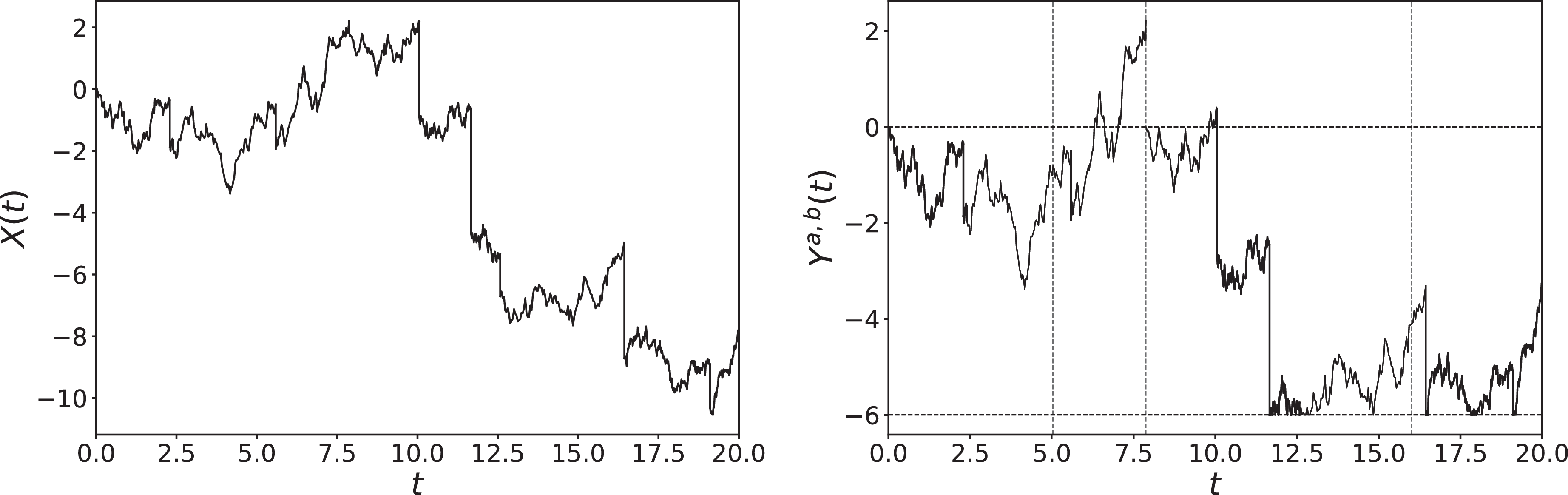


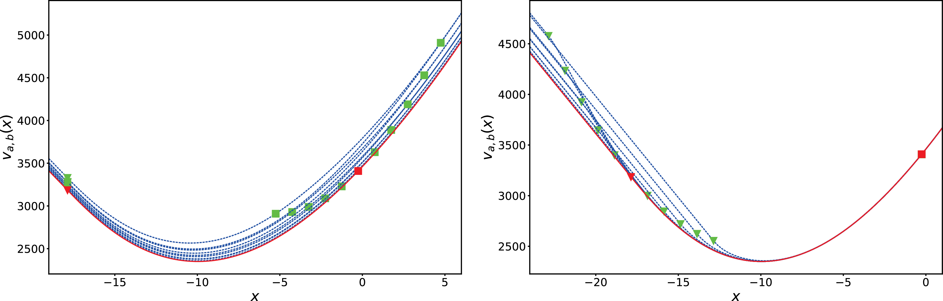


 Open access