


1. Introduction
The dominant markets where information is first discovered may play the role of price leader providing significant market information to other markets, price followers, which may have insufficient activity to generate information that is relevant to other markets (Schroeder, Reference Schroeder1996). Locating the price discovery center or market, and estimating price interactions among the regional fed and feeder cattle markets, can help define a relevant fed cattle procurement market. This study identifies dynamic price characteristics and relationships by implementing a novel technique within a time series approach that may assist market participants along the cattle supply chain, specifically in procurement strategies, price risk mitigations, and potential investment decision-making for a number of businesses. Note that there have been a series of studies with time series approaches playing a larger role in price discovery, to identify a reference cattle market, as discussed below. One challenge is that time series approaches limit the number of markets to compare even though there may be many interrelated prices, in this case at least 30-price series. Prior studies have considered at most five to six markets. This paper attempts to overcome this challenge by combining time series models with a tournament method and using both in conjunction with the cluster analysis.
The term price discovery refers to a process whereby the relative contributions of interrelated submarkets to the overall market price can be determined. The submarket with the larger contribution is called the “price discovery (market).” Several studies have investigated price leadership and delineation of the relevant geographic market for fed cattle. Koontz, Garcia, and Hudson (Reference Koontz, Garcia and Hudson1990), using weekly prices from 1973 through 1984 and Granger causality analysis, found that the Nebraska direct market responded fastest to new information. Through the vector autoregression (VAR) of weekly regional fed cattle prices from 1976 through 1987, Schroeder and Goodwin (Reference Schroeder and Goodwin1991) found that Iowa/Southern Minnesota and Eastern Nebraska tended to be the leading price discovery regions, with western Kansas becoming more dominant over the time period.
Schroeder (Reference Schroeder1996) used plant-level transaction prices (from March 23, 1992 to April 3, 1993) and applied VAR models and Granger causality analysis, finding that slaughter plants in Kansas and Nebraska tended to be price discovery leaders. Plants in other states reacted most quickly to price changes at the Nebraska plants. One recent study, Coffey, Pendell, and Tonsor (Reference Coffey, Pendell and Tonsor2019), applied error correction model (ECM), directed acyclic graph, and Granger causality analysis to weekly negotiated live steer and heifer price data from June 2001 to July 2017, seeking to identify price discovery among negotiated cattle cash prices in the five major live cattle marketing regions. Interestingly, they found that Colorado has become the price leader, which is seemingly a smaller market. As results are mixed with respect to previous studies, more research may be warranted.
Regarding studies with cattle futures prices, Oellermann, Brorsen, and Farris (Reference Oellermann, Brorsen and Farris1989) found that futures prices of feeder cattle explained cash prices but not the reverse. While the cash cattle price has a strong predictive influence on the boxed beef price, the boxed beef price plays only a marginal role in price discovery. Although causality testing can be informative, these tests focus on the impact of lagged prices on current prices (Arnade and Hoffman, Reference Arnade and Hoffman2015). Instead, in this study, relative adjustment rates, derived from the estimated (bivariate) ECM, are used to estimate price discovery weights. The technique, explained in detail in the next section, is a function of the relative ratio of the speed of adjustments in an ECM. This method has been used by Schwarz and Szakmary (Reference Schwarz and Szakmary1994), Foster (Reference Foster1996), Eun and Sabherwal (Reference Eun and Sabherwal2003), Figuerola-Ferretti and Gonzalo (Reference Figuerola-Ferretti and Gonzalo2010), and Arnade and Hoffman (Reference Arnade and Hoffman2015) to identify price discovery among related markets.
However, this technique using the ECM with the relative ratio of the speed of adjustments is applicable only for the bivariate case, that is, one cointegration vector, and not applicable for the multivariable case that may have multiple cointegrating vectors. This study suggests a novel way to overcome this problem, by using the cluster analysis and tournament approach. This newly developed technique allows us to compare many cattle market prices across regions, cattle type, and cash/futures markets. The main objective of this study is to investigate the dynamic relationships between U.S. cattle markets, across regions, cattle types, and cash/futures markets. This study attempts to determine the reference U.S. cattle price using the tournament approach and cluster analysis. This study is structured as follows. After providing a general introduction to the price discovery process, we explore the concept of price discovery and introduce cluster analysis. We then present data and the empirical results. We finally draw conclusions of the study and outline future studies.
2. Price Discovery and Cluster Analysis
2.1. Price discovery
Price discovery is about determining which market is more informative. Ward and Schroeder (Reference Ward and Schroeder2002) define price discovery as “…is the process of buyers and sellers arriving at a transaction price for a given quality and quantity of a product at a given time and place” (p. 1) when an asset or similar commodities are traded in different markets such as cattle. A number of different methods have been used to study price discovery. One of the methods is to use bivariate time series analysis with an error correction term and compare speed of adjustment between the two series (Gonzalo and Granger, Reference Gonzalo and Granger1995). The underlying idea behind price discovery can be most easily explained through a graphical example.
Let ${p_1}$
represent the cattle price in region 1 (or market 1) and let
${p_1}$
represent the cattle price in region 1 (or market 1) and let ${p_2}$
represent the price of a similar type of cattle in region 2 (or market 2). Suppose that
${p_2}$
represent the price of a similar type of cattle in region 2 (or market 2). Suppose that ${p_1}$
is higher than
${p_1}$
is higher than ${p_2}$
as shown in Figure 1 and they move together, that is, cointegrated. Suppose that, for some reasons, a shock occurs in market 1, causing
${p_2}$
as shown in Figure 1 and they move together, that is, cointegrated. Suppose that, for some reasons, a shock occurs in market 1, causing ${p_1}$
to rapidly increase (first panel, Figure 1).Footnote 1 A number of things can occur after this change. Let us assume that market 1 is the price leader. Although we will likely see a slight downward correction in
${p_1}$
to rapidly increase (first panel, Figure 1).Footnote 1 A number of things can occur after this change. Let us assume that market 1 is the price leader. Although we will likely see a slight downward correction in ${p_1}$
in market 1, we will see a much larger upward change in
${p_1}$
in market 1, we will see a much larger upward change in ${p_2}$
. These changes are demonstrated in the second panel in Figure 1. This occurs because buyers and sellers in market 2 look to market 1 to ascertain the correct price in market 2. In other words, market 1 is more informative; market 2 (follower) adjusts its price more to close the gap when the price gap widens between markets 1 and 2. Let us now assume market 2 is the price leader. In this case, traders in market 2 are much less concerned with market 1. Although there may be a slight increase in
${p_2}$
. These changes are demonstrated in the second panel in Figure 1. This occurs because buyers and sellers in market 2 look to market 1 to ascertain the correct price in market 2. In other words, market 1 is more informative; market 2 (follower) adjusts its price more to close the gap when the price gap widens between markets 1 and 2. Let us now assume market 2 is the price leader. In this case, traders in market 2 are much less concerned with market 1. Although there may be a slight increase in ${p_2}$
, market 2 is not heavily influenced by the price change in market 1. Traders in market 1, however, are still very concerned with
${p_2}$
, market 2 is not heavily influenced by the price change in market 1. Traders in market 1, however, are still very concerned with ${p_2}$
. Although the shock in market 1 causes a temporary increase in
${p_2}$
. Although the shock in market 1 causes a temporary increase in ${p_1}$
, the price in market 2 indicates to traders in market 1 that
${p_1}$
, the price in market 2 indicates to traders in market 1 that ${p_1}$
is too high. This information is incorporated into market negotiations, and, over time,
${p_1}$
is too high. This information is incorporated into market negotiations, and, over time, ${p_1}$
returns to its proper level, slightly higher than
${p_1}$
returns to its proper level, slightly higher than ${p_2}$
. This change is shown in the third panel in Figure 1.
${p_2}$
. This change is shown in the third panel in Figure 1.
Price discovery illustration.

2.2. Vector error correction model and its limitation
Since price discovery is about an identical/similar asset or commodity traded in different markets, a cointegration framework is adopted. The conventional price discovery measure used in the literature has simply compared the speed of adjustment coefficients in the bivariate vector error correction model (VECM) as a share of the total adjustment, as developed in Gonzalo and Granger (Reference Gonzalo and Granger1995) and expanded in Theissen (Reference Theissen2002). Other measures of price discovery used in the literature from a multiple market perspective are information share (IS) of Hasbrouck (Reference Hasbrouck1995) and component share (CS) of Booth et al. (Reference Booth, So and Tse1999) and Chu et al. (Reference Chu, Hsieh and Tse1999). These are discussed at length in the Journal of Financial Market’s special issue on price discovery measurement in 2002 (Baillie et al., Reference Baillie, Booth, Tse and Zabotina2002; De Jong, Reference De Jong2002; Harris et al., Reference Harris, McInish and Wood2002; Hasbrouck, Reference Hasbrouck2002; Lehmann, Reference Lehmann2002). The IS measures each market’s relative contribution to the variance of the efficient price, while the CS decomposes the common efficient price into a weighted average of observed market prices and measures each market’s contribution to the common efficient price. Both IS and CS are based on the reduced-form forecasting errors of a VECM. Yan and Zivot (Reference Yan and Zivot2010) proposed the joint use of the IS and the CS, and De Jong and Schotman (Reference De Jong and Schotman2010) developed the unobserved component approach.
The long-run equilibrium between two prices can be written as:
 $${p_{1,t}} = {\beta _2}{p_{2,t}} + c + {u_t}{\rm{\;\;}} \Leftrightarrow {\rm{\;\;}}{u_t} = {p_{1,t}} - {\beta _2}{p_{2,t}} - c$$
where ${p_{1,t}}$
and
${p_{1,t}}$
and ${p_{2,t}}$
represent prices in markets 1 and 2 at time
${p_{2,t}}$
represent prices in markets 1 and 2 at time $t$
, respectively. The term
$t$
, respectively. The term $c$
(constant term) accounts for average differences in these two markets. The term
$c$
(constant term) accounts for average differences in these two markets. The term ${u_t}$
is the (long-run) error, which is zero in equilibrium.
${u_t}$
is the (long-run) error, which is zero in equilibrium.
The bivariate VECM contains this long-run equilibrium in equation (1) as:
 $$\eqalign{ \Delta {p_{1,t}} = {\alpha _1}\left( {{p_{1,t - 1}} - {\beta _2}{p_{2,t - 1}} - c} \right) + \mathop \sum \limits_{k = 1}^{K - 1} {\gamma _{11,k}}\Delta {p_{1,t - k}} + \mathop \sum \limits_{k = 1}^{K - 1} {\gamma _{12,k}}\Delta {p_{2,t - k}} + {e_{1,t}} \cr \Delta {p_{2,t}} = {\alpha _2}\left( {{p_{1,t - 1}} - {\beta _2}{p_{2,t - 1}} - c} \right) + \sum\limits_{k = 1}^{K - 1} {{\gamma _{21,k}}} \Delta {p_{1,t - k}} + \sum\limits_{k = 1}^{K - 1} {{\gamma _{22,k}}} \Delta {p_{2,t - k}} + {e_{2,t}} \cr} $$
where $\Delta{p_{i,t}}$
represents the differenced prices. Coefficients
$\Delta{p_{i,t}}$
represents the differenced prices. Coefficients ${\alpha _1}$
and
${\alpha _1}$
and ${\alpha _2}$
are the adjustment rate parameters, and they represent the speed with which a displaced
${\alpha _2}$
are the adjustment rate parameters, and they represent the speed with which a displaced ${p_1}$
(or
${p_1}$
(or ${p_2}$
) returns to its long-run equilibrium. Using vectors and matrices, equation (2) is simplified as:
${p_2}$
) returns to its long-run equilibrium. Using vectors and matrices, equation (2) is simplified as:
 $$\Delta {{\bf{p}}_t} = {\bf{\alpha }}\left( {{\bf{\beta^\prime}}{{\bf{p}}_{t - 1}} - {\bf{c}}} \right) + \mathop \sum \limits_{k = 1}^{K - 1} {{\bf{\Gamma }}_k}\Delta {{\bf{p}}_{t - k}} + {{\bf{e}}_t} = {\bf{\Pi }}\left( {{{\bf{p}}_{t - 1}} + {\bf{\mu }}} \right) + \mathop \sum \limits_{k = 1}^{K - 1} {{\bf{\Gamma }}_k}\Delta {{\bf{p}}_{t - k}} + {{\bf{e}}_t}$$
where ${\bf{\alpha '}} = \left[ {{\alpha _1},{\alpha _2}} \right]$
is 2×1 vector of adjustment coefficients (speed of adjustment),
${\bf{\alpha '}} = \left[ {{\alpha _1},{\alpha _2}} \right]$
is 2×1 vector of adjustment coefficients (speed of adjustment), ${\bf{\beta '}} = \left[ {1,{\beta _2}} \right]$
is 2×1 cointegrating vector,
${\bf{\beta '}} = \left[ {1,{\beta _2}} \right]$
is 2×1 cointegrating vector, ${\bf{c}}$
is an intercept,
${\bf{c}}$
is an intercept, ${\bf{\Pi }} = {\bf{\alpha \beta '}}$
, and
${\bf{\Pi }} = {\bf{\alpha \beta '}}$
, and ${\bf{\mu }} = - {{\bf{\Pi }}^{ - 1}}{\bf{c}}$
.
${\bf{\mu }} = - {{\bf{\Pi }}^{ - 1}}{\bf{c}}$
. $\;\;K$
is the lag-length of the VAR and
$\;\;K$
is the lag-length of the VAR and ${{\bf{e}}_t}$
is the reduced-form shock.
${{\bf{e}}_t}$
is the reduced-form shock.
Following Gonzalo and Granger (Reference Gonzalo and Granger1995), the relative ratio of the adjustment coefficients is defined by
 $${\theta _1} = {{\left| {{\alpha _2}} \right|} \over {\left| {{\alpha _1}} \right| + \left| {{\alpha _2}} \right|}},{\rm{}}{\theta _2} = {{\left| {{\alpha _1}} \right|} \over {\left| {{\alpha _1}} \right| + \left| {{\alpha _2}} \right|}},\;{\rm{and}}\;{\theta _1} + {\theta _2} = 1$$
A high $\theta \;$
indicates a low
$\theta \;$
indicates a low $\alpha $
(speed of adjustment toward a new long-run equilibrium), which implies that this market slowly responds to an unpredicted shock in the system; therefore, the market is the price discovery reference market. If
$\alpha $
(speed of adjustment toward a new long-run equilibrium), which implies that this market slowly responds to an unpredicted shock in the system; therefore, the market is the price discovery reference market. If ${\theta _1} = {\theta _2}=0.5$
, both markets contribute equally to the price discovery process, that is, both markets move at a similar rate toward the long-run equilibrium. Note that
${\theta _1} = {\theta _2}=0.5$
, both markets contribute equally to the price discovery process, that is, both markets move at a similar rate toward the long-run equilibrium. Note that ${\theta _i}$
is applicable only for the bivariate case with
${\theta _i}$
is applicable only for the bivariate case with ${{\bf{\alpha }}_{2 \times 1}}$
. For the multivariate case with one cointegrating vector, we may arrange price discovery according to relative magnitude of
${{\bf{\alpha }}_{2 \times 1}}$
. For the multivariate case with one cointegrating vector, we may arrange price discovery according to relative magnitude of ${\alpha _i}$
, but it is not clear how to calculate
${\alpha _i}$
, but it is not clear how to calculate ${\theta _i}$
. Moreover, if there are multiple cointegrating vectors, comparing price discovery using
${\theta _i}$
. Moreover, if there are multiple cointegrating vectors, comparing price discovery using ${\alpha _i}$
is not applicable.
${\alpha _i}$
is not applicable.
However, an Achilles heel to price discovery using the speed of adjustment coefficients with the VECM outlined in equations (2) and (4) is its inability to compare more than two variables at a time. This is because there must be one cointegrating relationship between the relevant variables. For the multivariate case with one cointegrating relation, we may arrange price discovery according to relative magnitude of ${\alpha _i}$
but it is not clear how to calculate
${\alpha _i}$
but it is not clear how to calculate ${\theta _i}$
. Another shortcoming is that some markets may result in possibly having a negative weight generated from potential collinearity. In addition, in the multivariate case there might be more than one cointegrating relationship. For n time series, there might be as many as n−1 cointegrating relationships. Since there is no way of choosing in this latter case which of these possible cointegrating relationships to use in the model (Kim, Reference Kim2011), one cannot use this approach to compare more than two series at a time. This is a limitation when examining markets of a commodity, which almost always involves more than two markets, such as cattle markets.
${\theta _i}$
. Another shortcoming is that some markets may result in possibly having a negative weight generated from potential collinearity. In addition, in the multivariate case there might be more than one cointegrating relationship. For n time series, there might be as many as n−1 cointegrating relationships. Since there is no way of choosing in this latter case which of these possible cointegrating relationships to use in the model (Kim, Reference Kim2011), one cannot use this approach to compare more than two series at a time. This is a limitation when examining markets of a commodity, which almost always involves more than two markets, such as cattle markets.
2.3. Cluster analysis and tournament
As noted, when there are multiple markets, this technique, equation (4), may not be applicable. The tournament approach using cluster analysis provides a way to overcome this problem as demonstrated in Kim, Tejeda, and Wright (Reference Kim, Tejeda and Wright2016). Cluster analysis divides cattle price data into groups (clusters) that are meaningful, useful, or both (Tan, Steinbach, and Kumar, Reference Tan, Steinbach and Kumar2006). It implements a hierarchy using various techniques, for example, pairwise distance between all data points. Once the cluster analysis provides the resulting cluster(s), the sequential VECM approach (similar to a tournament) is applied and we can identify the price discovery region(s) for each hierarchy. The main contribution of this paper is the development of a technique that allows the researcher to compare many markets at once.
Early attempts at overcoming this problem included a round robin tournament approach. This means using the ECM to compare each series to every other series. This method may be inefficient and labor intensive, as growth in the number of markets being studied involves a substantial increase in the number of comparisons. An approximation to a round robin tournament approach was a study by Oellermann, Brorsen, and Farris (Reference Oellermann, Brorsen and Farris1989) which considered four markets: labeled feeder futures, feeder cash, live cattle cash, and live cattle futures. The authors compared four pairs of variables: (1) feeder cash vs. feeder futures, (2) feeder cash vs. live cattle futures, (3) feeder cash vs. live cattle cash, and (4) feeder futures vs. live cattle futures. Nonetheless, it was technically not a round robin tournament since possible combinations such as (5) live feeder futures vs. live cattle futures and (6) live cattle futures vs. live cattle cash were not included.
Another, more efficient, approach is to use a single elimination tournament. Our paper uses a single elimination tournament. Using this approach in a study with $n$
markets allows us to reduce the number of comparisons to
$n$
markets allows us to reduce the number of comparisons to $n - 1$
. For example, if one were to do a study including prices from 30 different markets, one would only have to run the 29 bivariate VECMs. A downside to a single elimination tournament is we cannot say who the second strongest competitor is. Just because a competitor loses in the final round does not mean it is second strongest. The second, third, and fourth strongest competitors may have already been matched against the strongest competitor and eliminated by the time the final round is played.
$n - 1$
. For example, if one were to do a study including prices from 30 different markets, one would only have to run the 29 bivariate VECMs. A downside to a single elimination tournament is we cannot say who the second strongest competitor is. Just because a competitor loses in the final round does not mean it is second strongest. The second, third, and fourth strongest competitors may have already been matched against the strongest competitor and eliminated by the time the final round is played.
Sports tournaments often address this issue through the use of double and triple elimination tournaments. In a double elimination tournament, one must lose twice before being eliminated. The tournament is designed so that if two teams play each other once, they do not play each other again until the final round. This ensures the second strongest team makes it to the final round before being eliminated. The triple elimination tournament works on the same principle except it ensures the top three teams make it to the final stages of the tournament. Unfortunately, a double elimination tournament requires twice as many matches as a single elimination tournament. A triple elimination tournament requires three times as many matches, etc. Rather than use a double or triple elimination tournament, along with the cumbersome load it would entail, we will use a single elimination tournament by incorporating a cluster analysis. We will use this data mining tool to segregate our variables into groups or clusters, allowing us to identify “winners” in subcategories of the U.S. cattle market.
To perform a cluster analysis means nothing more than dividing data into groups. This is usually done to make the data more meaningful, useful, or both (Tan, Steinback, and Kumar, Reference Tan, Steinbach and Kumar2006, p. 487). During this process of grouping, a set of data or other objects are sorted into multiple groups so that objects within a cluster have high similarity, but are less similar to objects in other clusters. Sameness can be based on whatever factors the researcher considers relevant. Quite often, differences involve distance measures. Regardless of difference criteria, the goal of this process is to create clusters where the objects within a group are similar to one another and different from the objects in the other groups. Greater similarity within a group and larger differences between groups are usually preferred, since this leads to more distinct clustering.
With time series data, like that used in this study, the most popular distance measure is Euclidean distance. Let ${p_{i,t}}$
be the (cattle) price in market
${p_{i,t}}$
be the (cattle) price in market $i\,=\,1, \cdots ,n$
. The Euclidean distance between markets
$i\,=\,1, \cdots ,n$
. The Euclidean distance between markets $i$
and
$i$
and $j$
is defined as follows:
$j$
is defined as follows:
 $$d\left( {i,j} \right) = \sqrt {\mathop \sum \limits_{t = 1}^T {{\left( {{p_{i,t}} - {p_{j,t}}} \right)}^2}} $$
Note that the Euclidean distance is nonnegative, the distance of a market to itself is 0, that is, $d\left( {i,i} \right) = 0$
and the distance is symmetric, that is,
$d\left( {i,i} \right) = 0$
and the distance is symmetric, that is, $d( {i,j}) = d({j,i})$
. Equation (5) is converted to the root mean square deviation (RMSD) if the expression inside the square root is divided by
$d( {i,j}) = d({j,i})$
. Equation (5) is converted to the root mean square deviation (RMSD) if the expression inside the square root is divided by $T$
. A limitation of using equation (5) for the cattle market is of not accounting for different economic factors on how the market prices are determined. Prices may vary based on transportation costs, seasonality, product transformation, etc. (i.e. heterogeneous). These factors may create large differences between the prices of markets being considered as centers of price discovery. Thus, the differences in prices may reflect many potential economic factors that may not be price discovery related. Future work considers methods that account for these economic factors within the price equilibrium relationships.
$T$
. A limitation of using equation (5) for the cattle market is of not accounting for different economic factors on how the market prices are determined. Prices may vary based on transportation costs, seasonality, product transformation, etc. (i.e. heterogeneous). These factors may create large differences between the prices of markets being considered as centers of price discovery. Thus, the differences in prices may reflect many potential economic factors that may not be price discovery related. Future work considers methods that account for these economic factors within the price equilibrium relationships.
Clustering comes in different types, including nested and unnested, that is, partitional or hierarchical. In a partitional clustering, the set of data objects is sorted into non-overlapping subsets (clusters) so that each object is in one, and only one, subset. To obtain a hierarchical clustering, we permit clusters to have subclusters, which are a set of nested clusters. Graphical representations of clusters resemble a tree.
A hierarchical clustering method works by grouping markets into a tree of subclusters. We can further divide hierarchical clustering methods into two types: (i) agglomerative hierarchical clustering and (ii) divisive hierarchical clustering. The first type, agglomerative hierarchical clustering, is based on a bottom-up strategy. It usually starts by letting one object form a cluster and forms successively larger clusters around the original one, until all objects have been sorted. The single cluster is the starting point for the hierarchy. A divisive hierarchical clustering method works in the opposite direction. It starts by placing all the objects in one group. The group is then split into several smaller groups. These smaller groups are then each partitioned into even smaller groups. This process is repeated until objects within each group are similar enough to each other. Figure 2 shows an agglomerative hierarchical clustering method and a divisive hierarchical clustering method, on a data set of five objects, $\left\{ {a,\;b,\;c,\;d,\;e} \right\}$
. Initially, the agglomerative method places each object into a cluster of its own. The clusters are then merged step-by-step according to some criterion. For example, clusters
$\left\{ {a,\;b,\;c,\;d,\;e} \right\}$
. Initially, the agglomerative method places each object into a cluster of its own. The clusters are then merged step-by-step according to some criterion. For example, clusters ${C_1}$
and
${C_1}$
and ${C_2}$
may be merged if an object in
${C_2}$
may be merged if an object in ${C_1}$
and an object in
${C_1}$
and an object in ${C_2}$
form the minimum Euclidean distance between any two objects from different clusters. This is a single-linkage approach in that each cluster is represented by all the objects in the cluster, and the similarity between two clusters is measured by the similarity of the closest pair of data points belonging to different clusters.
${C_2}$
form the minimum Euclidean distance between any two objects from different clusters. This is a single-linkage approach in that each cluster is represented by all the objects in the cluster, and the similarity between two clusters is measured by the similarity of the closest pair of data points belonging to different clusters.
Dendrogram representation for hierarchical clustering. (Reproduced from fig. 10.6 in Han, Kamber, and Pei (Reference Han, Kamber and Pei2012), p. 460).

The cluster-merging process repeats until all the objects are eventually merged to form one cluster. The divisive method proceeds in the contrasting way. All the objects are used to form one initial cluster. The cluster is split according to some principle such as the maximum Euclidean distance between the closest neighboring objects in the cluster. The cluster-splitting process repeats until, eventually, each new cluster contains only a single object. A tree structure, called a dendrogram, is commonly used to represent the process of hierarchical clustering. It shows how objects are grouped together (in an agglomerative method) or partitioned (in a divisive method) step-by-step. Figure 2 shows a dendrogram for the five objects presented in Figure 2, where $l\,=\,0$
shows the five objects as singleton clusters at level 0. At
$l\,=\,0$
shows the five objects as singleton clusters at level 0. At $l\,=\,1$
, objects
$l\,=\,1$
, objects $a$
and
$a$
and $b$
are grouped together to form the first cluster, and they stay together at all subsequent levels. We can also use a vertical axis to show the similarity scale between clusters. For example, when the similarity of two groups of objects
$b$
are grouped together to form the first cluster, and they stay together at all subsequent levels. We can also use a vertical axis to show the similarity scale between clusters. For example, when the similarity of two groups of objects $\left\{ {a,\;b} \right\}$
and
$\left\{ {a,\;b} \right\}$
and $\left\{ {c,\;d,\;e} \right\}$
is roughly 0.16 (similarity scale on the right in Figure 3), they are merged together to form a single cluster.
$\left\{ {c,\;d,\;e} \right\}$
is roughly 0.16 (similarity scale on the right in Figure 3), they are merged together to form a single cluster.
Cluster analysis dendrogram.
Notes: (1) State_fed_S = fed cattle steer in state; State_fed_H = fed cattle heifer in state; State Name_feeder_S = feeder cattle steer in state; State Name_feeder_H = feeder cattle heifer in state. (2) Vertical axis, Height, is the Euclidean distance between markets; height of 100 is approximately $3.5/cwt difference between markets (see equation (5)). (3) Boxes cut and visualize the dendrogram to five clusters (authors’ choice).

In this research, the hclust function in R software is utilized. This program uses the maximum distance, ${d_{max}}\left( {{C_i},{C_j}} \right) = \mathop {\max }_{{p \in {C_i},p' \in {C_j}}} \left\{ \left| {p - p'} \right|\right\} $
, where
${d_{max}}\left( {{C_i},{C_j}} \right) = \mathop {\max }_{{p \in {C_i},p' \in {C_j}}} \left\{ \left| {p - p'} \right|\right\} $
, where $\left| {p - p'} \right|$
is the distance between two markets, to measure the distance between clusters. It is sometimes called a complete-linkage algorithm.
$\left| {p - p'} \right|$
is the distance between two markets, to measure the distance between clusters. It is sometimes called a complete-linkage algorithm.
3. Data and Tests
3.1. Cattle price data
This study uses weekly cattle price data from May 2001 through October 2016. All cattle cash and futures price data are obtained from the Livestock Marketing Information Center (LMIC), which compiled the U.S. Department of Agriculture Agricultural Marketing Service (USDA-AMS) Livestock Mandatory Price Reporting (LMR) report data. The fed cattle price data were collected from all Free on Board (FOB) negotiated trade prices within a region. Regions studied include Texas–New Mexico–Oklahoma (TX–NM–OK), Kansas (KS), Nebraska (NE), Colorado (CO), and Iowa–Minnesota (IA-MN). A weekly fed cattle price for each region represents the weighted average from the steers and heifers prices. All weights and grades of cattle were included in this calculation. For feeder cattle price, only calves from 500 to 900 pounds were included. Data from all the auctions in the relevant geographical area were included. Regions studied include CO, KS, Missouri (MO), Montana (MT), NE, OK, South Dakota (SD), and TX. The raw data gave an average price for steers and heifers, divided into categories by hundred-pound increments. Head counts from these auctions were not available at the time of this study. A simple, unweighted average was calculated for both steers and heifers considering the specified weight ranges.Footnote 2
Unfortunately, both the fed cattle price and the feeder cattle price series contained missing observations. The data set was made complete by taking an average of the observations above and below the missing point and using this estimate of the missing observation. If there was more than one missing observation in a row, the missing points were estimated to be contained in a line between the closest observable points (linear interpolation). In addition, an extensive number of typos were present in the raw feeder cattle price data. Prices greater than $3/cwt were removed from the data, and these missing observations were estimated using linear interpolation. The price level of $3/cwt was chosen to maximize the amount of data retained, while still eliminating outliers and probable mistakes in the raw data.
Boxed beef cutout price is also included and it is provided by the weekly average beef cutout prices for Choice 600–900 lbs. from the “National Weekly Boxed Beef Cutout and Boxed Beef Cuts—Negotiated Sales” report by the Agricultural Marketing Service of the USDA and obtained from LMIC. The raw boxed beef cutout data had no missing observations and were used as provided. In addition to these prices, the feeder cattle index is included. The feeder cattle index is a 7-day weighted average of the total dollars sold divided by the total pounds during the same period. The feeder cattle index is included to gauge the level of the potential price discovery type of information that the index could possibly provide. The USDA-AMS issues daily reports which contain cattle eligible for the index. Cattle futures prices are collected from LMIC as well, which was compiled from Chicago Mercantile Exchange. The futures prices are of nearby contracts referring to the contracts’ close price that is closest to expiration. It rolls over on the first date of the new month after the preceding contracts end. The weekly averages are calculated by taking the previous Monday–Friday for the week ending on a Friday data. In total, we have 30 cattle price series which are the combinations of regions, feeder/fed, steer/heifer, and futures prices. Table 1 presents basic statistics.
Basic statistics (dollars per cwt)

Source: Livestock Marketing Information Center (LMIC).
State Name_fed_S = fed cattle steer in state; State Name_fed_H = fed cattle heifer; State Name_feeder_S = feeder cattle steer; State Name_feeder_H = feeder cattle heifer.
3.2. Stationary tests and cointegration tests
Before moving to cointegration tests to check if there exists one cointegrating relationship among pairs of series, stationarity tests for each price series were conducted. This study utilizes the Phillips Perron test to check for stationarity of each variable (Phillips and Perron, Reference Phillips and Perron1988). As expected, all the cattle prices are non-stationary (results are not reported to save space). All matched series were tested for cointegration using the Johansen’s trace test, and all were found to be cointegrated. The fact that all these pairs are cointegrated makes them suitable for analysis with the ECM. The optimal lag of VECM is determined using the Schwarz information criterion. The number of cointegration relationship in the bivariate case is at most one cointegrating vector and can be investigated based on likelihood ratio (LR)-type tests (Lütkepohl and Krätzig, Reference Lütkepohl and Krätzig2004). Johansen (Reference Johansen1995) provides critical values for the LR test, which is known as the trace test.
4. Results
4.1. Cluster analysis
The cluster analysis provides the cluster dendrogram as shown in Figure 3. As can be seen from the dendrogram, this clustering creates a special kind of tournament bracket. In this bracket, those markets most closely aligned with each other are compared first. The advantage of this approach is that it allows us to draw more conclusions about segments of the market than would be possible if we randomly assigned variables to different places in a single elimination tournament. For instance, all the fed cattle markets are grouped into the same hierarchy (second blue box in Figure 3). This allows us to determine the price discovery for the U.S. fed cattle market. The implications of this approach will be made clearer subsequently.
The cluster analysis allows us to draw conclusions about market structure from the height of the clusters that is shown to the left of the dendrogram in Figure 4. As previously explained in equation (5), this number represents the Euclidian distance between markets $i$
and
$i$
and $j$
. We can use this equation (5) to calculate the RMSDs, which is
$j$
. We can use this equation (5) to calculate the RMSDs, which is
 $${\rm{RMSD}} \approx \sqrt {{{{{d\left( {i,j} \right)}^2}} \over T}} $$
where $T$
is the total number of observations.
$T$
is the total number of observations.
Fed cattle tournament result.
Notes: (1) State_fed_S = fed cattle steer in state; State_fed_H = fed cattle heifer in state. (2) Vertical axis, Height, is the Euclidean distance between markets; height of 100 is approximately $3.5/cwt difference between markets (see equation (7)). Blue boxes cut and visualize the dendrogram to four clusters (authors’ choice). (3) Numbers are relative adjustment coefficients, that is, ${\theta _i}$
in equation (4); between two comparing markets, the winner has a larger
${\theta _i}$
in equation (4); between two comparing markets, the winner has a larger $\theta $
.
$\theta $
.

We can now use the appropriate numbers to see how much price variation occurs in the different cattle markets. For instance, we can see from the dendrogram in Figure 4 that the height on the box containing the fed cattle markets (second box in Figure 4) is approximately 100. We have 809 observations. So, the RMSD in price for the time periods examined for the two series furthest apart in the fed market is $3.52.Footnote 3 In contrast, the height for the feeder market is about 700. This gives the RMSD, within the feeder market of $24.60.
Although the original intent of this paper was to determine the price discovery for the entire U.S. cattle market, the cluster analysis demonstrates the submarkets within this industry are separate enough from each other that they should be viewed as separate markets, rather than subcategories within the same market. The distance, for example, between the fed and feeder markets is approximately 1,200. This translates to the RMSD at each time period of $42.16. The distance between the boxed beef market and the other markets studied is about 2,000. This translates into an average price spread of $70.27. Although there are obvious connections between these markets, these large price spreads demonstrate the significant separations between these markets. This is at least partially due to boxed beef prices being in different units, as they are in price per wholesale pound rather than live pound. Due to these conditions, we identify the price discovery for the fed market as well as the feeder market. We do not, however, attempt to determine a winner between the two. From this point forward, we also view boxed beef as a separate market, excluding it from our analysis.
The submarkets identified by the cluster analysis include the following:
-
1. Fed cattle market: this market includes all fed cattle price series as well as fed cattle futures (second blue box in Figure 3).
-
2. Feeder cattle market
-
a. Feeder steer market: this market includes all feeder steers except those from Texas (third blue box in Figure 3).
-
b. Feeder heifer and feeder futures market: this market includes all feeder heifers, feeder cattle futures, the feeder cattle index, and feeder steers from Texas (fourth and fifth blue box in Figure 3).
-
We examine these submarkets and then compare the winners from each category. A VECM for each pair of these submarkets is estimated, we then determine the price discovery region using values of ${\theta _i}$
from equation (4), and the leader of each binary contest goes up one hierarchy. Another VECM is estimated for the new (hierarchical) pair of markets and then the price discovery region is identified until we have the final “winner.”
${\theta _i}$
from equation (4), and the leader of each binary contest goes up one hierarchy. Another VECM is estimated for the new (hierarchical) pair of markets and then the price discovery region is identified until we have the final “winner.”
4.2. The tournament results of the fed cattle market
The first group we examine is the fed cattle market. Figure 4 summarizes the results. Figure 5 includes the name of the series being compared, followed by ${\theta _i}$
in equation (4) using the adjustment coefficients from the corresponding VECM. The results of relative adjustment coefficients are given in Table A1 in the appendix. For instance, the bottom left corner of the diagram shows the comparison between CO fed steer and CO fed heifer. The
${\theta _i}$
in equation (4) using the adjustment coefficients from the corresponding VECM. The results of relative adjustment coefficients are given in Table A1 in the appendix. For instance, the bottom left corner of the diagram shows the comparison between CO fed steer and CO fed heifer. The $\theta $
value for the CO fed steer is 0.299, and the
$\theta $
value for the CO fed steer is 0.299, and the $\theta $
value for CO fed heifer is 0.701. Clearly, this indicates CO fed heifer is the winner for this round in the tournament. Consequently, it moves forward to compete against NE fed steer which is a winner of NE fed steer and NE fed heifer match. It is noteworthy that the dendrogram and winners of the fed cattle market in Figure 5 are similar to the size of the negotiated live cattle sales in recent years. In 2014–2018, NE had the largest share of 0–30-day negotiated cattle sales represented at 37% followed by IA at 21% and KS 17% (Schroeder, Schulz, and Tonsor, Reference Schroeder, Schulz and Tonsor2019). Earlier studies by Bailey and Brorsen (Reference Bailey and Brorsen1985) found that TX was the center of price discovery; however, Schroeder and Goodwin (Reference Schroeder and Goodwin1990) identified Iowa–Nebraska as the leading price discovery locations; thus, changes in negotiated sales may have played a role.
$\theta $
value for CO fed heifer is 0.701. Clearly, this indicates CO fed heifer is the winner for this round in the tournament. Consequently, it moves forward to compete against NE fed steer which is a winner of NE fed steer and NE fed heifer match. It is noteworthy that the dendrogram and winners of the fed cattle market in Figure 5 are similar to the size of the negotiated live cattle sales in recent years. In 2014–2018, NE had the largest share of 0–30-day negotiated cattle sales represented at 37% followed by IA at 21% and KS 17% (Schroeder, Schulz, and Tonsor, Reference Schroeder, Schulz and Tonsor2019). Earlier studies by Bailey and Brorsen (Reference Bailey and Brorsen1985) found that TX was the center of price discovery; however, Schroeder and Goodwin (Reference Schroeder and Goodwin1990) identified Iowa–Nebraska as the leading price discovery locations; thus, changes in negotiated sales may have played a role.
Feeder cattle heifer tournament result.
Notes: (1) State Name_feeder_S = feeder cattle steer in state; State Name_feeder_H = feeder cattle heifer in state. (2) Vertical axis, Height, is the Euclidean distance between markets; height of 100 is approximately $3.5/cwt difference between markets (see equation (7)). Blue boxes cut and visualize the dendrogram to four clusters (authors’ choice). (3) Numbers are relative adjustment coefficients, that is, ${\theta _i}$
in equation (4); between two comparing markets, the winner has a larger
${\theta _i}$
in equation (4); between two comparing markets, the winner has a larger $\theta $
.
$\theta $
.

Although this is a single elimination tournament, comparison of pairs of series through the structure provided by the cluster analysis allows us to conclude NE fed steer is the price discovery when only fed cattle price markets are considered, that is, as shown in Figure 5, NE fed steer plays an important part in the price discovery process. However, when we compare fed futures to NE fed steer, we see the price is actually discovered in the fed futures market. This confirms the results from an extensive literature on futures markets going back at least to the early 1940s (Working, Reference Working1942).
4.3. The tournament results of feeder heifer and feeder futures markets
The second group includes the feeder heifers, feeder futures, the feeder index, and TX feeder steers (Figure 5). This bracket exemplifies some of the weaknesses of our approach. The feeder index contains more information than any of the particular live feeder markets. Yet, because it lies closest to feeder futures, it is eliminated without being compared to any of the live feeder markets. One might be tempted to conclude from the diagram that KS feeder heifer plays a prominent role in the price discovery process. This, however, would be a mistake. A closer examination of the bracket reveals KS feeder heifer could actually be less important in the price discovery process than the feeder index, feeder futures, NE feeder heifers, SD feeder heifers, and TX feeder steers. This would place KS feeders somewhere in the middle of the pack, rather than in second place. The one conclusion we can draw is that feeder futures is the price discovery in this subdivision of the U.S. cattle market.
4.4. The tournament results of feeder cattle steers
The third group includes all the feeder steers except those from TX. As the diagram in Figure 6 shows, CO feeder steers are the price discovery out of the variables compared. It is still necessary to compare the winner from the feeder cattle heifers tournament with the winner from the feeder cattle steers tournament. When we do this, we find the $\theta $
value for Colorado feeder steers to be 0.380 and the
$\theta $
value for Colorado feeder steers to be 0.380 and the $\theta $
value for feeder futures to be 0.620. As explained in the section on fed cattle markets, this result confirms a large body of research showing the correct price for commodities is discovered in the futures market.
$\theta $
value for feeder futures to be 0.620. As explained in the section on fed cattle markets, this result confirms a large body of research showing the correct price for commodities is discovered in the futures market.
Feeder cattle steers tournament result.
Notes: (1) State Name_feeder_S = feeder cattle steer in state; State Name_feeder_H = feeder cattle heifer in state. (2) Vertical axis, Height, is the Euclidean distance between markets; height of 100 is approximately $3.5/cwt difference between markets (see equation (5)). Blue boxes cut and visualize the dendrogram to 4 clusters (authors’ choice). (3) Numbers are relative adjustment coefficients, that is, ${\theta _i}$
in equation (4); between two comparing markets, the winner has a larger θ.
${\theta _i}$
in equation (4); between two comparing markets, the winner has a larger θ.

5. Summary and Concluding Remarks
Price discovery in cattle markets is a topic of interest for professionals working in the industry as well as for economists. This study investigates the dynamic relationships of 30 cattle markets across regions, cattle types, and cash/futures markets. Determining price discovery process among a very large number of related markets is not efficiently workable. The comparison of many markets, using an ECM, is accomplished with the introduction of a tournament with a hierarchical cluster analysis, which allows us to conclude that the appropriate price for the U.S. cattle markets is discovered in the futures markets for both feeder and fed cattle.
The major contribution of this paper is the tournament approach with a cluster analysis.Footnote 4 The paper discusses different kinds of tournaments that can be used, along with their strengths and weaknesses. In the end, a cluster analysis approach was adopted. An extensive discussion on different approaches to cluster analysis was presented. The use of a cluster analysis allows to avoid the cumbersome load imposed by a round robin tournament and still tease out more information than would be possible with a random single elimination tournament.
The variables were tested and it was found they all met the criteria for the ECM. The cluster analysis was conducted, and the resulting dendrogram was used to construct a single elimination tournament. The tournament was conducted using the estimated (bivariate) ECMs to determine winners and losers. The final results of the tournament confirmed theoretic expectations as well as previous empirical work done on this topic. This study shows the proper price for cattle is discovered in the futures market. It is noteworthy to mention that market weights and overall results were obtained using the distance function from equations (5) and (6), for example, steer and heifer prices being separated in different clusters. As noted earlier, these results may change if a different metric is used to measure the difference between the markets’ equilibrium prices, for example, a method that incorporates economic factors that vary among the markets (e.g. transportations costs). The objective of this study was to provide a novel method to address a challenging dynamic price discovery process that has too many prices and to provide a way to simplify it. Limitations and future lines of study regarding cattle markets, or others, are below. The aim of this study was to provide a fair approximation of this process that has too many markets, while addressing the econometric challenge.
6. Limitations and Future Work
This study extends the literature by providing a method for the comparison of a large number of series in the price discovery process; however, there are limitations and still much work to be done. First, clustering cattle markets using the price Euclidean difference (or distance) may limit the segmentation of markets as there may be two prices which are relatively far apart in distance but potentially move together. Also, it is possible that prices differ based on transportation costs, seasonality, and product transformation (levels of supply chain) which are not price discovery related. In addition, aggregating price series using a simple average, even though it provides a good approximation, may mask the valid differences among the price series. Future study will focus on fewer cattle markets, specifically breaking up feeder calf prices. Moreover, use of feeder price index, an artificially created price series that overlaps with some of the cattle price data, will be part of this future study. Second, some of the markets could be equally important. In other words, values of $\theta $
in equation (4) are similar and not statistically significant. It is hard to decide which market is a winner for that case. To proceed the discussion we may decide a winner, ignoring the relative importance of the markets. However, the flexibility and continuous weighing of markets might be one of the advantages of the Gonzalo and Granger (Reference Gonzalo and Granger1995) approach over Granger causality test which is discrete. Third, a tournament method in conjunction with cluster analysis is used in this paper to expand the Gonzalo and Granger (Reference Gonzalo and Granger1995) approach, enabling the examination of multiple markets. In addition, this is not the only way to expand the Gonzalo and Granger (Reference Gonzalo and Granger1995) approach. It suffers from the limitations inherent in single elimination tournament design. If the second strongest competitor is paired against the (resulting) strongest early in the tournament, it will be eliminated long before the final round. Thus, relative ranking of all variables is not possible with this approach. Using the ECM to make all possible comparisons between the variables and counting the number of wins would allow one to present a complete ranking of the importance of all the variables compared in the price discovery process. This, and other further refinements, should provide avenues for further exploration of the price discovery concept. In addition, it is obvious whether the losers in tournaments are responding to their cluster leader (winner) or there is a response to market leader (last winner of the tournament) beyond their own cluster leader.
$\theta $
in equation (4) are similar and not statistically significant. It is hard to decide which market is a winner for that case. To proceed the discussion we may decide a winner, ignoring the relative importance of the markets. However, the flexibility and continuous weighing of markets might be one of the advantages of the Gonzalo and Granger (Reference Gonzalo and Granger1995) approach over Granger causality test which is discrete. Third, a tournament method in conjunction with cluster analysis is used in this paper to expand the Gonzalo and Granger (Reference Gonzalo and Granger1995) approach, enabling the examination of multiple markets. In addition, this is not the only way to expand the Gonzalo and Granger (Reference Gonzalo and Granger1995) approach. It suffers from the limitations inherent in single elimination tournament design. If the second strongest competitor is paired against the (resulting) strongest early in the tournament, it will be eliminated long before the final round. Thus, relative ranking of all variables is not possible with this approach. Using the ECM to make all possible comparisons between the variables and counting the number of wins would allow one to present a complete ranking of the importance of all the variables compared in the price discovery process. This, and other further refinements, should provide avenues for further exploration of the price discovery concept. In addition, it is obvious whether the losers in tournaments are responding to their cluster leader (winner) or there is a response to market leader (last winner of the tournament) beyond their own cluster leader.
Acknowledgments
This research was supported by the Utah Agricultural Experiment Station, Utah State University and approved as journal paper number UAES9391, and also supported by USDA NIFA, Hatch project IDA 01581, and the Idaho Agricultural Experiment Station, University of Idaho. The authors appreciate the valuable comments of four anonymous reviewers.
Appendix
Speed of adjustment and relative adjustment coefficients
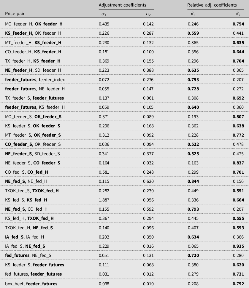
Note: A high $\theta $
means low
$\theta $
means low $\alpha $
and the market does not respond to the unpredicted shock in the market. It implies the market with a higher
$\alpha $
and the market does not respond to the unpredicted shock in the market. It implies the market with a higher $\theta $
value is the price discovery. Winners of the tournament, that is, price discovery, are indicated in bold font.
$\theta $
value is the price discovery. Winners of the tournament, that is, price discovery, are indicated in bold font.


 Open access