Review of literature

Methodology

The goal of technical efficiency analysis is to determine whether, for any specific firm observation, it is possible to simultaneously expand good outputs and/or contract inputs and bad outputs. That expansion and contraction are done in reference to the set of all firms which define the production set and thus the frontier or boundary of the production set. There are a number of methods to operationalize expansion and contraction.

We use Färe and Grosskopf’s (Reference Färe and Grosskopf2010) DDF-SBM specification to measure efficiency, which is a non-parametric DEA-type model. Compared to parametric regression-based models, the advantage of DEA-based models is that they essentially allow estimation of unique efficiency by specified inputs, outputs, and NPLs. We also avoid the defects of parametric measures, such as the requirement of assuming functional forms for both the frontier and the distribution of efficiency (Neff et al. Reference Neff, Dixon and Zhu1994). However, there are two major issues with using DEA-based models. The first is that DEA models do not directly include measurement errors in estimation. The second is that the data may represent a sample from the population. The method introduced by Simar and Wilson (Reference Simar and Wilson1998) allows bootstrapping DEA estimates to address these issues and generate confidence intervals around the point estimates. However, we use the entire population of Associations in the FCS during each data period and thus have the entire population of Associations. In addition, the data used are from FCA Call Reports, which are collected for oversight and monitoring. It is reasonable to assume that careful effort is expended in reporting these data, with oversight and auditing by the FCA, with few measurement errors.

Endogeneity in production economics, where inputs determined by the decision maker may be correlated with the error term, was first stated by Marschak and Andrews (Reference Marschak and Andrews1944) and acknowledged in estimating firm-level production functions by Mundlak (Reference Mundlak1961). Olley and Pakes (Reference Olley and Pakes1996) and Levinsohn and Petrin (Reference Levinsohn and Petrin2003) have developed approaches to alleviate endogeneity, and endogeneity has recently been a discussion point in estimating SFA and DEA efficiency (Corderoa et al. Reference Corderoa, Santínb and Siciliab2015). Endogeneity is an issue that we do not attempt to address.

We measure input and output efficiencies of each Association for each quarter under the current technology present each quarter and we do not measure technological change over time. Technological change undoubtedly occurred in the FCS as in other financial institutions, but efficiency measurement is our only interest. However, one reason an Association may become less efficient is the failure to keep up with technology adopted by other Associations. In addition, we are also interested in how overall Association efficiency may have changed over time, which is explored by graphing.

Before specifying the measurement technique used, we specify the underlying production technology toward which we measure efficiency. Assume we have $i{\rm{\;}} = {\rm{\;}}1, \ldots, \, I$ firm observations, $K$ inputs, $M$ desirable outputs, and $N$ undesirable outputs.

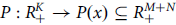$$P:R_ + ^K \to P\left( x \right) \subseteq R_ + ^{M + N}$$

where the output set $P\left( x \right)$ is the set of all output vectors that could be produced by input vector $x$ . We define and specify variable returns to scale (VRS), which is reasonable for the FCS given the wide range of sizes of the Associations. We allow the technology set to change each quarter and efficiency is measured in reference to that technology set.

To include undesirable outputs into the model, assume that the desirable outputs are strongly disposable, meaning that they can be disposed without cost:

$$\left( {{y_0},{b_0}} \right) \in P\left( x \right)\,{\rm{and}}\,\left( {y,{b_0}} \right) \le \left( {{y_0},{b_0}} \right) \Rightarrow \left( {y,{b_0}} \right) \in P\left( x \right),$$

while the undesirable outputs, in addition to the desirable outputs, are weakly disposable, which implies that disposing of them is not free:

$$\left( {y,b} \right) \in P\left( x \right)\,{\rm{and}}\,0 \le \theta \le 1 \Rightarrow \left( {\theta y,\theta b} \right) \in P\left( x \right).$$

This model also assumes null-jointness in desirable and undesirable outputs:

$$\left( {y,b} \right) \in P\left( x \right),\,{\rm{and}}\,b \ =0 \Rightarrow \,y=\,0.$$

“Null-jointness” was introduced by Shephard and Färe (Reference Shephard, Färe, Eichhorn, Henn, Opitz and Shephard1974), meaning that if no bad outputs are produced, there can be no good outputs produced. Alternatively, if one wishes to produce some good outputs, then there will be undesirable by-products, although reducing undesirables will increase efficiency. In our case, the “null-jointness” assumption requires that at least one of the ACAs has non-negative NPLs in the production possibility set, which is met in the data.

With the specified assumptions above, the DDF-based SBM for each decision-making unit (DMU) “ $o$ ” for each time period can be written as follows.

(1) $${\alpha _o} = \mathop {\max }\limits_{\left\{ {\gamma ,\mu ,\phi ,z} \right\}} \left\{ {{\gamma _1} + \ldots + {\gamma _M} + {\mu _1} + \ldots + {\mu _N} + {\phi _1} + \ldots + {\phi _k}} \right\}$$

Subject to

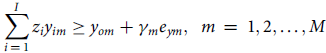$$\mathop \sum \limits_{i\,=\,1}^I {z_i}{y_{im}} \ge {y_{om}} + {\gamma _m}{e_{ym}},{\rm{\;\;}}m\,=\,1,2, \ldots ,M$$

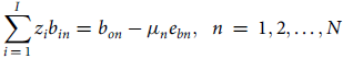$$\mathop \sum \limits_{i\,=\,1}^I {z_i}{b_{in}} = {b_{on}} - {\mu _n}{e_{bn}},{\rm{\;\;}}n\,=\,1,2, \ldots ,N$$

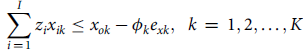$$\mathop \sum \limits_{i\,=\,1}^I {z_i}{x_{ik}} \le {x_{ok}} - {\phi _k}{e_{xk}},{\rm{\;\;}}k\,=\,1,2, \ldots ,K$$

$${z_i} \ge 0,{\rm{\;}}\mathop \sum \limits_{i\,=\,1}^I {z_i}\,=\,1,{\rm{\;\;}}i\,=\,1, \ldots ,I$$

$${\gamma _m} \ge 0,{\mu _n} \ge 0,{\phi _k} \ge 0,{\rm{\;\;}}m\,=\,1, \ldots ,M;n\,=\,1, \ldots ,N;k\,=\,1, \ldots ,K,$$

where $\gamma = \left( {{\gamma _1}, \ldots ,{\gamma _M}} \right)$ , $\;\mu = \left( {{\mu _1}, \ldots ,{\mu _N}} \right)$ , and $\;\phi = \left( {{\phi _1}, \ldots ,{\phi _K}} \right)$ represent the number of units (one dollar in this case) by which outputs can be expanded, and inputs can be reduced to reach the production frontier. Variables ${y_{om}}$ , ${b_{on}}$ , and ${x_{ok}}$ are the $m$ th desirable output, the $n$ th undesirable output, and the $k$ th input of firm $o$ , respectively. The ${z_i}$ , $i\,=\,1, \ldots ,I$ are the intensity variables of DMU $i$ which permit the construction of convex combinations of outputs and inputs. The assumption of VRS is imposed by the constraint $\mathop \sum \nolimits_{i\,=\,1}^I {z_i}\,=\,1$ .

The vector $e = ({e_y}$ , ${e_b}$ , ${e_x}) = \left( {{e_1},\; \ldots ,\;{e_m},\;{e_{m+1}},\; \ldots ,\;{e_{m + n}},\;{e_{m + n+1}},\; \ldots ,{e_{m + n + k}}} \right) \ne 0$ is defined as the directional vector. This model expands desirable outputs and contracts inputs and undesirable outputs. There are usually two ways to define directional vectors. One is to set $e = ({e_y}$ , ${e_b}$ , ${e_x}) = \left( {1,\;1,\;1} \right)$ and interpret the solution values $e\;$ as the net improvement in terms of feasible increase in good outputs and feasible decreases in bad outputs and inputs. The other is to define the direction based on the observed data, that is, $e = ({e_y}$ , ${e_b}$ , ${e_x}) = \left( {{y_o},{b_o},{x_o}} \right)$ , and hence the interpretation of $e$ is the potential proportionate expansion in desirable outputs and contraction in undesirable outputs and inputs. Here we set $\;e = ({e_y}$ , ${e_b}$ , ${e_x}) = \left( {1,\;1,\;1} \right)$ . To impose the weak disposability assumption on the undesirable outputs, equality is specified in the constraint for the contraction of the undesirable outputs.

Data

Data were obtained from quarterly Call Reports collected by the FCA.Footnote ² Every institution of the FCS is required to provide uniform reports of financial conditions and performance on the last day of each calendar quarter. These Call Report quarterly data are available from December 1984. However, for analyzing the outputs with more details and more precision, we use data from the first quarter of 2005, when the loan amounts began to be reported by differentiated loan type, to the first quarter of 2020 (March 2020), which provides information from 61 quarters over the past 15 years. We focus on the ACAs. Although agricultural conditions vary from region to region, all ACAs are subject to the same financial standards. This means the reports have the same financial structure and are comparable across Associations.

There are two main data approaches in the banking efficiency literature: the “production” approach and the “intermediation” approach. The production approach considers financial institutions as primarily producing services for account holders. In the intermediate approach, financial institutions are primarily viewed as intermediating funds between savers and investors (Berger and Humphrey Reference Berger and Humphrey1997). We used the intermediation approach because the role of the Associations is the intermediation process of funds between savers (security holders) and borrowers.

Based on the intermediation approach, we could use the service flow data or the stock of financial value in the accounts. The former corresponds to the income sheet of accounting statements, such as the interest and noninterest incomes and expenses. The latter corresponds to the balance sheet of accounting statements, such as loans and deposits (Berger and Humphrey Reference Berger and Humphrey1991). We choose to use the service flow data, because it more correctly represents the flow of inputs and outputs in a production framework, although few papers do because service flow data are not usually available. Service flow data are available because the Call Reports of accounting statements of the FCA include income flows such as interest income from various assets and expenditures.

We treat the interest expense as a single variable input but differentiate the noninterest expense into three inputs: employee and director salaries (labor), occupancy and equipment expense (capital), and other noninterest expense. This results in four defined inputs: interest, labor, capital, and other noninterest expenses.

Desirable outputs (good outputs) are interest income and noninterest income. The loans made directly to agriculture are the dominant loan type, so we separate the loan interest from the total interest income first and then differentiate it by three loan types: agricultural production, agribusiness, and other.

Unfortunately, although loan amounts on the balance sheet are differentiated by loan type, loan interest by loan type is not reported. Interest income is simply reported as total interest from loans. Thus, to generate loan interest by loan type, the total interest income reported by an Association is allocated across the loan types by the proportion of each type of loan (i.e., agricultural production, agribusiness, and others) to total loans. This assumes that the interest rate is identical across loan types. The alternative would be to use loan values rather than interest as outputs, which would lead to the same empirical results. Noninterest income is another variable in the set of total desirable outputs. This results in four desirable outputs: interest income from agricultural production loans, interest income from agribusiness loans, interest income from other loans, and noninterest income.

The definition of NPLs varies across articles. Usually, articles include some or all following terms: bankrupt loans (loans to borrowers in legal bankruptcy and past-due loans by 6 months or more), restructured loans (the sum of past-due loans by 3 months but less than 6 months and restructured loans), substandard loans, and doubtful assets (Fukuyama and Weber Reference Fukuyama and Weber2008; Fukuyama and Weber Reference Fukuyama and Weber2009; Barros et al. Reference Barros, Managi and Matousek2012; Huang et al. Reference Huang, Chen and Yin2014; Mamatzakis et al. Reference Mamatzakis, Matousek and Vu2016).

We define the loan charge-offs, the allowance for losses charged-off on loans,Footnote ³ as the NPLs, and thus an undesirable output. Although our choice is different from other papers, we argue that the charge-offs can be a reasonable proxy of NPLs. The first and most important reason is that charge-offs in the Call Reports are differentiated by loan types. To be specific, we have three types of charge-offs: charge-off from agricultural production, charge-off from agribusiness, and other charge-offs, which are consistent with our loan types. Loan charge-offs differentiated by loan types allow us to understand the source of the bad loans and measure their separate impact on inefficiencies. In contrast, loan losses usually defined as undesirable output in other papers are not differentiated by loan type. Second, the definition of “loan charge-offs” in the instruction to complete the Call Report states,Footnote ⁴ “loans that determined to be uncollectible and charged off from the allowance for losses during the period.” Charge-offs are, therefore, considered uncollectible loans, and Associations must use their allowance to write off or “pay” for these losses. This implies the charge-offs indeed cause damage to the Associations, at least in that specific period. Although charge-offs might be recovered in the future, the influence on efficiency in a specific period no doubt exists, and the recovery rate of charge-offs, may be very low.

Loans that might be problematic but before being charged-off are loans past due. If the loan status is “past due 30 through 89 days,” or even “past due 90 days or more,” then this loan might be at higher risk and may become bad loans eventually. However, data on this type of problematic loan are only available for a few Associations in our sample and comprise a very small portion of all loans, so we do not include this type of problem loans into the undesirable output set.

Summary statistics for the first and last periods are reported in Table 1. The number of ACAs held mostly steady at 81 from year 2005 through year 2010 and then gradually decreased to 65 Association through mergers and consolidations by year 2020. The number of ACAs decreased over the past 15 years, while all the statistics of input and output variables increased over time. This implies the average size of the Associations increased.

Table 1.

Summary statistics of ACAs of the Farm Credit System (1,000 USD)

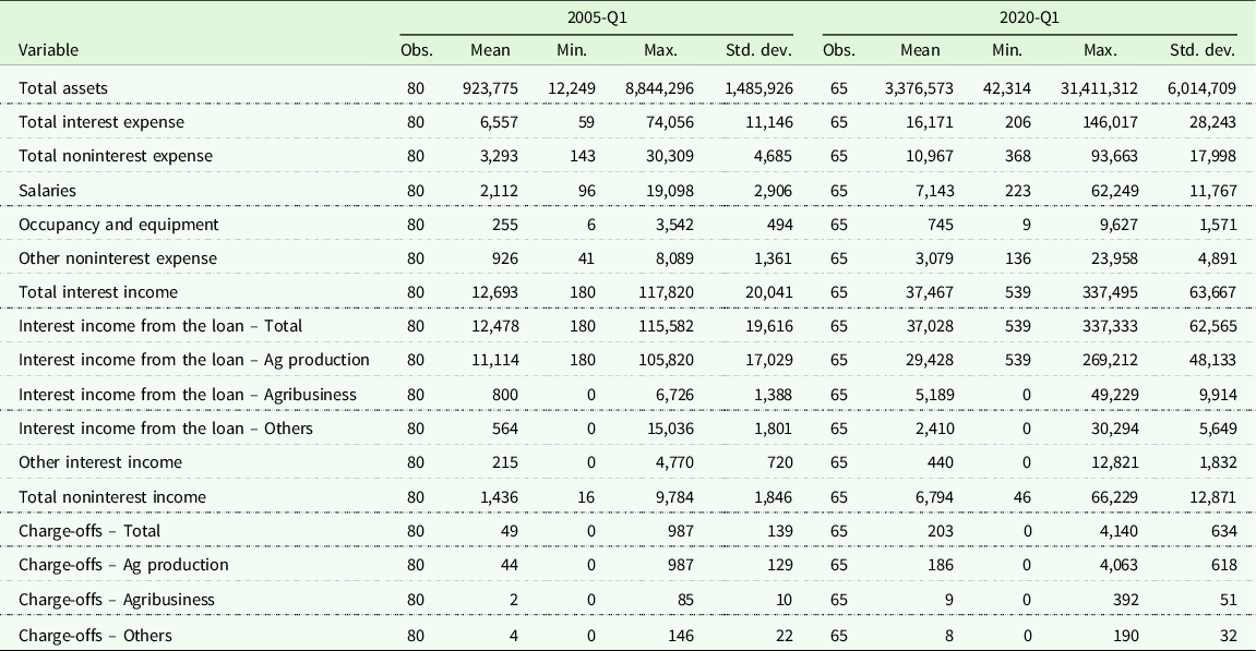
Note: We report the first and the last quarters in this table. All dollar amounts reported here are in thousands of dollars. The observation in the data in the first quarter of 2005 and 2020 should be 81 and 65, respectively. However, we drop two observations because there are negative numbers in a monetary variable (other noninterest expense).

Figure 1 summarizes the changing trends of mean incomes, expenses, and charge-offs over all quarters. The interest income and interest expense are large components of total income and expense. Both went through a deterioration then recovery over 2008–2015, but this was because of lower market interest rates instead of smaller quantity of loans and bond participation over that period. In contrast, even with the low interest rate, charge-offs were significantly higher from 2008 to 2015 compared to the other years over this period, which is a notable forecast of the deterioration in the calculated efficiency shown in the result section. We also observe that the noninterest income and expense fluctuate periodically, but the apexes always occur in the last quarter of each year. We infer that this is because of activities that occur during the last quarter of each year, such as possible bonuses for employees and other yearend expenses. Overall, the quantity of each type of income and expense increased over time.

Figure 1.

Mean income, expense, and charge-offs of Agricultural Credit Associations of the Farm Credit System by quarter. The line for mean charge-offs of all the ACAs through the quarters is relative to the left y-axis. The other four lines are interest, noninterest incomes, and expenses, which are relative to the right y-axis.

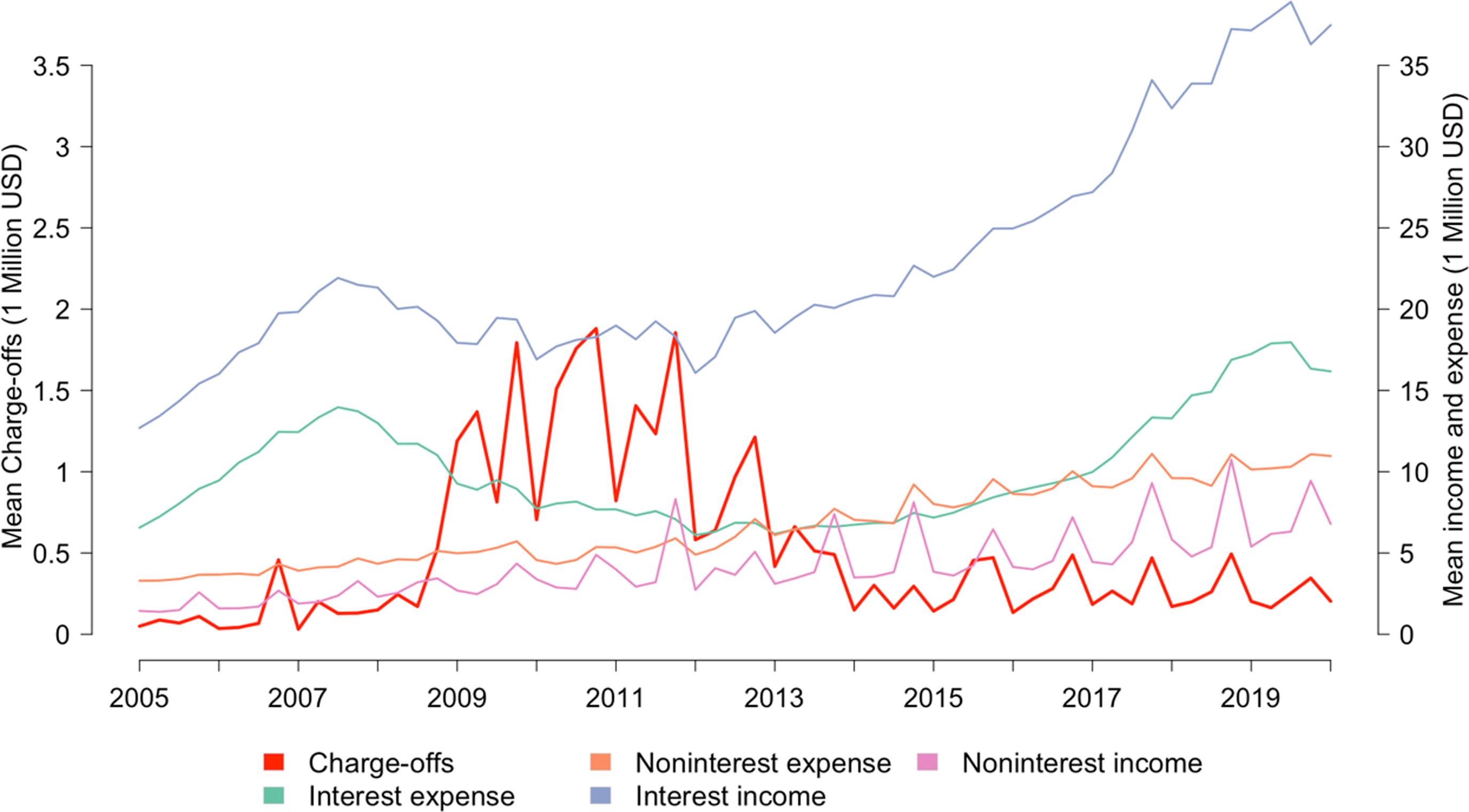
Figure 2 shows the distribution of charges-offs differentiated by loan type in more detail. It is clear that agricultural production accounted for the largest proportion of total loans as well as charge-offs. We can also observe the loan losses went through a dramatic increase during 2008–2015.

Figure 2.

Charge-offs by loan type by ACA of the Farm Credit System. In each boxplot, the top and bottom tails of the box are the maximum and minimum, respectively; the top and bottom edges of the box are the first and third quantiles, respectively. The line in the middle of the box is the median. The y-axis scales are different between the top and bottom graphs.

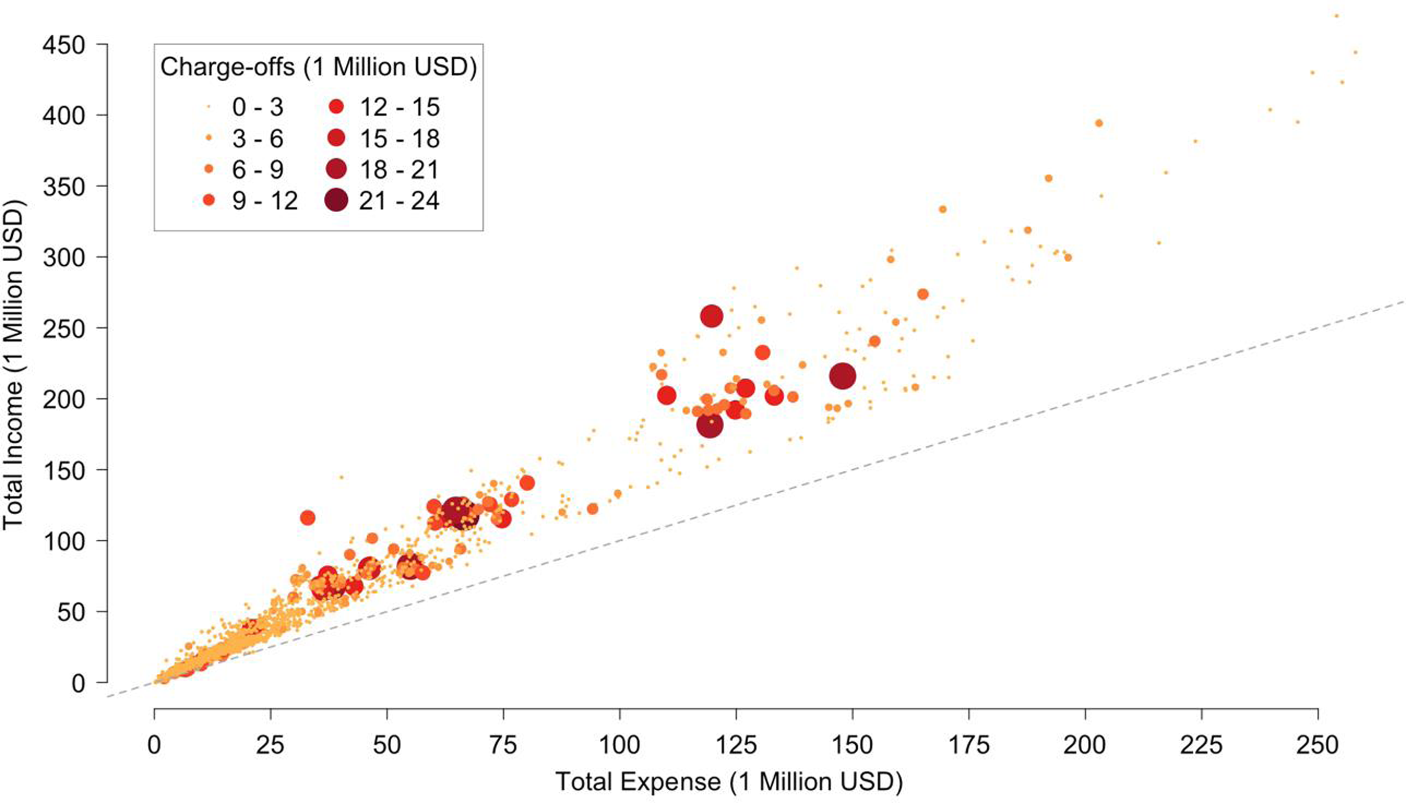
An interesting finding is that larger loan losses are more likely to occur in Associations of small to medium size instead of large size (Figure 3). This might be because larger Associations have better management to monitor loans as well as clients with better ability to repay loans. Figure 3 also shows that as the expenses increase, receipts track above expenses (the 45-degree line as reference). This might imply the return to scale is not constant, which supports the VRS assumption in our model.

Figure 3.

The scale of ACAs of the Farm Credit System and charge-offs. The dashed line is a 45-degree line. Dots above the line represent total receipts greater than total expenses. The larger and darker solid dots represent larger loan losses.

Empirical results

We measure technical efficiencies with NPLs of all the ACAs each quarter from the first quarter of 2005 through the first quarter of 2020 using the DDF-based SBM model under the assumption of variable return to scale using as the technology set the data from all of the Associations for that quarter.

Slacks-based models are non-radial and cannot directly return expansion or contraction ratios as single value efficiency scores. The objective of these slack-oriented models is to maximize the sum of slacks or distances of individual inputs and outputs from each DMU to the frontier. Previous studies define the sum of the distances as the final efficiency score, which can vary substantially and be difficult to interpret due to the different production scales among the output and inputs. Hence, for results interpretation, we define efficiency scores based on the original understanding of efficiency, that is, the ratio between optimal value and observed value. For overall (revenue) or aggregated inputs, outputs, and undesirable outputs, we define the efficiency scores (ES) as follows:

$${\rm{E}}{{\rm{S}}_{{\rm{overall}}}} = {{{{\rm{observed\;revenue}}}}\over{{{\rm{optimal\;revenue}}}}}$$

$${\rm{E}}{{\rm{S}}_{{\rm{input}}}} ={ {{{\rm{optimal\;input}}}}\over{{{\rm{observed\;input}}}}}$$

$${\rm{E}}{{\rm{S}}_{{\rm{output}}}} = {{{{\rm{observed\;output}}}}\over{{{\rm{optimal\;output}}}}}$$

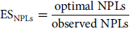$${\rm{E}}{{\rm{S}}_{{\rm{NPLs}}}} = {{{{\rm{optimal\;NPLs}}}}\over{{{\rm{observed\;NPLs}}}}}$$

where “observed” is the actual quantity for each Association, and “optimal” is the quantity that would place that Association on the frontier of the production set. These efficiency scores are bounded over $\left[ {0,1} \right]$ where the value of one represents fully or complete efficient.

The estimation returns disaggregated efficiency scores by input/output/NPL, which is too extensive to individually report in detail.Footnote ⁵ We only show the efficiency by quarter on two aggregated levels: the overall efficiency and the efficiency aggregated over inputs, outputs, or NPLs. We then interpret the summarized results across Associations by period and across periods by Associations, after which we show the results of M&As.

Efficiency scores across ACAs by period

We first summarize the efficiency scores by quarter, listing the mean scores of the Associations and show their change over time. Figure 4 shows the mean of the Associations of the overall efficiency of each period. There was an apparent deterioration in mean efficiency scores over the years 2008–2018, a period of financial difficulties in the US agriculture. Recalling the rising trend of the charge-offs during 2008–2015 shown in Figure 2, we observe an obvious correlation between these patterns. Compared to the fall back of the charge-off quantity in 2015, the recovery of efficiency seems slower, which did not return to the previous level until 2018.

Figure 4.

Overall average efficiency scores of the ACAs of the Farm Credit System. The line is plotted by averaging the point estimation of efficiency score of each Association.

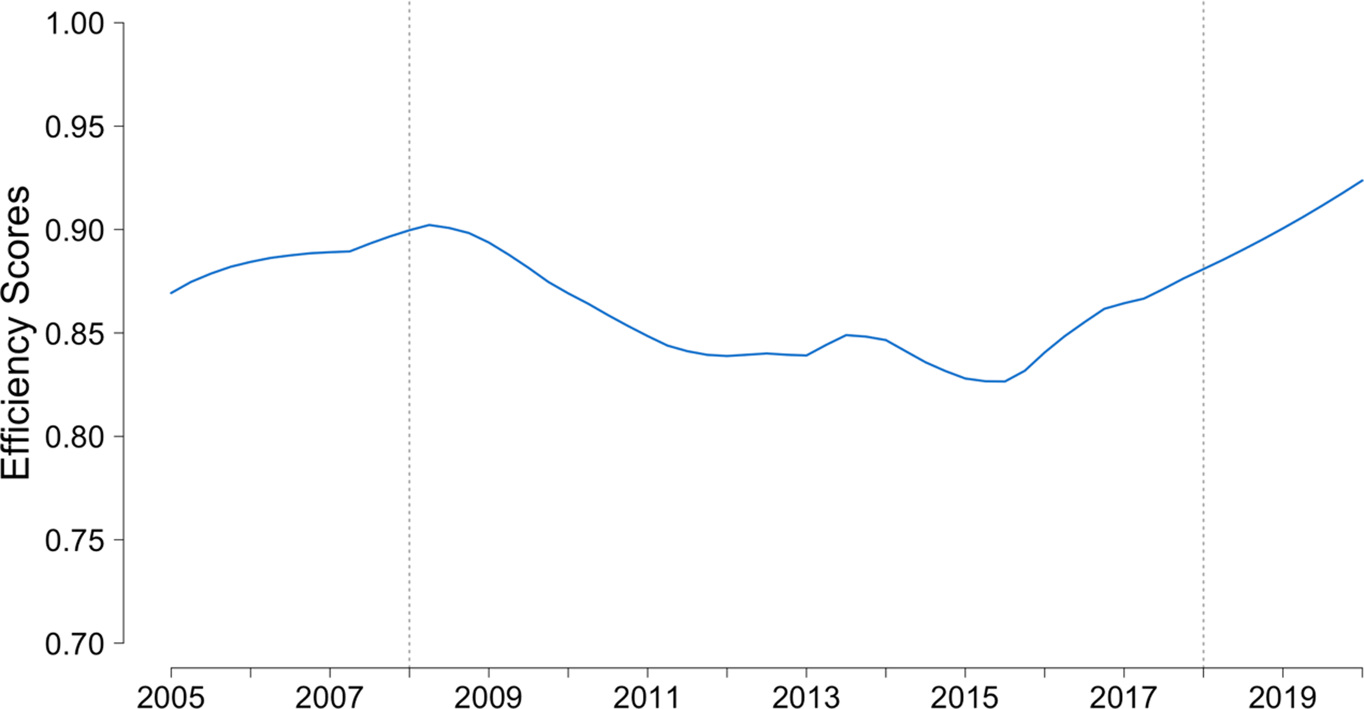
Note, however, the mean efficiency score only reflects the relationship among the Associations in a specific period and under the specific production technology of that period. The decrease in mean efficiency does not necessarily mean the production frontier fell since efficiency is measured relative to the best-managed Associations each period which defines the frontier. The lower the mean, the greater the gaps between the inefficient and efficient Associations. Therefore, the deterioration implies that compared to those Associations on the frontier, which may also have shrunk because of the financial difficulties during those 10 years, other Associations performed even worse.

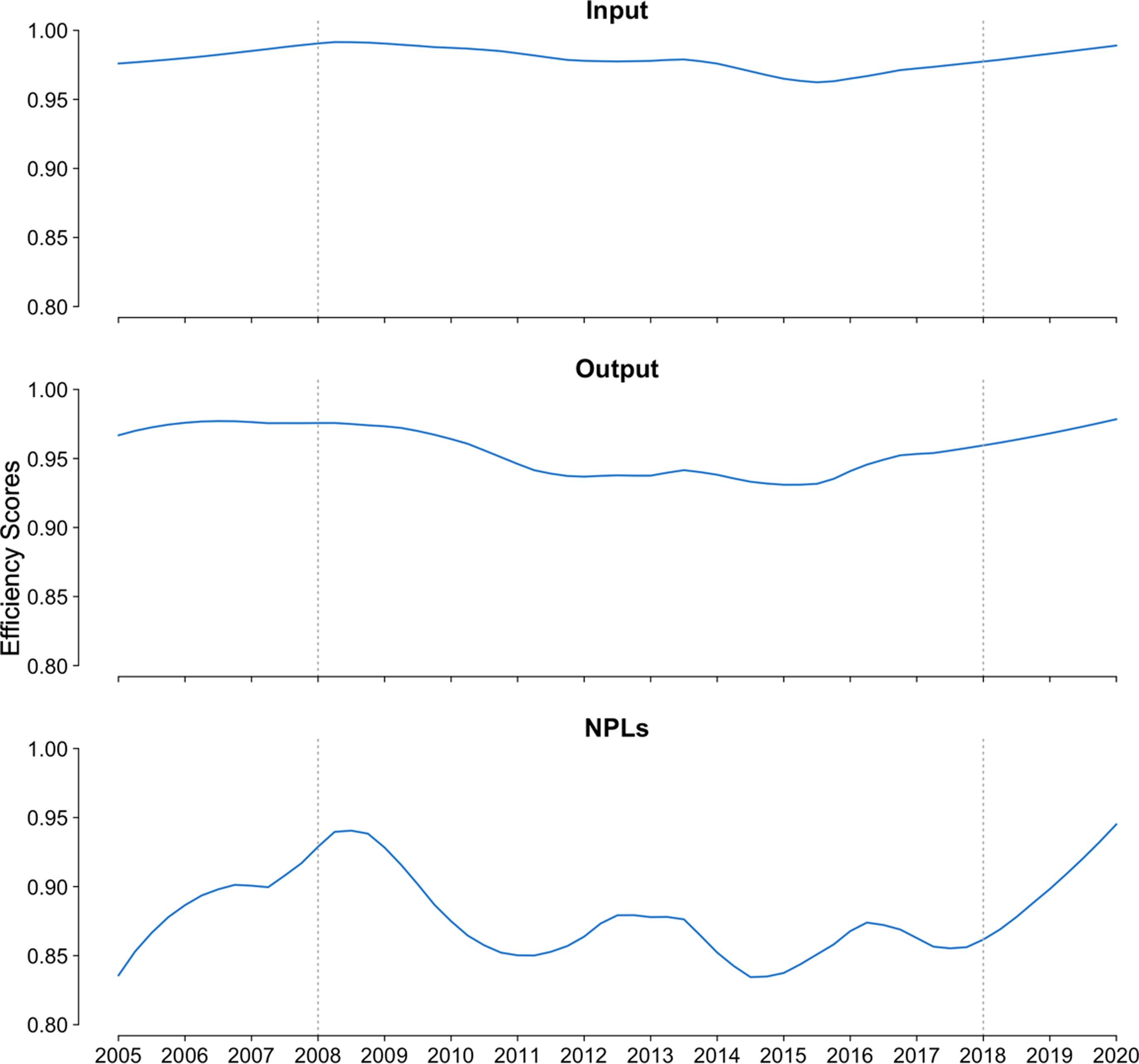
Mean aggregated input, output, and undesirable output efficiencies for each quarter are shown in Figure 5. The input efficiency scores generally remain high, while the average output and undesirable output efficiencies deteriorated during 2008–2018. This implies that when the external environment becomes unfavorable, the management skills to control input effectiveness remain high across Associations, but the management of outputs, including undesirable ones, deteriorated severely for some Associations, widening the gap between efficient and inefficient Associations and leading to decreased average efficiency scores. This is a very different story compared to the history of financial institution merger waves that happened during the 1980s and 1990s, when most of the financial institution managers were seeking to improve input efficiency instead of output efficiency (Broaddus Reference Broaddus1998). The efficiency score of NPLs is lower than both inputs and loan outputs, which implies that the better way of performing well and keeping a higher efficiency is to focus on controlling the NPLs.

Figure 5.

Efficiency scores for aggregated input and output of the ACAs of the Farm Credit System. For each panel, the line is plotted by averaging the point estimation of efficiency score of each Association.

The specific outputs plotted in Figure 6 that lead to the management difficulties can be ascertained by investigating the disaggregated efficiencies. This figure provides an overall sense of which inputs and outputs are generally difficult to manage and can provide managers with information to improve Association performance. For instance, among all kinds of outputs, interest income not from loans (‘Income: other interest’) in Figure 6 has the lowest average efficiency, implying the management skill on this type of output varies across Associations. This may because Associations have greater expertise in making and servicing agricultural and rural loans compared to managing short-term investment funds.

Figure 6.

Efficiency scores for disaggregated input and output of ACAs of the Farm Credit System. For each panel, the line is plotted by averaging the point estimation of efficiency score of each Association.

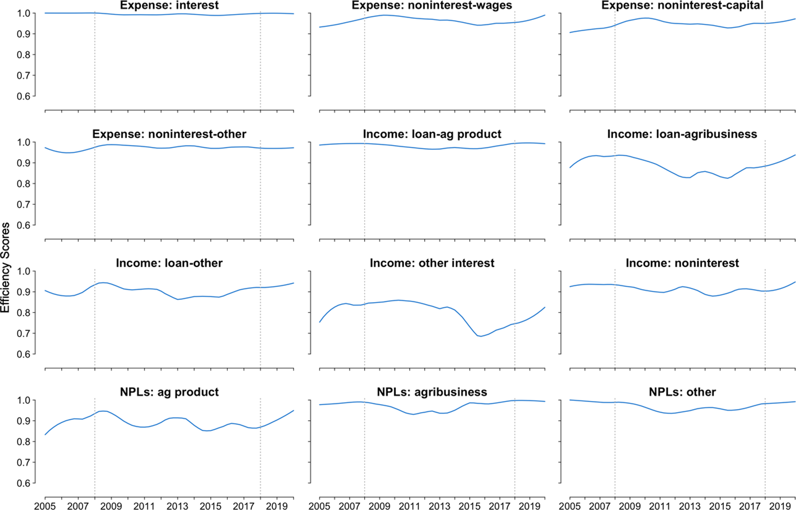
Similarly, the importance of production efficiency of loans for agricultural production, which is the largest loan type and a crucial income source of ACAs, is also shown in Figure 6. The average efficiency of this loan production is relatively high, but its corresponding NPLs efficiency is the lowest among the undesirable outputs. This implies that the management skills to make loans for agricultural production are similar across Associations, while some Associations fail to control the NPLs associated with these loans. Interestingly, this pattern is inversed for other types of loans. The ability to manage loan efficiently for agribusiness and other loans varies across Associations, while the control of their NPLs is quite similar. This may because compared to loans for agricultural production, loans for other purposes are a smaller component of the loan portfolio and possibly easier to monitor and control.

Efficiency with M&A

Efficiency variability and size of an Association are often associated with its continuity. We define Association size as the mean of quarterly reported total assets and illustrate efficiency by the mean and standard deviation of efficiency scores of each Association over time. Figure 7 shows the relationship among the size, efficiency, and M&A activities of all ACAs over the past 15 years.

Figure 7.

Size, efficiency, and M&A of ACAs of the Farm Credit System. Assets refer to the mean of quarterly reported total assets. The solid dot’s position (assets and mean efficiency scores) and size (standard deviation of efficiency scores) refer to the scale and performance of the Association. The color of each solid dot reflects the continuity of the Association (whether M&A or continuing). Red solid dots imply that M&A or amend never happened to such Associations; green solid dots refer to the Associations that take M&A or amend strategies; and the blue ones are merged or amended to other Associations (green). ${10^5}\;$ thousand is 1 billion; ${10^{6.5}}$ thousand is about 32 billion.

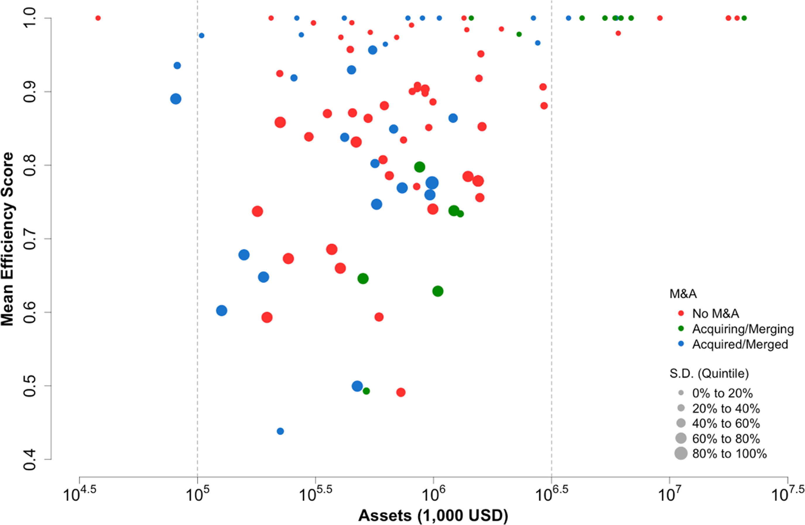
Each solid dot in Figure 7 represents an Association. The position is determined by its size and mean efficiency scores, and the diameter (standard deviation of efficiency scores) refers to the variation of efficiency over time. The color of each solid dot reflects the continuity of the Association: whether the Association was merged or acquired into another Association or continued with no M&A activity. Red solid dots indicate that neither merger nor acquisition ever happened to that Association, green refers to the acquiring Association, and blue indicates the target Association.

If the mean efficiency score of an Association is high and the standard deviation is low, it performed well all the time (small solid dots at the top of Figure 7); while if the mean efficiency score of an Association is low while the standard deviation is high, then this Association’s performance varied over time (big solid dots at the bottom of Figure 7). The bigger the dot, the more volatile the Association’s performance is.

Most Associations have total assets between $1 billion and $32 billion. There are few Associations with total assets less than $1 billion. Most of these small Associations merged in the earlier periods and hence stopped reporting FCA Call Report (blue solid dots), except for Delta (the red solid dot at the up-left corner in Figure 7). Many medium-sized Associations never went through an M&A process. Others did not perform well and hence merged into other, usually larger, Associations (blue from the left to green at the right). Only a few of these medium-sized Associations were constantly efficient. When Associations reach large scales beyond $32 billion, they are almost always efficient and define the production frontier. These Associations gather at the upper-right corner of Figure 7.

Efficiency results for Associations divided into the three groups based upon continuity (no M&A, merger, and acquisition) are shown in Tables 2–4. Table 2 shows the aggregated efficiencies in the first quarter of every other year of the representative Associations that never experienced an M&A activity. Some Associations always perform well and are on the frontier no matter whether large in size (e.g., Farm Credit Mid-America) or small in size (e.g., Delta). Some Associations increased in efficiency over time, such as AgPreference, while others became less efficient over time, such as Legacy Ag Credit. Northwest Florida performed poorly during 2010–2014 and then returned to the frontier (began efficient), while Midsouth improved from 2008 to 2012 and then experienced decreased efficiency. Some poor performance periods for a usually well-performed Association might be associated with an increase in NPLs. Northwest Florida is an example.

Table 2.

Efficiency of selected continuing ACAs of the Farm Credit System that never merged with nor acquired another association

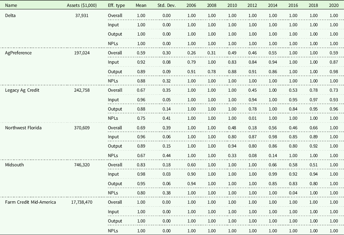
Note: Assets refer to the mean of total assets over the periods that a specific Association exists.

Table 3.

Efficiency of ACAs of the Farm Credit System before and after merging into a new association (Consolidation)

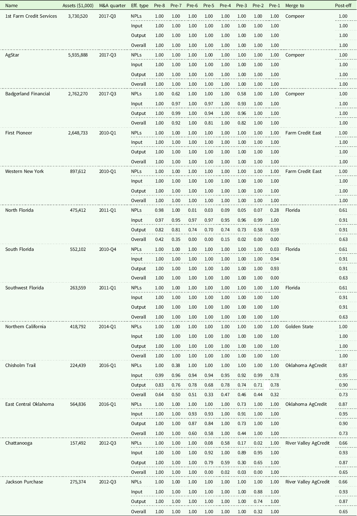
Note: Assets refer to the mean of total assets over the periods that a specific Association exists. The reason why there was only one ACA (Northern California) that was merged into Golden States was because another merger was the Federal Land Bank Association of Kingsburg, FLCA. It did not belong to ACAs and hence was not included into our analysis.

Table 4.

Efficiency of ACAs of the Farm Credit System before and after being acquired by another association

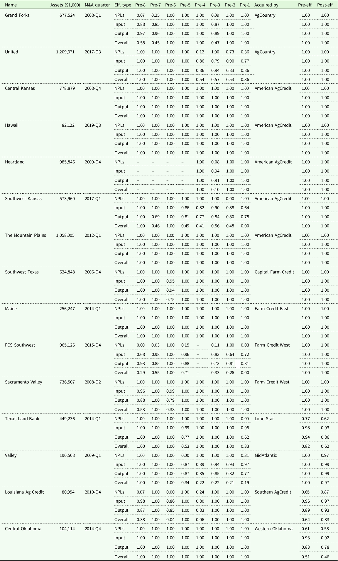
Note: Assets refer to the mean of total assets over the periods that a specific Association exists. AgTexas FCS and Texas Farm Credit Services were also acquired, but not by ACAs. Hence, we did not include them into this table.

Table 3 shows the efficiencies eight quarters (2 years) before Associations merged collectively into a new Association with a name change, with the post-merger efficiency of the new Association. For example, in the third quarter of 2017, three Associations, 1^st Farm Credit Services, AgStar, and Badgerland Financial, merged into a new Association called “Compeer.” Hopefully, the merger process brought the new Association, which is larger than the merged Associations, to a higher performance position, that is, a higher efficiency. However, the actual situations are more complex. For the Compeer example, except for the Badgerland Financial, the other two Associations were originally on the production frontier before the merger. Compeer remained efficient since its formation. We can then infer that this merger helped Badgerland Financial improve its management performance. However, there are also examples where the efficiencies of new Associations did not improve compared to the pre-merger periods. Florida, Oklahoma AgCredit, as well as River Valley AgCredit are examples of such cases. Looking closer at the efficiency scores in the pre-merger periods, some of the former Associations performed much better than others. Not surprisingly, the new Associations performed better than the worst former Association but worse than the best former Association.

Different from merger, another activity often conducted by large Associations is acquisition. Large Associations can expand their scale of operation further through this action. Table 4 shows the efficiencies eight quarters (2 years) before an Association was acquired by another Association, and the average efficiencies of the Associations that conducted the Association pre- and post-periods. Notice that compared to a merger, the Associations that conducted an acquisition were usually more stable and were always on the frontier no matter the performance of the target Association. For instance, AgCountry, American AgCredit, and Capital Farm Credit are examples among others. There are of course exceptional cases whose efficiency scores dropped after the acquisition. Lone Star, MidAtlantic, as well as Western Oklahoma are examples.

Generally, the performance after acquisition seems better than performance with mergers. This might be because the acquisition conducted by large Associations can help improve the performance of the acquired smaller Associations if larger Associations have higher management skills and have more resources to deal with short-run difficulties that might financially challenge smaller Associations; while the merger usually happens among several Associations of similar size, and their combination is a simple expansion of scale, management skill might not experience any improvement during the merger process. Still, as stated before, acquisition does not guarantee a better result. Associations could be less efficient after acquiring others, even though the Associations that were acquired seemed efficient before the acquisition. This shows that some Associations were able to successfully subsume an Association regardless of the efficiency of the assumed Association, while other Associations were not able to accomplish an effective transition with the same success even if the assumed Association was efficient.

Summary and conclusion

The SBM based on DDF was used to evaluate the production efficiency of US ACAs over the period 2005–2020, which allowed efficiency measurement by specified outputs and inputs. Compared to previous studies of the US FCS efficiency measurement, which ignored NPLs, we calculate with NPLs included.

Efficiency scores of inputs are steady and higher than that of outputs, implying that the management skills required to control and monitor inputs are high and similar across Associations, while controlling and monitoring of both good and bad outputs varied considerably, especially during financial difficulties over the period 2008 through 2018.

We analyzed the efficiency scores across time by Association and disentangle the relationship between the size and continuity of each Association. We find that the size and production efficiency of an Association are associated with its continuity, through mergers and acquisitions. The Associations with large total assets (more than $32 billion) always perform very efficiently and thus operate on the production frontier. Associations with large total assets are more likely to acquire other Associations. Associations of medium size are not consistent in their performance, sometimes experiencing higher efficiency scores, at other times lower scores. This might be why some merged with other Associations or were acquired by larger Associations. We analyze the M&A behaviors by showing the sizes and efficiencies of corresponding representative Associations before and after the activity. We find that the M&A process can, to some extent, help small Associations survive and solve short-run difficulties. There was also a chance that the M&A might cause larger accepting Associations to experience a decrease in efficiency after the acquisition.

To conclude, this research calculated the production efficiencies of the ACAs of the FCS with NPLs modeled as an undesirable output. Although many relationships were uncovered and results were discovered, there is still much to explore. For example, we observed a distinct correlation between undesirable outputs and performance failure. The inefficiency of the NPLs is correlated with M&A behavior. However, we did not investigate the causal relationship. Another exploration could be measuring productivity change over time and decomposing into efficiency and technological change.