


1 Exponential valuations
By a polytope
 $P\subset \mathbb R^n$
, we mean the convex hull of finitely many points of
$P\subset \mathbb R^n$
, we mean the convex hull of finitely many points of
 $\mathbb R^n$
. The polytope P is called a segment if
$\mathbb R^n$
. The polytope P is called a segment if
 $\mathrm {dim}\,P=1$
, and P is called a polygon if
$\mathrm {dim}\,P=1$
, and P is called a polygon if
 $\mathrm {dim}\,P=2$
. Let
$\mathrm {dim}\,P=2$
. Let
 $\mathcal {F}$
be a family of compact convex sets in
$\mathcal {F}$
be a family of compact convex sets in
 $\mathbb R^n$
such that if
$\mathbb R^n$
such that if
 $P\cup Q$
is convex for
$P\cup Q$
is convex for
 $P,Q\in \mathcal {F}$
, then
$P,Q\in \mathcal {F}$
, then
 $P\cup Q\in \mathcal {F}$
and
$P\cup Q\in \mathcal {F}$
and
 $P\cap Q\in \mathcal {F}$
. Examples of such families are the family
$P\cap Q\in \mathcal {F}$
. Examples of such families are the family
 $\mathcal {K}^n$
of all convex compact sets in
$\mathcal {K}^n$
of all convex compact sets in
 $\mathbb R^n$
, the family
$\mathbb R^n$
, the family
 $\mathcal {P}^n$
of all polytopes in
$\mathcal {P}^n$
of all polytopes in
 $\mathbb R^n$
and the family
$\mathbb R^n$
and the family
 $\mathcal {P}(\mathbb Z^n)$
of all lattice polytopes; namely, convex hulls of finitely many points of
$\mathcal {P}(\mathbb Z^n)$
of all lattice polytopes; namely, convex hulls of finitely many points of
 $\mathbb Z^n$
(see McMullen [Reference McMullen16]). If
$\mathbb Z^n$
(see McMullen [Reference McMullen16]). If
 $\mathcal {A}$
is a cancellative monoid (cancellative semigroup with identity element
$\mathcal {A}$
is a cancellative monoid (cancellative semigroup with identity element
 $0_{\mathcal {A}}$
), then a function
$0_{\mathcal {A}}$
), then a function
 $Z:\mathcal {F}\to \mathcal {A}$
is called a valuation if the following holds: if
$Z:\mathcal {F}\to \mathcal {A}$
is called a valuation if the following holds: if
 $P\cup Q$
is convex for
$P\cup Q$
is convex for
 $P,Q\in \mathcal {F}$
, then
$P,Q\in \mathcal {F}$
, then
 $$ \begin{align} Z(P\cup Q)+Z(P\cap Q)=Z(P)+Z(Q). \end{align} $$
We say that the valuation
 $Z:\mathcal {F}\to \mathcal {A}$
is simple if
$Z:\mathcal {F}\to \mathcal {A}$
is simple if
 $Z(P)=0_{\mathcal {A}}$
for any
$Z(P)=0_{\mathcal {A}}$
for any
 $P\in \mathcal {F}$
with
$P\in \mathcal {F}$
with
 $\mathrm {dim} P\leq n-1$
. Typically, one would consider valuations intertwining with some natural group actions, as we will shortly see.
$\mathrm {dim} P\leq n-1$
. Typically, one would consider valuations intertwining with some natural group actions, as we will shortly see.
While the idea of valuations on convex polytopes played a crucial role in Dehn’s solution of Hilbert’s third problem already around 1900, after sporadic results, the systematic study of valuations only started with Hadwiger’s celebrated characterization of the intrinsic volumes as the basis of the space of continuous isometry invariant valutions from 1957. For the breathtaking developments of the last seven decades, see, for example, the monograph Alesker [Reference Alesker2], and the survey papers Alesker [Reference Alesker1], Ludwig [Reference Ludwig13] and Ludwig and Mussnig [Reference Ludwig and Mussnig14]. The theory of valuations on lattice polytopes has been flourishing since the classical paper by Betke and Kneser [Reference Betke and Kneser3] in 1985 characterizing unimodular invariant valuations on lattice polytopes (see, e.g., Böröczky and Ludwig [Reference Böröczky and Ludwig4, Reference Böröczky and Ludwig5], Jochemko and Sanyal [Reference Jochemko and Sanyal9, Reference Jochemko and Sanyal10] and Ludwig and Silverstein [Reference Ludwig and Silverstein15]).
To state the result stimulating our research, let
 $L^1_c(\mathbb R^n)$
denote the family of Lebesgue integrable real functions with compact support on
$L^1_c(\mathbb R^n)$
denote the family of Lebesgue integrable real functions with compact support on
 $\mathbb R^n$
. In addition, for measurable
$\mathbb R^n$
. In addition, for measurable
 $\Omega \subset \mathbb R^n$
, let
$\Omega \subset \mathbb R^n$
, let
 $\mathcal {M}(\Omega )$
denote the family of real-valued measurable functions on
$\mathcal {M}(\Omega )$
denote the family of real-valued measurable functions on
 $\Omega $
where measurable means Lebesgue measurable without stating it in this article. Actually, all the arguments and statements in this article apply to the case if we fix a finite dimensional real vector space
$\Omega $
where measurable means Lebesgue measurable without stating it in this article. Actually, all the arguments and statements in this article apply to the case if we fix a finite dimensional real vector space
 $\mathcal {V}$
, and
$\mathcal {V}$
, and
 $\mathcal {M}(\Omega )$
denotes the family of measurable functions
$\mathcal {M}(\Omega )$
denotes the family of measurable functions
 $\Omega \to \mathcal {V}$
, including the case of complex-valued measurable functions. However, for simplicity, we just discuss real-valued functions. For
$\Omega \to \mathcal {V}$
, including the case of complex-valued measurable functions. However, for simplicity, we just discuss real-valued functions. For
 $f\in L^1_c(\mathbb R^n)$
, its Laplace transform is
$f\in L^1_c(\mathbb R^n)$
, its Laplace transform is
 $$ \begin{align*}\mathcal{L}f(x)=\int_{\mathbb R^n}e^{-\langle x,y\rangle}f(y)\,dy. \end{align*} $$
Li andMa [Reference Li and Ma12] extended the definition of the Laplace transform to a convex compact set K by applying
 $\mathcal {L}$
to the characteristic function; namely,
$\mathcal {L}$
to the characteristic function; namely,
 $$ \begin{align*}\mathcal{L}K=\mathcal{L}\mathbf{1}_K=\int_Ke^{-\langle x,y\rangle}\,dy. \end{align*} $$
Inspired by the properties of the Laplace transform applied to the characteristic functions of compact convex sets, Li and Ma [Reference Li and Ma12] considered valuations that are translatively exponential and
 $\mathrm {GL}(n,\mathbb R)$
covariant. For a subgroup
$\mathrm {GL}(n,\mathbb R)$
covariant. For a subgroup
 $G\subset \mathrm {GL}(n,\mathbb R)$
, we say that a valuation
$G\subset \mathrm {GL}(n,\mathbb R)$
, we say that a valuation
 $Z:\mathcal {K}^n\to \mathcal {M}(\mathbb R^n)$
is translatively exponential and G covariant if for any
$Z:\mathcal {K}^n\to \mathcal {M}(\mathbb R^n)$
is translatively exponential and G covariant if for any
 $x\in \mathbb R^n$
, we have
$x\in \mathbb R^n$
, we have
 $$ \begin{align} Z(\Phi K)(x)&=|\det \Phi|\cdot Z( K)(\Phi^Tx) \text{for any } \Phi\in G; \end{align} $$
 $$ \begin{align} Z( K+z)(x)&=e^{-\langle z,x\rangle} Z(K)(x) \text{for any } z\in\mathbb R^n, \end{align} $$
respectively. The Hausdorff distance
 $\delta _H(C,K)$
between compact convex sets
$\delta _H(C,K)$
between compact convex sets
 $K, C\subset \mathbb R^n$
is the minimal
$K, C\subset \mathbb R^n$
is the minimal
 $r\geq 0$
such that
$r\geq 0$
such that
 $K\subset C+r B^n$
and
$K\subset C+r B^n$
and
 $C\subset K+r B^n$
where
$C\subset K+r B^n$
where
 $B^n$
is the unit ball in
$B^n$
is the unit ball in
 $\mathbb R^n$
centered at the origin. We say that a valuation
$\mathbb R^n$
centered at the origin. We say that a valuation
 $Z:\mathcal {K}^n\to \mathcal {M}(\mathbb R^n)$
is continuous if for any convergent sequence
$Z:\mathcal {K}^n\to \mathcal {M}(\mathbb R^n)$
is continuous if for any convergent sequence
 $K_i\to K$
of compact convex sets with respect to the Hausdorff distance,
$K_i\to K$
of compact convex sets with respect to the Hausdorff distance,
 $Z(K_i)$
tends pointwise to
$Z(K_i)$
tends pointwise to
 $Z(K)$
. In addition,
$Z(K)$
. In addition,
 $C(\mathbb R^n)$
denotes the space of real continuous functions on
$C(\mathbb R^n)$
denotes the space of real continuous functions on
 $\mathbb R^n$
.
$\mathbb R^n$
.
Theorem 1 (Li and Ma [Reference Li and Ma12])
Any continuous translatively exponential and
 $\mathrm {GL}(n,\mathbb R)$
covariant valuation
$\mathrm {GL}(n,\mathbb R)$
covariant valuation
 $Z:\mathcal {K}^n\to C(\mathbb R^n)$
is of the form
$Z:\mathcal {K}^n\to C(\mathbb R^n)$
is of the form
 $Z=c\mathcal {L}$
for a constant
$Z=c\mathcal {L}$
for a constant
 $c\in \mathbb R$
.
$c\in \mathbb R$
.
Even if – as we will shortly see – there is an abundance of translatively exponential and
 $\mathrm {GL}(2,\mathbb Z)$
covariant valuations
$\mathrm {GL}(2,\mathbb Z)$
covariant valuations
 $Z:\mathcal {P}(\mathbb Z^2)\to \mathcal {M}(\mathbb R^n)$
on lattice polytopes, we still believe that it is not so for translatively exponential and
$Z:\mathcal {P}(\mathbb Z^2)\to \mathcal {M}(\mathbb R^n)$
on lattice polytopes, we still believe that it is not so for translatively exponential and
 $\mathrm {GL}(n,\mathbb R)$
covariant valuations
$\mathrm {GL}(n,\mathbb R)$
covariant valuations
 $Z:\mathcal {P}^n\to \mathcal {M}(\mathbb R^n)$
on polytopes in
$Z:\mathcal {P}^n\to \mathcal {M}(\mathbb R^n)$
on polytopes in
 $\mathbb R^n$
.
$\mathbb R^n$
.
Conjecture 2 Any translatively exponential and
 $\mathrm {GL}(n,\mathbb R)$
covariant valuation
$\mathrm {GL}(n,\mathbb R)$
covariant valuation
 $Z:\mathcal {P}^n\to \mathcal {M}(\mathbb R^n)$
is of the form
$Z:\mathcal {P}^n\to \mathcal {M}(\mathbb R^n)$
is of the form
 $Z=c\mathcal {L}$
for a constant
$Z=c\mathcal {L}$
for a constant
 $c\in \mathbb R$
(Figure 1).
$c\in \mathbb R$
(Figure 1).
In this article, we consider some valuation Z on lattice polygons (of
 $\mathbb Z^2$
) with values in the space of measurable functions that satisfy (4) and (5): If
$\mathbb Z^2$
) with values in the space of measurable functions that satisfy (4) and (5): If
 $x\in \mathbb R^2$
, then
$x\in \mathbb R^2$
, then
 $$ \begin{align} Z( P+z)(x)&=e^{\langle z,x\rangle} Z( P)(x) \text{for any } z\in\mathbb Z^2; \end{align} $$
 $$ \begin{align} Z(\Phi P)(x)&=Z( P)(\Phi^Tx) \text{for any } \Phi\in \mathrm{GL}(2,\mathbb Z)\end{align} $$
where (5) is a restriction of (2) to
 $\mathrm {GL}(2,\mathbb Z)$
as
$\mathrm {GL}(2,\mathbb Z)$
as
 $|\det \phi |=1$
for
$|\det \phi |=1$
for
 $\Phi \in \mathrm {GL}(2,\mathbb Z)$
. One example is the “positive Laplace transform”
$\Phi \in \mathrm {GL}(2,\mathbb Z)$
. One example is the “positive Laplace transform”
 $$ \begin{align*}\mathcal{L}_+(P)(x)=\int_{\mathbb R^n}e^{\langle x,y\rangle}\mathbf{1}_P(y)\,dy=\int_Pe^{\langle x,y\rangle}\,dy. \end{align*} $$
We observe that
 $x\mapsto Z(P)(x)$
satisfies (4) if and only if
$x\mapsto Z(P)(x)$
satisfies (4) if and only if
 $x\mapsto Z(P)(-x)$
satisfies (3). We note that Freyeret al. [Reference Freyer, Ludwig and Rubey8] characterized the translatively exponential and
$x\mapsto Z(P)(-x)$
satisfies (3). We note that Freyeret al. [Reference Freyer, Ludwig and Rubey8] characterized the translatively exponential and
 $\mathrm {GL}(2,\mathbb Z)$
covariant valuations with values in the space of formal power series in two variables.
$\mathrm {GL}(2,\mathbb Z)$
covariant valuations with values in the space of formal power series in two variables.
The main goal of this article is to characterize translatively exponential and
 $\mathrm {GL}(2,\mathbb Z)$
covariant valuations
$\mathrm {GL}(2,\mathbb Z)$
covariant valuations
 $Z:\mathcal {P}(\mathbb Z^2)\to \mathcal {M}(\mathbb R^2)$
. We write
$Z:\mathcal {P}(\mathbb Z^2)\to \mathcal {M}(\mathbb R^2)$
. We write
 $e_1,e_2$
to denote the orthonormal basis of
$e_1,e_2$
to denote the orthonormal basis of
 $\mathbb R^2$
also generating
$\mathbb R^2$
also generating
 $\mathbb Z^2$
, and set
$\mathbb Z^2$
, and set
 $T=[e_1,e_2,o]$
where
$T=[e_1,e_2,o]$
where
 $o=(0,0)$
stands for the origin, and
$o=(0,0)$
stands for the origin, and
 $[x_1,\ldots ,x_k]$
stands for the convex hull of
$[x_1,\ldots ,x_k]$
stands for the convex hull of
 $x_1,\ldots ,x_k\in \mathbb R^2$
. In the formulas below
$x_1,\ldots ,x_k\in \mathbb R^2$
. In the formulas below
 $$ \begin{align*}\frac{e^t-1}{t}\text{ is identified with }\sum_{n=0}^\infty\frac{t^n}{(n+1)!}; \end{align*} $$
namely, when we write
 $\varphi (t)=\frac {e^t-1}{t}$
, we mean the positive analytic function
$\varphi (t)=\frac {e^t-1}{t}$
, we mean the positive analytic function
 $\varphi (t)=\sum _{n=0}^\infty \frac {t^n}{(n+1)!}$
on
$\varphi (t)=\sum _{n=0}^\infty \frac {t^n}{(n+1)!}$
on
 $\mathbb R$
satisfying
$\mathbb R$
satisfying
 $\varphi (0)=1$
. For the golden ratio
$\varphi (0)=1$
. For the golden ratio
 $\tau =\frac {\sqrt {5}+1}2$
, we set (see Figure 1)
$\tau =\frac {\sqrt {5}+1}2$
, we set (see Figure 1)
 $$ \begin{align*}\widetilde{\Omega}_{2}=\{(\tau s,s):1\leq s<\tau\}\cup \{(x_1,x_2):0\leq x_1\leq x_2\}. \end{align*} $$
The domain
 $\widetilde {\Omega }_2$
.
$\widetilde {\Omega }_2$
.

First, we characterize simple translatively exponential and
 $\mathrm {GL}(2,\mathbb Z)$
covariant valuations where a valuation
$\mathrm {GL}(2,\mathbb Z)$
covariant valuations where a valuation
 $Z:\mathcal {P}(\mathbb Z^2)\to \mathcal {M}(\mathbb R^2)$
is simple if
$Z:\mathcal {P}(\mathbb Z^2)\to \mathcal {M}(\mathbb R^2)$
is simple if
 $Z(P)=0$
for any
$Z(P)=0$
for any
 $P\in \mathcal {P}(\mathbb Z^2)$
with
$P\in \mathcal {P}(\mathbb Z^2)$
with
 $\mathrm {dim}\,P\leq 1 $
(Figure 2).
$\mathrm {dim}\,P\leq 1 $
(Figure 2).
Theorem 3 Simple translatively exponential and
 $\mathrm {GL}(2,\mathbb Z)$
covariant valuations
$\mathrm {GL}(2,\mathbb Z)$
covariant valuations
 $Z:\mathcal {P}(\mathbb Z^2)\to \mathcal {M}(\mathbb R^2)$
are parameterized uniquely by functions in
$Z:\mathcal {P}(\mathbb Z^2)\to \mathcal {M}(\mathbb R^2)$
are parameterized uniquely by functions in
 $\mathcal {M}(\widetilde {\Omega }_{2})$
in the following way.
$\mathcal {M}(\widetilde {\Omega }_{2})$
in the following way.
-
(i) For any measurable function
 $\tilde {\varrho }:\widetilde {\Omega }_{2}\to \mathbb R$
, there exists a unique measurable extension
$\varrho :\,[0,\infty )^2\to \mathbb R$
satisfying
$\tilde {\varrho }=\varrho |_{\widetilde {\Omega }_{2}}$
and (6)for
$$ \begin{align} (2x+y) \varrho(x,y)=(x+y)\varrho(x,x+y)+x \varrho(x+y,x) \end{align} $$
$x,y\geq 0$
, and a unique translatively exponential and
$\mathrm {GL}(2,\mathbb Z)$
covariant simple valuation
$Z:\mathcal {P}(\mathbb Z^2)\to \mathcal {M}(\mathbb R^2)$
such that
$Z(T)(0,0)=\tilde {\varrho }(0,0)$
, and
$f_2=Z(T)$
satisfies (7)for
$$ \begin{align} f_2(x,y)=\frac{e^x}{y}\cdot \frac{e^{y-x}-1}{y-x}\cdot \varrho(y-x,x)- \frac{1}y\cdot \frac{e^{x}-1}{x}\cdot \varrho(x,y-x) \end{align} $$
$0\leq x\leq y$
and
$y>0$
.
$\tilde {\varrho }:\widetilde {\Omega }_{2}\to \mathbb R$
, there exists a unique measurable extension
$\varrho :\,[0,\infty )^2\to \mathbb R$
satisfying
$\tilde {\varrho }=\varrho |_{\widetilde {\Omega }_{2}}$
and (6)for
$$ \begin{align} (2x+y) \varrho(x,y)=(x+y)\varrho(x,x+y)+x \varrho(x+y,x) \end{align} $$
$x,y\geq 0$
, and a unique translatively exponential and
$\mathrm {GL}(2,\mathbb Z)$
covariant simple valuation
$Z:\mathcal {P}(\mathbb Z^2)\to \mathcal {M}(\mathbb R^2)$
such that
$Z(T)(0,0)=\tilde {\varrho }(0,0)$
, and
$f_2=Z(T)$
satisfies (7)for
$$ \begin{align} f_2(x,y)=\frac{e^x}{y}\cdot \frac{e^{y-x}-1}{y-x}\cdot \varrho(y-x,x)- \frac{1}y\cdot \frac{e^{x}-1}{x}\cdot \varrho(x,y-x) \end{align} $$
$0\leq x\leq y$
and
$y>0$
.
-
(ii) For any simple translatively exponential and
$\mathrm {GL}(2,\mathbb Z)$
covariant valuation
${Z:\mathcal {P}(\mathbb Z^2)\to \mathcal {M}(\mathbb R^2)}$
, there exists some measurable
$\varrho :\,[0,\infty )^2\to \mathbb R$
satisfying (6) and (7).


Remark. The “positive Laplace transform”
 $\mathcal {L}_+$
corresponds to the constant one function
$\mathcal {L}_+$
corresponds to the constant one function
 $\varrho \equiv 1$
. On the other hand, Freyeret al. [Reference Freyer, Ludwig and Rubey8] determined all translatively exponential and
$\varrho \equiv 1$
. On the other hand, Freyeret al. [Reference Freyer, Ludwig and Rubey8] determined all translatively exponential and
 $\mathrm {GL}(2,\mathbb Z)$
covariant valuations with values in the space of formal power series in two variables. It follows that there exists an abundance of corresponding simple valuations with values in the space of analytic functions that are different from the positive Laplace transform, and we exhibit one in Example 15.
$\mathrm {GL}(2,\mathbb Z)$
covariant valuations with values in the space of formal power series in two variables. It follows that there exists an abundance of corresponding simple valuations with values in the space of analytic functions that are different from the positive Laplace transform, and we exhibit one in Example 15.
We write
 $|X|$
to denote the Lebesgue measure of a measurable set
$|X|$
to denote the Lebesgue measure of a measurable set
 $X\subset \mathbb R^2$
. We need the following consequence of the fact that the linear action of
$X\subset \mathbb R^2$
. We need the following consequence of the fact that the linear action of
 $\mathrm {SL}(2,\mathbb Z)$
on
$\mathrm {SL}(2,\mathbb Z)$
on
 $\mathbb R^2$
is ergodic (see Section 5). Proposition 4 about Lebesgue measurable
$\mathbb R^2$
is ergodic (see Section 5). Proposition 4 about Lebesgue measurable
 $\mathrm {SL}(2,\mathbb Z)$
invariant functions is used in the statement of Theorem 5 characterizing translatively exponential and
$\mathrm {SL}(2,\mathbb Z)$
invariant functions is used in the statement of Theorem 5 characterizing translatively exponential and
 $\mathrm {GL}(2,\mathbb Z)$
covariant valuations.
$\mathrm {GL}(2,\mathbb Z)$
covariant valuations.
Proposition 4 If
 $f\in \mathcal {M}(\mathbb R^2)$
is invariant under
$f\in \mathcal {M}(\mathbb R^2)$
is invariant under
 $\mathrm {SL}(2,\mathbb Z)$
, then there exists a constant
$\mathrm {SL}(2,\mathbb Z)$
, then there exists a constant
 $c\in \mathbb R$
such that
$c\in \mathbb R$
such that
 $f(x)=c$
for almost everywhere
$f(x)=c$
for almost everywhere
 $x\in \mathbb R^2$
.
$x\in \mathbb R^2$
.
Remark. In particular, any function
 $f\in \mathcal {M}(\mathbb R^2)$
invariant under
$f\in \mathcal {M}(\mathbb R^2)$
invariant under
 $\mathrm {GL}(2,\mathbb Z)$
can be constructed in the following way from a
$\mathrm {GL}(2,\mathbb Z)$
can be constructed in the following way from a
 $c\in \mathbb R$
and an
$c\in \mathbb R$
and an
 $X\subset \mathbb R^2$
with
$X\subset \mathbb R^2$
with
 $|X|=0$
. Writing
$|X|=0$
. Writing
 $X_0$
to denote the image of X under the action of
$X_0$
to denote the image of X under the action of
 $\mathrm {GL}(2,\mathbb Z)$
, we have
$\mathrm {GL}(2,\mathbb Z)$
, we have
 $|X_0|=0$
, and associating an arbitrary
$|X_0|=0$
, and associating an arbitrary
 $c_{\mathcal {O}}\in \mathbb R$
to any orbit
$c_{\mathcal {O}}\in \mathbb R$
to any orbit
 $\mathcal {O}$
of
$\mathcal {O}$
of
 $\mathrm {GL}(2,\mathbb Z)$
intersecting X, we define
$\mathrm {GL}(2,\mathbb Z)$
intersecting X, we define
 $f(x)=c$
for
$f(x)=c$
for
 $x\in \mathbb R^2\backslash X_0$
, and
$x\in \mathbb R^2\backslash X_0$
, and
 $f(x)=c_{\mathcal {O}}$
if
$f(x)=c_{\mathcal {O}}$
if
 $x\in \mathcal {O}$
for an orbit
$x\in \mathcal {O}$
for an orbit
 $\mathcal {O}$
of
$\mathcal {O}$
of
 $\mathrm {GL}(2,\mathbb Z)$
intersecting X.
$\mathrm {GL}(2,\mathbb Z)$
intersecting X.
In Theorem 5, we use (see Figure 2)
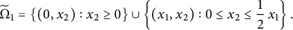 $$ \begin{align*}\widetilde{\Omega}_1=\{(0,x_2):x_2\geq 0\}\cup \left\{(x_1,x_2):0\leq x_2\leq {\frac12\,}x_1\right\}. \end{align*} $$
The domain
 $\widetilde {\Omega }_1$
.
$\widetilde {\Omega }_1$
.

The space of
 $\mathrm {GL}(2,\mathbb Z)$
invariant measurable functions in
$\mathrm {GL}(2,\mathbb Z)$
invariant measurable functions in
 $\mathbb R^2$
– that are characterized in Proposition 4 –, is denoted by
$\mathbb R^2$
– that are characterized in Proposition 4 –, is denoted by
 $\mathcal {M}(\mathbb R^2)^{\mathrm {GL}(2,\mathbb Z)}$
.
$\mathcal {M}(\mathbb R^2)^{\mathrm {GL}(2,\mathbb Z)}$
.
Theorem 5 Translatively exponential and
 $\mathrm {GL}(2,\mathbb Z)$
covariant valuations
$\mathrm {GL}(2,\mathbb Z)$
covariant valuations
 $Z:\mathcal {P}(\mathbb Z^2)\to \mathcal {M}(\mathbb R^2)$
are parameterized uniquely by
$Z:\mathcal {P}(\mathbb Z^2)\to \mathcal {M}(\mathbb R^2)$
are parameterized uniquely by
 $\mathcal {M}(\mathbb R^2)^{\mathrm {GL}(2,\mathbb Z)}$
,
$\mathcal {M}(\mathbb R^2)^{\mathrm {GL}(2,\mathbb Z)}$
,
 $\mathcal {M}(\widetilde {\Omega }_1)$
and
$\mathcal {M}(\widetilde {\Omega }_1)$
and
 $\mathcal {M}(\widetilde {\Omega }_2)$
as follows:
$\mathcal {M}(\widetilde {\Omega }_2)$
as follows:
-
(i) For any
$\mathrm {GL}(2,\mathbb Z)$
invariant measurable function
$f_0:\mathbb R^2\to \mathbb R$
(cf. Proposition 4), any measurable functions
$\tilde {f}_1:\widetilde {\Omega }_{1}\to \mathbb R$
, and
$\tilde {\rho }:\widetilde {\Omega }_{2}\to \mathbb R$
, there exists a unique translatively exponential and
$\mathrm {GL}(2,\mathbb Z)$
covariant valuation
$Z:\mathcal {P}(\mathbb Z^2)\to \mathcal {M}(\mathbb R^2)$
such that
$Z(\{o\})=f_0$
,
$f_1|_{\widetilde {\Omega }_1}=\tilde {f}_1$
for
$f_1=Z([o,e_1])$
, and (8)holds for the
$$ \begin{align} Z(T)(x,y)=f_2(x,y)+{\frac12}\,f_1(x,y)+ {\frac12}\,f_1(y,-x) +{\frac{e^{x}}2}\,f_1(-x+y,-x) \end{align} $$
$f_2$
defined by (7) where
$f_2=Z_2(T)$
for a simple translatively exponential
$\mathrm {GL}(2,\mathbb Z)$
covariant valuation
$Z_2:\mathcal {P}(\mathbb Z^2)\to \mathcal {M}(\mathbb R^2)$
and
$\varrho $
is constructed from
$\tilde \varrho $
as in Theorem 3 (i).
-
(ii) For a translatively exponential and
$\mathrm {GL}(2,\mathbb Z)$
covariant valuation
$Z:\mathcal {P}(\mathbb Z^2)\to \mathcal {M}(\mathbb R^2)$
,
$f_0=Z(\{o\})$
is a measurable
$\mathrm {GL}(2,\mathbb Z)$
invariant function and (9)where there exists constant
$$ \begin{align} Z(\{p\})(z)=e^{\langle p,z\rangle}f_0(z)\text{ \ for } p\in\mathbb Z^2 \text{ and } x\in\mathbb R^2, \end{align} $$
$c\in \mathbb R$
such that
$f_0=c$
almost everywhere.
In addition, there exists a simple translatively exponential and
$\mathrm {GL}(2,\mathbb Z)$
covariant valuation
$Z_2:\mathcal {P}(\mathbb Z^2)\to \mathcal {M}(\mathbb R^2)$
such that
$f_1=Z([o,e_1])$
and
$f_2=Z_2(T)$
satisfy (8).


Remark. In particular, any translatively exponential and
 $\mathrm {GL}(2,\mathbb Z)$
covariant valuation
$\mathrm {GL}(2,\mathbb Z)$
covariant valuation
 $Z:\mathcal {P}(\mathbb Z^2)\to \mathcal {M}(\mathbb R^2)$
can be represented as
$Z:\mathcal {P}(\mathbb Z^2)\to \mathcal {M}(\mathbb R^2)$
can be represented as
 $Z=Z_1+Z_2$
where
$Z=Z_1+Z_2$
where
 $Z_2$
is a simple valuation and
$Z_2$
is a simple valuation and
 $Z_1$
is the valuation constructed in Proposition 11 (see Section 3) satisfying
$Z_1$
is the valuation constructed in Proposition 11 (see Section 3) satisfying
 $Z_1(\{o\})=Z(\{o\})$
and
$Z_1(\{o\})=Z(\{o\})$
and
 $Z_1([o,e_1])=Z([o,e_1])$
.
$Z_1([o,e_1])=Z([o,e_1])$
.
Concerning the structure of the article, properties of related group actions are discussed in Section 2, and Section 3 presents some fundamental examples. For a translatively exponential and
 $\mathrm {GL}(2,\mathbb Z)$
covariant valuation
$\mathrm {GL}(2,\mathbb Z)$
covariant valuation
 $Z:\mathcal {P}(\mathbb Z^2)\to \mathcal {M}(\mathbb R^2)$
, the algebraic properties characterizing
$Z:\mathcal {P}(\mathbb Z^2)\to \mathcal {M}(\mathbb R^2)$
, the algebraic properties characterizing
 $Z(\{o\})=f_0$
,
$Z(\{o\})=f_0$
,
 $Z([o,e_1])=f_1$
and
$Z([o,e_1])=f_1$
and
 $Z_2(T)=f_2$
for the corresponding translatively exponential and
$Z_2(T)=f_2$
for the corresponding translatively exponential and
 $\mathrm {GL}(2,\mathbb Z)$
covariant simple valuation
$\mathrm {GL}(2,\mathbb Z)$
covariant simple valuation
 $Z_2:\mathcal {P}(\mathbb Z^2)\to \mathcal {M}(\mathbb R^2)$
are described in Lemma 9 and in Section 4.
$Z_2:\mathcal {P}(\mathbb Z^2)\to \mathcal {M}(\mathbb R^2)$
are described in Lemma 9 and in Section 4.
The restrictions of translatively exponential and
 $\mathrm {GL}(2,\mathbb Z)$
covariant valuations to points and lattice segments are characterized in Sections 5 and 6, and Theorem 5 is actually proved in Section 6. The study of geometric properties of simple translatively exponential and
$\mathrm {GL}(2,\mathbb Z)$
covariant valuations to points and lattice segments are characterized in Sections 5 and 6, and Theorem 5 is actually proved in Section 6. The study of geometric properties of simple translatively exponential and
 $\mathrm {GL}(2,\mathbb Z)$
covariant valuations starts in Section 7, and finally, Section 8 verifies Theorem 3 using the Fibonacci sequence.
$\mathrm {GL}(2,\mathbb Z)$
covariant valuations starts in Section 7, and finally, Section 8 verifies Theorem 3 using the Fibonacci sequence.
2 Action of affine lattice automorphisms
We write
 $\mathcal {G}(\mathbb Z^2)$
to denote the group of all affine transforms
$\mathcal {G}(\mathbb Z^2)$
to denote the group of all affine transforms
 $\Xi x=\Phi x+a$
for
$\Xi x=\Phi x+a$
for
 ${\Phi \in \mathrm {GL}(2,\mathbb Z)}$
and
${\Phi \in \mathrm {GL}(2,\mathbb Z)}$
and
 $a\in \mathbb Z^2$
, and hence
$a\in \mathbb Z^2$
, and hence
 $\mathcal {G}(\mathbb Z^2)$
is the group of all affine automorphisms of
$\mathcal {G}(\mathbb Z^2)$
is the group of all affine automorphisms of
 $\mathbb Z^2$
.
$\mathbb Z^2$
.
Let us define a
 $\mathcal {G}(\mathbb Z^2)$
action on
$\mathcal {G}(\mathbb Z^2)$
action on
 $\mathcal {M}(\mathbb R^2)$
. For
$\mathcal {M}(\mathbb R^2)$
. For
 $f\in \mathcal {M}(\mathbb R^2)$
and an affine
$f\in \mathcal {M}(\mathbb R^2)$
and an affine
 $\Xi x=\Phi x+a$
with
$\Xi x=\Phi x+a$
with
 $\Phi \in \mathrm {GL}(2,\mathbb Z)$
and
$\Phi \in \mathrm {GL}(2,\mathbb Z)$
and
 $a\in \mathbb Z^2$
, we consider
$a\in \mathbb Z^2$
, we consider
 $\Xi \cdot f\in \mathcal {M}(\mathbb R^2)$
where
$\Xi \cdot f\in \mathcal {M}(\mathbb R^2)$
where
 $$ \begin{align} (\Xi\cdot f)(x)=e^{\langle a,x\rangle} f(\Phi^Tx). \end{align} $$
Formula (10) defines an action of
 $\mathcal {G}(\mathbb Z^2)$
because the identity map leaves any
$\mathcal {G}(\mathbb Z^2)$
because the identity map leaves any
 $f\in \mathcal {M}(\mathbb R^2)$
invariant, and for any
$f\in \mathcal {M}(\mathbb R^2)$
invariant, and for any
 $\aleph \in \mathcal {G}(\mathbb Z^2)$
, we have
$\aleph \in \mathcal {G}(\mathbb Z^2)$
, we have
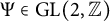
 $$ \begin{align} (\aleph\circ \Xi)\cdot f=\aleph\cdot (\Xi\cdot f). \end{align} $$
To prove (11), let
 $\aleph x=\Psi x+b$
for
$\aleph x=\Psi x+b$
for
 $\Psi \in \mathrm {GL}(2,\mathbb Z)$
and
$\Psi \in \mathrm {GL}(2,\mathbb Z)$
and
 $b\in \mathbb Z^2$
. Hence,
$b\in \mathbb Z^2$
. Hence,
 $(\aleph \circ \Xi )(x)=\Psi \Phi x+\Psi a+b$
and
$(\aleph \circ \Xi )(x)=\Psi \Phi x+\Psi a+b$
and
 $$ \begin{align*} \Big((\aleph\circ \Xi)\cdot f\Big)(x)&=e^{\langle \Psi a+b,x\rangle} f(\Phi^T\Psi^Tx)= e^{\langle b,x\rangle}e^{\langle a,\Psi^T x\rangle}f(\Phi^T\Psi^Tx) \\ &=e^{\langle b,x\rangle}(\Xi\cdot f)(\Psi^T x)=\Big(\aleph\cdot (\Xi\cdot f)\Big)(x). \end{align*} $$
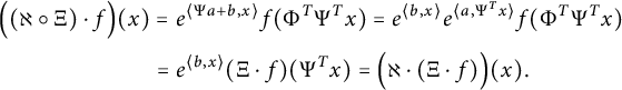
We observe that this action of a
 $\Xi \in \mathcal {G}(\mathbb Z^2)$
satisfies that for a valuation
$\Xi \in \mathcal {G}(\mathbb Z^2)$
satisfies that for a valuation
 $Z:\mathcal {P}(\mathbb Z^2)\to \mathcal {M}(\mathbb R^2)$
, we have
$Z:\mathcal {P}(\mathbb Z^2)\to \mathcal {M}(\mathbb R^2)$
, we have
 $\Xi \cdot Z(P)=Z(\Xi P)$
for
$\Xi \cdot Z(P)=Z(\Xi P)$
for
 $P\in \mathcal {P}(\mathbb Z^2)$
.
$P\in \mathcal {P}(\mathbb Z^2)$
.
Formula (11) readily yields the following property.
Lemma 6 Let
 $P\in \mathcal {P}(\mathbb Z^2)$
, and let
$P\in \mathcal {P}(\mathbb Z^2)$
, and let
 $H\subset \mathcal {G}(\mathbb Z^2)$
be the subgroup of all
$H\subset \mathcal {G}(\mathbb Z^2)$
be the subgroup of all
 $\Xi \in \mathcal {G}(\mathbb Z^2)$
such that
$\Xi \in \mathcal {G}(\mathbb Z^2)$
such that
 $\Xi P=P$
.
$\Xi P=P$
.
For a set
 $\{\Xi _i\}_{i\in I}$
of group generators of H, if
$\{\Xi _i\}_{i\in I}$
of group generators of H, if
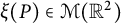 $\xi (P)\in \mathcal {M}(\mathbb R^2)$
satisfies
$\xi (P)\in \mathcal {M}(\mathbb R^2)$
satisfies
 $\Xi _i\cdot \xi (P)=\xi (P)$
for
$\Xi _i\cdot \xi (P)=\xi (P)$
for
 $i\in I$
, then setting
$i\in I$
, then setting
 $\xi (\aleph P)\in \mathcal {M}(\mathbb R^2)$
via
$\xi (\aleph P)\in \mathcal {M}(\mathbb R^2)$
via
 $\xi (\aleph P)=\aleph \cdot \xi (P)$
for any
$\xi (\aleph P)=\aleph \cdot \xi (P)$
for any
 $\aleph \in \mathcal {G}(\mathbb Z^2)$
is well-defined, and satisfies
$\aleph \in \mathcal {G}(\mathbb Z^2)$
is well-defined, and satisfies
 $$ \begin{align*}\xi\Big(\Gamma(\aleph P)\Big)=\Gamma\cdot \xi(\aleph P) \text{for any } \Gamma\in \mathcal{G}(\mathbb Z^2). \end{align*} $$
For a
 $P\in \mathcal {P}(\mathbb Z^2)$
, Lemma 7 is used to determine the subgroup
$P\in \mathcal {P}(\mathbb Z^2)$
, Lemma 7 is used to determine the subgroup
 $\mathcal {G}(\mathbb Z^2)$
fixing P. For a
$\mathcal {G}(\mathbb Z^2)$
fixing P. For a
 $\Xi \in \mathcal {G}(\mathbb Z^2)$
with
$\Xi \in \mathcal {G}(\mathbb Z^2)$
with
 $\Xi x=\Phi x+a$
,
$\Xi x=\Phi x+a$
,
 $\Phi \in \mathrm {GL}(2,\mathbb Z)$
, and
$\Phi \in \mathrm {GL}(2,\mathbb Z)$
, and
 $a\in \mathbb Z^2$
, we set
$a\in \mathbb Z^2$
, we set
 $\det \Xi =\det \Phi $
. Since
$\det \Xi =\det \Phi $
. Since
 $\det : \mathcal {G}(\mathbb Z^2)\to \{-1,1\}$
is a group homomorphism, and a vertex of P is mapped to a vertex of the image by an affine transform (where endpoints of segments are understood as vertices), we deduce the following. We call a
$\det : \mathcal {G}(\mathbb Z^2)\to \{-1,1\}$
is a group homomorphism, and a vertex of P is mapped to a vertex of the image by an affine transform (where endpoints of segments are understood as vertices), we deduce the following. We call a
 $\Xi \in \mathcal {G}(\mathbb Z^2)$
orientation preserving if
$\Xi \in \mathcal {G}(\mathbb Z^2)$
orientation preserving if
 $\det \Xi =1$
.
$\det \Xi =1$
.
Lemma 7 Let
 $P\in \mathcal {P}(\mathbb Z^2)$
such that o is a vertex, let
$P\in \mathcal {P}(\mathbb Z^2)$
such that o is a vertex, let
 $H\subset \mathcal {G}(\mathbb Z^2)$
be the subgroup of all
$H\subset \mathcal {G}(\mathbb Z^2)$
be the subgroup of all
 $\Xi \in \mathcal {G}(\mathbb Z^2)$
such that
$\Xi \in \mathcal {G}(\mathbb Z^2)$
such that
 $\Xi P=P$
, and let
$\Xi P=P$
, and let
 $H_+\subset H$
be the subgroup of orientation preserving transformations in H.
$H_+\subset H$
be the subgroup of orientation preserving transformations in H.
-
(i)
$\Xi (v)$
is a vertex of P for any vertex v of P and
$\Xi \in H$
; -
(ii) if there exists
$\widetilde {\Xi }\in \mathcal {G}(\mathbb Z^2)$
with
$\widetilde {\Xi } P=P$
and
$\det \widetilde {\Xi }=-1$
, then
$H_+$
and
$\widetilde {\Xi }$
generate H; -
(iii) if P is a polygon and
$\Xi (o)=\Xi '(o)$
for
$\Xi ,\Xi '\in H_+$
, then
$\Xi =\Xi '$
.


For a subgroup
 $G\subset \mathcal {G}(\mathbb Z^2)$
, we say that a valuation
$G\subset \mathcal {G}(\mathbb Z^2)$
, we say that a valuation
 $Z:\mathcal {P}(\mathbb Z^2)\to \mathcal {M}(\mathbb R^2)$
is G covariant if
$Z:\mathcal {P}(\mathbb Z^2)\to \mathcal {M}(\mathbb R^2)$
is G covariant if
 $$ \begin{align} Z(\Xi P)(x)=\Big(\Xi\cdot Z(P)\Big)(x)\text{for any } \Xi\in G, P\in \mathcal{P}(\mathbb Z^2) \text{ and } x\in\mathbb R^2. \end{align} $$
In particular, Z is
 $\mathcal {G}(\mathbb Z^2)$
covariant if and only if Z is translatively exponential (cf. (4)) and
$\mathcal {G}(\mathbb Z^2)$
covariant if and only if Z is translatively exponential (cf. (4)) and
 $\mathrm {GL}(2,\mathbb Z)$
covariant (cf. (5)).
$\mathrm {GL}(2,\mathbb Z)$
covariant (cf. (5)).
Next, we show that a
 $\mathcal {G}(\mathbb Z^2)$
covariant valuation
$\mathcal {G}(\mathbb Z^2)$
covariant valuation
 $Z:\mathcal {P}(\mathbb Z^2)\to \mathcal {M}(\mathbb R^2)$
is determined by its value at
$Z:\mathcal {P}(\mathbb Z^2)\to \mathcal {M}(\mathbb R^2)$
is determined by its value at
 $\{o\}$
,
$\{o\}$
,
 $[o,e_1]$
, and T. We note that McMullen [Reference McMullen16] proved the Inclusion–Exclusion principle for any valuation
$[o,e_1]$
, and T. We note that McMullen [Reference McMullen16] proved the Inclusion–Exclusion principle for any valuation
 $Z:\mathcal {P}(\mathbb Z^m)\to \mathcal {A}$
where
$Z:\mathcal {P}(\mathbb Z^m)\to \mathcal {A}$
where
 $\mathcal {A}$
is a cancellative semigroup; namely, if P is a d-dimensional lattice polytope,
$\mathcal {A}$
is a cancellative semigroup; namely, if P is a d-dimensional lattice polytope,
 $1\leq d\leq m$
, and
$1\leq d\leq m$
, and
 $P=Q_1\cup \ldots \cup Q_k$
for d-dimensional lattice polytopes
$P=Q_1\cup \ldots \cup Q_k$
for d-dimensional lattice polytopes
 $Q_1,\ldots , Q_k$
,
$Q_1,\ldots , Q_k$
,
 $k\geq 3$
, such that the non-empty intersection of any subfamily of
$k\geq 3$
, such that the non-empty intersection of any subfamily of
 $Q_1,\ldots , Q_k$
is a lattice polytope, then
$Q_1,\ldots , Q_k$
is a lattice polytope, then
 $$ \begin{align} Z(P)=\sum_{i=1}^k\sum_{1\leq j_1<\cdots<j_i\leq k}(-1)^{i-1}Z(Q_{j_1}\cap\cdots Q_{j_i}) \end{align} $$
where we set
 $Z(\emptyset )=0$
.
$Z(\emptyset )=0$
.
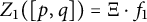
We say that a lattice segment
 $[p,q]$
for
$[p,q]$
for
 $p,q\in \mathbb Z^2$
is a primitive lattice segment if the only lattice points it contains are its endpoints, and a lattice triangle is an empty triangle if the only lattice points it contains are its vertices.
$p,q\in \mathbb Z^2$
is a primitive lattice segment if the only lattice points it contains are its endpoints, and a lattice triangle is an empty triangle if the only lattice points it contains are its vertices.
Proposition 8 For any
 $\mathcal {G}(\mathbb Z^2)$
covariant valuations
$\mathcal {G}(\mathbb Z^2)$
covariant valuations
 $Z,Z':\mathcal {P}(\mathbb Z^2)\to \mathcal {M}(\mathbb R^2)$
,
$Z,Z':\mathcal {P}(\mathbb Z^2)\to \mathcal {M}(\mathbb R^2)$
,
-
(i) if
$Z(\{o\})=Z'(\{o\})$
and
$Z([o,e_1])=Z'([o,e_1])$
, then
$Z-Z'$
is a simple
$\mathcal {G}(\mathbb Z^2)$
covariant valuation; -
(ii) if
$Z(\{o\})=Z'(\{o\})$
,
$Z([o,e_1])=Z'([o,e_1])$
and
$Z(T)=Z'(T)$
, then
$Z=Z'$
.


Proof Let
 $Z(\{o\})=Z'(\{o\})$
and
$Z(\{o\})=Z'(\{o\})$
and
 $Z([o,e_1])=Z'([o,e_1])$
. For any
$Z([o,e_1])=Z'([o,e_1])$
. For any
 $p\in \mathbb Z^2$
, (4) yields that
$p\in \mathbb Z^2$
, (4) yields that
 $$ \begin{align*}Z(\{p\})(x)=e^{\langle x,p\rangle}Z(\{o\})(x)=e^{\langle x,p\rangle}Z'(\{o\})(x)=Z'(\{p\})(x). \end{align*} $$
For a primitive lattice segment
 $[p,q]$
,
$[p,q]$
,
 $p\neq q\in \mathbb Z^2$
, there exists
$p\neq q\in \mathbb Z^2$
, there exists
 $\Phi \in \mathrm {SL}(2,\mathbb Z)$
such that
$\Phi \in \mathrm {SL}(2,\mathbb Z)$
such that
 $[p,q]=p+\Phi [o,e_1]$
; therefore,
$[p,q]=p+\Phi [o,e_1]$
; therefore,
 $Z([p,q])=Z'([p,q])$
by (4) and (5). Now a lattice segment s containing
$Z([p,q])=Z'([p,q])$
by (4) and (5). Now a lattice segment s containing
 $k\geq 3$
lattice points can be subdivided into
$k\geq 3$
lattice points can be subdivided into
 $k-1$
primitive lattice segments, and hence the Inclusion–Exclusion principle (13), together with the just established property that Z and
$k-1$
primitive lattice segments, and hence the Inclusion–Exclusion principle (13), together with the just established property that Z and
 $Z'$
agree on lattice points and primitive segments, yields that
$Z'$
agree on lattice points and primitive segments, yields that
 $Z(s)=Z'(s)$
. In turn, we deduce (i).
$Z(s)=Z'(s)$
. In turn, we deduce (i).
Let us assume that in addition,
 $Z(T)=Z'(T)$
. For an empty lattice triangle
$Z(T)=Z'(T)$
. For an empty lattice triangle
 ${T=[v_1,v_2,v_3]}$
, the vectors
${T=[v_1,v_2,v_3]}$
, the vectors
 $v_2-v_1$
and
$v_2-v_1$
and
 $v_3-v_1$
form a basis of
$v_3-v_1$
form a basis of
 $\mathbb Z^2$
; therefore, there exists a
$\mathbb Z^2$
; therefore, there exists a
 $\Phi \in \mathrm {SL}(2,\mathbb Z)$
such that
$\Phi \in \mathrm {SL}(2,\mathbb Z)$
such that
 $T=v_1+\Phi T$
, which in turn yields that
$T=v_1+\Phi T$
, which in turn yields that
 $Z(T)=Z'(T)$
by (4) and (5). Finally, a two-dimensional lattice polygon P can be written as
$Z(T)=Z'(T)$
by (4) and (5). Finally, a two-dimensional lattice polygon P can be written as
 $P=T_1\cup \cdots \cup T_k$
for empty triangles
$P=T_1\cup \cdots \cup T_k$
for empty triangles
 $T_1,\ldots ,T_k$
such that
$T_1,\ldots ,T_k$
such that
 $T_i\cap T_j$
is either empty, or a common vertex, or a common side. Thus the Inclusion–Exclusion principle (13) together with the property that Z and
$T_i\cap T_j$
is either empty, or a common vertex, or a common side. Thus the Inclusion–Exclusion principle (13) together with the property that Z and
 $Z'$
agree on lattice points, lattice segments, and empty triangles yields that
$Z'$
agree on lattice points, lattice segments, and empty triangles yields that
 $Z(P)=Z'(P)$
.
$Z(P)=Z'(P)$
.
It follows from Proposition 8 that in order to characterize a translatively exponential and
 $\mathrm {GL}(2,\mathbb Z)$
covariant (or equivalently,
$\mathrm {GL}(2,\mathbb Z)$
covariant (or equivalently,
 $\mathcal {G}(\mathbb Z^2)$
covariant) valuation Z on lattice polygons, all we need to characterize are
$\mathcal {G}(\mathbb Z^2)$
covariant) valuation Z on lattice polygons, all we need to characterize are
 $$ \begin{align} Z(\{o\})=f_0\text{ and } Z([o,e_1])=f_1\text{ and } Z(T)=f_2. \end{align} $$
Let us establish some algebraic properties of
 $f_0$
and
$f_0$
and
 $f_1$
in (14). According to Trott [Reference Trott17],
$f_1$
in (14). According to Trott [Reference Trott17],
 $\mathrm {GL}(2,\mathbb Z)$
as a group is generated by
$\mathrm {GL}(2,\mathbb Z)$
as a group is generated by
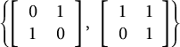 $\left \{ \left [ \begin {array}{cc} 0&1\\ 1&0 \end {array}\right ],\text { } \left [ \begin {array}{cc} 1&1\\ 0&1 \end {array}\right ] \right \} $
, but we do not use this result directly.
$\left \{ \left [ \begin {array}{cc} 0&1\\ 1&0 \end {array}\right ],\text { } \left [ \begin {array}{cc} 1&1\\ 0&1 \end {array}\right ] \right \} $
, but we do not use this result directly.
Lemma 9 Let
 $Z:\mathcal {P}(\mathbb Z^2)\to \mathcal {M}(\mathbb R^2)$
be a
$Z:\mathcal {P}(\mathbb Z^2)\to \mathcal {M}(\mathbb R^2)$
be a
 $\mathcal {G}(\mathbb Z^2)$
covariant valuation. Then
$\mathcal {G}(\mathbb Z^2)$
covariant valuation. Then
 ${Z(\{o\})=f_0}$
and
${Z(\{o\})=f_0}$
and
 $Z([o,e_1])=f_1$
satisfy the following properties:
$Z([o,e_1])=f_1$
satisfy the following properties:
 $$ \begin{align} f_0(\Phi x)&=f_0(x) \text{for any } \Phi\in \mathrm{GL}(2,\mathbb Z) \text{ and } x\in \mathbb R^2; \end{align} $$
 $$ \begin{align} f_1(-x_1,-x_2)&= e^{-x_1}f_1(x_1,x_2)\text{ \ for } (x_1,x_2)\in\mathbb R^2; \end{align} $$
 $$ \begin{align} f_1(x_1,x_2)&= f_1(x_1,x_1+x_2)\text{ \ for} (x_1,x_2)\in\mathbb R^2; \end{align} $$
 $$ \begin{align} f_1(x_1,x_2)&= f_1(x_1,-x_2)\text{ \ for} (x_1,x_2)\in\mathbb R^2. \end{align} $$
Proof Formula (15) follows from (5). The property (16) follows from (4) and the relation
 $\left [ \begin {array}{cc} -1&0\\ 0&-1 \end {array}\right ][o,e_1]=[o,e_1]-e_1$
. Next (17) says that
$\left [ \begin {array}{cc} -1&0\\ 0&-1 \end {array}\right ][o,e_1]=[o,e_1]-e_1$
. Next (17) says that
 $Z([o,e_1])$
is covariant under
$Z([o,e_1])$
is covariant under
 $\left [ \begin {array}{cc} 1&1\\ 0&1 \end {array}\right ]$
, and (18) is the consequence of the fact that
$\left [ \begin {array}{cc} 1&1\\ 0&1 \end {array}\right ]$
, and (18) is the consequence of the fact that
 $Z([o,e_1])$
also is covariant under
$Z([o,e_1])$
also is covariant under
 $\left [ \begin {array}{cc} 1&0\\ 0&-1 \end {array}\right ]$
.
$\left [ \begin {array}{cc} 1&0\\ 0&-1 \end {array}\right ]$
.
3 Some examples of
$\mathcal {G}(\mathbb Z^2)$
covariant valuations on lattice polygons

In this section, we construct two fundamental examples of
 $\mathcal {G}(\mathbb Z^2)$
covariant valuations on
$\mathcal {G}(\mathbb Z^2)$
covariant valuations on
 $\mathcal {P}(\mathbb Z^2)$
. The first is the “positive Laplace transform” that is the basic example of simple valuations satisfying (4) and (5), and the second in Propositions 11 extends a “would be” valuation defined on lattice points and lattice segments.
$\mathcal {P}(\mathbb Z^2)$
. The first is the “positive Laplace transform” that is the basic example of simple valuations satisfying (4) and (5), and the second in Propositions 11 extends a “would be” valuation defined on lattice points and lattice segments.
Example 10 (Positive Laplace transform)
For any lattice polygon P, we define
 $$ \begin{align} \mathcal{L}_+(P)(x)=\int_Pe^{\langle x,y\rangle}\,dy, \end{align} $$
thus
 $\mathcal {L}_+$
is a
$\mathcal {L}_+$
is a
 $\mathcal {G}(\mathbb Z^2)$
covariant simple valuation.
$\mathcal {G}(\mathbb Z^2)$
covariant simple valuation.
We note that (19) yields that
 $$ \begin{align} \mathcal{L}_+(T)(x_1,x_2)=\frac{x_1e^{x_2}-x_2 e^{x_1}+x_2-x_1}{x_1x_2(x_2-x_1)}; \end{align} $$
or in other words, we have
 $$ \begin{align} \mathcal{L}_+(T)(x_1,x_1+x_2)=\frac1{x_1+x_2}\left(e^{x_1}\cdot \frac{e^{x_2}-1}{x_2}- \frac{e^{x_1}-1}{x_1}\right). \end{align} $$
Proposition 11 For
 $f_0,f_1\in \mathcal {M}(\mathbb R^2)$
satisfying (15)–(18), there exists a
$f_0,f_1\in \mathcal {M}(\mathbb R^2)$
satisfying (15)–(18), there exists a
 $\mathcal {G}(\mathbb Z^2)$
covariant valuation
$\mathcal {G}(\mathbb Z^2)$
covariant valuation
 $Z_1:\mathcal {P}(\mathbb Z^2)\to \mathcal {M}(\mathbb R^2)$
satisfying
$Z_1:\mathcal {P}(\mathbb Z^2)\to \mathcal {M}(\mathbb R^2)$
satisfying
 $Z_1(\{o\})=f_0$
and
$Z_1(\{o\})=f_0$
and
 $Z_1([o,e_1])=f_1$
and
$Z_1([o,e_1])=f_1$
and
 $$ \begin{align*}Z_1(T)(x_1,x_2)={\frac12}\,f_1(x_1,x_2)+{\frac12}\,f_1(x_2,-x_1) +{\frac{e^{x_1}}2}\,f_1(-x_1+x_2,-x_1). \end{align*} $$
Proof For points, we define
 $$ \begin{align} Z_1(\{z\})(x)=e^{\langle x,z\rangle}f_0(x) \text{ \ for } z\in\mathbb Z^2 \text{ and } x\in \mathbb R^2. \end{align} $$
As
 $\mathrm {GL}(2,\mathbb Z)\subset \mathcal {G}(\mathbb Z^2)$
is the stabilizer subgroup of
$\mathrm {GL}(2,\mathbb Z)\subset \mathcal {G}(\mathbb Z^2)$
is the stabilizer subgroup of
 $\{o\}$
, (15) and Lemma 6 yield that
$\{o\}$
, (15) and Lemma 6 yield that
 $Z_1$
as defined in (22) is well-defined and is
$Z_1$
as defined in (22) is well-defined and is
 $\mathcal {G}(\mathbb Z^2)$
covariant on lattice points.
$\mathcal {G}(\mathbb Z^2)$
covariant on lattice points.
Turning to segments, we write H to denote the stabilizer subgroup of
 $[o,e_1]$
in
$[o,e_1]$
in
 $\mathcal {G}(\mathbb Z^2)$
,
$\mathcal {G}(\mathbb Z^2)$
,
 $H_+\subset H$
to denote the orientation preserving stabilizers, and
$H_+\subset H$
to denote the orientation preserving stabilizers, and
 $H_0\subset \mathrm {SL}(2,\mathbb Z)$
to denote the subgroup of all
$H_0\subset \mathrm {SL}(2,\mathbb Z)$
to denote the subgroup of all
 $\Phi \in \mathrm {SL}(2,\mathbb Z)$
with
$\Phi \in \mathrm {SL}(2,\mathbb Z)$
with
 $\Phi e_1=e_1$
. Now
$\Phi e_1=e_1$
. Now
 $H_0$
consists of the matrices of the form
$H_0$
consists of the matrices of the form
 $\left [ \begin {array}{cc} 1&a\\ 0&1 \end {array}\right ]$
for an
$\left [ \begin {array}{cc} 1&a\\ 0&1 \end {array}\right ]$
for an
 $a\in \mathbb Z$
, and hence it is generated by
$a\in \mathbb Z$
, and hence it is generated by
 $\Phi _0=\left [ \begin {array}{cc} 1&1\\ 0&1 \end {array}\right ]$
. Since
$\Phi _0=\left [ \begin {array}{cc} 1&1\\ 0&1 \end {array}\right ]$
. Since
 $\Xi _1[o,e_1]=[o,e_1]$
for
$\Xi _1[o,e_1]=[o,e_1]$
for
 $\Xi _1x=-x+e_1\in H_+\backslash H_0$
, and
$\Xi _1x=-x+e_1\in H_+\backslash H_0$
, and
 $H_0\subset H_+$
is a subgroup of index
$H_0\subset H_+$
is a subgroup of index
 $2$
by Lemma 7 (i), we deduce that
$2$
by Lemma 7 (i), we deduce that
 $H_+$
is generated by
$H_+$
is generated by
 $\Phi _0$
and
$\Phi _0$
and
 $\Xi _1$
. It follows from Lemma 7 (ii) that H is generated by
$\Xi _1$
. It follows from Lemma 7 (ii) that H is generated by
 $\Phi _0$
,
$\Phi _0$
,
 $\Xi _1$
and
$\Xi _1$
and
 $\Phi _{-}=\left [ \begin {array}{cc} 1&0\\ 0&-1 \end {array}\right ]$
.
$\Phi _{-}=\left [ \begin {array}{cc} 1&0\\ 0&-1 \end {array}\right ]$
.
For any primitive lattice segment
 $[p,q]$
there exists
$[p,q]$
there exists
 $\Xi \in \mathcal {G}(\mathbb Z^2)$
such that
$\Xi \in \mathcal {G}(\mathbb Z^2)$
such that
 $\Xi [o,e_1]=[p,q]$
; namely, take
$\Xi [o,e_1]=[p,q]$
; namely, take
 $\Xi x=\Phi x+p$
where
$\Xi x=\Phi x+p$
where
 $q-p=\Phi e_1$
for
$q-p=\Phi e_1$
for
 $\Phi \in \mathrm {SL}(2,\mathbb Z)$
. Since H is generated by
$\Phi \in \mathrm {SL}(2,\mathbb Z)$
. Since H is generated by
 $\Phi _0$
,
$\Phi _0$
,
 $\Xi _1$
, and
$\Xi _1$
, and
 $\Phi _{-}$
where the condition (18) on
$\Phi _{-}$
where the condition (18) on
 $f_1$
corresponds to the
$f_1$
corresponds to the
 $\Phi _{-}$
invariance of
$\Phi _{-}$
invariance of
 $[o,e_1]$
, it follows from Lemma 6 that if
$[o,e_1]$
, it follows from Lemma 6 that if
 $[p,q]$
is a primitive lattice segment, then we may define
$[p,q]$
is a primitive lattice segment, then we may define
 $$ \begin{align} Z_1([p,q])=\Xi\cdot f_1 \end{align} $$
for any
 $\Xi \in \mathcal {G}(\mathbb Z^2)$
with
$\Xi \in \mathcal {G}(\mathbb Z^2)$
with
 $\Xi [o,e_1]=[p,q]$
. Lemma 6 also yields that
$\Xi [o,e_1]=[p,q]$
. Lemma 6 also yields that
 $Z_1$
is
$Z_1$
is
 $\mathcal {G}(\mathbb Z^2)$
covariant on lattice segments.
$\mathcal {G}(\mathbb Z^2)$
covariant on lattice segments.
Now a general lattice segment
 $[a,b]$
for
$[a,b]$
for
 $a\neq b$
,
$a\neq b$
,
 $a,b\in \mathbb Z^2$
is divided into primitive lattice segments by the lattice points contained in
$a,b\in \mathbb Z^2$
is divided into primitive lattice segments by the lattice points contained in
 $[a,b]$
different from
$[a,b]$
different from
 $a,b$
, and hence, using the abbreviation “pls” for primitive lattice segments, we define
$a,b$
, and hence, using the abbreviation “pls” for primitive lattice segments, we define
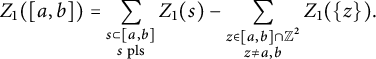 $$ \begin{align} Z_1([a,b])=\sum_{\substack{s\subset[a,b]\\ s\;\mathrm{pls}}}Z_1(s)-\sum_{\substack{z\in [a,b]\cap \mathbb Z^2\\ z\neq a,b}}Z_1(\{z\}). \end{align} $$
Since
 $Z_1$
is translatively exponential and
$Z_1$
is translatively exponential and
 $\mathrm {GL}(\mathbb Z^2)$
covariant on points and primitive lattice segments,
$\mathrm {GL}(\mathbb Z^2)$
covariant on points and primitive lattice segments,
 $Z_1$
is
$Z_1$
is
 $\mathcal {G}(\mathbb Z^2)$
covariant on lattice segments and lattice points.
$\mathcal {G}(\mathbb Z^2)$
covariant on lattice segments and lattice points.
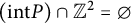
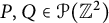
In addition, if P is a lattice polygon, then we define
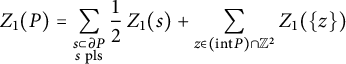 $$ \begin{align} Z_1(P)=\sum_{\substack{s\subset\partial P\\ s\;\mathrm{pls}}} {\frac12\,}Z_1(s)+\sum_{z\in (\mathrm{int} P)\cap \mathbb Z^2}Z_1(\{z\}) \end{align} $$
where the second sum is zero if
 $(\mathrm {int} P)\cap \mathbb Z^2=\emptyset $
.
$(\mathrm {int} P)\cap \mathbb Z^2=\emptyset $
.
 $Z_1$
is readily
$Z_1$
is readily
 $\mathcal {G}(\mathbb Z^2)$
covariant also on polygons. In addition, the (primitive) edges of T are
$\mathcal {G}(\mathbb Z^2)$
covariant also on polygons. In addition, the (primitive) edges of T are
 $[o,e_1]$
,
$[o,e_1]$
,
 $\Phi _1[o,e_1]$
, and
$\Phi _1[o,e_1]$
, and
 $e_1+\Phi _2[o,e_1]$
for
$e_1+\Phi _2[o,e_1]$
for
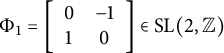 $\Phi _1=\left [ \begin {array}{cc} 0&-1\\ 1&0 \end {array}\right ]\in \mathrm {SL}(2,\mathbb Z)$
and
$\Phi _1=\left [ \begin {array}{cc} 0&-1\\ 1&0 \end {array}\right ]\in \mathrm {SL}(2,\mathbb Z)$
and
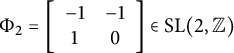 $\Phi _2=\left [ \begin {array}{cc} -1&-1\\ 1&0 \end {array}\right ]\in \mathrm {SL}(2,\mathbb Z)$
, thus (23) and (25) yield
$\Phi _2=\left [ \begin {array}{cc} -1&-1\\ 1&0 \end {array}\right ]\in \mathrm {SL}(2,\mathbb Z)$
, thus (23) and (25) yield
 $$ \begin{align*}Z_1(T)(x,y)={\frac12}\,f_1(x,y)+{\frac12}\,f_1(y,-x) +{\frac{e^{x}}2}\,f_1(-x+y,-x). \end{align*} $$
Therefore, all we have to prove is that the function
 $Z_1$
on
$Z_1$
on
 $\mathcal {P}(\mathbb Z^2)$
defined by (22)–(25) is a valuation; namely, if
$\mathcal {P}(\mathbb Z^2)$
defined by (22)–(25) is a valuation; namely, if
 $P\cup Q$
is convex for
$P\cup Q$
is convex for
 $P,Q\in \mathcal {P}(\mathbb Z^2)$
, then
$P,Q\in \mathcal {P}(\mathbb Z^2)$
, then
 $$ \begin{align} Z_1(P)+Z_1(Q)=Z_1(P\cap Q)+Z_1(P\cup Q). \end{align} $$
If
 $P\subset Q$
or
$P\subset Q$
or
 $Q\subset P$
, then (26) readily holds. Therefore, besides that
$Q\subset P$
, then (26) readily holds. Therefore, besides that
 $P\cup Q$
are convex, we assume that either P and Q are lattice segments not containing each other, or P and Q are lattice polygons not containing each other.
$P\cup Q$
are convex, we assume that either P and Q are lattice segments not containing each other, or P and Q are lattice polygons not containing each other.
Case 1
 $\mathrm {dim}(P\cap Q)<\mathrm {dim}\,P=\mathrm {dim}\,Q$
In other words, either P and Q are collinear lattice segments whose intersection is a common endpoint, or P and Q are lattice polygons whose intersection is a common side, and in addition,
$\mathrm {dim}(P\cap Q)<\mathrm {dim}\,P=\mathrm {dim}\,Q$
In other words, either P and Q are collinear lattice segments whose intersection is a common endpoint, or P and Q are lattice polygons whose intersection is a common side, and in addition,
 $P\cup Q$
is convex. In the first case (24), and in the second case (24) and (25) directly yield (26).
$P\cup Q$
is convex. In the first case (24), and in the second case (24) and (25) directly yield (26).
Case 2
 $\mathrm {dim}(P\cap Q)=\mathrm {dim}\,P=\mathrm {dim}\,Q\geq 1$
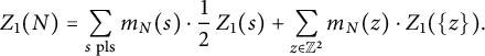
Let us introduce a notion of multiplicity of a primitive lattice segment s and a
$\mathrm {dim}(P\cap Q)=\mathrm {dim}\,P=\mathrm {dim}\,Q\geq 1$
Let us introduce a notion of multiplicity of a primitive lattice segment s and a
 $z\in \mathbb Z^2$
with respect to a general lattice segment
$z\in \mathbb Z^2$
with respect to a general lattice segment
 $[a,b]$
for
$[a,b]$
for
 $a\neq b$
,
$a\neq b$
,
 $a,b\in \mathbb Z^2$
and a lattice polygon N where we set
$a,b\in \mathbb Z^2$
and a lattice polygon N where we set
 $(a,b)=[a,b]\backslash \{a,b\}$
:
$(a,b)=[a,b]\backslash \{a,b\}$
:
 $$ \begin{align*} m_{[a,b]}(s)&=1\text{ if }s\subset[a,b], \ \text{and } m_{[a,b]}(s)=0\text{ otherwise; }\\
m_{[a,b]}(z)&=1\text{ if }z\in(a,b), \ \text{and } m_{[a,b]}(z)=0\text{ otherwise; }\\
m_{N}(s)&=1\text{ if }s\subset\partial N, \ \text{and } m_{N}(s)=0\text{ otherwise; }\\m_{N}(z)&=1\text{ if }z\in\mathrm{int}\,N, \ \text{and } m_{N}(z)=0\text{ otherwise. } \end{align*} $$
$$ \begin{align*} m_{[a,b]}(s)&=1\text{ if }s\subset[a,b], \ \text{and } m_{[a,b]}(s)=0\text{ otherwise; }\\
m_{[a,b]}(z)&=1\text{ if }z\in(a,b), \ \text{and } m_{[a,b]}(z)=0\text{ otherwise; }\\
m_{N}(s)&=1\text{ if }s\subset\partial N, \ \text{and } m_{N}(s)=0\text{ otherwise; }\\m_{N}(z)&=1\text{ if }z\in\mathrm{int}\,N, \ \text{and } m_{N}(z)=0\text{ otherwise. } \end{align*} $$
In particular,
 $$ \begin{align} Z_1([a,b])&=\sum_{s\;\mathrm{pls}}m_{[a,b]}(s)\cdot Z_1(s)-\sum_{z\in\mathbb Z^2}m_{[a,b]}(z)\cdot Z_1(\{z\}) \end{align} $$
 $$ \begin{align}Z_1(N)&=\sum_{s\;\mathrm{pls}}m_{N}(s)\cdot {\frac12\,}Z_1(s)+\sum_{z\in\mathbb Z^2}m_{N}(z)\cdot Z_1(\{z\}). \end{align} $$
If
 $P,Q\in \mathcal {P}(\mathbb Z^2)$
satisfy that
$P,Q\in \mathcal {P}(\mathbb Z^2)$
satisfy that
 $P\cup Q$
is convex and
$P\cup Q$
is convex and
 $\mathrm {dim}(P\cap Q)=\mathrm {dim}\,P=\mathrm {dim}\,Q\geq 1$
, and if s is a primitive lattice segment and
$\mathrm {dim}(P\cap Q)=\mathrm {dim}\,P=\mathrm {dim}\,Q\geq 1$
, and if s is a primitive lattice segment and
 $z\in \mathbb Z^2$
, then we claim that
$z\in \mathbb Z^2$
, then we claim that
 $$ \begin{align} m_{P}(s)+m_{Q}(s)&= m_{P\cap Q}(s)+m_{P\cup Q}(s) \end{align} $$
 $$ \begin{align} m_{P}(z)+m_{Q}(z)&= m_{P\cap Q}(z)+m_{P\cup Q}(z). \end{align} $$
If
 $\mathrm {dim}(P\cap Q)=\mathrm {dim}\,P=\mathrm {dim}\,Q= 1$
, then
$\mathrm {dim}(P\cap Q)=\mathrm {dim}\,P=\mathrm {dim}\,Q= 1$
, then
 $(\mathrm {relint}\,P)\cup (\mathrm {relint}\,Q)=\mathrm {relint}(P\cup Q)$
(where
$(\mathrm {relint}\,P)\cup (\mathrm {relint}\,Q)=\mathrm {relint}(P\cup Q)$
(where
 $\mathrm {relint}\,P$
is the open segment determined by P), and hence
$\mathrm {relint}\,P$
is the open segment determined by P), and hence
 $z\in (\mathrm {relint}\,P)\cap (\mathrm {relint}\,Q)$
if and only if
$z\in (\mathrm {relint}\,P)\cap (\mathrm {relint}\,Q)$
if and only if
 $z\in \mathrm {relint}\,P$
and
$z\in \mathrm {relint}\,P$
and
 $z\in \mathrm {relint}\,Q$
. Since
$z\in \mathrm {relint}\,Q$
. Since
 $s\subset P\cap Q$
for a primitive lattice segment s if and only if
$s\subset P\cap Q$
for a primitive lattice segment s if and only if
 $s\subset P$
and
$s\subset P$
and
 $s\subset Q$
, we conclude (29) and (30).
$s\subset Q$
, we conclude (29) and (30).
Let
 $\mathrm {dim}(P\cap Q)=\mathrm {dim}\,P=\mathrm {dim}\,Q= 2$
, and hence
$\mathrm {dim}(P\cap Q)=\mathrm {dim}\,P=\mathrm {dim}\,Q= 2$
, and hence
 $$ \begin{align} \text{no line separates } P \text{ and } Q. \end{align} $$
For (30), if
 $x\in \mathrm {int}(P\cup Q)$
and
$x\in \mathrm {int}(P\cup Q)$
and
 $x\in \partial P$
, then there exists a supporting line
$x\in \partial P$
, then there exists a supporting line
 $\ell $
to P at x. Now any small semicircle centered at x and separated from P by
$\ell $
to P at x. Now any small semicircle centered at x and separated from P by
 $\ell $
is contained in Q, and (31) yields that
$\ell $
is contained in Q, and (31) yields that
 $x\in \mathrm {int}\,Q$
. The similar argument if
$x\in \mathrm {int}\,Q$
. The similar argument if
 $x\in \mathrm {int}(P\cup Q)$
and
$x\in \mathrm {int}(P\cup Q)$
and
 $x\in \partial Q$
shows that
$x\in \partial Q$
shows that
 $(\mathrm {int}\,P)\cup (\mathrm {int}\,Q)=\mathrm {int}(P\cup Q)$
, which in turn implies (30). For (29), we deduce from the convexity of
$(\mathrm {int}\,P)\cup (\mathrm {int}\,Q)=\mathrm {int}(P\cup Q)$
, which in turn implies (30). For (29), we deduce from the convexity of
 $P\cup Q$
that each vertex of
$P\cup Q$
that each vertex of
 $P\cap Q$
is a vertex of P or Q (see, e.g., McMullen [Reference McMullen16]), and hence the primitive lattice segment s is contained in
$P\cap Q$
is a vertex of P or Q (see, e.g., McMullen [Reference McMullen16]), and hence the primitive lattice segment s is contained in
 $\partial (P\cup Q)$
or
$\partial (P\cup Q)$
or
 $\partial (P\cap Q)$
if and only if s is contained in
$\partial (P\cap Q)$
if and only if s is contained in
 $\partial \,P$
or
$\partial \,P$
or
 $\partial \,Q$
. We deduce from (31) that if
$\partial \,Q$
. We deduce from (31) that if
 $s\subset (\partial \,P)\cap (\partial \,Q)$
, then
$s\subset (\partial \,P)\cap (\partial \,Q)$
, then
 $s\subset \partial (P\cup Q)$
and
$s\subset \partial (P\cup Q)$
and
 $s\subset \partial (P\cap Q)$
; therefore, (29) holds, as well.
$s\subset \partial (P\cap Q)$
; therefore, (29) holds, as well.
Combining (27)–(30) yields (26), and in turn Proposition 11.
Propositions 8 (i) and 11 yield the following.
Corollary 12 For any
 $\mathcal {G}(\mathbb Z^2)$
covariant valuation
$\mathcal {G}(\mathbb Z^2)$
covariant valuation
 $Z:\mathcal {P}(\mathbb Z^2)\to \mathcal {M}(\mathbb R^2)$
, let
$Z:\mathcal {P}(\mathbb Z^2)\to \mathcal {M}(\mathbb R^2)$
, let
 $Z_1$
be the
$Z_1$
be the
 $\mathcal {G}(\mathbb Z^2)$
covariant valuation satisfying
$\mathcal {G}(\mathbb Z^2)$
covariant valuation satisfying
 $Z_1(\{o\})=Z(\{o\})$
and
$Z_1(\{o\})=Z(\{o\})$
and
 $Z_1([o,e_1])=Z([o,e_1])$
constructed in Proposition 11. Then
$Z_1([o,e_1])=Z([o,e_1])$
constructed in Proposition 11. Then
 $Z_2=Z-Z_1$
is a
$Z_2=Z-Z_1$
is a
 $\mathcal {G}(\mathbb Z^2)$
covariant simple valuation.
$\mathcal {G}(\mathbb Z^2)$
covariant simple valuation.
4 Algebraic properties of simple valuations
Having Lemma 9 and Corollary 12 at hand, an algebraic characterization of simple
 $\mathcal {G}(\mathbb Z^2)$
covariant valuations leads to an algebraic characterization of all
$\mathcal {G}(\mathbb Z^2)$
covariant valuations leads to an algebraic characterization of all
 $\mathcal {G}(\mathbb Z^2)$
covariant valuations.
$\mathcal {G}(\mathbb Z^2)$
covariant valuations.
Lemma 13 For any simple
 $\mathcal {G}(\mathbb Z^2)$
covariant valuation
$\mathcal {G}(\mathbb Z^2)$
covariant valuation
 $Z:\mathcal {P}(\mathbb Z^2)\to \mathcal {M}(\mathbb R^2)$
,
$Z:\mathcal {P}(\mathbb Z^2)\to \mathcal {M}(\mathbb R^2)$
,
 $Z(T)=f_2$
satisfies the following properties: For
$Z(T)=f_2$
satisfies the following properties: For
 $x,y\in \mathbb R$
, we have
$x,y\in \mathbb R$
, we have
 $$ \begin{align}\kern-14pt f_2(-x+y,-x)&= e^{-x}f_2(x,y); \end{align} $$
 $$ \begin{align} f_2(x,y)+e^{x+y}f_2(-x,-y)&=f_2(x,x+y)+f_2(x+y,y); \end{align} $$
 $$ \begin{align} f_2(x,y)&= f_2(y,x). \end{align} $$
Proof The
 $\mathcal {G}(\mathbb Z^2)$
covariance yields (32) because
$\mathcal {G}(\mathbb Z^2)$
covariance yields (32) because
 $T-e_1=\left [ \begin {array}{cc} -1&-1\\ 1&0 \end {array}\right ] T$
.
$T-e_1=\left [ \begin {array}{cc} -1&-1\\ 1&0 \end {array}\right ] T$
.
For (33), we observe that each diagonal of the square
 $[0,1]^2$
cuts the square into two empty triangles. In particular,
$[0,1]^2$
cuts the square into two empty triangles. In particular,
 $[0,1]^2$
can be written as
$[0,1]^2$
can be written as
 $T\cup (e_1+e_2-T)$
on the one hand, and the union of the triangles
$T\cup (e_1+e_2-T)$
on the one hand, and the union of the triangles
 $\left [ \begin {array}{cc} 1&1\\ 0&1 \end {array}\right ] T$
and
$\left [ \begin {array}{cc} 1&1\\ 0&1 \end {array}\right ] T$
and
 $\left [ \begin {array}{cc} 1&0\\ 1&1 \end {array}\right ] T$
on the other hand. We conclude (33) from evaluating
$\left [ \begin {array}{cc} 1&0\\ 1&1 \end {array}\right ] T$
on the other hand. We conclude (33) from evaluating
 $Z([0,1]^2)$
in the two ways; and using the simpleness of Z and the
$Z([0,1]^2)$
in the two ways; and using the simpleness of Z and the
 $\mathcal {G}(\mathbb Z^2)$
covariance of Z.
$\mathcal {G}(\mathbb Z^2)$
covariance of Z.
Finally, (34) follows from
 $T=\left [ \begin {array}{cc} 0&1\\ 1&0 \end {array}\right ] T$
and the
$T=\left [ \begin {array}{cc} 0&1\\ 1&0 \end {array}\right ] T$
and the
 $\mathcal {G}(\mathbb Z^2)$
covariance of Z.
$\mathcal {G}(\mathbb Z^2)$
covariance of Z.
Proposition 14 For any
 $f_2\in \mathcal {M}(\mathbb R^2)$
satisfying the properties (32)–(34) in Lemma 13, there exists a unique simple
$f_2\in \mathcal {M}(\mathbb R^2)$
satisfying the properties (32)–(34) in Lemma 13, there exists a unique simple
 $\mathcal {G}(\mathbb Z^2)$
covariant valuation
$\mathcal {G}(\mathbb Z^2)$
covariant valuation
 $Z:\mathcal {P}(\mathbb Z^2)\to \mathcal {M}(\mathbb R^2)$
such that
$Z:\mathcal {P}(\mathbb Z^2)\to \mathcal {M}(\mathbb R^2)$
such that
 $Z(T)=f_2$
.
$Z(T)=f_2$
.
Proof We write H to denote the subgroup of stabilizers of T of
 $\mathcal {G}(\mathbb Z^2)$
, and let
$\mathcal {G}(\mathbb Z^2)$
, and let
 $H_+\subset H$
be the subgroup of orientation preserving transformations.
$H_+\subset H$
be the subgroup of orientation preserving transformations.
In accordance with Lemma 7,
 $H_+$
has three elements corresponding to the vertices of T; namely, the identity,
$H_+$
has three elements corresponding to the vertices of T; namely, the identity,
 $\Xi _+x=\Phi _+x+e_1$
for
$\Xi _+x=\Phi _+x+e_1$
for
 $\Phi _+=\left [ \begin {array}{cc} -1&-1\\ 1&0 \end {array}\right ]$
where
$\Phi _+=\left [ \begin {array}{cc} -1&-1\\ 1&0 \end {array}\right ]$
where
 $\Xi _+T=T$
, and
$\Xi _+T=T$
, and
 $\Xi _+^{-1}x=\Phi _+^{-1}x+e_2$
where
$\Xi _+^{-1}x=\Phi _+^{-1}x+e_2$
where
 $\Phi _+^{-1}=\left [ \begin {array}{cc} 0&1\\ -1&-1 \end {array}\right ]$
. It followsfrom Lemma 7 (ii) that H is generated by
$\Phi _+^{-1}=\left [ \begin {array}{cc} 0&1\\ -1&-1 \end {array}\right ]$
. It followsfrom Lemma 7 (ii) that H is generated by
 $\Xi _+$
and
$\Xi _+$
and
 $\Phi _{-}=\left [ \begin {array}{cc} 0&1\\ 1&0 \end {array}\right ]$
. Since the property (32) of
$\Phi _{-}=\left [ \begin {array}{cc} 0&1\\ 1&0 \end {array}\right ]$
. Since the property (32) of
 $f_2$
corresponds to the
$f_2$
corresponds to the
 $\Xi _+$
invariance of T, and the property (34) of
$\Xi _+$
invariance of T, and the property (34) of
 $f_2$
corresponds to the
$f_2$
corresponds to the
 $\Phi _{-}$
invariance of T, it follows from Lemma 6 that we may define
$\Phi _{-}$
invariance of T, it follows from Lemma 6 that we may define
 $Z_2(N)$
for any empty triangle N by choosing a
$Z_2(N)$
for any empty triangle N by choosing a
 $\Xi \in \mathcal {G}(\mathbb Z^2)$
with
$\Xi \in \mathcal {G}(\mathbb Z^2)$
with
 $N=\Xi T$
and setting
$N=\Xi T$
and setting
 $$ \begin{align} Z_2(N)=\Xi\cdot f_2. \end{align} $$
In addition, the
 $Z_2$
defined as in (35) is
$Z_2$
defined as in (35) is
 $\mathcal {G}(\mathbb Z^2)$
covariant on empty lattice triangles according to Lemma 6.
$\mathcal {G}(\mathbb Z^2)$
covariant on empty lattice triangles according to Lemma 6.
Next we call a parallelogram
 $P\in \mathcal {P}(\mathbb Z^2)$
an empty parallelogram if contains no other lattice points then its vertices. In this case,
$P\in \mathcal {P}(\mathbb Z^2)$
an empty parallelogram if contains no other lattice points then its vertices. In this case,
 $P=\Xi [0,1]^2$
for a
$P=\Xi [0,1]^2$
for a
 $\Xi \in \mathcal {G}(\mathbb Z^2)$
.
$\Xi \in \mathcal {G}(\mathbb Z^2)$
.
For an empty parallelogram
 $P\in \mathcal {P}(\mathbb Z^2)$
, one of the diagonals of P cuts P into the two empty triangles, let them be
$P\in \mathcal {P}(\mathbb Z^2)$
, one of the diagonals of P cuts P into the two empty triangles, let them be
 $T_1$
and
$T_1$
and
 $T_2$
, and let
$T_2$
, and let
 $T_3$
and
$T_3$
and
 $T_4$
be the two empty triangles in P determined by the other diagonal of P. We claim that
$T_4$
be the two empty triangles in P determined by the other diagonal of P. We claim that
 $$ \begin{align} Z_2(T_1)+Z_2(T_2)=Z_2(T_3)+Z_2(T_4). \end{align} $$
Let v be the vertex of
 $T_1$
that is not a vertex of
$T_1$
that is not a vertex of
 $T_2$
, and let
$T_2$
, and let
 $\Xi \in \mathcal {G}(\mathbb Z^2)$
such that
$\Xi \in \mathcal {G}(\mathbb Z^2)$
such that
 $P=\Xi [0,1]^2$
and
$P=\Xi [0,1]^2$
and
 $\Xi o=v$
. For
$\Xi o=v$
. For
 $\widetilde {\Xi }_1=I_2$
and
$\widetilde {\Xi }_1=I_2$
and
 $\widetilde \Xi _2x=-x+e_1+e_2$
, the diagonal
$\widetilde \Xi _2x=-x+e_1+e_2$
, the diagonal
 $[e_1,e_2]$
of
$[e_1,e_2]$
of
 $[0,1]^2$
divides the square into
$[0,1]^2$
divides the square into
 $\widetilde {\Xi }_1T$
and
$\widetilde {\Xi }_1T$
and
 $\widetilde {\Xi }_2T$
, and
$\widetilde {\Xi }_2T$
, and
 $T_i=\Xi \,\widetilde {\Xi }_iT$
for
$T_i=\Xi \,\widetilde {\Xi }_iT$
for
 $i=1,2$
. Possibly after interchanging
$i=1,2$
. Possibly after interchanging
 $T_3$
and
$T_3$
and
 $T_4$
, we may assume that
$T_4$
, we may assume that
 $T_i=\Xi \,\widetilde {\Xi }_iT$
for
$T_i=\Xi \,\widetilde {\Xi }_iT$
for
 $i=3,4$
where
$i=3,4$
where
 $\widetilde {\Xi }_3=\left [ \begin {array}{cc} 1&1\\ 0&1 \end {array}\right ]$
and
$\widetilde {\Xi }_3=\left [ \begin {array}{cc} 1&1\\ 0&1 \end {array}\right ]$
and
 $\widetilde {\Xi }_4=\left [ \begin {array}{cc} 1&0\\ 1&1 \end {array}\right ]$
, and the diagonal
$\widetilde {\Xi }_4=\left [ \begin {array}{cc} 1&0\\ 1&1 \end {array}\right ]$
, and the diagonal
 $[o,e_1+e_2]$
of
$[o,e_1+e_2]$
of
 $[0,1]^2$
divides the square into
$[0,1]^2$
divides the square into
 $\widetilde {\Xi }_3T$
and
$\widetilde {\Xi }_3T$
and
 $\widetilde {\Xi }_4T$
. Since (33) states that
$\widetilde {\Xi }_4T$
. Since (33) states that
 $$ \begin{align*}\widetilde{\Xi}_1\cdot f_2+\widetilde{\Xi}_2\cdot f_2=\widetilde{\Xi}_3\cdot f_2+\widetilde{\Xi}_4\cdot f_2, \end{align*} $$
we conclude (36) from the definition and
 $\mathcal {G}(\mathbb Z^2)$
covariance of
$\mathcal {G}(\mathbb Z^2)$
covariance of
 $Z_2$
for empty triangles.
$Z_2$
for empty triangles.
To define
 $Z_2(Q)$
for a lattice polygon
$Z_2(Q)$
for a lattice polygon
 $Q\in \mathcal {P}(\mathbb Z^2)$
, to any triangulation
$Q\in \mathcal {P}(\mathbb Z^2)$
, to any triangulation
 $\mathcal {T}=\{E_1,\ldots ,E_k\}$
into empty triangles, we assign
$\mathcal {T}=\{E_1,\ldots ,E_k\}$
into empty triangles, we assign
 $$ \begin{align*}\xi(\mathcal{T})=\sum_{i=1}^kZ_2(E_i). \end{align*} $$
We claim that if
 $\mathcal {T}'=\{E^{\prime }_1,\ldots ,E^{\prime }_k\}$
is another triangulation of Q into empty triangles, then
$\mathcal {T}'=\{E^{\prime }_1,\ldots ,E^{\prime }_k\}$
is another triangulation of Q into empty triangles, then
 $$ \begin{align} \xi(\mathcal{T})=\xi(\mathcal{T}'). \end{align} $$
According to Lawson [Reference Lawson11] (see de Loera et al. [Reference de Loera, Rambau and Santos7, Section 3.4.1],), the two triangulations
 $\mathcal {T}$
and
$\mathcal {T}$
and
 $\mathcal {T}'$
can be connected by a series of triangulations
$\mathcal {T}'$
can be connected by a series of triangulations
 $\mathcal {T}_0,\ldots ,\mathcal {T}_m$
of Q into empty triangles such that
$\mathcal {T}_0,\ldots ,\mathcal {T}_m$
of Q into empty triangles such that
 $\mathcal {T}=\mathcal {T}_0$
,
$\mathcal {T}=\mathcal {T}_0$
,
 $\mathcal {T}'=\mathcal {T}_m$
, and
$\mathcal {T}'=\mathcal {T}_m$
, and
 $\mathcal {T}_{i+1}$
is obtained by a diagonal flip from
$\mathcal {T}_{i+1}$
is obtained by a diagonal flip from
 $\mathcal {T}_i$
. Here a diagonal flip means that we find two empty triangles
$\mathcal {T}_i$
. Here a diagonal flip means that we find two empty triangles
 $T_1$
and
$T_1$
and
 $T_2$
in
$T_2$
in
 $\mathcal {T}_i$
whose union is an empty parallelogram P, and hence
$\mathcal {T}_i$
whose union is an empty parallelogram P, and hence
 $T_1\cap T_2$
is a diagonal of P, and we replace
$T_1\cap T_2$
is a diagonal of P, and we replace
 $T_1$
and
$T_1$
and
 $T_2$
by the two empty triangles
$T_2$
by the two empty triangles
 $T_3$
and
$T_3$
and
 $T_4$
obtained by cutting P into two by the other diagonal of P. We deduce from (36) that
$T_4$
obtained by cutting P into two by the other diagonal of P. We deduce from (36) that
 $\xi (\mathcal {T}_{i+1})=\xi (\mathcal {T}_i)$
, yielding (37).
$\xi (\mathcal {T}_{i+1})=\xi (\mathcal {T}_i)$
, yielding (37).
It follows from (37) that for any lattice polygon
 $Q\in \mathcal {P}(\mathbb Z^2)$
, we can define
$Q\in \mathcal {P}(\mathbb Z^2)$
, we can define
 $Z_2(Q)$
by subdividing Q into empty lattice triangles
$Z_2(Q)$
by subdividing Q into empty lattice triangles
 $E_1,\ldots ,E_k$
, and setting
$E_1,\ldots ,E_k$
, and setting
 $$ \begin{align} Z_2(Q)=\sum_{i=1}^kZ_2(E_i). \end{align} $$
If
 $P\in \mathcal {P}(\mathbb Z^2)$
is a point or a segment, then we define
$P\in \mathcal {P}(\mathbb Z^2)$
is a point or a segment, then we define
 $Z_2(P)=0$
. Since
$Z_2(P)=0$
. Since
 $Z_2$
has been known to be
$Z_2$
has been known to be
 $\mathcal {G}(\mathbb Z^2)$
contravariant on empty triangles,
$\mathcal {G}(\mathbb Z^2)$
contravariant on empty triangles,
 $Z_2$
is
$Z_2$
is
 $\mathcal {G}(\mathbb Z^2)$
contravariant on
$\mathcal {G}(\mathbb Z^2)$
contravariant on
 $\mathcal {P}(\mathbb Z^2)$
.
$\mathcal {P}(\mathbb Z^2)$
.
Therefore, all left to prove is that
 $Z_2$
is a simple valuation. To verify this, we only need to check the case when
$Z_2$
is a simple valuation. To verify this, we only need to check the case when
 $P,Q\in \mathcal {P}(\mathbb Z^2)$
are lattice polygons such that
$P,Q\in \mathcal {P}(\mathbb Z^2)$
are lattice polygons such that
 $P\cup Q$
is convex and
$P\cup Q$
is convex and
 $P\cap Q$
is also a lattice polygon. First, we subdivide
$P\cap Q$
is also a lattice polygon. First, we subdivide
 $P\cap Q$
into empty triangles, which triangulation we extend into a triangulation
$P\cap Q$
into empty triangles, which triangulation we extend into a triangulation
 $\mathcal {T}_P$
of P and a triangulation
$\mathcal {T}_P$
of P and a triangulation
 $\mathcal {T}_Q$
of Q into empty triangles. It follows that
$\mathcal {T}_Q$
of Q into empty triangles. It follows that
 $\mathcal {T}_P\cap \mathcal {T}_Q$
is the original triangulation of
$\mathcal {T}_P\cap \mathcal {T}_Q$
is the original triangulation of
 $P\cap Q$
, and
$P\cap Q$
, and
 $\mathcal {T}_P\cup \mathcal {T}_Q$
is a triangulation of
$\mathcal {T}_P\cup \mathcal {T}_Q$
is a triangulation of
 $P\cup Q$
. Therefore, (38) yields that
$P\cup Q$
. Therefore, (38) yields that
 $Z_2(P\cup Q)+Z_2(P\cap Q)=Z_2(P)+Z_2(Q)$
.
$Z_2(P\cup Q)+Z_2(P\cap Q)=Z_2(P)+Z_2(Q)$
.
We note that for any
 $a,b\in \mathbb N$
, the function
$a,b\in \mathbb N$
, the function
 $$ \begin{align} (x,y)\mapsto \frac1{x-y}\left(\frac{e^{y}-1}{y}\cdot x^ay^b-\frac{e^{x}-1}{x}\cdot x^by^a\right) \end{align} $$
is analytic.
Example 15 Since the analytic function (cf. (39))
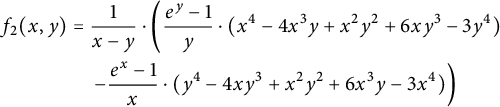 $$ \begin{align*} f_2(x,y) &= \frac1{x-y}\cdot \left(\frac{e^{y}-1}{y}\cdot(x^4-4x^3y+x^2y^2+6xy^3-3y^4)\right.\\ & \quad \left.-\frac{e^{x}-1}{x}\cdot (y^4-4xy^3+x^2y^2+6x^3y-3x^4)\right) \end{align*} $$
satisfies (32)–(34), it follows from Proposition 14 that there exists a
 $\mathcal {G}(\mathbb Z^2)$
covariant simple valuation
$\mathcal {G}(\mathbb Z^2)$
covariant simple valuation
 $Z:\mathcal {P}(\mathbb Z^2)\to \mathcal {M}(\mathbb R^2)$
satisfying
$Z:\mathcal {P}(\mathbb Z^2)\to \mathcal {M}(\mathbb R^2)$
satisfying
 $Z(T)=f_2$
that is different from the Laplace transform (see (20)), and
$Z(T)=f_2$
that is different from the Laplace transform (see (20)), and
 $Z(P)$
is analytic for any lattice polytope P. In the language of Freyer et al. [Reference Freyer, Ludwig and Rubey8],
$Z(P)$
is analytic for any lattice polytope P. In the language of Freyer et al. [Reference Freyer, Ludwig and Rubey8],
 $Z=\sum _{i>0}L^{i+2}_i$
where
$Z=\sum _{i>0}L^{i+2}_i$
where
 $L^r_i$
is the i-homogeneous Ehrhart tensor on lattice polygons with rank r.
$L^r_i$
is the i-homogeneous Ehrhart tensor on lattice polygons with rank r.
5
$Z(\{o\})=f_0$
is essentially constant

The action of a group G on a space S equipped with a measure
 $\mu $
is called ergodic if for any G invariant measurable
$\mu $
is called ergodic if for any G invariant measurable
 $X\subset S$
, either
$X\subset S$
, either
 $\mu (X)=0$
or
$\mu (X)=0$
or
 $\mu (S\backslash X)=0$
. The following well-known statement is Example 2.2.9 in Zimmer [Reference Zimmer19].
$\mu (S\backslash X)=0$
. The following well-known statement is Example 2.2.9 in Zimmer [Reference Zimmer19].
Proposition 16 The action of
 $\mathrm {SL}(2,\mathbb Z)$
on
$\mathrm {SL}(2,\mathbb Z)$
on
 $\mathbb R^2$
is ergodic.
$\mathbb R^2$
is ergodic.
Proposition 16 directly yields Proposition 4, that here we recall as Corollary 17, stating that any
 $\mathrm {SL}(2,\mathbb Z)$
invariant measurable function is essentially constant (see Proposition 2.1.11 in Zimmer [Reference Zimmer19]).
$\mathrm {SL}(2,\mathbb Z)$
invariant measurable function is essentially constant (see Proposition 2.1.11 in Zimmer [Reference Zimmer19]).
Corollary 17 If
 $f\in \mathcal {M}(\mathbb R^2)$
is invariant under
$f\in \mathcal {M}(\mathbb R^2)$
is invariant under
 $\mathrm {SL}(2,\mathbb Z)$
, then there exists a constant
$\mathrm {SL}(2,\mathbb Z)$
, then there exists a constant
 $c\in \mathbb R$
such that
$c\in \mathbb R$
such that
 $f(x)=c$
for almost everywhere
$f(x)=c$
for almost everywhere
 $x\in \mathbb R^2$
.
$x\in \mathbb R^2$
.
Proof Let
 $M=\sup \{t:|\{f\geq t\}|> 0\}\in (-\infty ,\infty ]$
and
$M=\sup \{t:|\{f\geq t\}|> 0\}\in (-\infty ,\infty ]$
and
 $m=\inf \{t:|\{f\leq t\}|> 0\}\in [-\infty ,\infty )$
, and hence
$m=\inf \{t:|\{f\leq t\}|> 0\}\in [-\infty ,\infty )$
, and hence
 $m\leq M$
. If
$m\leq M$
. If
 $m=M$
, then
$m=M$
, then
 $c=m=M$
works as
$c=m=M$
works as
 $|\{f>c\}|= 0$
and
$|\{f>c\}|= 0$
and
 $|\{f<c\}|= 0$
(here we did not even use the
$|\{f<c\}|= 0$
(here we did not even use the
 $\mathrm {SL}(2,\mathbb Z)$
invariance of f).
$\mathrm {SL}(2,\mathbb Z)$
invariance of f).
If
 $m<M$
, then choose
$m<M$
, then choose
 $c\in (m,M)$
. Since exactly one of the pairwise disjoint
$c\in (m,M)$
. Since exactly one of the pairwise disjoint
 $\mathrm {SL}(2,\mathbb Z)$
invariant measurable sets
$\mathrm {SL}(2,\mathbb Z)$
invariant measurable sets
 $\{f>c\}$
,
$\{f>c\}$
,
 $\{f=c\}$
and
$\{f=c\}$
and
 $\{f<c\}$
has nonzero measure, and the union of the first two and the union of the last two have positive measure, we have
$\{f<c\}$
has nonzero measure, and the union of the first two and the union of the last two have positive measure, we have
 $|\{f>c\}|=|\{f<c\}|=0$
.
$|\{f>c\}|=|\{f<c\}|=0$
.
Combining Lemma 9 and Corollary 17 yields the characterization of
 $f_0=Z(\{o\})$
.
$f_0=Z(\{o\})$
.
Proposition 18 For any translatively exponential and
 $\mathrm {GL}(2,\mathbb Z)$
covariant valuations
$\mathrm {GL}(2,\mathbb Z)$
covariant valuations
 $Z:\mathcal {P}(\mathbb Z^2)\to \mathcal {M}(\mathbb R^2)$
,
$Z:\mathcal {P}(\mathbb Z^2)\to \mathcal {M}(\mathbb R^2)$
,
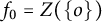 $f_0=Z(\{o\})$
is
$f_0=Z(\{o\})$
is
 $\mathrm {GL}(2,\mathbb Z)$
invariant, and hence almost everywhere constant.
$\mathrm {GL}(2,\mathbb Z)$
invariant, and hence almost everywhere constant.
6 Characterization of
$Z([o,e_1])=f_1$
, and the proof of Theorem 5

According to Lemma 9 and Proposition 11, for an
 $f_1\in \mathcal {M}(\mathbb R^2)$
, there exists a
$f_1\in \mathcal {M}(\mathbb R^2)$
, there exists a
 $\mathcal {G}(\mathbb Z^2)$
covariant valuation
$\mathcal {G}(\mathbb Z^2)$
covariant valuation
 $Z:\mathcal {P}(\mathbb Z^2)\to \mathcal {M}(\mathbb R^2)$
satisfying
$Z:\mathcal {P}(\mathbb Z^2)\to \mathcal {M}(\mathbb R^2)$
satisfying
 $Z([o,e_1])=f_1$
if and only if for any
$Z([o,e_1])=f_1$
if and only if for any
 $(x,y)\in \mathbb R^2$
, we have
$(x,y)\in \mathbb R^2$
, we have
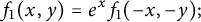 $$ \begin{align} f_1(x,y)&= e^{x}f_1(-x,-y); \end{align} $$
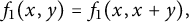 $$ \begin{align}\kern-7pt f_1(x,y)&= f_1(x,x+y), \end{align} $$
 $$ \begin{align}\kern-15pt f_1(x,y)&= f_1(x,-y). \end{align} $$
Proposition 19 For
 $\Omega _{1}=\{(0,y):y\geq 0\}\cup \{(x,y):0\leq y\leq \frac 12\,x\}$
, and for any measurable
$\Omega _{1}=\{(0,y):y\geq 0\}\cup \{(x,y):0\leq y\leq \frac 12\,x\}$
, and for any measurable
 $\tilde {f}_1:\Omega _{1}\to \mathbb R$
, there exists a unique
$\tilde {f}_1:\Omega _{1}\to \mathbb R$
, there exists a unique
 $f_1\in \mathcal {M}(\mathbb R^2)$
satisfying (40)–(42) and
$f_1\in \mathcal {M}(\mathbb R^2)$
satisfying (40)–(42) and
 $f_1|_{\Omega _{1}}=\tilde {f}_1$
.
$f_1|_{\Omega _{1}}=\tilde {f}_1$
.
Proof The key observation is that (41) yields that
 $$ \begin{align} f_1(x,y)=f_1(x,kx+y)\text{ \ for } k\in\mathbb Z \text{ and } x,y\in\mathbb R. \end{align} $$
Now knowing
 $f_1$
on
$f_1$
on
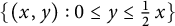 $\{(x,y):0\leq y\leq \frac 12\,x\}$
determines
$\{(x,y):0\leq y\leq \frac 12\,x\}$
determines
 $f_1(x,y)$
for
$f_1(x,y)$
for
 $x>0$
and
$x>0$
and
 $|y|\leq \frac 12\,x$
via (42). We observe that
$|y|\leq \frac 12\,x$
via (42). We observe that
 $$ \begin{align} f_1\left(x,-{\frac12\,}x\right)=f_1\left(x,{\frac12\,}x\right) \text{ \ for } x>0. \end{align} $$
Next knowing
 $f_1$
on
$f_1$
on
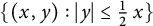 $\{(x,y):|y|\leq \frac 12\,x\}$
determines
$\{(x,y):|y|\leq \frac 12\,x\}$
determines
 $f_1(x,y)$
for
$f_1(x,y)$
for
 $x>0$
and
$x>0$
and
 $y\in \mathbb R$
via (43) where (44) ensures that
$y\in \mathbb R$
via (43) where (44) ensures that
 $f_1$
is well-defined. In addition, knowing
$f_1$
is well-defined. In addition, knowing
 $f_1$
on
$f_1$
on
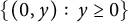 $\{(0,y):\,y\geq 0\}$
determines
$\{(0,y):\,y\geq 0\}$
determines
 $f_1(0,y)$
for
$f_1(0,y)$
for
 $y\in \mathbb R$
as (40) implies
$y\in \mathbb R$
as (40) implies
 $f_1(0,-y)=f_1(0,y)$
. Then, knowing
$f_1(0,-y)=f_1(0,y)$
. Then, knowing
 $f_1$
on
$f_1$
on
 $\{(x,y):x> 0\}$
determines
$\{(x,y):x> 0\}$
determines
 $f_1(x,y)$
for
$f_1(x,y)$
for
 $x<0$
and
$x<0$
and
 $y\in \mathbb R$
via (40). Finally, the
$y\in \mathbb R$
via (40). Finally, the
 $f_1$
constructed this way satisfies (40)– (42).
$f_1$
constructed this way satisfies (40)– (42).
7 Toward a geometric characterization of
$Z(T)=f_2$
for simple valuations

According to Lemma 13 and Proposition 14 in Section 4, if
 $Z:\mathcal {P}(\mathbb Z^2)\to \mathcal {M}(\mathbb R^2)$
is a
$Z:\mathcal {P}(\mathbb Z^2)\to \mathcal {M}(\mathbb R^2)$
is a
 $\mathcal {G}(\mathbb Z^2)$
covariant simple valuation, then
$\mathcal {G}(\mathbb Z^2)$
covariant simple valuation, then
 $Z(T)=f_2$
is characterized by the following properties (cf. (32)–(34) in Lemma 13):
$Z(T)=f_2$
is characterized by the following properties (cf. (32)–(34) in Lemma 13):
 $$ \begin{align}\kern-14pt f_2(-x+y,-x)&= e^{-x}f_2(x,y); \end{align} $$
 $$ \begin{align} f_2(x,y)+e^{x+y}f_2(-x,-y)&=f_2(x,x+y)+f_2(x+y,y); \end{align} $$
 $$ \begin{align} f_2(x,y)&= f_2(y,x). \end{align} $$
Next we provide a partially geometric characterization of functions satisfying (45)–(47). As the first step, we concentrate only on the properties (45) and (47). Let
 $$ \begin{align*}\widetilde{\Omega}=\{(x,y)\in\mathbb R^2:\,y\geq x\geq 0\}. \end{align*} $$
We consider the positive hull
 $\mathrm {pos}\{u,v\}=\{\alpha u+\beta v:\alpha ,\beta \geq 0\}$
of
$\mathrm {pos}\{u,v\}=\{\alpha u+\beta v:\alpha ,\beta \geq 0\}$
of
 $u,v\in \mathbb R^2$
.
$u,v\in \mathbb R^2$
.
Lemma 20 Given any measurable function
 $\tilde {f}:\,\widetilde {\Omega }\to \mathbb R$
, there exists a unique measurable
$\tilde {f}:\,\widetilde {\Omega }\to \mathbb R$
, there exists a unique measurable
 $f_2:\,\mathbb R^2\to \mathbb R$
satisfying (45) and (47) extending
$f_2:\,\mathbb R^2\to \mathbb R$
satisfying (45) and (47) extending
 $\tilde {f}$
.
$\tilde {f}$
.
Proof We consider the
 $\Phi \in \mathrm {SL}(n,\mathbb Z)$
defined by
$\Phi \in \mathrm {SL}(n,\mathbb Z)$
defined by
 $$ \begin{align*}\Phi(x,y)=(-x+y,-x), \end{align*} $$
and hence
 $\Phi ^{-1}(x,y)=(-y,x-y)$
, and (45) is equivalent to
$\Phi ^{-1}(x,y)=(-y,x-y)$
, and (45) is equivalent to
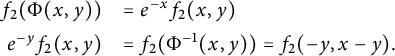 $$ \begin{align} \begin{array}{rl} f_2(\Phi(x,y))&=e^{-x}f_2(x,y)\\[1ex] e^{-y}f_2(x,y)&=f_2(\Phi^{-1}(x,y))=f_2(-y,x-y). \end{array} \end{align} $$
We observe that
 $\Phi $
maps the quadrant
$\Phi $
maps the quadrant
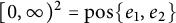 $[0,\infty )^2=\mathrm {pos}\{e_1,e_2\}$
onto
$[0,\infty )^2=\mathrm {pos}\{e_1,e_2\}$
onto
 $\mathrm {pos}\{e_1,-e_1-e_2\}$
, while
$\mathrm {pos}\{e_1,-e_1-e_2\}$
, while
 $\Phi ^{-1}=\Phi ^2$
maps
$\Phi ^{-1}=\Phi ^2$
maps
 $[0,\infty )^2$
onto
$[0,\infty )^2$
onto
 $\mathrm {pos}\{e_2,-e_1-e_2\}$
.
$\mathrm {pos}\{e_2,-e_1-e_2\}$
.
Given a measurable function
 $\tilde {f}:\,\widetilde {\Omega }\to \mathbb R$
, we extend it to an f on
$\tilde {f}:\,\widetilde {\Omega }\to \mathbb R$
, we extend it to an f on
 $[0,\infty )^2$
by setting
$[0,\infty )^2$
by setting
 $f(x,y)=\tilde {f}(y,x)$
if
$f(x,y)=\tilde {f}(y,x)$
if
 $0\leq y\leq x$
. This function satisfies that
$0\leq y\leq x$
. This function satisfies that
 $f(\Phi (x,y))=e^{-x}f(x,y)$
if
$f(\Phi (x,y))=e^{-x}f(x,y)$
if
 $(x,y),\Phi (x,y)\in [0,\infty )^2$
because
$(x,y),\Phi (x,y)\in [0,\infty )^2$
because
 $x=0$
in this case. Using the properties of
$x=0$
in this case. Using the properties of
 $\Phi $
, we can extend f in a unique way to a function
$\Phi $
, we can extend f in a unique way to a function
 $f_2$
on
$f_2$
on
 $\mathbb R^2$
satisfying (48), and hence (45).
$\mathbb R^2$
satisfying (48), and hence (45).
Finally, we need to check whether
 $f_2$
satisfies (47). It does hold on
$f_2$
satisfies (47). It does hold on
 $[0,\infty )^2$
by definition, and the
$[0,\infty )^2$
by definition, and the
 $\Phi [0,\infty )^2$
and
$\Phi [0,\infty )^2$
and
 $\Phi ^{-1}[0,\infty )^2$
are images of each other by the linear transformation
$\Phi ^{-1}[0,\infty )^2$
are images of each other by the linear transformation
 $(x,y)\mapsto (y,x)$
. Therefore, all we need to check is that
$(x,y)\mapsto (y,x)$
. Therefore, all we need to check is that
 $f_2(x,y)=f_2(y,x)$
for
$f_2(x,y)=f_2(y,x)$
for
 $(x,y)\in \Phi ^{-1}[0,\infty )^2$
with
$(x,y)\in \Phi ^{-1}[0,\infty )^2$
with
 $x\neq y$
, and hence
$x\neq y$
, and hence
 $x<0$
and
$x<0$
and
 $y>x$
. We have
$y>x$
. We have
 $(x,y)=\Phi ^{-1}(y-x,-x)$
and
$(x,y)=\Phi ^{-1}(y-x,-x)$
and
 $(y,x)=\Phi (-x,y-x)$
, and hence (48) implies
$(y,x)=\Phi (-x,y-x)$
, and hence (48) implies
 $$ \begin{align*} f_2(x,y)&=e^xf(y-x,-x)\\ f_2(y,x)&=e^xf(-x,y-x) \end{align*} $$
where
 $f(y-x,-x)=f(-x,y-x)$
by the construction of f.
$f(y-x,-x)=f(-x,y-x)$
by the construction of f.
Based on Lemma 20, we plan to include the condition (46) in the characterization, and hence we rewrite (46) into forms suiting better the domains in Lemma 20.
Lemma 21 Assuming that
 $f_2:\,\mathbb R^2\to \mathbb R$
satisfies (45) and (47), we have
$f_2:\,\mathbb R^2\to \mathbb R$
satisfies (45) and (47), we have
 $f_2$
also satisfies (46) if and only if for any
$f_2$
also satisfies (46) if and only if for any
 $x,y\in \mathbb R$
, we have
$x,y\in \mathbb R$
, we have
 $$ \begin{align} f_2(x,y)+e^{x}f_2(y-x,y)=f_2(x,x+y)+f_2(y,x+y). \end{align} $$
Proof We observe that using the substitution
 $a=-x+y$
and
$a=-x+y$
and
 $-x=b$
, (45) is equivalent with
$-x=b$
, (45) is equivalent with
 $e^{-b}f_2(a,b)=f_2(-b,a-b)$
, and in turn (45) is equivalent with
$e^{-b}f_2(a,b)=f_2(-b,a-b)$
, and in turn (45) is equivalent with
 $e^{y}f_2(-x,-y)=f_2(y,y-x)$
for any
$e^{y}f_2(-x,-y)=f_2(y,y-x)$
for any
 $x,y\in \mathbb R$
. Therefore, under the condition of symmetry; namely, that f satisfies (47), the condition (45) is equivalent with
$x,y\in \mathbb R$
. Therefore, under the condition of symmetry; namely, that f satisfies (47), the condition (45) is equivalent with
 $e^{x+y}f_2(-x,-y)=e^xf_2(y-x,y)$
for any
$e^{x+y}f_2(-x,-y)=e^xf_2(y-x,y)$
for any
 $x,y\in \mathbb R$
, and then (46) is equivalent to (49).
$x,y\in \mathbb R$
, and then (46) is equivalent to (49).
8 The proof of Theorem 3
Concerning (49), we observe that if
 $(x,y)\in \widetilde {\Omega }$
where
$(x,y)\in \widetilde {\Omega }$
where
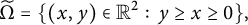 $$ \begin{align*}\widetilde{\Omega}=\{(x,y)\in\mathbb R^2:\,y\geq x\geq 0\}, \end{align*} $$
then
 $(y-x,y)$
,
$(y-x,y)$
,
 $(x,x+y)$
, and
$(x,x+y)$
, and
 $(y,x+y)$
all lie in
$(y,x+y)$
all lie in
 $\widetilde {\Omega }$
. Therefore, it makes sense to consider (49) as a property of a function on
$\widetilde {\Omega }$
. Therefore, it makes sense to consider (49) as a property of a function on
 $\widetilde {\Omega }$
.
$\widetilde {\Omega }$
.
Proposition 22 Given any measurable function
 $\tilde {f}:\,\widetilde {\Omega }\to \mathbb R$
satisfying (49), there exists a unique measurable
$\tilde {f}:\,\widetilde {\Omega }\to \mathbb R$
satisfying (49), there exists a unique measurable
 $f_2:\,\mathbb R^2\to \mathbb R$
satisfying (45)–(47) extending
$f_2:\,\mathbb R^2\to \mathbb R$
satisfying (45)–(47) extending
 $\tilde {f}$
.
$\tilde {f}$
.
Proof Using Lemma 20, first we extend
 $\tilde {f}$
to the unique measurable function
$\tilde {f}$
to the unique measurable function
 $f_2$
on
$f_2$
on
 $\mathbb R^2$
satisfying (45) and (47), and we use (45) in both forms
$\mathbb R^2$
satisfying (45) and (47), and we use (45) in both forms
 $$ \begin{align} e^{-a}f_2(a,b)=f_2(-a+b,-a)\text{ and }e^{-b}f_2(a,b)=f_2(-b,a-b). \end{align} $$
We note that for
 $f_2$
, the formulas
$f_2$
, the formulas
 $f_2(a,b)=f_2(b,a)$
and (50) yield
$f_2(a,b)=f_2(b,a)$
and (50) yield
 $$ \begin{align} \nonumber f_2(x,y)+e^{x}f_2(y-x,y)&=f_2(y,x)+e^{x}e^{y-x}f_2(x,x-y)\\ &=f_2(y,x)+e^{y}f_2(x-y,x). \end{align} $$
Now we verify that
 $f_2$
satisfies (49) for any
$f_2$
satisfies (49) for any
 $x,y\in \mathbb R$
.
$x,y\in \mathbb R$
.
Case 1
 $x,y\geq 0$
If
$x,y\geq 0$
If
 $y\geq x$
, then
$y\geq x$
, then
 $(x,y)\in \widetilde {\Omega }$
, and (49) holds. If
$(x,y)\in \widetilde {\Omega }$
, and (49) holds. If
 $0\leq y<x$
, then combining (49) for
$0\leq y<x$
, then combining (49) for
 $(y,x)\in \widetilde {\Omega }$
and (51) implies (49) again.
$(y,x)\in \widetilde {\Omega }$
and (51) implies (49) again.
Case 2
 $x\leq 0$
and
$x\leq 0$
and
 $y\geq 0$
Now
$y\geq 0$
Now
 $(-x,y)\in [0,\infty )^2$
; therefore, Case 1 yields that
$(-x,y)\in [0,\infty )^2$
; therefore, Case 1 yields that
 $$ \begin{align*}f_2(-x,y)+e^{-x}f_2(y+x,y)=f_2(-x,y-x)+f_2(y,y-x). \end{align*} $$
We multiply through by
 $e^x$
, and observe that (50) and
$e^x$
, and observe that (50) and
 $f_2(a,b)=f_2(b,a)$
imply
$f_2(a,b)=f_2(b,a)$
imply
 $$ \begin{align*}e^{x}f_2(-x,y)+f_2(y+x,y)=f_2(x+y,x)+f_2(y+x,y)=f_2(x,x+y)+f_2(y,y+x), \end{align*} $$
which is the right-hand side of (49). On the other hand, again (50) and
 $f_2(a,b)=f_2(b,a)$
yield
$f_2(a,b)=f_2(b,a)$
yield
 $$ \begin{align*}e^xf_2(-x,y-x)+e^xf_2(y,y-x) &=f_2(y,x)+e^xf_2(y,y-x) \\ &=f_2(x,y)+e^xf_2(y-x,y), \end{align*} $$
which is the left-hand side of (49). In turn, we conclude (49).
Case 3
 $x\geq 0$
and
$x\geq 0$
and
 $y\leq 0$
Now Case 2 yields that
$y\leq 0$
Now Case 2 yields that
 $$ \begin{align*}f_2(y,x)+e^{y}f_2(x-y,x)=f_2(y,y+x)+f_2(x,y+x), \end{align*} $$
Case 4
 $x,y< 0$
As
$x,y< 0$
As
 $-x> 0$
and
$-x> 0$
and
 $y<0$
, Case 3 yields that
$y<0$
, Case 3 yields that
 $$ \begin{align*}f_2(-x,y)+e^{-x}f_2(y+x,y)=f_2(-x,y-x)+f_2(y,y-x). \end{align*} $$
Therefore, the argument in Case 2 yields (49).
According to Proposition 22, the task to construct a measurable function
 $f_2:\,\mathbb R^2\to \mathbb R$
satisfying (45)–(47) – that is needed for Theorem 3 by Lemma 13 and Proposition 14 – is equivalent to construct a measurable function
$f_2:\,\mathbb R^2\to \mathbb R$
satisfying (45)–(47) – that is needed for Theorem 3 by Lemma 13 and Proposition 14 – is equivalent to construct a measurable function
 $\tilde {f}:\,\widetilde {\Omega }\to \mathbb R$
satisfying
$\tilde {f}:\,\widetilde {\Omega }\to \mathbb R$
satisfying
 $$ \begin{align} \tilde{f}(x,y)+e^{x}\tilde{f}(y-x,y)=\tilde{f}(x,x+y)+\tilde{f}(y,x+y). \end{align} $$
When we write
 $\varphi (t)=\frac {e^t-1}{t}$
in the formulas below, we mean the positive analytic function on
$\varphi (t)=\frac {e^t-1}{t}$
in the formulas below, we mean the positive analytic function on
 $\mathbb R$
with
$\mathbb R$
with
 $\varphi (0)=1$
; namely,
$\varphi (0)=1$
; namely,
 $\varphi (t)=\sum _{n=0}^\infty \frac {t^n}{(n+1)!}$
, and hence the reciprocal of
$\varphi (t)=\sum _{n=0}^\infty \frac {t^n}{(n+1)!}$
, and hence the reciprocal of
 $\varphi $
is the series defining the Bernoulli numbers
$\varphi $
is the series defining the Bernoulli numbers
 $B_0, B_1,\ldots $
by the formula (cf. Zagier [Reference Zagier18])
$B_0, B_1,\ldots $
by the formula (cf. Zagier [Reference Zagier18])
 $$ \begin{align*}\frac{t}{e^t-1}=\sum_{n=0}^\infty\frac{B_n}{n!}\cdot t^n. \end{align*} $$
The following statement follows by direct calculations.
Lemma 23 A natural bijection between measurable functions
 $\tilde {f}:\,\widetilde {\Omega }\to \mathbb R$
satisfying (52) and
$\tilde {f}:\,\widetilde {\Omega }\to \mathbb R$
satisfying (52) and
 $\varrho :\,[0,\infty )^2\to \mathbb R$
satisfying (54) is induced by (53) and (55) as follows:
$\varrho :\,[0,\infty )^2\to \mathbb R$
satisfying (54) is induced by (53) and (55) as follows:
-
(i) If a measurable function
$\tilde {f}:\,\widetilde {\Omega }\to \mathbb R$
satisfies (52), then the function
$\varrho :\,[0,\infty )^2\to \mathbb R$
defined by (53)satisfies
$$ \begin{align} \varrho(x,y)=\frac{x}{e^x-1}\cdot \frac{x+y}{e^{x+y}-1}\cdot \left(\tilde{f}(x,x+y)+e^x\cdot \tilde{f}(y,x+y)\right) \end{align} $$
(54)
$$ \begin{align} (2x+y) \varrho(x,y)=(x+y)\varrho(x,x+y)+x \varrho(x+y,x), \end{align} $$
$\varrho (0,0)=2\tilde {f}(0,0)$
, and for
$(x,y)\in \widetilde {\Omega }\backslash (0,0)$
, the formula (55)
$$ \begin{align} \tilde{f}(x,y)=\frac{e^x}{y}\cdot \frac{e^{y-x}-1}{y-x}\cdot \varrho(y-x,x)- \frac{1}y\cdot \frac{e^{x}-1}{x}\cdot \varrho(x,y-x). \end{align} $$
-
(ii) If a function
$\varrho :\,[0,\infty )^2\to \mathbb R$
satisfies (54), then the function
$\tilde {f}:\,\widetilde {\Omega }\to \mathbb R$
defined by (55) satisfies (52).


Remark. The case when the original simple valuation is the positive Laplace transform is equivalent with the property that
 $\varrho $
is the constant
$\varrho $
is the constant
 $1$
function in (54) (cf. (20)).
$1$
function in (54) (cf. (20)).
Proof Substituting the formula (55) for
 $\tilde {f}$
into the left side of (52) results in the expression
$\tilde {f}$
into the left side of (52) results in the expression
 $\frac {(e^x - 1)(e^y - 1)}{xy} \varrho (x,y-x)$
, and into the right-hand side of (52) results in the expression
$\frac {(e^x - 1)(e^y - 1)}{xy} \varrho (x,y-x)$
, and into the right-hand side of (52) results in the expression
 $$ \begin{align*}\frac{(e^x - 1)(e^y - 1)}{xy(x+y)}(y\varrho(x,y) + x \varrho (y,x)). \end{align*} $$
It follows that
 $$ \begin{align*}y\varrho(x,y) + x \varrho (y,x) = (x+y)\varrho(x,y-x), \end{align*} $$
which is equivalent to (54) by replacing y by
 $y-x$
. This proves (ii), and (i) can be verified analogously.
$y-x$
. This proves (ii), and (i) can be verified analogously.
To provide a characterization of the measurable function
 $\varrho :\,[0,\infty )^2\to \mathbb R$
in Lemma 23, we consider the golden ratio
$\varrho :\,[0,\infty )^2\to \mathbb R$
in Lemma 23, we consider the golden ratio
 $$ \begin{align*}\tau=\frac{\sqrt{5}+1}2, \end{align*} $$
which satisfies the properties
 $$ \begin{align} \tau^2=1+\tau\text{ and } \frac1{\tau}=\tau-1\text{ and } \frac{1+\tau}{\tau}=\tau. \end{align} $$
In addition, recall that
 $$ \begin{align} \widetilde{\Omega}_{2}=\{(\tau s,s):1\leq s<\tau\}\cup \{(x,y):0\leq x\leq y\}. \end{align} $$
Lemma 24 If
 $\tilde {\varrho }$
is any (or Lebesgue measurable, or Borel measurable) function on
$\tilde {\varrho }$
is any (or Lebesgue measurable, or Borel measurable) function on
 $\widetilde {\Omega }_2$
into a real vectorspace, then there exists a unique (Lebesgue measurable, or Borel measurable) function
$\widetilde {\Omega }_2$
into a real vectorspace, then there exists a unique (Lebesgue measurable, or Borel measurable) function
 $\varrho $
on
$\varrho $
on
 $[0,\infty )^2$
satisfying
$[0,\infty )^2$
satisfying
 $$ \begin{align} (2x+y) \varrho(x,y)=(x+y)\varrho(x,x+y)+x \varrho(x+y,x), \end{align} $$
whose restriction to
 $\widetilde {\Omega }_2$
is
$\widetilde {\Omega }_2$
is
 $\tilde {\varrho }$
.
$\tilde {\varrho }$
.
Proof If
 $x=0$
and
$x=0$
and
 $y\geq 0$
, then both the left-hand side and the right-hand side of (58) is
$y\geq 0$
, then both the left-hand side and the right-hand side of (58) is
 $y\varrho (0,y)$
, thus (58) provides no restriction on
$y\varrho (0,y)$
, thus (58) provides no restriction on
 $\varrho $
. If
$\varrho $
. If
 $x>0$
and
$x>0$
and
 $y=0$
, then (58) reads as
$y=0$
, then (58) reads as
 $2x\varrho (x,0)=2x\varrho (x,x)$
; therefore,
$2x\varrho (x,0)=2x\varrho (x,x)$
; therefore,
 $\varrho (x,0)=\varrho (x,x)$
. In particular, we may assume that
$\varrho (x,0)=\varrho (x,x)$
. In particular, we may assume that
 $x,y>0$
for
$x,y>0$
for
 $(x,y)\in \widetilde {\Omega }_{2}$
in (58). Since then
$(x,y)\in \widetilde {\Omega }_{2}$
in (58). Since then
 $(x+y,x)\not \in \widetilde {\Omega }_{2}$
, (58) provides no restriction on
$(x+y,x)\not \in \widetilde {\Omega }_{2}$
, (58) provides no restriction on
 $\tilde {\varrho }$
on
$\tilde {\varrho }$
on
 $\widetilde {\Omega }_{2}$
. However, we still need to define
$\widetilde {\Omega }_{2}$
. However, we still need to define
 $\varrho $
on
$\varrho $
on
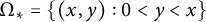 $\Omega _*=\{(x,y):0<y<x\}$
.
$\Omega _*=\{(x,y):0<y<x\}$
.
We recall the Fibonacci sequence, which we index as
 $$ \begin{align*}F_0=0, \text{ and } F_1=1, \text{ and } F_{n+2}=F_n+F_{n+1} \text{ for } n\geq 0. \end{align*} $$
For
 $n\geq 0$
, setting
$n\geq 0$
, setting
 $\frac 1{0}=\infty $
, the Fibonacci sequence (cf. Burton [Reference Burton6]) satisfies
$\frac 1{0}=\infty $
, the Fibonacci sequence (cf. Burton [Reference Burton6]) satisfies
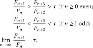 $$ \begin{align*} \frac{F_{n+1}}{F_{n}}&>\frac{F_{n+3}}{F_{n+2}}>\tau \text {if } n\geq 0 \text{ even};\\ \frac{F_{n+1}}{F_{n}}&< \frac{F_{n+3}}{F_{n+2}}<\tau \text {if } n\geq 1 \text{ odd;}\\ \lim_{n\to\infty}\frac{F_{n+1}}{F_{n}}&=\tau. \end{align*} $$
In particular, for
 $n\geq 0$
, we can define
$n\geq 0$
, we can define
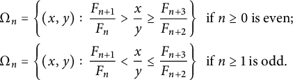 $$ \begin{align*} \Omega_n&=\left\{(x,y):\, \frac{F_{n+1}}{F_{n}}>\frac{x}{y}\geq \frac{F_{n+3}}{F_{n+2}}\right\} \ \text{if } n\geq 0 \text{ is even};\\
\Omega_n&=\left\{(x,y):\, \frac{F_{n+1}}{F_{n}}< \frac{x}{y}\leq \frac{F_{n+3}}{F_{n+2}}\right\} \ \text{if } n\geq 1 \text{ is odd.} \end{align*} $$
$$ \begin{align*} \Omega_n&=\left\{(x,y):\, \frac{F_{n+1}}{F_{n}}>\frac{x}{y}\geq \frac{F_{n+3}}{F_{n+2}}\right\} \ \text{if } n\geq 0 \text{ is even};\\
\Omega_n&=\left\{(x,y):\, \frac{F_{n+1}}{F_{n}}< \frac{x}{y}\leq \frac{F_{n+3}}{F_{n+2}}\right\} \ \text{if } n\geq 1 \text{ is odd.} \end{align*} $$
We observe that
 $\{\Omega _n\}_{n\geq 0}$
is a partition of
$\{\Omega _n\}_{n\geq 0}$
is a partition of
 $\Omega _*\backslash \ell $
for the open half line
$\Omega _*\backslash \ell $
for the open half line
 ${\ell = \{(a,b):\,a=\tau b \text { and }b>0\}}$
by the properties above of the Fibonacci numbers.
${\ell = \{(a,b):\,a=\tau b \text { and }b>0\}}$
by the properties above of the Fibonacci numbers.
We note that for the points of
 $\Omega _*$
and for
$\Omega _*$
and for
 $n\geq 0$
, we have
$n\geq 0$
, we have
 $$ \begin{align} \text{if }(x,y)\in\Omega_*,&\text{ then }\quad (x,x+y)\in\widetilde{\Omega}_{2}; \end{align} $$
 $$ \begin{align} (x,y)\in\Omega_n&\text{ if and only if }\quad (x+y,x)\in\Omega_{n+1} \end{align} $$
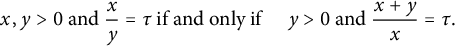 $$ \begin{align} x,y>0\text{ and }\frac{x}{y}=\tau &\text{ if and only if }\quad y>0 \text{ and }\frac{x+y}{x}=\tau. \end{align} $$
We observe that for any
 $x,y$
,
$x,y$
,
 $(x+y,x)\in \Omega _{0}=\{(a,b):a\geq 2b>0\}$
if and only if
$(x+y,x)\in \Omega _{0}=\{(a,b):a\geq 2b>0\}$
if and only if
 $(x,y)\in \{(a,b):0<a\leq b\}\subset \widetilde {\Omega }_{2}$
; therefore, we can define
$(x,y)\in \{(a,b):0<a\leq b\}\subset \widetilde {\Omega }_{2}$
; therefore, we can define
 $\varrho $
on
$\varrho $
on
 $\Omega _0$
via (58). It can be done in a unique way because if
$\Omega _0$
via (58). It can be done in a unique way because if
 $(x,y)\in \Omega _0$
, then
$(x,y)\in \Omega _0$
, then
 $(x+y,x)\in \Omega _{1}$
by (60). Using (59) and (60), we define
$(x+y,x)\in \Omega _{1}$
by (60). Using (59) and (60), we define
 $\varrho $
on any
$\varrho $
on any
 $\Omega _n$
,
$\Omega _n$
,
 $n\geq 0$
, by induction on
$n\geq 0$
, by induction on
 $n\geq 0$
. This extension of
$n\geq 0$
. This extension of
 $\varrho $
onto
$\varrho $
onto
 $\Omega _*\backslash \ell $
is also unique according to (59) and (60). Therefore, all we need to do is to define
$\Omega _*\backslash \ell $
is also unique according to (59) and (60). Therefore, all we need to do is to define
 $\varrho $
on the open half line
$\varrho $
on the open half line
 $\ell $
.
$\ell $
.
For
 $m\in \mathbb Z$
, let
$m\in \mathbb Z$
, let
 $s_m=\{(a,b):\,a=\tau b \text { and }\tau ^m\leq b<\tau ^{m+1}\}\subset \ell $
, and hence
$s_m=\{(a,b):\,a=\tau b \text { and }\tau ^m\leq b<\tau ^{m+1}\}\subset \ell $
, and hence
 $\{s_m\}_{m\in \mathbb Z}$
provides a partition of
$\{s_m\}_{m\in \mathbb Z}$
provides a partition of
 $\ell $
, and
$\ell $
, and
 $\ell \cap \widetilde {\Omega }_{2}=s_0$
. Since
$\ell \cap \widetilde {\Omega }_{2}=s_0$
. Since
 $(x,y)\in s_m$
if and only if
$(x,y)\in s_m$
if and only if
 $(x+y,x)\in s_{m+1}$
according to (61), we can define
$(x+y,x)\in s_{m+1}$
according to (61), we can define
 $\varrho $
on
$\varrho $
on
 $s_n$
for
$s_n$
for
 $n\geq 0$
by induction on n via (58), and similarly we can define
$n\geq 0$
by induction on n via (58), and similarly we can define
 $\varrho $
on
$\varrho $
on
 $s_{-n}$
for
$s_{-n}$
for
 $n\geq 0$
by induction on n again via (58), completing the proof of Lemma 24.
$n\geq 0$
by induction on n again via (58), completing the proof of Lemma 24.
Acknowledgements
We are grateful to Vitaly Bergelson (Ohio State University), Lewis Bowen (University of Texas at Austin), Monika Ludwig (TU Wien), and Árpád Tóth (ELTE) for enlightening discussions. We are grateful for the referee for significantly improving the presentation and the focus of the article.
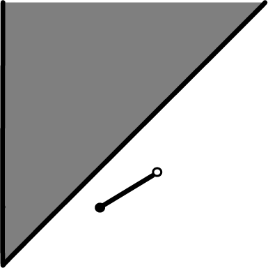

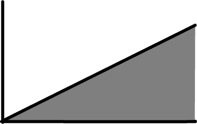


 Open access