


Graph-Based Models for Causal Inference
The graph-based approach to causal inference was primarily formalized by Judea Pearl (Reference Pearl1988, Reference Pearl1995, Reference Pearl2009) and Spirtes, Glymour, and Scheines (Reference Spirtes, Glymour and Scheines2001). A causal graph represents a researcher’s theory about the causal structure of the data-generating mechanism. Based on a causal graph, causal inference can be conducted using the interventional distribution, from which standard causal quantities such as average treatment effects (ATEs) can be derived. In the most general formulation, a causal graph is accompanied by a set of nonparametric structural equations. Thus, a common acronym for Pearl’s general nonparametric model is NPSEM, which stands for non-parametric structural equation model (Pearl, Reference Pearl2009; Shpitser, Richardson, & Robins, Reference Shpitser, Richardson and Robins2020).
Graph-based causal models share many common characteristics with the traditional literature on structural equation models (SEM) prevalent in the social and behavioral sciences and economics (Bollen & Pearl, Reference Bollen and Pearl2013; Heckman & Pinto, Reference Heckman and Pinto2015; Pearl, Reference Pearl2009, Reference Pearl2012). However, these two approaches also differ in several aspects including the underlying assumptions (e.g., graph-based models assume modularity), notational conventions (e.g., the meaning of bidirected edges in graphical representations), research focus (e.g., nonparametric identification in graph-based models vs. parametric estimation in traditional SEM), and standard procedures.
Graph-based procedures often focus on a single causal quantity of interest (e.g., ATE) and establishing its causal identification based on a minimal set of assumptions (e.g., without making parametric assumptions). Causal quantities are well defined via the do-operator and the resulting interventional distribution and causal identification can be established based on graphical tools such as the back-door criterion (Pearl, Reference Pearl1995) or a set of algebraic rules called do-calculus (Shpitser & Pearl, Reference Shpitser and Pearl2006; Tian & Pearl, Reference Tian and Pearl2002a). The central insights developed within the graph-based approach relate to causal identification, whereas less attention has been devoted to the estimation of causal quantities.Footnote 1
On the other hand, the traditional literature on SEM frequently assumes parametrized (often linear) models and usually focuses on identification and estimation of the entire model.Footnote 2 Causal quantities such as direct, indirect and total effects can be defined based on reduced-form equations and partial derivatives (Alwin & Hauser, Reference Alwin and Hauser1975; Bollen, Reference Bollen1987; Stolzenberg, Reference Stolzenberg1980). A main focus within the traditional SEM literature lies on the model implied joint distribution of observed variables and its statistical modeling. A considerable body of literature is available on model identification (Bekker, Merckens, & Wansbeek, Reference Bekker, Merckens and Wansbeek1994; Bollen, Reference Bollen1989; Fisher, Reference Fisher1966; Wiley, Reference Wiley1973) and estimation (Browne, Reference Browne1984; Jöreskog, Reference Jöreskog1967; Satorra & Bentler, Reference Satorra and Bentler1994) for parametrized SEM.
In this paper, we combine causal quantities from graph-based models with identification and estimation results from the traditional literature on linear SEM. For this purpose, we formalize the do-operator using matrix algebra in the section on “Graph-Based Causal Models with Linear Equations.” Based on this matrix representation, we derive a closed-form parametric expression of the interventional distribution and several causal quantities in the section entitled “Interventional Distribution.” Linear graph-based models imply a parametrized joint distribution of the observed variables. We define causal effect functions as a mapping from the parameters of the joint distribution of observed variables onto the causal quantities defined via the do-operator in the section entitled “Causal Effect Functions.” Methods for identifying parametrized causal quantities are discussed in the section entitled “Identification of Parametrized Causal Quantities”. Estimators of causal quantities that are consistent and converge at a rate of
\documentclass[12pt]{minimal}
\usepackage{amsmath}
\usepackage{wasysym}
\usepackage{amsfonts}
\usepackage{amssymb}
\usepackage{amsbsy}
\usepackage{mathrsfs}
\usepackage{upgreek}
\setlength{\oddsidemargin}{-69pt}
\begin{document}$$N^{-1/2}$$\end{document} are proposed in the section on "Estimation of Causal Quantities." We show that the proposed estimators are asymptotically efficient in case of maximum likelihood estimation.
Our work extends the literature on traditional SEM by providing closed-form expressions of graph-based causal quantities in terms of model parameters of linear SEM. Furthermore, we extend the literature on linear graph-based models by providing a unifying estimation framework for (multivariate) causal quantities that also allows estimation of causal quantities beyond the mean and the variance. We illustrate the method using simulated data based on an empirical application and provide a thorough discussion of the differences between conditional and interventional distributions in the illustration section.
Throughout this paper, we focus on situations in which direct causal effects are functionally independent of the values of variables in the system. In other words, direct causal effects are constant. In such situations, the data-generating mechanisms can be adequately represented by linear structural equations and the use of linear graph-based causal models is justified. A priori knowledge that suggests constant direct causal effects sometimes allows identifying causal quantities that would not be identified under the more flexible assumptions of the NPSEM (see illustration section for an example). However, scientific theories that suggest constant direct causal effects might be incorrect and consequently, linear models might be misspecified. We will discuss issues related to model misspecification in the discussion section, where we will also point to future research directions.
Graph-Based Causal Models with Linear Equations
Linear graph-based causal models are an appropriate tool in situations in which a priori scientific knowledge suggests that each of the following statements is true:Footnote 3
-
1. The causal ordering of observed variables and unobserved confounders is known.
-
2. Interventions only alter the mechanisms that are directly targeted (modularity).Footnote 4
-
3. The treatment status of a unit (e.g., person) does not affect the treatment status or the outcome of other units (no interference).
-
4. Direct causal effects are constant across units (homogeneity).
-
5. Direct causal effects are constant across value combinations of observed variables and unobserved error terms (no effect modification).
-
6. Omitted direct causes as comprised in the error terms follow a multivariate normal distribution.Footnote 5
The first three assumptions listed above are generic to the graph-based approach to causal inference and need to hold in its most general nonparametric formulation. Assumptions 4 and 5 justify the use of linear structural equations. Assumptions 6 justifies the use of multivariate normally distributed error terms. We further assume that variables are measured on a continuous scale and are observed without measurement error. Throughout this paper, we assume that the model is correctly specified. In the discussion section, we briefly point to the literature on statistical tests of model assumptions and methods for analyzing the sensitivity of causal conclusions with respect to violations of untestable assumptions. Furthermore, we briefly discuss possible ways to relax the model assumptions (e.g., measurement errors, unobserved heterogeneity, effect modification, excess kurtosis in the error terms).
A linear graph-based causal models over the set
\documentclass[12pt]{minimal}
\usepackage{amsmath}
\usepackage{wasysym}
\usepackage{amsfonts}
\usepackage{amssymb}
\usepackage{amsbsy}
\usepackage{mathrsfs}
\usepackage{upgreek}
\setlength{\oddsidemargin}{-69pt}
\begin{document}$${\mathcal {V}}=\{V_1,...,V_n\}$$\end{document} of observed variables are defined by the following set of equations (Brito & Pearl, Reference Brito and Pearl2006, p.2):Footnote 6

We assume that all variables are deviations from their means and no intercepts are included in Eq. (1). A nonzero structural coefficient (
\documentclass[12pt]{minimal}
\usepackage{amsmath}
\usepackage{wasysym}
\usepackage{amsfonts}
\usepackage{amssymb}
\usepackage{amsbsy}
\usepackage{mathrsfs}
\usepackage{upgreek}
\setlength{\oddsidemargin}{-69pt}
\begin{document}$$c_{ji}\ne 0$$\end{document} ) expresses the assumption that
\documentclass[12pt]{minimal}
\usepackage{amsmath}
\usepackage{wasysym}
\usepackage{amsfonts}
\usepackage{amssymb}
\usepackage{amsbsy}
\usepackage{mathrsfs}
\usepackage{upgreek}
\setlength{\oddsidemargin}{-69pt}
\begin{document}$$V_i$$\end{document}
) expresses the assumption that
\documentclass[12pt]{minimal}
\usepackage{amsmath}
\usepackage{wasysym}
\usepackage{amsfonts}
\usepackage{amssymb}
\usepackage{amsbsy}
\usepackage{mathrsfs}
\usepackage{upgreek}
\setlength{\oddsidemargin}{-69pt}
\begin{document}$$V_i$$\end{document} has a direct causal influence on
\documentclass[12pt]{minimal}
\usepackage{amsmath}
\usepackage{wasysym}
\usepackage{amsfonts}
\usepackage{amssymb}
\usepackage{amsbsy}
\usepackage{mathrsfs}
\usepackage{upgreek}
\setlength{\oddsidemargin}{-69pt}
\begin{document}$$V_j$$\end{document}
has a direct causal influence on
\documentclass[12pt]{minimal}
\usepackage{amsmath}
\usepackage{wasysym}
\usepackage{amsfonts}
\usepackage{amssymb}
\usepackage{amsbsy}
\usepackage{mathrsfs}
\usepackage{upgreek}
\setlength{\oddsidemargin}{-69pt}
\begin{document}$$V_j$$\end{document} . Restricting a structural coefficient to zero (
\documentclass[12pt]{minimal}
\usepackage{amsmath}
\usepackage{wasysym}
\usepackage{amsfonts}
\usepackage{amssymb}
\usepackage{amsbsy}
\usepackage{mathrsfs}
\usepackage{upgreek}
\setlength{\oddsidemargin}{-69pt}
\begin{document}$$c_{ji}=0$$\end{document}
. Restricting a structural coefficient to zero (
\documentclass[12pt]{minimal}
\usepackage{amsmath}
\usepackage{wasysym}
\usepackage{amsfonts}
\usepackage{amssymb}
\usepackage{amsbsy}
\usepackage{mathrsfs}
\usepackage{upgreek}
\setlength{\oddsidemargin}{-69pt}
\begin{document}$$c_{ji}=0$$\end{document} ) indicates the assumption that
\documentclass[12pt]{minimal}
\usepackage{amsmath}
\usepackage{wasysym}
\usepackage{amsfonts}
\usepackage{amssymb}
\usepackage{amsbsy}
\usepackage{mathrsfs}
\usepackage{upgreek}
\setlength{\oddsidemargin}{-69pt}
\begin{document}$$V_i$$\end{document}
) indicates the assumption that
\documentclass[12pt]{minimal}
\usepackage{amsmath}
\usepackage{wasysym}
\usepackage{amsfonts}
\usepackage{amssymb}
\usepackage{amsbsy}
\usepackage{mathrsfs}
\usepackage{upgreek}
\setlength{\oddsidemargin}{-69pt}
\begin{document}$$V_i$$\end{document} has no direct causal effect on
\documentclass[12pt]{minimal}
\usepackage{amsmath}
\usepackage{wasysym}
\usepackage{amsfonts}
\usepackage{amssymb}
\usepackage{amsbsy}
\usepackage{mathrsfs}
\usepackage{upgreek}
\setlength{\oddsidemargin}{-69pt}
\begin{document}$$V_j$$\end{document}
has no direct causal effect on
\documentclass[12pt]{minimal}
\usepackage{amsmath}
\usepackage{wasysym}
\usepackage{amsfonts}
\usepackage{amssymb}
\usepackage{amsbsy}
\usepackage{mathrsfs}
\usepackage{upgreek}
\setlength{\oddsidemargin}{-69pt}
\begin{document}$$V_j$$\end{document} . The parameter
\documentclass[12pt]{minimal}
\usepackage{amsmath}
\usepackage{wasysym}
\usepackage{amsfonts}
\usepackage{amssymb}
\usepackage{amsbsy}
\usepackage{mathrsfs}
\usepackage{upgreek}
\setlength{\oddsidemargin}{-69pt}
\begin{document}$$c_{ji}$$\end{document}
. The parameter
\documentclass[12pt]{minimal}
\usepackage{amsmath}
\usepackage{wasysym}
\usepackage{amsfonts}
\usepackage{amssymb}
\usepackage{amsbsy}
\usepackage{mathrsfs}
\usepackage{upgreek}
\setlength{\oddsidemargin}{-69pt}
\begin{document}$$c_{ji}$$\end{document} quantifies the magnitude of a direct effect. The
\documentclass[12pt]{minimal}
\usepackage{amsmath}
\usepackage{wasysym}
\usepackage{amsfonts}
\usepackage{amssymb}
\usepackage{amsbsy}
\usepackage{mathrsfs}
\usepackage{upgreek}
\setlength{\oddsidemargin}{-69pt}
\begin{document}$$q \times 1$$\end{document}
quantifies the magnitude of a direct effect. The
\documentclass[12pt]{minimal}
\usepackage{amsmath}
\usepackage{wasysym}
\usepackage{amsfonts}
\usepackage{amssymb}
\usepackage{amsbsy}
\usepackage{mathrsfs}
\usepackage{upgreek}
\setlength{\oddsidemargin}{-69pt}
\begin{document}$$q \times 1$$\end{document} parameter vector
\documentclass[12pt]{minimal}
\usepackage{amsmath}
\usepackage{wasysym}
\usepackage{amsfonts}
\usepackage{amssymb}
\usepackage{amsbsy}
\usepackage{mathrsfs}
\usepackage{upgreek}
\setlength{\oddsidemargin}{-69pt}
\begin{document}$${\varvec{\theta }}_{{\mathcal {F}}}\in {\varvec{\Theta }}_{{\mathcal {F}}}\subseteq {\mathbb {R}}^q$$\end{document}
parameter vector
\documentclass[12pt]{minimal}
\usepackage{amsmath}
\usepackage{wasysym}
\usepackage{amsfonts}
\usepackage{amssymb}
\usepackage{amsbsy}
\usepackage{mathrsfs}
\usepackage{upgreek}
\setlength{\oddsidemargin}{-69pt}
\begin{document}$${\varvec{\theta }}_{{\mathcal {F}}}\in {\varvec{\Theta }}_{{\mathcal {F}}}\subseteq {\mathbb {R}}^q$$\end{document} contains all distinct, functionally unrelated and unknown structural coefficients
\documentclass[12pt]{minimal}
\usepackage{amsmath}
\usepackage{wasysym}
\usepackage{amsfonts}
\usepackage{amssymb}
\usepackage{amsbsy}
\usepackage{mathrsfs}
\usepackage{upgreek}
\setlength{\oddsidemargin}{-69pt}
\begin{document}$$c_{ji}$$\end{document}
contains all distinct, functionally unrelated and unknown structural coefficients
\documentclass[12pt]{minimal}
\usepackage{amsmath}
\usepackage{wasysym}
\usepackage{amsfonts}
\usepackage{amssymb}
\usepackage{amsbsy}
\usepackage{mathrsfs}
\usepackage{upgreek}
\setlength{\oddsidemargin}{-69pt}
\begin{document}$$c_{ji}$$\end{document} .
\documentclass[12pt]{minimal}
\usepackage{amsmath}
\usepackage{wasysym}
\usepackage{amsfonts}
\usepackage{amssymb}
\usepackage{amsbsy}
\usepackage{mathrsfs}
\usepackage{upgreek}
\setlength{\oddsidemargin}{-69pt}
\begin{document}$${\varvec{\Theta }}_{{\mathcal {F}}}$$\end{document}
.
\documentclass[12pt]{minimal}
\usepackage{amsmath}
\usepackage{wasysym}
\usepackage{amsfonts}
\usepackage{amssymb}
\usepackage{amsbsy}
\usepackage{mathrsfs}
\usepackage{upgreek}
\setlength{\oddsidemargin}{-69pt}
\begin{document}$${\varvec{\Theta }}_{{\mathcal {F}}}$$\end{document} denotes the parameter space, and it is a subspace of the q-dimensional Euclidean space. Restating Eqs. (1) in matrix notation yields:

The
\documentclass[12pt]{minimal}
\usepackage{amsmath}
\usepackage{wasysym}
\usepackage{amsfonts}
\usepackage{amssymb}
\usepackage{amsbsy}
\usepackage{mathrsfs}
\usepackage{upgreek}
\setlength{\oddsidemargin}{-69pt}
\begin{document}$$n \times n$$\end{document} identity matrix is denoted as
\documentclass[12pt]{minimal}
\usepackage{amsmath}
\usepackage{wasysym}
\usepackage{amsfonts}
\usepackage{amssymb}
\usepackage{amsbsy}
\usepackage{mathrsfs}
\usepackage{upgreek}
\setlength{\oddsidemargin}{-69pt}
\begin{document}$${\mathbf{I}}_n$$\end{document}
identity matrix is denoted as
\documentclass[12pt]{minimal}
\usepackage{amsmath}
\usepackage{wasysym}
\usepackage{amsfonts}
\usepackage{amssymb}
\usepackage{amsbsy}
\usepackage{mathrsfs}
\usepackage{upgreek}
\setlength{\oddsidemargin}{-69pt}
\begin{document}$${\mathbf{I}}_n$$\end{document} . The
\documentclass[12pt]{minimal}
\usepackage{amsmath}
\usepackage{wasysym}
\usepackage{amsfonts}
\usepackage{amssymb}
\usepackage{amsbsy}
\usepackage{mathrsfs}
\usepackage{upgreek}
\setlength{\oddsidemargin}{-69pt}
\begin{document}$$n \times n$$\end{document}
. The
\documentclass[12pt]{minimal}
\usepackage{amsmath}
\usepackage{wasysym}
\usepackage{amsfonts}
\usepackage{amssymb}
\usepackage{amsbsy}
\usepackage{mathrsfs}
\usepackage{upgreek}
\setlength{\oddsidemargin}{-69pt}
\begin{document}$$n \times n$$\end{document} matrix of structural coefficients is denoted as
\documentclass[12pt]{minimal}
\usepackage{amsmath}
\usepackage{wasysym}
\usepackage{amsfonts}
\usepackage{amssymb}
\usepackage{amsbsy}
\usepackage{mathrsfs}
\usepackage{upgreek}
\setlength{\oddsidemargin}{-69pt}
\begin{document}$${\mathbf {C}}$$\end{document}
matrix of structural coefficients is denoted as
\documentclass[12pt]{minimal}
\usepackage{amsmath}
\usepackage{wasysym}
\usepackage{amsfonts}
\usepackage{amssymb}
\usepackage{amsbsy}
\usepackage{mathrsfs}
\usepackage{upgreek}
\setlength{\oddsidemargin}{-69pt}
\begin{document}$${\mathbf {C}}$$\end{document} , and we sometimes use the notation
\documentclass[12pt]{minimal}
\usepackage{amsmath}
\usepackage{wasysym}
\usepackage{amsfonts}
\usepackage{amssymb}
\usepackage{amsbsy}
\usepackage{mathrsfs}
\usepackage{upgreek}
\setlength{\oddsidemargin}{-69pt}
\begin{document}$${\mathbf {C}}({\varvec{\theta }}_{{\mathcal {F}}})$$\end{document}
, and we sometimes use the notation
\documentclass[12pt]{minimal}
\usepackage{amsmath}
\usepackage{wasysym}
\usepackage{amsfonts}
\usepackage{amssymb}
\usepackage{amsbsy}
\usepackage{mathrsfs}
\usepackage{upgreek}
\setlength{\oddsidemargin}{-69pt}
\begin{document}$${\mathbf {C}}({\varvec{\theta }}_{{\mathcal {F}}})$$\end{document} to emphasize that
\documentclass[12pt]{minimal}
\usepackage{amsmath}
\usepackage{wasysym}
\usepackage{amsfonts}
\usepackage{amssymb}
\usepackage{amsbsy}
\usepackage{mathrsfs}
\usepackage{upgreek}
\setlength{\oddsidemargin}{-69pt}
\begin{document}$${\mathbf {C}}$$\end{document}
to emphasize that
\documentclass[12pt]{minimal}
\usepackage{amsmath}
\usepackage{wasysym}
\usepackage{amsfonts}
\usepackage{amssymb}
\usepackage{amsbsy}
\usepackage{mathrsfs}
\usepackage{upgreek}
\setlength{\oddsidemargin}{-69pt}
\begin{document}$${\mathbf {C}}$$\end{document} is a function of
\documentclass[12pt]{minimal}
\usepackage{amsmath}
\usepackage{wasysym}
\usepackage{amsfonts}
\usepackage{amssymb}
\usepackage{amsbsy}
\usepackage{mathrsfs}
\usepackage{upgreek}
\setlength{\oddsidemargin}{-69pt}
\begin{document}$${\varvec{\theta }}_{{\mathcal {F}}}$$\end{document}
is a function of
\documentclass[12pt]{minimal}
\usepackage{amsmath}
\usepackage{wasysym}
\usepackage{amsfonts}
\usepackage{amssymb}
\usepackage{amsbsy}
\usepackage{mathrsfs}
\usepackage{upgreek}
\setlength{\oddsidemargin}{-69pt}
\begin{document}$${\varvec{\theta }}_{{\mathcal {F}}}$$\end{document} . We restrict our attention to recursive systems for which the variables
\documentclass[12pt]{minimal}
\usepackage{amsmath}
\usepackage{wasysym}
\usepackage{amsfonts}
\usepackage{amssymb}
\usepackage{amsbsy}
\usepackage{mathrsfs}
\usepackage{upgreek}
\setlength{\oddsidemargin}{-69pt}
\begin{document}$${\mathbf {V}}$$\end{document}
. We restrict our attention to recursive systems for which the variables
\documentclass[12pt]{minimal}
\usepackage{amsmath}
\usepackage{wasysym}
\usepackage{amsfonts}
\usepackage{amssymb}
\usepackage{amsbsy}
\usepackage{mathrsfs}
\usepackage{upgreek}
\setlength{\oddsidemargin}{-69pt}
\begin{document}$${\mathbf {V}}$$\end{document} can be ordered in such a way that the matrix
\documentclass[12pt]{minimal}
\usepackage{amsmath}
\usepackage{wasysym}
\usepackage{amsfonts}
\usepackage{amssymb}
\usepackage{amsbsy}
\usepackage{mathrsfs}
\usepackage{upgreek}
\setlength{\oddsidemargin}{-69pt}
\begin{document}$${\mathbf {C}}$$\end{document}
can be ordered in such a way that the matrix
\documentclass[12pt]{minimal}
\usepackage{amsmath}
\usepackage{wasysym}
\usepackage{amsfonts}
\usepackage{amssymb}
\usepackage{amsbsy}
\usepackage{mathrsfs}
\usepackage{upgreek}
\setlength{\oddsidemargin}{-69pt}
\begin{document}$${\mathbf {C}}$$\end{document} is strictly lower triangular (which ensures the existence of the inverse in Eq. (2); Bollen, Reference Bollen1989). The set of error terms is denoted by
\documentclass[12pt]{minimal}
\usepackage{amsmath}
\usepackage{wasysym}
\usepackage{amsfonts}
\usepackage{amssymb}
\usepackage{amsbsy}
\usepackage{mathrsfs}
\usepackage{upgreek}
\setlength{\oddsidemargin}{-69pt}
\begin{document}$${\mathcal {E}}=\{\varepsilon _1,...,\varepsilon _n\}$$\end{document}
is strictly lower triangular (which ensures the existence of the inverse in Eq. (2); Bollen, Reference Bollen1989). The set of error terms is denoted by
\documentclass[12pt]{minimal}
\usepackage{amsmath}
\usepackage{wasysym}
\usepackage{amsfonts}
\usepackage{amssymb}
\usepackage{amsbsy}
\usepackage{mathrsfs}
\usepackage{upgreek}
\setlength{\oddsidemargin}{-69pt}
\begin{document}$${\mathcal {E}}=\{\varepsilon _1,...,\varepsilon _n\}$$\end{document} . Each error term
\documentclass[12pt]{minimal}
\usepackage{amsmath}
\usepackage{wasysym}
\usepackage{amsfonts}
\usepackage{amssymb}
\usepackage{amsbsy}
\usepackage{mathrsfs}
\usepackage{upgreek}
\setlength{\oddsidemargin}{-69pt}
\begin{document}$$\varepsilon _i$$\end{document}
. Each error term
\documentclass[12pt]{minimal}
\usepackage{amsmath}
\usepackage{wasysym}
\usepackage{amsfonts}
\usepackage{amssymb}
\usepackage{amsbsy}
\usepackage{mathrsfs}
\usepackage{upgreek}
\setlength{\oddsidemargin}{-69pt}
\begin{document}$$\varepsilon _i$$\end{document} ,
\documentclass[12pt]{minimal}
\usepackage{amsmath}
\usepackage{wasysym}
\usepackage{amsfonts}
\usepackage{amssymb}
\usepackage{amsbsy}
\usepackage{mathrsfs}
\usepackage{upgreek}
\setlength{\oddsidemargin}{-69pt}
\begin{document}$$i=1,...,n$$\end{document}
,
\documentclass[12pt]{minimal}
\usepackage{amsmath}
\usepackage{wasysym}
\usepackage{amsfonts}
\usepackage{amssymb}
\usepackage{amsbsy}
\usepackage{mathrsfs}
\usepackage{upgreek}
\setlength{\oddsidemargin}{-69pt}
\begin{document}$$i=1,...,n$$\end{document} , comprises variables that determine the level of
\documentclass[12pt]{minimal}
\usepackage{amsmath}
\usepackage{wasysym}
\usepackage{amsfonts}
\usepackage{amssymb}
\usepackage{amsbsy}
\usepackage{mathrsfs}
\usepackage{upgreek}
\setlength{\oddsidemargin}{-69pt}
\begin{document}$$V_i$$\end{document}
, comprises variables that determine the level of
\documentclass[12pt]{minimal}
\usepackage{amsmath}
\usepackage{wasysym}
\usepackage{amsfonts}
\usepackage{amssymb}
\usepackage{amsbsy}
\usepackage{mathrsfs}
\usepackage{upgreek}
\setlength{\oddsidemargin}{-69pt}
\begin{document}$$V_i$$\end{document} but are not explicitly included in the model. Typically the following assumptions (or a subset thereof) are made (Brito & Pearl, Reference Brito and Pearl2002; Kang & Tian, Reference Kang and Tian2009; Koster, Reference Koster1999):
-
(a) \documentclass[12pt]{minimal} \usepackage{amsmath} \usepackage{wasysym} \usepackage{amsfonts} \usepackage{amssymb} \usepackage{amsbsy} \usepackage{mathrsfs} \usepackage{upgreek} \setlength{\oddsidemargin}{-69pt} \begin{document}$$\mathrm {E}({\varvec{\varepsilon }})={\mathbf {0}}_n$$\end{document}
 , where
\documentclass[12pt]{minimal}
\usepackage{amsmath}
\usepackage{wasysym}
\usepackage{amsfonts}
\usepackage{amssymb}
\usepackage{amsbsy}
\usepackage{mathrsfs}
\usepackage{upgreek}
\setlength{\oddsidemargin}{-69pt}
\begin{document}$${\mathbf {0}}_n$$\end{document} is an
\documentclass[12pt]{minimal}
\usepackage{amsmath}
\usepackage{wasysym}
\usepackage{amsfonts}
\usepackage{amssymb}
\usepackage{amsbsy}
\usepackage{mathrsfs}
\usepackage{upgreek}
\setlength{\oddsidemargin}{-69pt}
\begin{document}$$n\times 1$$\end{document} vector that contains only zeros.
, where
\documentclass[12pt]{minimal}
\usepackage{amsmath}
\usepackage{wasysym}
\usepackage{amsfonts}
\usepackage{amssymb}
\usepackage{amsbsy}
\usepackage{mathrsfs}
\usepackage{upgreek}
\setlength{\oddsidemargin}{-69pt}
\begin{document}$${\mathbf {0}}_n$$\end{document} is an
\documentclass[12pt]{minimal}
\usepackage{amsmath}
\usepackage{wasysym}
\usepackage{amsfonts}
\usepackage{amssymb}
\usepackage{amsbsy}
\usepackage{mathrsfs}
\usepackage{upgreek}
\setlength{\oddsidemargin}{-69pt}
\begin{document}$$n\times 1$$\end{document} vector that contains only zeros. -
(b) \documentclass[12pt]{minimal} \usepackage{amsmath} \usepackage{wasysym} \usepackage{amsfonts} \usepackage{amssymb} \usepackage{amsbsy} \usepackage{mathrsfs} \usepackage{upgreek} \setlength{\oddsidemargin}{-69pt} \begin{document}$$\mathrm {E}({\varvec{\varepsilon }}{\varvec{\varepsilon }}^\intercal )={\varvec{\Psi }}$$\end{document}
, where the
\documentclass[12pt]{minimal}
\usepackage{amsmath}
\usepackage{wasysym}
\usepackage{amsfonts}
\usepackage{amssymb}
\usepackage{amsbsy}
\usepackage{mathrsfs}
\usepackage{upgreek}
\setlength{\oddsidemargin}{-69pt}
\begin{document}$$n\times n$$\end{document} matrix
\documentclass[12pt]{minimal}
\usepackage{amsmath}
\usepackage{wasysym}
\usepackage{amsfonts}
\usepackage{amssymb}
\usepackage{amsbsy}
\usepackage{mathrsfs}
\usepackage{upgreek}
\setlength{\oddsidemargin}{-69pt}
\begin{document}$${\varvec{\Psi }}$$\end{document} is finite, symmetric and positive definite. -
(c) \documentclass[12pt]{minimal} \usepackage{amsmath} \usepackage{wasysym} \usepackage{amsfonts} \usepackage{amssymb} \usepackage{amsbsy} \usepackage{mathrsfs} \usepackage{upgreek} \setlength{\oddsidemargin}{-69pt} \begin{document}$${\varvec{\varepsilon }}\sim {{N}}_n({\mathbf {0}}_n,{\varvec{\Psi }})$$\end{document}
, where
\documentclass[12pt]{minimal}
\usepackage{amsmath}
\usepackage{wasysym}
\usepackage{amsfonts}
\usepackage{amssymb}
\usepackage{amsbsy}
\usepackage{mathrsfs}
\usepackage{upgreek}
\setlength{\oddsidemargin}{-69pt}
\begin{document}$${{N}}_n$$\end{document} denotes the n-dimensional normal distribution.


A nonzero covariance
\documentclass[12pt]{minimal}
\usepackage{amsmath}
\usepackage{wasysym}
\usepackage{amsfonts}
\usepackage{amssymb}
\usepackage{amsbsy}
\usepackage{mathrsfs}
\usepackage{upgreek}
\setlength{\oddsidemargin}{-69pt}
\begin{document}$$\psi _{ij}$$\end{document} indicates the existence of an unobserved common cause of the variables
\documentclass[12pt]{minimal}
\usepackage{amsmath}
\usepackage{wasysym}
\usepackage{amsfonts}
\usepackage{amssymb}
\usepackage{amsbsy}
\usepackage{mathrsfs}
\usepackage{upgreek}
\setlength{\oddsidemargin}{-69pt}
\begin{document}$$V_i$$\end{document}
indicates the existence of an unobserved common cause of the variables
\documentclass[12pt]{minimal}
\usepackage{amsmath}
\usepackage{wasysym}
\usepackage{amsfonts}
\usepackage{amssymb}
\usepackage{amsbsy}
\usepackage{mathrsfs}
\usepackage{upgreek}
\setlength{\oddsidemargin}{-69pt}
\begin{document}$$V_i$$\end{document} and
\documentclass[12pt]{minimal}
\usepackage{amsmath}
\usepackage{wasysym}
\usepackage{amsfonts}
\usepackage{amssymb}
\usepackage{amsbsy}
\usepackage{mathrsfs}
\usepackage{upgreek}
\setlength{\oddsidemargin}{-69pt}
\begin{document}$$V_j$$\end{document}
and
\documentclass[12pt]{minimal}
\usepackage{amsmath}
\usepackage{wasysym}
\usepackage{amsfonts}
\usepackage{amssymb}
\usepackage{amsbsy}
\usepackage{mathrsfs}
\usepackage{upgreek}
\setlength{\oddsidemargin}{-69pt}
\begin{document}$$V_j$$\end{document} . The
\documentclass[12pt]{minimal}
\usepackage{amsmath}
\usepackage{wasysym}
\usepackage{amsfonts}
\usepackage{amssymb}
\usepackage{amsbsy}
\usepackage{mathrsfs}
\usepackage{upgreek}
\setlength{\oddsidemargin}{-69pt}
\begin{document}$$p \times 1$$\end{document}
. The
\documentclass[12pt]{minimal}
\usepackage{amsmath}
\usepackage{wasysym}
\usepackage{amsfonts}
\usepackage{amssymb}
\usepackage{amsbsy}
\usepackage{mathrsfs}
\usepackage{upgreek}
\setlength{\oddsidemargin}{-69pt}
\begin{document}$$p \times 1$$\end{document} parameter vector
\documentclass[12pt]{minimal}
\usepackage{amsmath}
\usepackage{wasysym}
\usepackage{amsfonts}
\usepackage{amssymb}
\usepackage{amsbsy}
\usepackage{mathrsfs}
\usepackage{upgreek}
\setlength{\oddsidemargin}{-69pt}
\begin{document}$${\varvec{\theta }}_{{\mathcal {P}}}\in {\varvec{\Theta }}_{{\mathcal {P}}}\subseteq {\mathbb {R}}^p$$\end{document}
parameter vector
\documentclass[12pt]{minimal}
\usepackage{amsmath}
\usepackage{wasysym}
\usepackage{amsfonts}
\usepackage{amssymb}
\usepackage{amsbsy}
\usepackage{mathrsfs}
\usepackage{upgreek}
\setlength{\oddsidemargin}{-69pt}
\begin{document}$${\varvec{\theta }}_{{\mathcal {P}}}\in {\varvec{\Theta }}_{{\mathcal {P}}}\subseteq {\mathbb {R}}^p$$\end{document} contains all distinct, functionally unrelated and unknown parameters from the error term distribution.
\documentclass[12pt]{minimal}
\usepackage{amsmath}
\usepackage{wasysym}
\usepackage{amsfonts}
\usepackage{amssymb}
\usepackage{amsbsy}
\usepackage{mathrsfs}
\usepackage{upgreek}
\setlength{\oddsidemargin}{-69pt}
\begin{document}$${\varvec{\Theta }}_{{\mathcal {P}}}$$\end{document}
contains all distinct, functionally unrelated and unknown parameters from the error term distribution.
\documentclass[12pt]{minimal}
\usepackage{amsmath}
\usepackage{wasysym}
\usepackage{amsfonts}
\usepackage{amssymb}
\usepackage{amsbsy}
\usepackage{mathrsfs}
\usepackage{upgreek}
\setlength{\oddsidemargin}{-69pt}
\begin{document}$${\varvec{\Theta }}_{{\mathcal {P}}}$$\end{document} denotes the parameter space, and it is a subspace of the p-dimensional Euclidean space. We sometimes use the notation
\documentclass[12pt]{minimal}
\usepackage{amsmath}
\usepackage{wasysym}
\usepackage{amsfonts}
\usepackage{amssymb}
\usepackage{amsbsy}
\usepackage{mathrsfs}
\usepackage{upgreek}
\setlength{\oddsidemargin}{-69pt}
\begin{document}$${\varvec{\Psi }}({\varvec{\theta }}_{{\mathcal {P}}})$$\end{document}
denotes the parameter space, and it is a subspace of the p-dimensional Euclidean space. We sometimes use the notation
\documentclass[12pt]{minimal}
\usepackage{amsmath}
\usepackage{wasysym}
\usepackage{amsfonts}
\usepackage{amssymb}
\usepackage{amsbsy}
\usepackage{mathrsfs}
\usepackage{upgreek}
\setlength{\oddsidemargin}{-69pt}
\begin{document}$${\varvec{\Psi }}({\varvec{\theta }}_{{\mathcal {P}}})$$\end{document} to emphasize that
\documentclass[12pt]{minimal}
\usepackage{amsmath}
\usepackage{wasysym}
\usepackage{amsfonts}
\usepackage{amssymb}
\usepackage{amsbsy}
\usepackage{mathrsfs}
\usepackage{upgreek}
\setlength{\oddsidemargin}{-69pt}
\begin{document}$${\varvec{\Psi }}$$\end{document}
to emphasize that
\documentclass[12pt]{minimal}
\usepackage{amsmath}
\usepackage{wasysym}
\usepackage{amsfonts}
\usepackage{amssymb}
\usepackage{amsbsy}
\usepackage{mathrsfs}
\usepackage{upgreek}
\setlength{\oddsidemargin}{-69pt}
\begin{document}$${\varvec{\Psi }}$$\end{document} is a function of
\documentclass[12pt]{minimal}
\usepackage{amsmath}
\usepackage{wasysym}
\usepackage{amsfonts}
\usepackage{amssymb}
\usepackage{amsbsy}
\usepackage{mathrsfs}
\usepackage{upgreek}
\setlength{\oddsidemargin}{-69pt}
\begin{document}$${\varvec{\theta }}_{{\mathcal {P}}}$$\end{document}
is a function of
\documentclass[12pt]{minimal}
\usepackage{amsmath}
\usepackage{wasysym}
\usepackage{amsfonts}
\usepackage{amssymb}
\usepackage{amsbsy}
\usepackage{mathrsfs}
\usepackage{upgreek}
\setlength{\oddsidemargin}{-69pt}
\begin{document}$${\varvec{\theta }}_{{\mathcal {P}}}$$\end{document} . The resulting model implied joint distribution of the observed variables is denoted by
\documentclass[12pt]{minimal}
\usepackage{amsmath}
\usepackage{wasysym}
\usepackage{amsfonts}
\usepackage{amssymb}
\usepackage{amsbsy}
\usepackage{mathrsfs}
\usepackage{upgreek}
\setlength{\oddsidemargin}{-69pt}
\begin{document}$$\{P({\mathbf {v}},{\varvec{\theta }})\mid {\varvec{\theta }} \in {\varvec{\Theta }}\}$$\end{document}
. The resulting model implied joint distribution of the observed variables is denoted by
\documentclass[12pt]{minimal}
\usepackage{amsmath}
\usepackage{wasysym}
\usepackage{amsfonts}
\usepackage{amssymb}
\usepackage{amsbsy}
\usepackage{mathrsfs}
\usepackage{upgreek}
\setlength{\oddsidemargin}{-69pt}
\begin{document}$$\{P({\mathbf {v}},{\varvec{\theta }})\mid {\varvec{\theta }} \in {\varvec{\Theta }}\}$$\end{document} , where
\documentclass[12pt]{minimal}
\usepackage{amsmath}
\usepackage{wasysym}
\usepackage{amsfonts}
\usepackage{amssymb}
\usepackage{amsbsy}
\usepackage{mathrsfs}
\usepackage{upgreek}
\setlength{\oddsidemargin}{-69pt}
\begin{document}$${\varvec{\Theta }}={\varvec{\Theta }}_{{\mathcal {F}}}\times {\varvec{\Theta }}_{{\mathcal {P}}}$$\end{document}
, where
\documentclass[12pt]{minimal}
\usepackage{amsmath}
\usepackage{wasysym}
\usepackage{amsfonts}
\usepackage{amssymb}
\usepackage{amsbsy}
\usepackage{mathrsfs}
\usepackage{upgreek}
\setlength{\oddsidemargin}{-69pt}
\begin{document}$${\varvec{\Theta }}={\varvec{\Theta }}_{{\mathcal {F}}}\times {\varvec{\Theta }}_{{\mathcal {P}}}$$\end{document} , and P is the family of n-dimensional multivariate normal distributions.
The graph
\documentclass[12pt]{minimal}
\usepackage{amsmath}
\usepackage{wasysym}
\usepackage{amsfonts}
\usepackage{amssymb}
\usepackage{amsbsy}
\usepackage{mathrsfs}
\usepackage{upgreek}
\setlength{\oddsidemargin}{-69pt}
\begin{document}$${\mathcal {G}}$$\end{document} is constructed by drawing a directed edge from
\documentclass[12pt]{minimal}
\usepackage{amsmath}
\usepackage{wasysym}
\usepackage{amsfonts}
\usepackage{amssymb}
\usepackage{amsbsy}
\usepackage{mathrsfs}
\usepackage{upgreek}
\setlength{\oddsidemargin}{-69pt}
\begin{document}$$V_i$$\end{document}
is constructed by drawing a directed edge from
\documentclass[12pt]{minimal}
\usepackage{amsmath}
\usepackage{wasysym}
\usepackage{amsfonts}
\usepackage{amssymb}
\usepackage{amsbsy}
\usepackage{mathrsfs}
\usepackage{upgreek}
\setlength{\oddsidemargin}{-69pt}
\begin{document}$$V_i$$\end{document} pointing to
\documentclass[12pt]{minimal}
\usepackage{amsmath}
\usepackage{wasysym}
\usepackage{amsfonts}
\usepackage{amssymb}
\usepackage{amsbsy}
\usepackage{mathrsfs}
\usepackage{upgreek}
\setlength{\oddsidemargin}{-69pt}
\begin{document}$$V_j$$\end{document}
pointing to
\documentclass[12pt]{minimal}
\usepackage{amsmath}
\usepackage{wasysym}
\usepackage{amsfonts}
\usepackage{amssymb}
\usepackage{amsbsy}
\usepackage{mathrsfs}
\usepackage{upgreek}
\setlength{\oddsidemargin}{-69pt}
\begin{document}$$V_j$$\end{document} if and only if the corresponding coefficient is not restricted to zero (i.e.,
\documentclass[12pt]{minimal}
\usepackage{amsmath}
\usepackage{wasysym}
\usepackage{amsfonts}
\usepackage{amssymb}
\usepackage{amsbsy}
\usepackage{mathrsfs}
\usepackage{upgreek}
\setlength{\oddsidemargin}{-69pt}
\begin{document}$$c_{ji}\ne 0$$\end{document}
if and only if the corresponding coefficient is not restricted to zero (i.e.,
\documentclass[12pt]{minimal}
\usepackage{amsmath}
\usepackage{wasysym}
\usepackage{amsfonts}
\usepackage{amssymb}
\usepackage{amsbsy}
\usepackage{mathrsfs}
\usepackage{upgreek}
\setlength{\oddsidemargin}{-69pt}
\begin{document}$$c_{ji}\ne 0$$\end{document} ). A bidirected edge between vertices
\documentclass[12pt]{minimal}
\usepackage{amsmath}
\usepackage{wasysym}
\usepackage{amsfonts}
\usepackage{amssymb}
\usepackage{amsbsy}
\usepackage{mathrsfs}
\usepackage{upgreek}
\setlength{\oddsidemargin}{-69pt}
\begin{document}$$V_i$$\end{document}
). A bidirected edge between vertices
\documentclass[12pt]{minimal}
\usepackage{amsmath}
\usepackage{wasysym}
\usepackage{amsfonts}
\usepackage{amssymb}
\usepackage{amsbsy}
\usepackage{mathrsfs}
\usepackage{upgreek}
\setlength{\oddsidemargin}{-69pt}
\begin{document}$$V_i$$\end{document} and
\documentclass[12pt]{minimal}
\usepackage{amsmath}
\usepackage{wasysym}
\usepackage{amsfonts}
\usepackage{amssymb}
\usepackage{amsbsy}
\usepackage{mathrsfs}
\usepackage{upgreek}
\setlength{\oddsidemargin}{-69pt}
\begin{document}$$V_j$$\end{document}
and
\documentclass[12pt]{minimal}
\usepackage{amsmath}
\usepackage{wasysym}
\usepackage{amsfonts}
\usepackage{amssymb}
\usepackage{amsbsy}
\usepackage{mathrsfs}
\usepackage{upgreek}
\setlength{\oddsidemargin}{-69pt}
\begin{document}$$V_j$$\end{document} is drawn if and only if
\documentclass[12pt]{minimal}
\usepackage{amsmath}
\usepackage{wasysym}
\usepackage{amsfonts}
\usepackage{amssymb}
\usepackage{amsbsy}
\usepackage{mathrsfs}
\usepackage{upgreek}
\setlength{\oddsidemargin}{-69pt}
\begin{document}$$\psi _{ij}\ne 0$$\end{document}
is drawn if and only if
\documentclass[12pt]{minimal}
\usepackage{amsmath}
\usepackage{wasysym}
\usepackage{amsfonts}
\usepackage{amssymb}
\usepackage{amsbsy}
\usepackage{mathrsfs}
\usepackage{upgreek}
\setlength{\oddsidemargin}{-69pt}
\begin{document}$$\psi _{ij}\ne 0$$\end{document} (bidirected edges are often drawn using dashed lines). The absence of a bidirected edge between
\documentclass[12pt]{minimal}
\usepackage{amsmath}
\usepackage{wasysym}
\usepackage{amsfonts}
\usepackage{amssymb}
\usepackage{amsbsy}
\usepackage{mathrsfs}
\usepackage{upgreek}
\setlength{\oddsidemargin}{-69pt}
\begin{document}$$V_i$$\end{document}
(bidirected edges are often drawn using dashed lines). The absence of a bidirected edge between
\documentclass[12pt]{minimal}
\usepackage{amsmath}
\usepackage{wasysym}
\usepackage{amsfonts}
\usepackage{amssymb}
\usepackage{amsbsy}
\usepackage{mathrsfs}
\usepackage{upgreek}
\setlength{\oddsidemargin}{-69pt}
\begin{document}$$V_i$$\end{document} and
\documentclass[12pt]{minimal}
\usepackage{amsmath}
\usepackage{wasysym}
\usepackage{amsfonts}
\usepackage{amssymb}
\usepackage{amsbsy}
\usepackage{mathrsfs}
\usepackage{upgreek}
\setlength{\oddsidemargin}{-69pt}
\begin{document}$$V_j$$\end{document}
and
\documentclass[12pt]{minimal}
\usepackage{amsmath}
\usepackage{wasysym}
\usepackage{amsfonts}
\usepackage{amssymb}
\usepackage{amsbsy}
\usepackage{mathrsfs}
\usepackage{upgreek}
\setlength{\oddsidemargin}{-69pt}
\begin{document}$$V_j$$\end{document} reflects the assumption that there is no unobserved variable that has a direct causal effect on both
\documentclass[12pt]{minimal}
\usepackage{amsmath}
\usepackage{wasysym}
\usepackage{amsfonts}
\usepackage{amssymb}
\usepackage{amsbsy}
\usepackage{mathrsfs}
\usepackage{upgreek}
\setlength{\oddsidemargin}{-69pt}
\begin{document}$$V_i$$\end{document}
reflects the assumption that there is no unobserved variable that has a direct causal effect on both
\documentclass[12pt]{minimal}
\usepackage{amsmath}
\usepackage{wasysym}
\usepackage{amsfonts}
\usepackage{amssymb}
\usepackage{amsbsy}
\usepackage{mathrsfs}
\usepackage{upgreek}
\setlength{\oddsidemargin}{-69pt}
\begin{document}$$V_i$$\end{document} and
\documentclass[12pt]{minimal}
\usepackage{amsmath}
\usepackage{wasysym}
\usepackage{amsfonts}
\usepackage{amssymb}
\usepackage{amsbsy}
\usepackage{mathrsfs}
\usepackage{upgreek}
\setlength{\oddsidemargin}{-69pt}
\begin{document}$$V_j$$\end{document}
and
\documentclass[12pt]{minimal}
\usepackage{amsmath}
\usepackage{wasysym}
\usepackage{amsfonts}
\usepackage{amssymb}
\usepackage{amsbsy}
\usepackage{mathrsfs}
\usepackage{upgreek}
\setlength{\oddsidemargin}{-69pt}
\begin{document}$$V_j$$\end{document} (no unobserved confounding).Footnote 7 For recursive systems, the resulting graph belongs to the class of acyclical directed mixed graphs (ADMG), whereas mixed refers to the fact that graphs in this class contain directed edges as well as bidirected edges (Richardson, Reference Richardson2003; Shpitser, Reference Shpitser2018). An example model with
\documentclass[12pt]{minimal}
\usepackage{amsmath}
\usepackage{wasysym}
\usepackage{amsfonts}
\usepackage{amssymb}
\usepackage{amsbsy}
\usepackage{mathrsfs}
\usepackage{upgreek}
\setlength{\oddsidemargin}{-69pt}
\begin{document}$$n=6$$\end{document}
(no unobserved confounding).Footnote 7 For recursive systems, the resulting graph belongs to the class of acyclical directed mixed graphs (ADMG), whereas mixed refers to the fact that graphs in this class contain directed edges as well as bidirected edges (Richardson, Reference Richardson2003; Shpitser, Reference Shpitser2018). An example model with
\documentclass[12pt]{minimal}
\usepackage{amsmath}
\usepackage{wasysym}
\usepackage{amsfonts}
\usepackage{amssymb}
\usepackage{amsbsy}
\usepackage{mathrsfs}
\usepackage{upgreek}
\setlength{\oddsidemargin}{-69pt}
\begin{document}$$n=6$$\end{document} variables and the corresponding causal graph is introduced in the illustration section.
At the heart of the graph-based approach to causal inference lies a hypothetical experiment in which the values of a subset of observed variables are controlled by an intervention. This exogenous intervention is formally denoted via the do-operator, namely
\documentclass[12pt]{minimal}
\usepackage{amsmath}
\usepackage{wasysym}
\usepackage{amsfonts}
\usepackage{amssymb}
\usepackage{amsbsy}
\usepackage{mathrsfs}
\usepackage{upgreek}
\setlength{\oddsidemargin}{-69pt}
\begin{document}$$do({\mathbf {x}})$$\end{document} , where
\documentclass[12pt]{minimal}
\usepackage{amsmath}
\usepackage{wasysym}
\usepackage{amsfonts}
\usepackage{amssymb}
\usepackage{amsbsy}
\usepackage{mathrsfs}
\usepackage{upgreek}
\setlength{\oddsidemargin}{-69pt}
\begin{document}$${\mathbf {x}}$$\end{document}
, where
\documentclass[12pt]{minimal}
\usepackage{amsmath}
\usepackage{wasysym}
\usepackage{amsfonts}
\usepackage{amssymb}
\usepackage{amsbsy}
\usepackage{mathrsfs}
\usepackage{upgreek}
\setlength{\oddsidemargin}{-69pt}
\begin{document}$${\mathbf {x}}$$\end{document} denotes the interventional levels and
\documentclass[12pt]{minimal}
\usepackage{amsmath}
\usepackage{wasysym}
\usepackage{amsfonts}
\usepackage{amssymb}
\usepackage{amsbsy}
\usepackage{mathrsfs}
\usepackage{upgreek}
\setlength{\oddsidemargin}{-69pt}
\begin{document}$${\mathcal {X}}\subseteq {\mathcal {V}}$$\end{document}
denotes the interventional levels and
\documentclass[12pt]{minimal}
\usepackage{amsmath}
\usepackage{wasysym}
\usepackage{amsfonts}
\usepackage{amssymb}
\usepackage{amsbsy}
\usepackage{mathrsfs}
\usepackage{upgreek}
\setlength{\oddsidemargin}{-69pt}
\begin{document}$${\mathcal {X}}\subseteq {\mathcal {V}}$$\end{document} denotes the subset of variables that are controlled by the experimenter. The system of equation under the intervention
\documentclass[12pt]{minimal}
\usepackage{amsmath}
\usepackage{wasysym}
\usepackage{amsfonts}
\usepackage{amssymb}
\usepackage{amsbsy}
\usepackage{mathrsfs}
\usepackage{upgreek}
\setlength{\oddsidemargin}{-69pt}
\begin{document}$$do({\mathbf {x}})$$\end{document}
denotes the subset of variables that are controlled by the experimenter. The system of equation under the intervention
\documentclass[12pt]{minimal}
\usepackage{amsmath}
\usepackage{wasysym}
\usepackage{amsfonts}
\usepackage{amssymb}
\usepackage{amsbsy}
\usepackage{mathrsfs}
\usepackage{upgreek}
\setlength{\oddsidemargin}{-69pt}
\begin{document}$$do({\mathbf {x}})$$\end{document} is obtained from the original system by replacing the equation for each variable
\documentclass[12pt]{minimal}
\usepackage{amsmath}
\usepackage{wasysym}
\usepackage{amsfonts}
\usepackage{amssymb}
\usepackage{amsbsy}
\usepackage{mathrsfs}
\usepackage{upgreek}
\setlength{\oddsidemargin}{-69pt}
\begin{document}$$V_i\in {\mathcal {X}}$$\end{document}
is obtained from the original system by replacing the equation for each variable
\documentclass[12pt]{minimal}
\usepackage{amsmath}
\usepackage{wasysym}
\usepackage{amsfonts}
\usepackage{amssymb}
\usepackage{amsbsy}
\usepackage{mathrsfs}
\usepackage{upgreek}
\setlength{\oddsidemargin}{-69pt}
\begin{document}$$V_i\in {\mathcal {X}}$$\end{document} (i.e., for each variable that is subject to the
\documentclass[12pt]{minimal}
\usepackage{amsmath}
\usepackage{wasysym}
\usepackage{amsfonts}
\usepackage{amssymb}
\usepackage{amsbsy}
\usepackage{mathrsfs}
\usepackage{upgreek}
\setlength{\oddsidemargin}{-69pt}
\begin{document}$$do({\mathbf {x}})$$\end{document}
(i.e., for each variable that is subject to the
\documentclass[12pt]{minimal}
\usepackage{amsmath}
\usepackage{wasysym}
\usepackage{amsfonts}
\usepackage{amssymb}
\usepackage{amsbsy}
\usepackage{mathrsfs}
\usepackage{upgreek}
\setlength{\oddsidemargin}{-69pt}
\begin{document}$$do({\mathbf {x}})$$\end{document} -intervention) with the equation
  , where
  is a constant interventional level (Pearl, Reference Pearl2009; Spirtes et al., Reference Spirtes, Glymour and Scheines2001). Note that the
\documentclass[12pt]{minimal}
\usepackage{amsmath}
\usepackage{wasysym}
\usepackage{amsfonts}
\usepackage{amssymb}
\usepackage{amsbsy}
\usepackage{mathrsfs}
\usepackage{upgreek}
\setlength{\oddsidemargin}{-69pt}
\begin{document}$$do({\mathbf {x}})$$\end{document}
is a constant interventional level (Pearl, Reference Pearl2009; Spirtes et al., Reference Spirtes, Glymour and Scheines2001). Note that the
\documentclass[12pt]{minimal}
\usepackage{amsmath}
\usepackage{wasysym}
\usepackage{amsfonts}
\usepackage{amssymb}
\usepackage{amsbsy}
\usepackage{mathrsfs}
\usepackage{upgreek}
\setlength{\oddsidemargin}{-69pt}
\begin{document}$$do({\mathbf {x}})$$\end{document} -intervention does not alter the equations for variables that are not subject to intervention, an assumption known as autonomy or modularity (Pearl, Reference Pearl2009; Peters, Janzing, & Schölkopf, Reference Peters, Janzing and Schölkopf2017; Spirtes et al., Reference Spirtes, Glymour and Scheines2001).
The probability distribution of the variables
\documentclass[12pt]{minimal}
\usepackage{amsmath}
\usepackage{wasysym}
\usepackage{amsfonts}
\usepackage{amssymb}
\usepackage{amsbsy}
\usepackage{mathrsfs}
\usepackage{upgreek}
\setlength{\oddsidemargin}{-69pt}
\begin{document}$${\mathbf {V}}$$\end{document} one would observe had the intervention
\documentclass[12pt]{minimal}
\usepackage{amsmath}
\usepackage{wasysym}
\usepackage{amsfonts}
\usepackage{amssymb}
\usepackage{amsbsy}
\usepackage{mathrsfs}
\usepackage{upgreek}
\setlength{\oddsidemargin}{-69pt}
\begin{document}$$do({\mathbf {x}})$$\end{document}
one would observe had the intervention
\documentclass[12pt]{minimal}
\usepackage{amsmath}
\usepackage{wasysym}
\usepackage{amsfonts}
\usepackage{amssymb}
\usepackage{amsbsy}
\usepackage{mathrsfs}
\usepackage{upgreek}
\setlength{\oddsidemargin}{-69pt}
\begin{document}$$do({\mathbf {x}})$$\end{document} been uniformly applied to the entire population is called the interventional distribution, and it is denoted as
\documentclass[12pt]{minimal}
\usepackage{amsmath}
\usepackage{wasysym}
\usepackage{amsfonts}
\usepackage{amssymb}
\usepackage{amsbsy}
\usepackage{mathrsfs}
\usepackage{upgreek}
\setlength{\oddsidemargin}{-69pt}
\begin{document}$$P({\mathbf {V}}\mid do({\mathbf {x}}))$$\end{document}
been uniformly applied to the entire population is called the interventional distribution, and it is denoted as
\documentclass[12pt]{minimal}
\usepackage{amsmath}
\usepackage{wasysym}
\usepackage{amsfonts}
\usepackage{amssymb}
\usepackage{amsbsy}
\usepackage{mathrsfs}
\usepackage{upgreek}
\setlength{\oddsidemargin}{-69pt}
\begin{document}$$P({\mathbf {V}}\mid do({\mathbf {x}}))$$\end{document} .Footnote 8 The interventional distribution differs formally and conceptually from the conditional distribution
\documentclass[12pt]{minimal}
\usepackage{amsmath}
\usepackage{wasysym}
\usepackage{amsfonts}
\usepackage{amssymb}
\usepackage{amsbsy}
\usepackage{mathrsfs}
\usepackage{upgreek}
\setlength{\oddsidemargin}{-69pt}
\begin{document}$$P({\mathbf {V}}\mid {\mathbf {X}}={\mathbf {x}})$$\end{document}
.Footnote 8 The interventional distribution differs formally and conceptually from the conditional distribution
\documentclass[12pt]{minimal}
\usepackage{amsmath}
\usepackage{wasysym}
\usepackage{amsfonts}
\usepackage{amssymb}
\usepackage{amsbsy}
\usepackage{mathrsfs}
\usepackage{upgreek}
\setlength{\oddsidemargin}{-69pt}
\begin{document}$$P({\mathbf {V}}\mid {\mathbf {X}}={\mathbf {x}})$$\end{document} . The former describes a situation where the data-generating mechanism has been altered by an external
\documentclass[12pt]{minimal}
\usepackage{amsmath}
\usepackage{wasysym}
\usepackage{amsfonts}
\usepackage{amssymb}
\usepackage{amsbsy}
\usepackage{mathrsfs}
\usepackage{upgreek}
\setlength{\oddsidemargin}{-69pt}
\begin{document}$$do({\mathbf {x}})$$\end{document}
. The former describes a situation where the data-generating mechanism has been altered by an external
\documentclass[12pt]{minimal}
\usepackage{amsmath}
\usepackage{wasysym}
\usepackage{amsfonts}
\usepackage{amssymb}
\usepackage{amsbsy}
\usepackage{mathrsfs}
\usepackage{upgreek}
\setlength{\oddsidemargin}{-69pt}
\begin{document}$$do({\mathbf {x}})$$\end{document} -type intervention in an (hypothetical) experiment. The latter describes a situation where the data-generating mechanism of
\documentclass[12pt]{minimal}
\usepackage{amsmath}
\usepackage{wasysym}
\usepackage{amsfonts}
\usepackage{amssymb}
\usepackage{amsbsy}
\usepackage{mathrsfs}
\usepackage{upgreek}
\setlength{\oddsidemargin}{-69pt}
\begin{document}$${\mathbf {V}}$$\end{document}
-type intervention in an (hypothetical) experiment. The latter describes a situation where the data-generating mechanism of
\documentclass[12pt]{minimal}
\usepackage{amsmath}
\usepackage{wasysym}
\usepackage{amsfonts}
\usepackage{amssymb}
\usepackage{amsbsy}
\usepackage{mathrsfs}
\usepackage{upgreek}
\setlength{\oddsidemargin}{-69pt}
\begin{document}$${\mathbf {V}}$$\end{document} has not been altered, but the evidence
\documentclass[12pt]{minimal}
\usepackage{amsmath}
\usepackage{wasysym}
\usepackage{amsfonts}
\usepackage{amssymb}
\usepackage{amsbsy}
\usepackage{mathrsfs}
\usepackage{upgreek}
\setlength{\oddsidemargin}{-69pt}
\begin{document}$${\mathbf {X}}={\mathbf {x}}$$\end{document}
has not been altered, but the evidence
\documentclass[12pt]{minimal}
\usepackage{amsmath}
\usepackage{wasysym}
\usepackage{amsfonts}
\usepackage{amssymb}
\usepackage{amsbsy}
\usepackage{mathrsfs}
\usepackage{upgreek}
\setlength{\oddsidemargin}{-69pt}
\begin{document}$${\mathbf {X}}={\mathbf {x}}$$\end{document} about the values of a subset of variables
\documentclass[12pt]{minimal}
\usepackage{amsmath}
\usepackage{wasysym}
\usepackage{amsfonts}
\usepackage{amssymb}
\usepackage{amsbsy}
\usepackage{mathrsfs}
\usepackage{upgreek}
\setlength{\oddsidemargin}{-69pt}
\begin{document}$${\mathcal {X}}\subseteq {\mathcal {V}}$$\end{document}
about the values of a subset of variables
\documentclass[12pt]{minimal}
\usepackage{amsmath}
\usepackage{wasysym}
\usepackage{amsfonts}
\usepackage{amssymb}
\usepackage{amsbsy}
\usepackage{mathrsfs}
\usepackage{upgreek}
\setlength{\oddsidemargin}{-69pt}
\begin{document}$${\mathcal {X}}\subseteq {\mathcal {V}}$$\end{document} is available. These differences will be further discussed in the illustration section (see also, e.g., Gische, West, & Voelkle, Reference Gische, West and Voelkle2021; Pearl, Reference Pearl2009).
In the remainder of this section, we translate the changes in the data-generating mechanism induced by the
\documentclass[12pt]{minimal}
\usepackage{amsmath}
\usepackage{wasysym}
\usepackage{amsfonts}
\usepackage{amssymb}
\usepackage{amsbsy}
\usepackage{mathrsfs}
\usepackage{upgreek}
\setlength{\oddsidemargin}{-69pt}
\begin{document}$$do({\mathbf {x}})$$\end{document} -intervention into matrix notation (see Hauser and Bühlmann (Reference Hauser and Bühlmann2015) for a similar approach). The following definition introduces the required notation.
Definition 1.
(interventions in linear graph-based models)
-
1. Variables \documentclass[12pt]{minimal} \usepackage{amsmath} \usepackage{wasysym} \usepackage{amsfonts} \usepackage{amssymb} \usepackage{amsbsy} \usepackage{mathrsfs} \usepackage{upgreek} \setlength{\oddsidemargin}{-69pt} \begin{document}$${\mathcal {X}}\subseteq {\mathcal {V}}$$\end{document}
are subject to an external intervention, where
\documentclass[12pt]{minimal}
\usepackage{amsmath}
\usepackage{wasysym}
\usepackage{amsfonts}
\usepackage{amssymb}
\usepackage{amsbsy}
\usepackage{mathrsfs}
\usepackage{upgreek}
\setlength{\oddsidemargin}{-69pt}
\begin{document}$$|{\mathcal {X}}|=K_x \le n$$\end{document} denotes the set size. The
\documentclass[12pt]{minimal}
\usepackage{amsmath}
\usepackage{wasysym}
\usepackage{amsfonts}
\usepackage{amssymb}
\usepackage{amsbsy}
\usepackage{mathrsfs}
\usepackage{upgreek}
\setlength{\oddsidemargin}{-69pt}
\begin{document}$$K_x\times 1$$\end{document} vector of interventional levels is denoted by
\documentclass[12pt]{minimal}
\usepackage{amsmath}
\usepackage{wasysym}
\usepackage{amsfonts}
\usepackage{amssymb}
\usepackage{amsbsy}
\usepackage{mathrsfs}
\usepackage{upgreek}
\setlength{\oddsidemargin}{-69pt}
\begin{document}$${\mathbf {x}}$$\end{document}. The external intervention is denoted by
\documentclass[12pt]{minimal}
\usepackage{amsmath}
\usepackage{wasysym}
\usepackage{amsfonts}
\usepackage{amssymb}
\usepackage{amsbsy}
\usepackage{mathrsfs}
\usepackage{upgreek}
\setlength{\oddsidemargin}{-69pt}
\begin{document}$$do({\mathbf {x}})$$\end{document}. -
2. Let \documentclass[12pt]{minimal} \usepackage{amsmath} \usepackage{wasysym} \usepackage{amsfonts} \usepackage{amssymb} \usepackage{amsbsy} \usepackage{mathrsfs} \usepackage{upgreek} \setlength{\oddsidemargin}{-69pt} \begin{document}$${\mathcal {I}} \subseteq \{1,2,...,n\},\, |{\mathcal {I}}|=K_x$$\end{document}
denote the index set of variables that are subject to intervention. The index set of all variables that are not subject to intervention is denoted by
\documentclass[12pt]{minimal}
\usepackage{amsmath}
\usepackage{wasysym}
\usepackage{amsfonts}
\usepackage{amssymb}
\usepackage{amsbsy}
\usepackage{mathrsfs}
\usepackage{upgreek}
\setlength{\oddsidemargin}{-69pt}
\begin{document}$${\mathcal {N}}$$\end{document}, namely
\documentclass[12pt]{minimal}
\usepackage{amsmath}
\usepackage{wasysym}
\usepackage{amsfonts}
\usepackage{amssymb}
\usepackage{amsbsy}
\usepackage{mathrsfs}
\usepackage{upgreek}
\setlength{\oddsidemargin}{-69pt}
\begin{document}$${\mathcal {N}}:=\{1,2,...,n\}\setminus {\mathcal {I}},\, |{\mathcal {N}}|=n-K_x$$\end{document}, where the operator
\documentclass[12pt]{minimal}
\usepackage{amsmath}
\usepackage{wasysym}
\usepackage{amsfonts}
\usepackage{amssymb}
\usepackage{amsbsy}
\usepackage{mathrsfs}
\usepackage{upgreek}
\setlength{\oddsidemargin}{-69pt}
\begin{document}$$\setminus $$\end{document} denotes the set complement. -
3. Let \documentclass[12pt]{minimal} \usepackage{amsmath} \usepackage{wasysym} \usepackage{amsfonts} \usepackage{amssymb} \usepackage{amsbsy} \usepackage{mathrsfs} \usepackage{upgreek} \setlength{\oddsidemargin}{-69pt} \begin{document}$$\varvec{{{\imath }}}_i \in {\mathbb {R}}^n$$\end{document}
be the i-th unit vector, namely a (column) vector with entry 1 on the i-th component and zeros elsewhere. The
\documentclass[12pt]{minimal}
\usepackage{amsmath}
\usepackage{wasysym}
\usepackage{amsfonts}
\usepackage{amssymb}
\usepackage{amsbsy}
\usepackage{mathrsfs}
\usepackage{upgreek}
\setlength{\oddsidemargin}{-69pt}
\begin{document}$$n \times K_x$$\end{document} matrix
\documentclass[12pt]{minimal}
\usepackage{amsmath}
\usepackage{wasysym}
\usepackage{amsfonts}
\usepackage{amssymb}
\usepackage{amsbsy}
\usepackage{mathrsfs}
\usepackage{upgreek}
\setlength{\oddsidemargin}{-69pt}
\begin{document}$${\mathbf {1}}_{{\mathcal {I}}}:=(\varvec{{{\imath }}}_i)_{i\in {\mathcal {I}}}$$\end{document} contains all unit vectors with an interventional index. The
\documentclass[12pt]{minimal}
\usepackage{amsmath}
\usepackage{wasysym}
\usepackage{amsfonts}
\usepackage{amssymb}
\usepackage{amsbsy}
\usepackage{mathrsfs}
\usepackage{upgreek}
\setlength{\oddsidemargin}{-69pt}
\begin{document}$$n \times (n-K_x)$$\end{document} matrix
\documentclass[12pt]{minimal}
\usepackage{amsmath}
\usepackage{wasysym}
\usepackage{amsfonts}
\usepackage{amssymb}
\usepackage{amsbsy}
\usepackage{mathrsfs}
\usepackage{upgreek}
\setlength{\oddsidemargin}{-69pt}
\begin{document}$${\varvec{1}}_{{\mathcal {N}}}$$\end{document} is defined analogously, namely
\documentclass[12pt]{minimal}
\usepackage{amsmath}
\usepackage{wasysym}
\usepackage{amsfonts}
\usepackage{amssymb}
\usepackage{amsbsy}
\usepackage{mathrsfs}
\usepackage{upgreek}
\setlength{\oddsidemargin}{-69pt}
\begin{document}$${\mathbf {1}}_{{\mathcal {N}}}:=(\varvec{{{\imath }}}_i)_{i\in {\mathcal {N}}}$$\end{document}. The matrices
\documentclass[12pt]{minimal}
\usepackage{amsmath}
\usepackage{wasysym}
\usepackage{amsfonts}
\usepackage{amssymb}
\usepackage{amsbsy}
\usepackage{mathrsfs}
\usepackage{upgreek}
\setlength{\oddsidemargin}{-69pt}
\begin{document}$${\mathbf {1}}_{{\mathcal {I}}}$$\end{document} and
\documentclass[12pt]{minimal}
\usepackage{amsmath}
\usepackage{wasysym}
\usepackage{amsfonts}
\usepackage{amssymb}
\usepackage{amsbsy}
\usepackage{mathrsfs}
\usepackage{upgreek}
\setlength{\oddsidemargin}{-69pt}
\begin{document}$${\mathbf {1}}_{{\mathcal {N}}}$$\end{document} are called selection matrices. -
4. Let \documentclass[12pt]{minimal} \usepackage{amsmath} \usepackage{wasysym} \usepackage{amsfonts} \usepackage{amssymb} \usepackage{amsbsy} \usepackage{mathrsfs} \usepackage{upgreek} \setlength{\oddsidemargin}{-69pt} \begin{document}$${\mathbf{I}}_ {{\mathcal {N}}}$$\end{document}
be an
\documentclass[12pt]{minimal}
\usepackage{amsmath}
\usepackage{wasysym}
\usepackage{amsfonts}
\usepackage{amssymb}
\usepackage{amsbsy}
\usepackage{mathrsfs}
\usepackage{upgreek}
\setlength{\oddsidemargin}{-69pt}
\begin{document}$$n \times n$$\end{document} diagonal matrix with zeros and ones as diagonal values. The i-th diagonal value is equal to one if
\documentclass[12pt]{minimal}
\usepackage{amsmath}
\usepackage{wasysym}
\usepackage{amsfonts}
\usepackage{amssymb}
\usepackage{amsbsy}
\usepackage{mathrsfs}
\usepackage{upgreek}
\setlength{\oddsidemargin}{-69pt}
\begin{document}$$i \in {\mathcal {N}}$$\end{document} and zero otherwise.


Note that all of the elements of the matrices
\documentclass[12pt]{minimal}
\usepackage{amsmath}
\usepackage{wasysym}
\usepackage{amsfonts}
\usepackage{amssymb}
\usepackage{amsbsy}
\usepackage{mathrsfs}
\usepackage{upgreek}
\setlength{\oddsidemargin}{-69pt}
\begin{document}$${\mathbf {1}}_{{\mathcal {I}}},{\mathbf {1}}_{{\mathcal {N}}},$$\end{document} and
\documentclass[12pt]{minimal}
\usepackage{amsmath}
\usepackage{wasysym}
\usepackage{amsfonts}
\usepackage{amssymb}
\usepackage{amsbsy}
\usepackage{mathrsfs}
\usepackage{upgreek}
\setlength{\oddsidemargin}{-69pt}
\begin{document}$${\mathbf{I}}_ {{\mathcal {N}}}$$\end{document}
and
\documentclass[12pt]{minimal}
\usepackage{amsmath}
\usepackage{wasysym}
\usepackage{amsfonts}
\usepackage{amssymb}
\usepackage{amsbsy}
\usepackage{mathrsfs}
\usepackage{upgreek}
\setlength{\oddsidemargin}{-69pt}
\begin{document}$${\mathbf{I}}_ {{\mathcal {N}}}$$\end{document} are either zero or unity. The variables
\documentclass[12pt]{minimal}
\usepackage{amsmath}
\usepackage{wasysym}
\usepackage{amsfonts}
\usepackage{amssymb}
\usepackage{amsbsy}
\usepackage{mathrsfs}
\usepackage{upgreek}
\setlength{\oddsidemargin}{-69pt}
\begin{document}$${\mathbf {V}}$$\end{document}
are either zero or unity. The variables
\documentclass[12pt]{minimal}
\usepackage{amsmath}
\usepackage{wasysym}
\usepackage{amsfonts}
\usepackage{amssymb}
\usepackage{amsbsy}
\usepackage{mathrsfs}
\usepackage{upgreek}
\setlength{\oddsidemargin}{-69pt}
\begin{document}$${\mathbf {V}}$$\end{document} in a linear graph-based model under the intervention
\documentclass[12pt]{minimal}
\usepackage{amsmath}
\usepackage{wasysym}
\usepackage{amsfonts}
\usepackage{amssymb}
\usepackage{amsbsy}
\usepackage{mathrsfs}
\usepackage{upgreek}
\setlength{\oddsidemargin}{-69pt}
\begin{document}$$do({\mathbf {x}})$$\end{document}
in a linear graph-based model under the intervention
\documentclass[12pt]{minimal}
\usepackage{amsmath}
\usepackage{wasysym}
\usepackage{amsfonts}
\usepackage{amssymb}
\usepackage{amsbsy}
\usepackage{mathrsfs}
\usepackage{upgreek}
\setlength{\oddsidemargin}{-69pt}
\begin{document}$$do({\mathbf {x}})$$\end{document} are determined by the following set of structural equations:Footnote 9

The corresponding interventional reduced form equation is given by:

The matrix
\documentclass[12pt]{minimal}
\usepackage{amsmath}
\usepackage{wasysym}
\usepackage{amsfonts}
\usepackage{amssymb}
\usepackage{amsbsy}
\usepackage{mathrsfs}
\usepackage{upgreek}
\setlength{\oddsidemargin}{-69pt}
\begin{document}$${\mathbf{I}}_ {{\mathcal {N}}}{\mathbf {C}}$$\end{document} is obtained from
\documentclass[12pt]{minimal}
\usepackage{amsmath}
\usepackage{wasysym}
\usepackage{amsfonts}
\usepackage{amssymb}
\usepackage{amsbsy}
\usepackage{mathrsfs}
\usepackage{upgreek}
\setlength{\oddsidemargin}{-69pt}
\begin{document}$${\mathbf {C}}$$\end{document}
is obtained from
\documentclass[12pt]{minimal}
\usepackage{amsmath}
\usepackage{wasysym}
\usepackage{amsfonts}
\usepackage{amssymb}
\usepackage{amsbsy}
\usepackage{mathrsfs}
\usepackage{upgreek}
\setlength{\oddsidemargin}{-69pt}
\begin{document}$${\mathbf {C}}$$\end{document} by replacing its rows with interventional indexes by rows of zeros, and consequently
\documentclass[12pt]{minimal}
\usepackage{amsmath}
\usepackage{wasysym}
\usepackage{amsfonts}
\usepackage{amssymb}
\usepackage{amsbsy}
\usepackage{mathrsfs}
\usepackage{upgreek}
\setlength{\oddsidemargin}{-69pt}
\begin{document}$$({\mathbf{I}}_ {n}-{\mathbf{I}}_ {{\mathcal {N}}}{\mathbf {C}})$$\end{document}
by replacing its rows with interventional indexes by rows of zeros, and consequently
\documentclass[12pt]{minimal}
\usepackage{amsmath}
\usepackage{wasysym}
\usepackage{amsfonts}
\usepackage{amssymb}
\usepackage{amsbsy}
\usepackage{mathrsfs}
\usepackage{upgreek}
\setlength{\oddsidemargin}{-69pt}
\begin{document}$$({\mathbf{I}}_ {n}-{\mathbf{I}}_ {{\mathcal {N}}}{\mathbf {C}})$$\end{document} is non-singular. Equation (4) states that
\documentclass[12pt]{minimal}
\usepackage{amsmath}
\usepackage{wasysym}
\usepackage{amsfonts}
\usepackage{amssymb}
\usepackage{amsbsy}
\usepackage{mathrsfs}
\usepackage{upgreek}
\setlength{\oddsidemargin}{-69pt}
\begin{document}$${\mathbf {V}}\mid do({\mathbf {x}})$$\end{document}
is non-singular. Equation (4) states that
\documentclass[12pt]{minimal}
\usepackage{amsmath}
\usepackage{wasysym}
\usepackage{amsfonts}
\usepackage{amssymb}
\usepackage{amsbsy}
\usepackage{mathrsfs}
\usepackage{upgreek}
\setlength{\oddsidemargin}{-69pt}
\begin{document}$${\mathbf {V}}\mid do({\mathbf {x}})$$\end{document} is a linear transformation of the random vector
\documentclass[12pt]{minimal}
\usepackage{amsmath}
\usepackage{wasysym}
\usepackage{amsfonts}
\usepackage{amssymb}
\usepackage{amsbsy}
\usepackage{mathrsfs}
\usepackage{upgreek}
\setlength{\oddsidemargin}{-69pt}
\begin{document}$${\varvec{\varepsilon }}$$\end{document}
is a linear transformation of the random vector
\documentclass[12pt]{minimal}
\usepackage{amsmath}
\usepackage{wasysym}
\usepackage{amsfonts}
\usepackage{amssymb}
\usepackage{amsbsy}
\usepackage{mathrsfs}
\usepackage{upgreek}
\setlength{\oddsidemargin}{-69pt}
\begin{document}$${\varvec{\varepsilon }}$$\end{document} . The corresponding transformation matrix is labeled as
\documentclass[12pt]{minimal}
\usepackage{amsmath}
\usepackage{wasysym}
\usepackage{amsfonts}
\usepackage{amssymb}
\usepackage{amsbsy}
\usepackage{mathrsfs}
\usepackage{upgreek}
\setlength{\oddsidemargin}{-69pt}
\begin{document}$${\mathbf {T}}_1$$\end{document}
. The corresponding transformation matrix is labeled as
\documentclass[12pt]{minimal}
\usepackage{amsmath}
\usepackage{wasysym}
\usepackage{amsfonts}
\usepackage{amssymb}
\usepackage{amsbsy}
\usepackage{mathrsfs}
\usepackage{upgreek}
\setlength{\oddsidemargin}{-69pt}
\begin{document}$${\mathbf {T}}_1$$\end{document} , and the additive constant is
\documentclass[12pt]{minimal}
\usepackage{amsmath}
\usepackage{wasysym}
\usepackage{amsfonts}
\usepackage{amssymb}
\usepackage{amsbsy}
\usepackage{mathrsfs}
\usepackage{upgreek}
\setlength{\oddsidemargin}{-69pt}
\begin{document}$${\mathbf {a}}_1{\mathbf {x}}$$\end{document}
, and the additive constant is
\documentclass[12pt]{minimal}
\usepackage{amsmath}
\usepackage{wasysym}
\usepackage{amsfonts}
\usepackage{amssymb}
\usepackage{amsbsy}
\usepackage{mathrsfs}
\usepackage{upgreek}
\setlength{\oddsidemargin}{-69pt}
\begin{document}$${\mathbf {a}}_1{\mathbf {x}}$$\end{document} .
.
The target quantity of interest is the interventional distribution of those variables that are not subject to intervention, denoted by
\documentclass[12pt]{minimal}
\usepackage{amsmath}
\usepackage{wasysym}
\usepackage{amsfonts}
\usepackage{amssymb}
\usepackage{amsbsy}
\usepackage{mathrsfs}
\usepackage{upgreek}
\setlength{\oddsidemargin}{-69pt}
\begin{document}$${\mathbf {V}}_{{\mathcal {N}}}$$\end{document} . The reduced form equation of all non-interventional variables is given by:

Important characteristics of the distribution of a linear transformation of a random vector depend on the rank of the transformation matrix.
Lemma 2.
(rank of transformation matrices) The
\documentclass[12pt]{minimal}
\usepackage{amsmath}
\usepackage{wasysym}
\usepackage{amsfonts}
\usepackage{amssymb}
\usepackage{amsbsy}
\usepackage{mathrsfs}
\usepackage{upgreek}
\setlength{\oddsidemargin}{-69pt}
\begin{document}$$n \times n$$\end{document} transformation matrix
\documentclass[12pt]{minimal}
\usepackage{amsmath}
\usepackage{wasysym}
\usepackage{amsfonts}
\usepackage{amssymb}
\usepackage{amsbsy}
\usepackage{mathrsfs}
\usepackage{upgreek}
\setlength{\oddsidemargin}{-69pt}
\begin{document}$${\mathbf {T}}_1:=({\mathbf{I}}_n-{\mathbf{I}}_ {{\mathcal {N}}}{\mathbf {C}})^{-1}{\mathbf{I}}_ {{\mathcal {N}}}$$\end{document}
transformation matrix
\documentclass[12pt]{minimal}
\usepackage{amsmath}
\usepackage{wasysym}
\usepackage{amsfonts}
\usepackage{amssymb}
\usepackage{amsbsy}
\usepackage{mathrsfs}
\usepackage{upgreek}
\setlength{\oddsidemargin}{-69pt}
\begin{document}$${\mathbf {T}}_1:=({\mathbf{I}}_n-{\mathbf{I}}_ {{\mathcal {N}}}{\mathbf {C}})^{-1}{\mathbf{I}}_ {{\mathcal {N}}}$$\end{document} has reduced rank
\documentclass[12pt]{minimal}
\usepackage{amsmath}
\usepackage{wasysym}
\usepackage{amsfonts}
\usepackage{amssymb}
\usepackage{amsbsy}
\usepackage{mathrsfs}
\usepackage{upgreek}
\setlength{\oddsidemargin}{-69pt}
\begin{document}$$n-K_x$$\end{document}
has reduced rank
\documentclass[12pt]{minimal}
\usepackage{amsmath}
\usepackage{wasysym}
\usepackage{amsfonts}
\usepackage{amssymb}
\usepackage{amsbsy}
\usepackage{mathrsfs}
\usepackage{upgreek}
\setlength{\oddsidemargin}{-69pt}
\begin{document}$$n-K_x$$\end{document} . The
\documentclass[12pt]{minimal}
\usepackage{amsmath}
\usepackage{wasysym}
\usepackage{amsfonts}
\usepackage{amssymb}
\usepackage{amsbsy}
\usepackage{mathrsfs}
\usepackage{upgreek}
\setlength{\oddsidemargin}{-69pt}
\begin{document}$$(n-K_x)\times n$$\end{document}
. The
\documentclass[12pt]{minimal}
\usepackage{amsmath}
\usepackage{wasysym}
\usepackage{amsfonts}
\usepackage{amssymb}
\usepackage{amsbsy}
\usepackage{mathrsfs}
\usepackage{upgreek}
\setlength{\oddsidemargin}{-69pt}
\begin{document}$$(n-K_x)\times n$$\end{document} transformation matrix
\documentclass[12pt]{minimal}
\usepackage{amsmath}
\usepackage{wasysym}
\usepackage{amsfonts}
\usepackage{amssymb}
\usepackage{amsbsy}
\usepackage{mathrsfs}
\usepackage{upgreek}
\setlength{\oddsidemargin}{-69pt}
\begin{document}$${\mathbf {T}}_2:={\mathbf {1}}_{{\mathcal {N}}}^{\intercal }({\mathbf{I}}_n-{\mathbf{I}}_ {{\mathcal {N}}}{\mathbf {C}})^{-1}{\mathbf{I}}_ {{\mathcal {N}}}$$\end{document}
transformation matrix
\documentclass[12pt]{minimal}
\usepackage{amsmath}
\usepackage{wasysym}
\usepackage{amsfonts}
\usepackage{amssymb}
\usepackage{amsbsy}
\usepackage{mathrsfs}
\usepackage{upgreek}
\setlength{\oddsidemargin}{-69pt}
\begin{document}$${\mathbf {T}}_2:={\mathbf {1}}_{{\mathcal {N}}}^{\intercal }({\mathbf{I}}_n-{\mathbf{I}}_ {{\mathcal {N}}}{\mathbf {C}})^{-1}{\mathbf{I}}_ {{\mathcal {N}}}$$\end{document} has full row rank
\documentclass[12pt]{minimal}
\usepackage{amsmath}
\usepackage{wasysym}
\usepackage{amsfonts}
\usepackage{amssymb}
\usepackage{amsbsy}
\usepackage{mathrsfs}
\usepackage{upgreek}
\setlength{\oddsidemargin}{-69pt}
\begin{document}$$n-K_x$$\end{document}
has full row rank
\documentclass[12pt]{minimal}
\usepackage{amsmath}
\usepackage{wasysym}
\usepackage{amsfonts}
\usepackage{amssymb}
\usepackage{amsbsy}
\usepackage{mathrsfs}
\usepackage{upgreek}
\setlength{\oddsidemargin}{-69pt}
\begin{document}$$n-K_x$$\end{document} .
.
Proof.
See Appendix.
\documentclass[12pt]{minimal}
\usepackage{amsmath}
\usepackage{wasysym}
\usepackage{amsfonts}
\usepackage{amssymb}
\usepackage{amsbsy}
\usepackage{mathrsfs}
\usepackage{upgreek}
\setlength{\oddsidemargin}{-69pt}
\begin{document}$$\square $$\end{document}
Based on the reduced form equations, we derive the interventional distribution and its features in the following section.
Interventional Distribution
Combining the reduced form stated in Eq. (4) with the assumptions on the first- and second-order moments of the error term distribution yields the following moments of the interventional distribution:


The results are obtained via a direct application of the rules for the computation of moments of linear transformations of random variables. Note that these results do not require multivariate normality of the error terms. The interventional mean vector is functionally dependent on the vector of interventional levels
\documentclass[12pt]{minimal}
\usepackage{amsmath}
\usepackage{wasysym}
\usepackage{amsfonts}
\usepackage{amssymb}
\usepackage{amsbsy}
\usepackage{mathrsfs}
\usepackage{upgreek}
\setlength{\oddsidemargin}{-69pt}
\begin{document}$${\mathbf {x}}$$\end{document} , whereas the interventional covariance matrix is functionally independent of
\documentclass[12pt]{minimal}
\usepackage{amsmath}
\usepackage{wasysym}
\usepackage{amsfonts}
\usepackage{amssymb}
\usepackage{amsbsy}
\usepackage{mathrsfs}
\usepackage{upgreek}
\setlength{\oddsidemargin}{-69pt}
\begin{document}$${\mathbf {x}}$$\end{document}
, whereas the interventional covariance matrix is functionally independent of
\documentclass[12pt]{minimal}
\usepackage{amsmath}
\usepackage{wasysym}
\usepackage{amsfonts}
\usepackage{amssymb}
\usepackage{amsbsy}
\usepackage{mathrsfs}
\usepackage{upgreek}
\setlength{\oddsidemargin}{-69pt}
\begin{document}$${\mathbf {x}}$$\end{document} . The interventional distribution in linear graph-based models with multivariate normal error terms is given as:
Result 3.
(interventional distribution for Gaussian linear graph-based models)


Proof.
Both results follow from the fact that linear transformations of multivariate normal vectors are also multivariate normal (Rao, Reference Rao1973). Results on the rank of the transformation matrices
\documentclass[12pt]{minimal}
\usepackage{amsmath}
\usepackage{wasysym}
\usepackage{amsfonts}
\usepackage{amssymb}
\usepackage{amsbsy}
\usepackage{mathrsfs}
\usepackage{upgreek}
\setlength{\oddsidemargin}{-69pt}
\begin{document}$${\mathbf {T}}_1$$\end{document} and
\documentclass[12pt]{minimal}
\usepackage{amsmath}
\usepackage{wasysym}
\usepackage{amsfonts}
\usepackage{amssymb}
\usepackage{amsbsy}
\usepackage{mathrsfs}
\usepackage{upgreek}
\setlength{\oddsidemargin}{-69pt}
\begin{document}$${\mathbf {T}}_2$$\end{document}
and
\documentclass[12pt]{minimal}
\usepackage{amsmath}
\usepackage{wasysym}
\usepackage{amsfonts}
\usepackage{amssymb}
\usepackage{amsbsy}
\usepackage{mathrsfs}
\usepackage{upgreek}
\setlength{\oddsidemargin}{-69pt}
\begin{document}$${\mathbf {T}}_2$$\end{document} can be found in Lemma 2.
\documentclass[12pt]{minimal}
\usepackage{amsmath}
\usepackage{wasysym}
\usepackage{amsfonts}
\usepackage{amssymb}
\usepackage{amsbsy}
\usepackage{mathrsfs}
\usepackage{upgreek}
\setlength{\oddsidemargin}{-69pt}
\begin{document}$$\square $$\end{document}
can be found in Lemma 2.
\documentclass[12pt]{minimal}
\usepackage{amsmath}
\usepackage{wasysym}
\usepackage{amsfonts}
\usepackage{amssymb}
\usepackage{amsbsy}
\usepackage{mathrsfs}
\usepackage{upgreek}
\setlength{\oddsidemargin}{-69pt}
\begin{document}$$\square $$\end{document}
Equation (7a) states that the interventional distribution of all variables is a singular normal distribution in
\documentclass[12pt]{minimal}
\usepackage{amsmath}
\usepackage{wasysym}
\usepackage{amsfonts}
\usepackage{amssymb}
\usepackage{amsbsy}
\usepackage{mathrsfs}
\usepackage{upgreek}
\setlength{\oddsidemargin}{-69pt}
\begin{document}$${\mathbb {R}}^n$$\end{document} with reduced rank
\documentclass[12pt]{minimal}
\usepackage{amsmath}
\usepackage{wasysym}
\usepackage{amsfonts}
\usepackage{amssymb}
\usepackage{amsbsy}
\usepackage{mathrsfs}
\usepackage{upgreek}
\setlength{\oddsidemargin}{-69pt}
\begin{document}$$n-K_x$$\end{document}
with reduced rank
\documentclass[12pt]{minimal}
\usepackage{amsmath}
\usepackage{wasysym}
\usepackage{amsfonts}
\usepackage{amssymb}
\usepackage{amsbsy}
\usepackage{mathrsfs}
\usepackage{upgreek}
\setlength{\oddsidemargin}{-69pt}
\begin{document}$$n-K_x$$\end{document} as denoted by the superscript
\documentclass[12pt]{minimal}
\usepackage{amsmath}
\usepackage{wasysym}
\usepackage{amsfonts}
\usepackage{amssymb}
\usepackage{amsbsy}
\usepackage{mathrsfs}
\usepackage{upgreek}
\setlength{\oddsidemargin}{-69pt}
\begin{document}$$n-K_x$$\end{document}
as denoted by the superscript
\documentclass[12pt]{minimal}
\usepackage{amsmath}
\usepackage{wasysym}
\usepackage{amsfonts}
\usepackage{amssymb}
\usepackage{amsbsy}
\usepackage{mathrsfs}
\usepackage{upgreek}
\setlength{\oddsidemargin}{-69pt}
\begin{document}$$n-K_x$$\end{document} . Singularity follows from the fact that the
\documentclass[12pt]{minimal}
\usepackage{amsmath}
\usepackage{wasysym}
\usepackage{amsfonts}
\usepackage{amssymb}
\usepackage{amsbsy}
\usepackage{mathrsfs}
\usepackage{upgreek}
\setlength{\oddsidemargin}{-69pt}
\begin{document}$$K_x$$\end{document}
. Singularity follows from the fact that the
\documentclass[12pt]{minimal}
\usepackage{amsmath}
\usepackage{wasysym}
\usepackage{amsfonts}
\usepackage{amssymb}
\usepackage{amsbsy}
\usepackage{mathrsfs}
\usepackage{upgreek}
\setlength{\oddsidemargin}{-69pt}
\begin{document}$$K_x$$\end{document} interventional variables are no longer random given the
\documentclass[12pt]{minimal}
\usepackage{amsmath}
\usepackage{wasysym}
\usepackage{amsfonts}
\usepackage{amssymb}
\usepackage{amsbsy}
\usepackage{mathrsfs}
\usepackage{upgreek}
\setlength{\oddsidemargin}{-69pt}
\begin{document}$$do({\mathbf {x}})$$\end{document}
interventional variables are no longer random given the
\documentclass[12pt]{minimal}
\usepackage{amsmath}
\usepackage{wasysym}
\usepackage{amsfonts}
\usepackage{amssymb}
\usepackage{amsbsy}
\usepackage{mathrsfs}
\usepackage{upgreek}
\setlength{\oddsidemargin}{-69pt}
\begin{document}$$do({\mathbf {x}})$$\end{document} -intervention, but are fixed to the constant interventional levels
\documentclass[12pt]{minimal}
\usepackage{amsmath}
\usepackage{wasysym}
\usepackage{amsfonts}
\usepackage{amssymb}
\usepackage{amsbsy}
\usepackage{mathrsfs}
\usepackage{upgreek}
\setlength{\oddsidemargin}{-69pt}
\begin{document}$${\mathbf {x}}$$\end{document}
-intervention, but are fixed to the constant interventional levels
\documentclass[12pt]{minimal}
\usepackage{amsmath}
\usepackage{wasysym}
\usepackage{amsfonts}
\usepackage{amssymb}
\usepackage{amsbsy}
\usepackage{mathrsfs}
\usepackage{upgreek}
\setlength{\oddsidemargin}{-69pt}
\begin{document}$${\mathbf {x}}$$\end{document} . Therefore, the random vector
\documentclass[12pt]{minimal}
\usepackage{amsmath}
\usepackage{wasysym}
\usepackage{amsfonts}
\usepackage{amssymb}
\usepackage{amsbsy}
\usepackage{mathrsfs}
\usepackage{upgreek}
\setlength{\oddsidemargin}{-69pt}
\begin{document}$${\mathbf {V}}\mid do({\mathbf {x}})$$\end{document}
. Therefore, the random vector
\documentclass[12pt]{minimal}
\usepackage{amsmath}
\usepackage{wasysym}
\usepackage{amsfonts}
\usepackage{amssymb}
\usepackage{amsbsy}
\usepackage{mathrsfs}
\usepackage{upgreek}
\setlength{\oddsidemargin}{-69pt}
\begin{document}$${\mathbf {V}}\mid do({\mathbf {x}})$$\end{document} satisfies the restriction
\documentclass[12pt]{minimal}
\usepackage{amsmath}
\usepackage{wasysym}
\usepackage{amsfonts}
\usepackage{amssymb}
\usepackage{amsbsy}
\usepackage{mathrsfs}
\usepackage{upgreek}
\setlength{\oddsidemargin}{-69pt}
\begin{document}$${\mathbf {1}}_{{\mathcal {I}}}^{\intercal }({\mathbf {V}}\mid do({\mathbf {x}}))={\mathbf {x}}$$\end{document}
satisfies the restriction
\documentclass[12pt]{minimal}
\usepackage{amsmath}
\usepackage{wasysym}
\usepackage{amsfonts}
\usepackage{amssymb}
\usepackage{amsbsy}
\usepackage{mathrsfs}
\usepackage{upgreek}
\setlength{\oddsidemargin}{-69pt}
\begin{document}$${\mathbf {1}}_{{\mathcal {I}}}^{\intercal }({\mathbf {V}}\mid do({\mathbf {x}}))={\mathbf {x}}$$\end{document} with a probability of one. Equation (7b) states that the vector of all non-interventional variables follows a
\documentclass[12pt]{minimal}
\usepackage{amsmath}
\usepackage{wasysym}
\usepackage{amsfonts}
\usepackage{amssymb}
\usepackage{amsbsy}
\usepackage{mathrsfs}
\usepackage{upgreek}
\setlength{\oddsidemargin}{-69pt}
\begin{document}$$(n-K_x)$$\end{document}
with a probability of one. Equation (7b) states that the vector of all non-interventional variables follows a
\documentclass[12pt]{minimal}
\usepackage{amsmath}
\usepackage{wasysym}
\usepackage{amsfonts}
\usepackage{amssymb}
\usepackage{amsbsy}
\usepackage{mathrsfs}
\usepackage{upgreek}
\setlength{\oddsidemargin}{-69pt}
\begin{document}$$(n-K_x)$$\end{document} -dimensional normal distribution.
Typically, one is interested in a subset
\documentclass[12pt]{minimal}
\usepackage{amsmath}
\usepackage{wasysym}
\usepackage{amsfonts}
\usepackage{amssymb}
\usepackage{amsbsy}
\usepackage{mathrsfs}
\usepackage{upgreek}
\setlength{\oddsidemargin}{-69pt}
\begin{document}$${\mathcal {Y}}\subseteq {\mathcal {V}}_{{\mathcal {N}}}$$\end{document} of outcome variables. The marginal interventional distribution
\documentclass[12pt]{minimal}
\usepackage{amsmath}
\usepackage{wasysym}
\usepackage{amsfonts}
\usepackage{amssymb}
\usepackage{amsbsy}
\usepackage{mathrsfs}
\usepackage{upgreek}
\setlength{\oddsidemargin}{-69pt}
\begin{document}$$P({\mathbf {y}}\mid do({\mathbf {x}}))$$\end{document}
of outcome variables. The marginal interventional distribution
\documentclass[12pt]{minimal}
\usepackage{amsmath}
\usepackage{wasysym}
\usepackage{amsfonts}
\usepackage{amssymb}
\usepackage{amsbsy}
\usepackage{mathrsfs}
\usepackage{upgreek}
\setlength{\oddsidemargin}{-69pt}
\begin{document}$$P({\mathbf {y}}\mid do({\mathbf {x}}))$$\end{document} can be obtained as follows:
Result 4.
(marginal interventional distribution for Gaussian linear graph-based models) Let the outcome variables
\documentclass[12pt]{minimal}
\usepackage{amsmath}
\usepackage{wasysym}
\usepackage{amsfonts}
\usepackage{amssymb}
\usepackage{amsbsy}
\usepackage{mathrsfs}
\usepackage{upgreek}
\setlength{\oddsidemargin}{-69pt}
\begin{document}$${\mathcal {Y}}$$\end{document} be a subset of the non-interventional variables (i.e.,
\documentclass[12pt]{minimal}
\usepackage{amsmath}
\usepackage{wasysym}
\usepackage{amsfonts}
\usepackage{amssymb}
\usepackage{amsbsy}
\usepackage{mathrsfs}
\usepackage{upgreek}
\setlength{\oddsidemargin}{-69pt}
\begin{document}$${\mathcal {Y}}\subseteq {\mathcal {V}}_{{\mathcal {N}}}, \, |{\mathcal {Y}}|=K_y$$\end{document}
be a subset of the non-interventional variables (i.e.,
\documentclass[12pt]{minimal}
\usepackage{amsmath}
\usepackage{wasysym}
\usepackage{amsfonts}
\usepackage{amssymb}
\usepackage{amsbsy}
\usepackage{mathrsfs}
\usepackage{upgreek}
\setlength{\oddsidemargin}{-69pt}
\begin{document}$${\mathcal {Y}}\subseteq {\mathcal {V}}_{{\mathcal {N}}}, \, |{\mathcal {Y}}|=K_y$$\end{document} ). The index set of the outcome variables is denoted as
\documentclass[12pt]{minimal}
\usepackage{amsmath}
\usepackage{wasysym}
\usepackage{amsfonts}
\usepackage{amssymb}
\usepackage{amsbsy}
\usepackage{mathrsfs}
\usepackage{upgreek}
\setlength{\oddsidemargin}{-69pt}
\begin{document}$${\mathcal {I}}_y$$\end{document}
). The index set of the outcome variables is denoted as
\documentclass[12pt]{minimal}
\usepackage{amsmath}
\usepackage{wasysym}
\usepackage{amsfonts}
\usepackage{amssymb}
\usepackage{amsbsy}
\usepackage{mathrsfs}
\usepackage{upgreek}
\setlength{\oddsidemargin}{-69pt}
\begin{document}$${\mathcal {I}}_y$$\end{document} . Then, the following result holds:

The result follows from the fact that the family of multivariate normal distributions is closed with respect to marginalization (Rao, Reference Rao1973). An important special case of Result 4 is the ATE of a single variable
\documentclass[12pt]{minimal}
\usepackage{amsmath}
\usepackage{wasysym}
\usepackage{amsfonts}
\usepackage{amssymb}
\usepackage{amsbsy}
\usepackage{mathrsfs}
\usepackage{upgreek}
\setlength{\oddsidemargin}{-69pt}
\begin{document}$$V_i$$\end{document} on another variable
\documentclass[12pt]{minimal}
\usepackage{amsmath}
\usepackage{wasysym}
\usepackage{amsfonts}
\usepackage{amssymb}
\usepackage{amsbsy}
\usepackage{mathrsfs}
\usepackage{upgreek}
\setlength{\oddsidemargin}{-69pt}
\begin{document}$$V_j$$\end{document}
on another variable
\documentclass[12pt]{minimal}
\usepackage{amsmath}
\usepackage{wasysym}
\usepackage{amsfonts}
\usepackage{amssymb}
\usepackage{amsbsy}
\usepackage{mathrsfs}
\usepackage{upgreek}
\setlength{\oddsidemargin}{-69pt}
\begin{document}$$V_j$$\end{document} , which is obtained by the setting
\documentclass[12pt]{minimal}
\usepackage{amsmath}
\usepackage{wasysym}
\usepackage{amsfonts}
\usepackage{amssymb}
\usepackage{amsbsy}
\usepackage{mathrsfs}
\usepackage{upgreek}
\setlength{\oddsidemargin}{-69pt}
\begin{document}$${\mathcal {Y}}=\{V_j\}$$\end{document}
, which is obtained by the setting
\documentclass[12pt]{minimal}
\usepackage{amsmath}
\usepackage{wasysym}
\usepackage{amsfonts}
\usepackage{amssymb}
\usepackage{amsbsy}
\usepackage{mathrsfs}
\usepackage{upgreek}
\setlength{\oddsidemargin}{-69pt}
\begin{document}$${\mathcal {Y}}=\{V_j\}$$\end{document} and
\documentclass[12pt]{minimal}
\usepackage{amsmath}
\usepackage{wasysym}
\usepackage{amsfonts}
\usepackage{amssymb}
\usepackage{amsbsy}
\usepackage{mathrsfs}
\usepackage{upgreek}
\setlength{\oddsidemargin}{-69pt}
\begin{document}$${\mathcal {X}}=\{V_i\}$$\end{document}
and
\documentclass[12pt]{minimal}
\usepackage{amsmath}
\usepackage{wasysym}
\usepackage{amsfonts}
\usepackage{amssymb}
\usepackage{amsbsy}
\usepackage{mathrsfs}
\usepackage{upgreek}
\setlength{\oddsidemargin}{-69pt}
\begin{document}$${\mathcal {X}}=\{V_i\}$$\end{document} (and consequently
\documentclass[12pt]{minimal}
\usepackage{amsmath}
\usepackage{wasysym}
\usepackage{amsfonts}
\usepackage{amssymb}
\usepackage{amsbsy}
\usepackage{mathrsfs}
\usepackage{upgreek}
\setlength{\oddsidemargin}{-69pt}
\begin{document}$${\mathcal {I}}_x=\{i\}$$\end{document}
(and consequently
\documentclass[12pt]{minimal}
\usepackage{amsmath}
\usepackage{wasysym}
\usepackage{amsfonts}
\usepackage{amssymb}
\usepackage{amsbsy}
\usepackage{mathrsfs}
\usepackage{upgreek}
\setlength{\oddsidemargin}{-69pt}
\begin{document}$${\mathcal {I}}_x=\{i\}$$\end{document} ,
\documentclass[12pt]{minimal}
\usepackage{amsmath}
\usepackage{wasysym}
\usepackage{amsfonts}
\usepackage{amssymb}
\usepackage{amsbsy}
\usepackage{mathrsfs}
\usepackage{upgreek}
\setlength{\oddsidemargin}{-69pt}
\begin{document}$${\mathcal {I}}_y=\{j\}$$\end{document}
,
\documentclass[12pt]{minimal}
\usepackage{amsmath}
\usepackage{wasysym}
\usepackage{amsfonts}
\usepackage{amssymb}
\usepackage{amsbsy}
\usepackage{mathrsfs}
\usepackage{upgreek}
\setlength{\oddsidemargin}{-69pt}
\begin{document}$${\mathcal {I}}_y=\{j\}$$\end{document} ,
\documentclass[12pt]{minimal}
\usepackage{amsmath}
\usepackage{wasysym}
\usepackage{amsfonts}
\usepackage{amssymb}
\usepackage{amsbsy}
\usepackage{mathrsfs}
\usepackage{upgreek}
\setlength{\oddsidemargin}{-69pt}
\begin{document}$$K_y=K_x=1$$\end{document}
,
\documentclass[12pt]{minimal}
\usepackage{amsmath}
\usepackage{wasysym}
\usepackage{amsfonts}
\usepackage{amssymb}
\usepackage{amsbsy}
\usepackage{mathrsfs}
\usepackage{upgreek}
\setlength{\oddsidemargin}{-69pt}
\begin{document}$$K_y=K_x=1$$\end{document} ). The ATE of the intervention do(x) relative to the intervention
\documentclass[12pt]{minimal}
\usepackage{amsmath}
\usepackage{wasysym}
\usepackage{amsfonts}
\usepackage{amssymb}
\usepackage{amsbsy}
\usepackage{mathrsfs}
\usepackage{upgreek}
\setlength{\oddsidemargin}{-69pt}
\begin{document}$$do(x')$$\end{document}
). The ATE of the intervention do(x) relative to the intervention
\documentclass[12pt]{minimal}
\usepackage{amsmath}
\usepackage{wasysym}
\usepackage{amsfonts}
\usepackage{amssymb}
\usepackage{amsbsy}
\usepackage{mathrsfs}
\usepackage{upgreek}
\setlength{\oddsidemargin}{-69pt}
\begin{document}$$do(x')$$\end{document} (where x and
\documentclass[12pt]{minimal}
\usepackage{amsmath}
\usepackage{wasysym}
\usepackage{amsfonts}
\usepackage{amssymb}
\usepackage{amsbsy}
\usepackage{mathrsfs}
\usepackage{upgreek}
\setlength{\oddsidemargin}{-69pt}
\begin{document}$$x'$$\end{document}
(where x and
\documentclass[12pt]{minimal}
\usepackage{amsmath}
\usepackage{wasysym}
\usepackage{amsfonts}
\usepackage{amssymb}
\usepackage{amsbsy}
\usepackage{mathrsfs}
\usepackage{upgreek}
\setlength{\oddsidemargin}{-69pt}
\begin{document}$$x'$$\end{document} are distinct treatment levels) on Y is defined as the mean difference
\documentclass[12pt]{minimal}
\usepackage{amsmath}
\usepackage{wasysym}
\usepackage{amsfonts}
\usepackage{amssymb}
\usepackage{amsbsy}
\usepackage{mathrsfs}
\usepackage{upgreek}
\setlength{\oddsidemargin}{-69pt}
\begin{document}$$\mathrm {E}(y\mid do(x))-\mathrm {E}(y\mid do(x'))$$\end{document}
are distinct treatment levels) on Y is defined as the mean difference
\documentclass[12pt]{minimal}
\usepackage{amsmath}
\usepackage{wasysym}
\usepackage{amsfonts}
\usepackage{amssymb}
\usepackage{amsbsy}
\usepackage{mathrsfs}
\usepackage{upgreek}
\setlength{\oddsidemargin}{-69pt}
\begin{document}$$\mathrm {E}(y\mid do(x))-\mathrm {E}(y\mid do(x'))$$\end{document} . For a single outcome variable
\documentclass[12pt]{minimal}
\usepackage{amsmath}
\usepackage{wasysym}
\usepackage{amsfonts}
\usepackage{amssymb}
\usepackage{amsbsy}
\usepackage{mathrsfs}
\usepackage{upgreek}
\setlength{\oddsidemargin}{-69pt}
\begin{document}$$\{V_j\}$$\end{document}
. For a single outcome variable
\documentclass[12pt]{minimal}
\usepackage{amsmath}
\usepackage{wasysym}
\usepackage{amsfonts}
\usepackage{amssymb}
\usepackage{amsbsy}
\usepackage{mathrsfs}
\usepackage{upgreek}
\setlength{\oddsidemargin}{-69pt}
\begin{document}$$\{V_j\}$$\end{document} , the selection matrix
\documentclass[12pt]{minimal}
\usepackage{amsmath}
\usepackage{wasysym}
\usepackage{amsfonts}
\usepackage{amssymb}
\usepackage{amsbsy}
\usepackage{mathrsfs}
\usepackage{upgreek}
\setlength{\oddsidemargin}{-69pt}
\begin{document}$${\mathbf {1}}_{{\mathcal {I}}_y}$$\end{document}
, the selection matrix
\documentclass[12pt]{minimal}
\usepackage{amsmath}
\usepackage{wasysym}
\usepackage{amsfonts}
\usepackage{amssymb}
\usepackage{amsbsy}
\usepackage{mathrsfs}
\usepackage{upgreek}
\setlength{\oddsidemargin}{-69pt}
\begin{document}$${\mathbf {1}}_{{\mathcal {I}}_y}$$\end{document} simplifies to the unit vector
\documentclass[12pt]{minimal}
\usepackage{amsmath}
\usepackage{wasysym}
\usepackage{amsfonts}
\usepackage{amssymb}
\usepackage{amsbsy}
\usepackage{mathrsfs}
\usepackage{upgreek}
\setlength{\oddsidemargin}{-69pt}
\begin{document}$$\varvec{{{\imath }}}_j$$\end{document}
simplifies to the unit vector
\documentclass[12pt]{minimal}
\usepackage{amsmath}
\usepackage{wasysym}
\usepackage{amsfonts}
\usepackage{amssymb}
\usepackage{amsbsy}
\usepackage{mathrsfs}
\usepackage{upgreek}
\setlength{\oddsidemargin}{-69pt}
\begin{document}$$\varvec{{{\imath }}}_j$$\end{document} and
\documentclass[12pt]{minimal}
\usepackage{amsmath}
\usepackage{wasysym}
\usepackage{amsfonts}
\usepackage{amssymb}
\usepackage{amsbsy}
\usepackage{mathrsfs}
\usepackage{upgreek}
\setlength{\oddsidemargin}{-69pt}
\begin{document}$$\mathrm {E}(y\mid do(x))-\mathrm {E}(y\mid do(x'))$$\end{document}
and
\documentclass[12pt]{minimal}
\usepackage{amsmath}
\usepackage{wasysym}
\usepackage{amsfonts}
\usepackage{amssymb}
\usepackage{amsbsy}
\usepackage{mathrsfs}
\usepackage{upgreek}
\setlength{\oddsidemargin}{-69pt}
\begin{document}$$\mathrm {E}(y\mid do(x))-\mathrm {E}(y\mid do(x'))$$\end{document} can be expressed as
\documentclass[12pt]{minimal}
\usepackage{amsmath}
\usepackage{wasysym}
\usepackage{amsfonts}
\usepackage{amssymb}
\usepackage{amsbsy}
\usepackage{mathrsfs}
\usepackage{upgreek}
\setlength{\oddsidemargin}{-69pt}
\begin{document}$$\varvec{{{\imath }}}_j^\intercal {\mathbf {a}}_1(x-x')$$\end{document}
can be expressed as
\documentclass[12pt]{minimal}
\usepackage{amsmath}
\usepackage{wasysym}
\usepackage{amsfonts}
\usepackage{amssymb}
\usepackage{amsbsy}
\usepackage{mathrsfs}
\usepackage{upgreek}
\setlength{\oddsidemargin}{-69pt}
\begin{document}$$\varvec{{{\imath }}}_j^\intercal {\mathbf {a}}_1(x-x')$$\end{document} (using the mean expression from the normal distribution in Eq. [8]).
The probability density function (pdf) of the interventional distribution of all non-interventional variables is given as follows:

Many features of the interventional distribution that hold substantive interest in applied research (e.g., probabilities of interventional events, quantiles of the interventional distribution) can be calculated from the pdf via integration. For example, a physician would like a patient’s blood glucose level (outcome) to fall into a predefined range of values (e.g., to avoid hypo- or hyperglycemia) given an injection of insulin (intervention). More formally, let
\documentclass[12pt]{minimal}
\usepackage{amsmath}
\usepackage{wasysym}
\usepackage{amsfonts}
\usepackage{amssymb}
\usepackage{amsbsy}
\usepackage{mathrsfs}
\usepackage{upgreek}
\setlength{\oddsidemargin}{-69pt}
\begin{document}$$[{\mathbf {y}}^{\textit{low}},{\mathbf {y}}^{\textit{up}}]$$\end{document} denote a predefined range of values of a set of outcome variables
\documentclass[12pt]{minimal}
\usepackage{amsmath}
\usepackage{wasysym}
\usepackage{amsfonts}
\usepackage{amssymb}
\usepackage{amsbsy}
\usepackage{mathrsfs}
\usepackage{upgreek}
\setlength{\oddsidemargin}{-69pt}
\begin{document}$${\mathcal {Y}}\subseteq {\mathcal {V}}_{{\mathcal {N}}}$$\end{document}
denote a predefined range of values of a set of outcome variables
\documentclass[12pt]{minimal}
\usepackage{amsmath}
\usepackage{wasysym}
\usepackage{amsfonts}
\usepackage{amssymb}
\usepackage{amsbsy}
\usepackage{mathrsfs}
\usepackage{upgreek}
\setlength{\oddsidemargin}{-69pt}
\begin{document}$${\mathcal {Y}}\subseteq {\mathcal {V}}_{{\mathcal {N}}}$$\end{document} . The interventional probability
\documentclass[12pt]{minimal}
\usepackage{amsmath}
\usepackage{wasysym}
\usepackage{amsfonts}
\usepackage{amssymb}
\usepackage{amsbsy}
\usepackage{mathrsfs}
\usepackage{upgreek}
\setlength{\oddsidemargin}{-69pt}
\begin{document}$$P({\mathbf {y}}^{{low}}\le {\mathbf {y}} \le {\mathbf {y}}^{{up}} \mid do({\mathbf {x}}))$$\end{document}
. The interventional probability
\documentclass[12pt]{minimal}
\usepackage{amsmath}
\usepackage{wasysym}
\usepackage{amsfonts}
\usepackage{amssymb}
\usepackage{amsbsy}
\usepackage{mathrsfs}
\usepackage{upgreek}
\setlength{\oddsidemargin}{-69pt}
\begin{document}$$P({\mathbf {y}}^{{low}}\le {\mathbf {y}} \le {\mathbf {y}}^{{up}} \mid do({\mathbf {x}}))$$\end{document} is given by:

The interventional distribution and its features will be used to formally define parametric causal quantities in the following section.
Causal Effect Functions
In this section, we formally define terms containing the do-operator as causal quantities denoted by
\documentclass[12pt]{minimal}
\usepackage{amsmath}
\usepackage{wasysym}
\usepackage{amsfonts}
\usepackage{amssymb}
\usepackage{amsbsy}
\usepackage{mathrsfs}
\usepackage{upgreek}
\setlength{\oddsidemargin}{-69pt}
\begin{document}$${\varvec{\gamma }}$$\end{document} . According to this definition, any feature of the interventional distribution that can be expressed using the do-operator is a causal quantity. Let the space of causal quantities be denoted as
\documentclass[12pt]{minimal}
\usepackage{amsmath}
\usepackage{wasysym}
\usepackage{amsfonts}
\usepackage{amssymb}
\usepackage{amsbsy}
\usepackage{mathrsfs}
\usepackage{upgreek}
\setlength{\oddsidemargin}{-69pt}
\begin{document}$${\varvec{\Gamma }}$$\end{document}
. According to this definition, any feature of the interventional distribution that can be expressed using the do-operator is a causal quantity. Let the space of causal quantities be denoted as
\documentclass[12pt]{minimal}
\usepackage{amsmath}
\usepackage{wasysym}
\usepackage{amsfonts}
\usepackage{amssymb}
\usepackage{amsbsy}
\usepackage{mathrsfs}
\usepackage{upgreek}
\setlength{\oddsidemargin}{-69pt}
\begin{document}$${\varvec{\Gamma }}$$\end{document} . As discussed in earlier in the section on “Graph-Based Causal Models with Linear Equations,” linear causal models imply a joint distribution of observed variables that is parametrized by
\documentclass[12pt]{minimal}
\usepackage{amsmath}
\usepackage{wasysym}
\usepackage{amsfonts}
\usepackage{amssymb}
\usepackage{amsbsy}
\usepackage{mathrsfs}
\usepackage{upgreek}
\setlength{\oddsidemargin}{-69pt}
\begin{document}$${\varvec{\theta }}\in {\varvec{\Theta }}\subseteq {\mathbb {R}}^{q+p}$$\end{document}
. As discussed in earlier in the section on “Graph-Based Causal Models with Linear Equations,” linear causal models imply a joint distribution of observed variables that is parametrized by
\documentclass[12pt]{minimal}
\usepackage{amsmath}
\usepackage{wasysym}
\usepackage{amsfonts}
\usepackage{amssymb}
\usepackage{amsbsy}
\usepackage{mathrsfs}
\usepackage{upgreek}
\setlength{\oddsidemargin}{-69pt}
\begin{document}$${\varvec{\theta }}\in {\varvec{\Theta }}\subseteq {\mathbb {R}}^{q+p}$$\end{document} and denoted by
\documentclass[12pt]{minimal}
\usepackage{amsmath}
\usepackage{wasysym}
\usepackage{amsfonts}
\usepackage{amssymb}
\usepackage{amsbsy}
\usepackage{mathrsfs}
\usepackage{upgreek}
\setlength{\oddsidemargin}{-69pt}
\begin{document}$$\{P({\mathbf {v}},{\varvec{\theta }})\mid {\varvec{\theta }} \in {\varvec{\Theta }}\}$$\end{document}
and denoted by
\documentclass[12pt]{minimal}
\usepackage{amsmath}
\usepackage{wasysym}
\usepackage{amsfonts}
\usepackage{amssymb}
\usepackage{amsbsy}
\usepackage{mathrsfs}
\usepackage{upgreek}
\setlength{\oddsidemargin}{-69pt}
\begin{document}$$\{P({\mathbf {v}},{\varvec{\theta }})\mid {\varvec{\theta }} \in {\varvec{\Theta }}\}$$\end{document} . A function
\documentclass[12pt]{minimal}
\usepackage{amsmath}
\usepackage{wasysym}
\usepackage{amsfonts}
\usepackage{amssymb}
\usepackage{amsbsy}
\usepackage{mathrsfs}
\usepackage{upgreek}
\setlength{\oddsidemargin}{-69pt}
\begin{document}$${\mathbf {g}}$$\end{document}
. A function
\documentclass[12pt]{minimal}
\usepackage{amsmath}
\usepackage{wasysym}
\usepackage{amsfonts}
\usepackage{amssymb}
\usepackage{amsbsy}
\usepackage{mathrsfs}
\usepackage{upgreek}
\setlength{\oddsidemargin}{-69pt}
\begin{document}$${\mathbf {g}}$$\end{document} that maps the parameters
\documentclass[12pt]{minimal}
\usepackage{amsmath}
\usepackage{wasysym}
\usepackage{amsfonts}
\usepackage{amssymb}
\usepackage{amsbsy}
\usepackage{mathrsfs}
\usepackage{upgreek}
\setlength{\oddsidemargin}{-69pt}
\begin{document}$${\varvec{\theta }}$$\end{document}
that maps the parameters
\documentclass[12pt]{minimal}
\usepackage{amsmath}
\usepackage{wasysym}
\usepackage{amsfonts}
\usepackage{amssymb}
\usepackage{amsbsy}
\usepackage{mathrsfs}
\usepackage{upgreek}
\setlength{\oddsidemargin}{-69pt}
\begin{document}$${\varvec{\theta }}$$\end{document} of the model implied joint distribution onto a causal quantity
\documentclass[12pt]{minimal}
\usepackage{amsmath}
\usepackage{wasysym}
\usepackage{amsfonts}
\usepackage{amssymb}
\usepackage{amsbsy}
\usepackage{mathrsfs}
\usepackage{upgreek}
\setlength{\oddsidemargin}{-69pt}
\begin{document}$${\varvec{\gamma }}$$\end{document}
of the model implied joint distribution onto a causal quantity
\documentclass[12pt]{minimal}
\usepackage{amsmath}
\usepackage{wasysym}
\usepackage{amsfonts}
\usepackage{amssymb}
\usepackage{amsbsy}
\usepackage{mathrsfs}
\usepackage{upgreek}
\setlength{\oddsidemargin}{-69pt}
\begin{document}$${\varvec{\gamma }}$$\end{document} is called causal effect function. This idea is illustrated in Fig. 1 and stated in Definition 5.
Causal Effect Functions. Figure 1 displays the mapping
\documentclass[12pt]{minimal}
\usepackage{amsmath}
\usepackage{wasysym}
\usepackage{amsfonts}
\usepackage{amssymb}
\usepackage{amsbsy}
\usepackage{mathrsfs}
\usepackage{upgreek}
\setlength{\oddsidemargin}{-69pt}
\begin{document}$${\mathbf {g}}:{\varvec{\Theta }}\mapsto {\varvec{\Gamma }}$$\end{document} that corresponds to a causal effect function
\documentclass[12pt]{minimal}
\usepackage{amsmath}
\usepackage{wasysym}
\usepackage{amsfonts}
\usepackage{amssymb}
\usepackage{amsbsy}
\usepackage{mathrsfs}
\usepackage{upgreek}
\setlength{\oddsidemargin}{-69pt}
\begin{document}$${\varvec{\gamma }}={\mathbf {g}}({\varvec{\theta }})$$\end{document}
that corresponds to a causal effect function
\documentclass[12pt]{minimal}
\usepackage{amsmath}
\usepackage{wasysym}
\usepackage{amsfonts}
\usepackage{amssymb}
\usepackage{amsbsy}
\usepackage{mathrsfs}
\usepackage{upgreek}
\setlength{\oddsidemargin}{-69pt}
\begin{document}$${\varvec{\gamma }}={\mathbf {g}}({\varvec{\theta }})$$\end{document} . The domain
\documentclass[12pt]{minimal}
\usepackage{amsmath}
\usepackage{wasysym}
\usepackage{amsfonts}
\usepackage{amssymb}
\usepackage{amsbsy}
\usepackage{mathrsfs}
\usepackage{upgreek}
\setlength{\oddsidemargin}{-69pt}
\begin{document}$${\varvec{\Theta }}\subseteq {\mathbb {R}}^{q+p}$$\end{document}
. The domain
\documentclass[12pt]{minimal}
\usepackage{amsmath}
\usepackage{wasysym}
\usepackage{amsfonts}
\usepackage{amssymb}
\usepackage{amsbsy}
\usepackage{mathrsfs}
\usepackage{upgreek}
\setlength{\oddsidemargin}{-69pt}
\begin{document}$${\varvec{\Theta }}\subseteq {\mathbb {R}}^{q+p}$$\end{document} (left-hand side) contains the parameters of the model implied joint distribution of observed variables (no do-operator). The co-domain
\documentclass[12pt]{minimal}
\usepackage{amsmath}
\usepackage{wasysym}
\usepackage{amsfonts}
\usepackage{amssymb}
\usepackage{amsbsy}
\usepackage{mathrsfs}
\usepackage{upgreek}
\setlength{\oddsidemargin}{-69pt}
\begin{document}$${\varvec{\Gamma }}\subseteq {\mathbb {R}}^{r}$$\end{document}
(left-hand side) contains the parameters of the model implied joint distribution of observed variables (no do-operator). The co-domain
\documentclass[12pt]{minimal}
\usepackage{amsmath}
\usepackage{wasysym}
\usepackage{amsfonts}
\usepackage{amssymb}
\usepackage{amsbsy}
\usepackage{mathrsfs}
\usepackage{upgreek}
\setlength{\oddsidemargin}{-69pt}
\begin{document}$${\varvec{\Gamma }}\subseteq {\mathbb {R}}^{r}$$\end{document} (right-hand side) contains causal quantities
\documentclass[12pt]{minimal}
\usepackage{amsmath}
\usepackage{wasysym}
\usepackage{amsfonts}
\usepackage{amssymb}
\usepackage{amsbsy}
\usepackage{mathrsfs}
\usepackage{upgreek}
\setlength{\oddsidemargin}{-69pt}
\begin{document}$${\varvec{\gamma }}$$\end{document}
(right-hand side) contains causal quantities
\documentclass[12pt]{minimal}
\usepackage{amsmath}
\usepackage{wasysym}
\usepackage{amsfonts}
\usepackage{amssymb}
\usepackage{amsbsy}
\usepackage{mathrsfs}
\usepackage{upgreek}
\setlength{\oddsidemargin}{-69pt}
\begin{document}$${\varvec{\gamma }}$$\end{document} that are defined via the do-operator.

Definition 5.
(causal quantity and causal effect function) Let
\documentclass[12pt]{minimal}
\usepackage{amsmath}
\usepackage{wasysym}
\usepackage{amsfonts}
\usepackage{amssymb}
\usepackage{amsbsy}
\usepackage{mathrsfs}
\usepackage{upgreek}
\setlength{\oddsidemargin}{-69pt}
\begin{document}$${\varvec{\gamma }}$$\end{document} be an r-dimensional feature of the interventional distribution. Let
\documentclass[12pt]{minimal}
\usepackage{amsmath}
\usepackage{wasysym}
\usepackage{amsfonts}
\usepackage{amssymb}
\usepackage{amsbsy}
\usepackage{mathrsfs}
\usepackage{upgreek}
\setlength{\oddsidemargin}{-69pt}
\begin{document}$${\varvec{\Theta }}_{\varvec{\gamma }}\subseteq {\varvec{\Theta }}$$\end{document}
be an r-dimensional feature of the interventional distribution. Let
\documentclass[12pt]{minimal}
\usepackage{amsmath}
\usepackage{wasysym}
\usepackage{amsfonts}
\usepackage{amssymb}
\usepackage{amsbsy}
\usepackage{mathrsfs}
\usepackage{upgreek}
\setlength{\oddsidemargin}{-69pt}
\begin{document}$${\varvec{\Theta }}_{\varvec{\gamma }}\subseteq {\varvec{\Theta }}$$\end{document} be an s-dimensional subspace of the parameter space of the model implied joint distribution of observed variables. A mapping
\documentclass[12pt]{minimal}
\usepackage{amsmath}
\usepackage{wasysym}
\usepackage{amsfonts}
\usepackage{amssymb}
\usepackage{amsbsy}
\usepackage{mathrsfs}
\usepackage{upgreek}
\setlength{\oddsidemargin}{-69pt}
\begin{document}$${\mathbf {g}}$$\end{document}
be an s-dimensional subspace of the parameter space of the model implied joint distribution of observed variables. A mapping
\documentclass[12pt]{minimal}
\usepackage{amsmath}
\usepackage{wasysym}
\usepackage{amsfonts}
\usepackage{amssymb}
\usepackage{amsbsy}
\usepackage{mathrsfs}
\usepackage{upgreek}
\setlength{\oddsidemargin}{-69pt}
\begin{document}$${\mathbf {g}}$$\end{document}

is called a causal effect function. The image
\documentclass[12pt]{minimal}
\usepackage{amsmath}
\usepackage{wasysym}
\usepackage{amsfonts}
\usepackage{amssymb}
\usepackage{amsbsy}
\usepackage{mathrsfs}
\usepackage{upgreek}
\setlength{\oddsidemargin}{-69pt}
\begin{document}$${\varvec{\gamma }}$$\end{document} of a causal effect function is called a causal quantity which is parametrized by
\documentclass[12pt]{minimal}
\usepackage{amsmath}
\usepackage{wasysym}
\usepackage{amsfonts}
\usepackage{amssymb}
\usepackage{amsbsy}
\usepackage{mathrsfs}
\usepackage{upgreek}
\setlength{\oddsidemargin}{-69pt}
\begin{document}$${\varvec{\theta }}_{\varvec{\gamma }}$$\end{document}
of a causal effect function is called a causal quantity which is parametrized by
\documentclass[12pt]{minimal}
\usepackage{amsmath}
\usepackage{wasysym}
\usepackage{amsfonts}
\usepackage{amssymb}
\usepackage{amsbsy}
\usepackage{mathrsfs}
\usepackage{upgreek}
\setlength{\oddsidemargin}{-69pt}
\begin{document}$${\varvec{\theta }}_{\varvec{\gamma }}$$\end{document} . If the value of a causal quantity depends on other variables (e.g., the interventional level
\documentclass[12pt]{minimal}
\usepackage{amsmath}
\usepackage{wasysym}
\usepackage{amsfonts}
\usepackage{amssymb}
\usepackage{amsbsy}
\usepackage{mathrsfs}
\usepackage{upgreek}
\setlength{\oddsidemargin}{-69pt}
\begin{document}$${\mathbf {x}}\in {\mathbb {R}}^{K_x}$$\end{document}
. If the value of a causal quantity depends on other variables (e.g., the interventional level
\documentclass[12pt]{minimal}
\usepackage{amsmath}
\usepackage{wasysym}
\usepackage{amsfonts}
\usepackage{amssymb}
\usepackage{amsbsy}
\usepackage{mathrsfs}
\usepackage{upgreek}
\setlength{\oddsidemargin}{-69pt}
\begin{document}$${\mathbf {x}}\in {\mathbb {R}}^{K_x}$$\end{document} , the values
\documentclass[12pt]{minimal}
\usepackage{amsmath}
\usepackage{wasysym}
\usepackage{amsfonts}
\usepackage{amssymb}
\usepackage{amsbsy}
\usepackage{mathrsfs}
\usepackage{upgreek}
\setlength{\oddsidemargin}{-69pt}
\begin{document}$${\mathbf {v}}_{{\mathcal {N}}}\in {\mathbb {R}}^{n-K_x}$$\end{document}
, the values
\documentclass[12pt]{minimal}
\usepackage{amsmath}
\usepackage{wasysym}
\usepackage{amsfonts}
\usepackage{amssymb}
\usepackage{amsbsy}
\usepackage{mathrsfs}
\usepackage{upgreek}
\setlength{\oddsidemargin}{-69pt}
\begin{document}$${\mathbf {v}}_{{\mathcal {N}}}\in {\mathbb {R}}^{n-K_x}$$\end{document} of non-interventional variables), we include these variables as auxiliary arguments in the causal effect function separated by a semicolon (e.g.,
\documentclass[12pt]{minimal}
\usepackage{amsmath}
\usepackage{wasysym}
\usepackage{amsfonts}
\usepackage{amssymb}
\usepackage{amsbsy}
\usepackage{mathrsfs}
\usepackage{upgreek}
\setlength{\oddsidemargin}{-69pt}
\begin{document}$${\mathbf {g}}({\varvec{\theta }}_{\varvec{\gamma }};{\mathbf {x}}, {\mathbf {v}}_{{\mathcal {N}}})$$\end{document}
of non-interventional variables), we include these variables as auxiliary arguments in the causal effect function separated by a semicolon (e.g.,
\documentclass[12pt]{minimal}
\usepackage{amsmath}
\usepackage{wasysym}
\usepackage{amsfonts}
\usepackage{amssymb}
\usepackage{amsbsy}
\usepackage{mathrsfs}
\usepackage{upgreek}
\setlength{\oddsidemargin}{-69pt}
\begin{document}$${\mathbf {g}}({\varvec{\theta }}_{\varvec{\gamma }};{\mathbf {x}}, {\mathbf {v}}_{{\mathcal {N}}})$$\end{document} ).
).
This idea can be applied to the interventional mean from Eq. (6a) by defining it as a causal quantity
\documentclass[12pt]{minimal}
\usepackage{amsmath}
\usepackage{wasysym}
\usepackage{amsfonts}
\usepackage{amssymb}
\usepackage{amsbsy}
\usepackage{mathrsfs}
\usepackage{upgreek}
\setlength{\oddsidemargin}{-69pt}
\begin{document}$${\varvec{\gamma }}_1$$\end{document} as follows:


The right-hand side of Eq. (12a) is free of the do-operator and contains the parameter vector
\documentclass[12pt]{minimal}
\usepackage{amsmath}
\usepackage{wasysym}
\usepackage{amsfonts}
\usepackage{amssymb}
\usepackage{amsbsy}
\usepackage{mathrsfs}
\usepackage{upgreek}
\setlength{\oddsidemargin}{-69pt}
\begin{document}$${\varvec{\theta }}_{{\mathcal {F}}}$$\end{document} (structural coefficients ) as a main argument and the interventional level
\documentclass[12pt]{minimal}
\usepackage{amsmath}
\usepackage{wasysym}
\usepackage{amsfonts}
\usepackage{amssymb}
\usepackage{amsbsy}
\usepackage{mathrsfs}
\usepackage{upgreek}
\setlength{\oddsidemargin}{-69pt}
\begin{document}$${\mathbf {x}}$$\end{document}
(structural coefficients ) as a main argument and the interventional level
\documentclass[12pt]{minimal}
\usepackage{amsmath}
\usepackage{wasysym}
\usepackage{amsfonts}
\usepackage{amssymb}
\usepackage{amsbsy}
\usepackage{mathrsfs}
\usepackage{upgreek}
\setlength{\oddsidemargin}{-69pt}
\begin{document}$${\mathbf {x}}$$\end{document} as an auxiliary argument. Thus, the causal effect function
\documentclass[12pt]{minimal}
\usepackage{amsmath}
\usepackage{wasysym}
\usepackage{amsfonts}
\usepackage{amssymb}
\usepackage{amsbsy}
\usepackage{mathrsfs}
\usepackage{upgreek}
\setlength{\oddsidemargin}{-69pt}
\begin{document}$${\mathbf {g}}_1$$\end{document}
as an auxiliary argument. Thus, the causal effect function
\documentclass[12pt]{minimal}
\usepackage{amsmath}
\usepackage{wasysym}
\usepackage{amsfonts}
\usepackage{amssymb}
\usepackage{amsbsy}
\usepackage{mathrsfs}
\usepackage{upgreek}
\setlength{\oddsidemargin}{-69pt}
\begin{document}$${\mathbf {g}}_1$$\end{document} maps the parameter vector
\documentclass[12pt]{minimal}
\usepackage{amsmath}
\usepackage{wasysym}
\usepackage{amsfonts}
\usepackage{amssymb}
\usepackage{amsbsy}
\usepackage{mathrsfs}
\usepackage{upgreek}
\setlength{\oddsidemargin}{-69pt}
\begin{document}$${\varvec{\theta }}_{{\mathcal {F}}}$$\end{document}
maps the parameter vector
\documentclass[12pt]{minimal}
\usepackage{amsmath}
\usepackage{wasysym}
\usepackage{amsfonts}
\usepackage{amssymb}
\usepackage{amsbsy}
\usepackage{mathrsfs}
\usepackage{upgreek}
\setlength{\oddsidemargin}{-69pt}
\begin{document}$${\varvec{\theta }}_{{\mathcal {F}}}$$\end{document} onto the interventional mean. The interventional mean is an
\documentclass[12pt]{minimal}
\usepackage{amsmath}
\usepackage{wasysym}
\usepackage{amsfonts}
\usepackage{amssymb}
\usepackage{amsbsy}
\usepackage{mathrsfs}
\usepackage{upgreek}
\setlength{\oddsidemargin}{-69pt}
\begin{document}$$n\times 1$$\end{document}
onto the interventional mean. The interventional mean is an
\documentclass[12pt]{minimal}
\usepackage{amsmath}
\usepackage{wasysym}
\usepackage{amsfonts}
\usepackage{amssymb}
\usepackage{amsbsy}
\usepackage{mathrsfs}
\usepackage{upgreek}
\setlength{\oddsidemargin}{-69pt}
\begin{document}$$n\times 1$$\end{document} vector and therefore the co-domain of
\documentclass[12pt]{minimal}
\usepackage{amsmath}
\usepackage{wasysym}
\usepackage{amsfonts}
\usepackage{amssymb}
\usepackage{amsbsy}
\usepackage{mathrsfs}
\usepackage{upgreek}
\setlength{\oddsidemargin}{-69pt}
\begin{document}$${\mathbf {g}}_1$$\end{document}
vector and therefore the co-domain of
\documentclass[12pt]{minimal}
\usepackage{amsmath}
\usepackage{wasysym}
\usepackage{amsfonts}
\usepackage{amssymb}
\usepackage{amsbsy}
\usepackage{mathrsfs}
\usepackage{upgreek}
\setlength{\oddsidemargin}{-69pt}
\begin{document}$${\mathbf {g}}_1$$\end{document} is
\documentclass[12pt]{minimal}
\usepackage{amsmath}
\usepackage{wasysym}
\usepackage{amsfonts}
\usepackage{amssymb}
\usepackage{amsbsy}
\usepackage{mathrsfs}
\usepackage{upgreek}
\setlength{\oddsidemargin}{-69pt}
\begin{document}$${\mathbb {R}}^{n}$$\end{document}
is
\documentclass[12pt]{minimal}
\usepackage{amsmath}
\usepackage{wasysym}
\usepackage{amsfonts}
\usepackage{amssymb}
\usepackage{amsbsy}
\usepackage{mathrsfs}
\usepackage{upgreek}
\setlength{\oddsidemargin}{-69pt}
\begin{document}$${\mathbb {R}}^{n}$$\end{document} (i.e.,
\documentclass[12pt]{minimal}
\usepackage{amsmath}
\usepackage{wasysym}
\usepackage{amsfonts}
\usepackage{amssymb}
\usepackage{amsbsy}
\usepackage{mathrsfs}
\usepackage{upgreek}
\setlength{\oddsidemargin}{-69pt}
\begin{document}$$r=n$$\end{document}
(i.e.,
\documentclass[12pt]{minimal}
\usepackage{amsmath}
\usepackage{wasysym}
\usepackage{amsfonts}
\usepackage{amssymb}
\usepackage{amsbsy}
\usepackage{mathrsfs}
\usepackage{upgreek}
\setlength{\oddsidemargin}{-69pt}
\begin{document}$$r=n$$\end{document} ), as stated in Eq. (12b). Note that the causal effect function
\documentclass[12pt]{minimal}
\usepackage{amsmath}
\usepackage{wasysym}
\usepackage{amsfonts}
\usepackage{amssymb}
\usepackage{amsbsy}
\usepackage{mathrsfs}
\usepackage{upgreek}
\setlength{\oddsidemargin}{-69pt}
\begin{document}$${\mathbf {g}}_1$$\end{document}
), as stated in Eq. (12b). Note that the causal effect function
\documentclass[12pt]{minimal}
\usepackage{amsmath}
\usepackage{wasysym}
\usepackage{amsfonts}
\usepackage{amssymb}
\usepackage{amsbsy}
\usepackage{mathrsfs}
\usepackage{upgreek}
\setlength{\oddsidemargin}{-69pt}
\begin{document}$${\mathbf {g}}_1$$\end{document} depends on the distinct and functionally unrelated structural coefficients
\documentclass[12pt]{minimal}
\usepackage{amsmath}
\usepackage{wasysym}
\usepackage{amsfonts}
\usepackage{amssymb}
\usepackage{amsbsy}
\usepackage{mathrsfs}
\usepackage{upgreek}
\setlength{\oddsidemargin}{-69pt}
\begin{document}$${\varvec{\theta }}_{{\mathcal {F}}}$$\end{document}
depends on the distinct and functionally unrelated structural coefficients
\documentclass[12pt]{minimal}
\usepackage{amsmath}
\usepackage{wasysym}
\usepackage{amsfonts}
\usepackage{amssymb}
\usepackage{amsbsy}
\usepackage{mathrsfs}
\usepackage{upgreek}
\setlength{\oddsidemargin}{-69pt}
\begin{document}$${\varvec{\theta }}_{{\mathcal {F}}}$$\end{document} but is independent of the parameters from the error term distribution
\documentclass[12pt]{minimal}
\usepackage{amsmath}
\usepackage{wasysym}
\usepackage{amsfonts}
\usepackage{amssymb}
\usepackage{amsbsy}
\usepackage{mathrsfs}
\usepackage{upgreek}
\setlength{\oddsidemargin}{-69pt}
\begin{document}$${\varvec{\theta }}_{{\mathcal {P}}}$$\end{document}
but is independent of the parameters from the error term distribution
\documentclass[12pt]{minimal}
\usepackage{amsmath}
\usepackage{wasysym}
\usepackage{amsfonts}
\usepackage{amssymb}
\usepackage{amsbsy}
\usepackage{mathrsfs}
\usepackage{upgreek}
\setlength{\oddsidemargin}{-69pt}
\begin{document}$${\varvec{\theta }}_{{\mathcal {P}}}$$\end{document} . Therefore, the domain of
\documentclass[12pt]{minimal}
\usepackage{amsmath}
\usepackage{wasysym}
\usepackage{amsfonts}
\usepackage{amssymb}
\usepackage{amsbsy}
\usepackage{mathrsfs}
\usepackage{upgreek}
\setlength{\oddsidemargin}{-69pt}
\begin{document}$${\mathbf {g}}_1$$\end{document}
. Therefore, the domain of
\documentclass[12pt]{minimal}
\usepackage{amsmath}
\usepackage{wasysym}
\usepackage{amsfonts}
\usepackage{amssymb}
\usepackage{amsbsy}
\usepackage{mathrsfs}
\usepackage{upgreek}
\setlength{\oddsidemargin}{-69pt}
\begin{document}$${\mathbf {g}}_1$$\end{document} is
\documentclass[12pt]{minimal}
\usepackage{amsmath}
\usepackage{wasysym}
\usepackage{amsfonts}
\usepackage{amssymb}
\usepackage{amsbsy}
\usepackage{mathrsfs}
\usepackage{upgreek}
\setlength{\oddsidemargin}{-69pt}
\begin{document}$${\varvec{\Theta }}_{{\mathcal {F}}}$$\end{document}
is
\documentclass[12pt]{minimal}
\usepackage{amsmath}
\usepackage{wasysym}
\usepackage{amsfonts}
\usepackage{amssymb}
\usepackage{amsbsy}
\usepackage{mathrsfs}
\usepackage{upgreek}
\setlength{\oddsidemargin}{-69pt}
\begin{document}$${\varvec{\Theta }}_{{\mathcal {F}}}$$\end{document} and
\documentclass[12pt]{minimal}
\usepackage{amsmath}
\usepackage{wasysym}
\usepackage{amsfonts}
\usepackage{amssymb}
\usepackage{amsbsy}
\usepackage{mathrsfs}
\usepackage{upgreek}
\setlength{\oddsidemargin}{-69pt}
\begin{document}$$s=q$$\end{document}
and
\documentclass[12pt]{minimal}
\usepackage{amsmath}
\usepackage{wasysym}
\usepackage{amsfonts}
\usepackage{amssymb}
\usepackage{amsbsy}
\usepackage{mathrsfs}
\usepackage{upgreek}
\setlength{\oddsidemargin}{-69pt}
\begin{document}$$s=q$$\end{document} .
.
The interventional covariance matrix from Eq. (6b) can be expressed using the notation from Definition 5 as follows:

To avoid matrix valued causal effect functions, we defined
\documentclass[12pt]{minimal}
\usepackage{amsmath}
\usepackage{wasysym}
\usepackage{amsfonts}
\usepackage{amssymb}
\usepackage{amsbsy}
\usepackage{mathrsfs}
\usepackage{upgreek}
\setlength{\oddsidemargin}{-69pt}
\begin{document}$${\varvec{\gamma }}_2$$\end{document} as the half-vectorized interventional covariance matrix, which is of dimension
\documentclass[12pt]{minimal}
\usepackage{amsmath}
\usepackage{wasysym}
\usepackage{amsfonts}
\usepackage{amssymb}
\usepackage{amsbsy}
\usepackage{mathrsfs}
\usepackage{upgreek}
\setlength{\oddsidemargin}{-69pt}
\begin{document}$$r=n(n+1)/2$$\end{document}
as the half-vectorized interventional covariance matrix, which is of dimension
\documentclass[12pt]{minimal}
\usepackage{amsmath}
\usepackage{wasysym}
\usepackage{amsfonts}
\usepackage{amssymb}
\usepackage{amsbsy}
\usepackage{mathrsfs}
\usepackage{upgreek}
\setlength{\oddsidemargin}{-69pt}
\begin{document}$$r=n(n+1)/2$$\end{document} (the operator
\documentclass[12pt]{minimal}
\usepackage{amsmath}
\usepackage{wasysym}
\usepackage{amsfonts}
\usepackage{amssymb}
\usepackage{amsbsy}
\usepackage{mathrsfs}
\usepackage{upgreek}
\setlength{\oddsidemargin}{-69pt}
\begin{document}$${{{\,\mathrm{\textsf {vech}}\,}}}$$\end{document}
(the operator
\documentclass[12pt]{minimal}
\usepackage{amsmath}
\usepackage{wasysym}
\usepackage{amsfonts}
\usepackage{amssymb}
\usepackage{amsbsy}
\usepackage{mathrsfs}
\usepackage{upgreek}
\setlength{\oddsidemargin}{-69pt}
\begin{document}$${{{\,\mathrm{\textsf {vech}}\,}}}$$\end{document} stands for half-vectorization). The interventional covariance matrix is a function of both the structural coefficients
\documentclass[12pt]{minimal}
\usepackage{amsmath}
\usepackage{wasysym}
\usepackage{amsfonts}
\usepackage{amssymb}
\usepackage{amsbsy}
\usepackage{mathrsfs}
\usepackage{upgreek}
\setlength{\oddsidemargin}{-69pt}
\begin{document}$${\varvec{\theta }}_{{\mathcal {F}}}$$\end{document}
stands for half-vectorization). The interventional covariance matrix is a function of both the structural coefficients
\documentclass[12pt]{minimal}
\usepackage{amsmath}
\usepackage{wasysym}
\usepackage{amsfonts}
\usepackage{amssymb}
\usepackage{amsbsy}
\usepackage{mathrsfs}
\usepackage{upgreek}
\setlength{\oddsidemargin}{-69pt}
\begin{document}$${\varvec{\theta }}_{{\mathcal {F}}}$$\end{document} and the entries of the covariance matrix
\documentclass[12pt]{minimal}
\usepackage{amsmath}
\usepackage{wasysym}
\usepackage{amsfonts}
\usepackage{amssymb}
\usepackage{amsbsy}
\usepackage{mathrsfs}
\usepackage{upgreek}
\setlength{\oddsidemargin}{-69pt}
\begin{document}$${\varvec{\theta }}_{{\mathcal {P}}}$$\end{document}
and the entries of the covariance matrix
\documentclass[12pt]{minimal}
\usepackage{amsmath}
\usepackage{wasysym}
\usepackage{amsfonts}
\usepackage{amssymb}
\usepackage{amsbsy}
\usepackage{mathrsfs}
\usepackage{upgreek}
\setlength{\oddsidemargin}{-69pt}
\begin{document}$${\varvec{\theta }}_{{\mathcal {P}}}$$\end{document} . Thus,
\documentclass[12pt]{minimal}
\usepackage{amsmath}
\usepackage{wasysym}
\usepackage{amsfonts}
\usepackage{amssymb}
\usepackage{amsbsy}
\usepackage{mathrsfs}
\usepackage{upgreek}
\setlength{\oddsidemargin}{-69pt}
\begin{document}$${\varvec{\theta }}_{{{\varvec{\gamma }}}_2}={\varvec{\theta }}$$\end{document}
. Thus,
\documentclass[12pt]{minimal}
\usepackage{amsmath}
\usepackage{wasysym}
\usepackage{amsfonts}
\usepackage{amssymb}
\usepackage{amsbsy}
\usepackage{mathrsfs}
\usepackage{upgreek}
\setlength{\oddsidemargin}{-69pt}
\begin{document}$${\varvec{\theta }}_{{{\varvec{\gamma }}}_2}={\varvec{\theta }}$$\end{document} and
\documentclass[12pt]{minimal}
\usepackage{amsmath}
\usepackage{wasysym}
\usepackage{amsfonts}
\usepackage{amssymb}
\usepackage{amsbsy}
\usepackage{mathrsfs}
\usepackage{upgreek}
\setlength{\oddsidemargin}{-69pt}
\begin{document}$$s=q+p$$\end{document}
and
\documentclass[12pt]{minimal}
\usepackage{amsmath}
\usepackage{wasysym}
\usepackage{amsfonts}
\usepackage{amssymb}
\usepackage{amsbsy}
\usepackage{mathrsfs}
\usepackage{upgreek}
\setlength{\oddsidemargin}{-69pt}
\begin{document}$$s=q+p$$\end{document} . No auxiliary arguments are included in the causal effect function
\documentclass[12pt]{minimal}
\usepackage{amsmath}
\usepackage{wasysym}
\usepackage{amsfonts}
\usepackage{amssymb}
\usepackage{amsbsy}
\usepackage{mathrsfs}
\usepackage{upgreek}
\setlength{\oddsidemargin}{-69pt}
\begin{document}$${\mathbf {g}}_2$$\end{document}
. No auxiliary arguments are included in the causal effect function
\documentclass[12pt]{minimal}
\usepackage{amsmath}
\usepackage{wasysym}
\usepackage{amsfonts}
\usepackage{amssymb}
\usepackage{amsbsy}
\usepackage{mathrsfs}
\usepackage{upgreek}
\setlength{\oddsidemargin}{-69pt}
\begin{document}$${\mathbf {g}}_2$$\end{document} , since the value of
\documentclass[12pt]{minimal}
\usepackage{amsmath}
\usepackage{wasysym}
\usepackage{amsfonts}
\usepackage{amssymb}
\usepackage{amsbsy}
\usepackage{mathrsfs}
\usepackage{upgreek}
\setlength{\oddsidemargin}{-69pt}
\begin{document}$${\varvec{\gamma }}_2$$\end{document}
, since the value of
\documentclass[12pt]{minimal}
\usepackage{amsmath}
\usepackage{wasysym}
\usepackage{amsfonts}
\usepackage{amssymb}
\usepackage{amsbsy}
\usepackage{mathrsfs}
\usepackage{upgreek}
\setlength{\oddsidemargin}{-69pt}
\begin{document}$${\varvec{\gamma }}_2$$\end{document} only depends on the values of
\documentclass[12pt]{minimal}
\usepackage{amsmath}
\usepackage{wasysym}
\usepackage{amsfonts}
\usepackage{amssymb}
\usepackage{amsbsy}
\usepackage{mathrsfs}
\usepackage{upgreek}
\setlength{\oddsidemargin}{-69pt}
\begin{document}$${\varvec{\theta }}$$\end{document}
only depends on the values of
\documentclass[12pt]{minimal}
\usepackage{amsmath}
\usepackage{wasysym}
\usepackage{amsfonts}
\usepackage{amssymb}
\usepackage{amsbsy}
\usepackage{mathrsfs}
\usepackage{upgreek}
\setlength{\oddsidemargin}{-69pt}
\begin{document}$${\varvec{\theta }}$$\end{document} (recall that
\documentclass[12pt]{minimal}
\usepackage{amsmath}
\usepackage{wasysym}
\usepackage{amsfonts}
\usepackage{amssymb}
\usepackage{amsbsy}
\usepackage{mathrsfs}
\usepackage{upgreek}
\setlength{\oddsidemargin}{-69pt}
\begin{document}$${\mathbf{I}}_n,{\mathbf{I}}_{{\mathcal {N}}},{\mathbf {1}}_{{\mathcal {I}}}$$\end{document}
(recall that
\documentclass[12pt]{minimal}
\usepackage{amsmath}
\usepackage{wasysym}
\usepackage{amsfonts}
\usepackage{amssymb}
\usepackage{amsbsy}
\usepackage{mathrsfs}
\usepackage{upgreek}
\setlength{\oddsidemargin}{-69pt}
\begin{document}$${\mathbf{I}}_n,{\mathbf{I}}_{{\mathcal {N}}},{\mathbf {1}}_{{\mathcal {I}}}$$\end{document} are constant zero-one matrices).
The interventional pdf
\documentclass[12pt]{minimal}
\usepackage{amsmath}
\usepackage{wasysym}
\usepackage{amsfonts}
\usepackage{amssymb}
\usepackage{amsbsy}
\usepackage{mathrsfs}
\usepackage{upgreek}
\setlength{\oddsidemargin}{-69pt}
\begin{document}$$f({\mathbf {v}}_{{\mathcal {N}}}\mid do({\mathbf {x}}))$$\end{document} from Eq. (9) can be formally defined as a causal effect function as follows:

The interventional density depends on both the structural coefficients and the parameters of the error term distribution, yielding
\documentclass[12pt]{minimal}
\usepackage{amsmath}
\usepackage{wasysym}
\usepackage{amsfonts}
\usepackage{amssymb}
\usepackage{amsbsy}
\usepackage{mathrsfs}
\usepackage{upgreek}
\setlength{\oddsidemargin}{-69pt}
\begin{document}$${\varvec{\theta }}_{\gamma _3}={\varvec{\theta }}$$\end{document} ,
\documentclass[12pt]{minimal}
\usepackage{amsmath}
\usepackage{wasysym}
\usepackage{amsfonts}
\usepackage{amssymb}
\usepackage{amsbsy}
\usepackage{mathrsfs}
\usepackage{upgreek}
\setlength{\oddsidemargin}{-69pt}
\begin{document}$${\varvec{\Theta }}_{\gamma _3}={\varvec{\Theta }}$$\end{document}
,
\documentclass[12pt]{minimal}
\usepackage{amsmath}
\usepackage{wasysym}
\usepackage{amsfonts}
\usepackage{amssymb}
\usepackage{amsbsy}
\usepackage{mathrsfs}
\usepackage{upgreek}
\setlength{\oddsidemargin}{-69pt}
\begin{document}$${\varvec{\Theta }}_{\gamma _3}={\varvec{\Theta }}$$\end{document} and
\documentclass[12pt]{minimal}
\usepackage{amsmath}
\usepackage{wasysym}
\usepackage{amsfonts}
\usepackage{amssymb}
\usepackage{amsbsy}
\usepackage{mathrsfs}
\usepackage{upgreek}
\setlength{\oddsidemargin}{-69pt}
\begin{document}$$s=q+p$$\end{document}
and
\documentclass[12pt]{minimal}
\usepackage{amsmath}
\usepackage{wasysym}
\usepackage{amsfonts}
\usepackage{amssymb}
\usepackage{amsbsy}
\usepackage{mathrsfs}
\usepackage{upgreek}
\setlength{\oddsidemargin}{-69pt}
\begin{document}$$s=q+p$$\end{document} . The interventional density is scalar-valued and thus
\documentclass[12pt]{minimal}
\usepackage{amsmath}
\usepackage{wasysym}
\usepackage{amsfonts}
\usepackage{amssymb}
\usepackage{amsbsy}
\usepackage{mathrsfs}
\usepackage{upgreek}
\setlength{\oddsidemargin}{-69pt}
\begin{document}$$r=1$$\end{document}
. The interventional density is scalar-valued and thus
\documentclass[12pt]{minimal}
\usepackage{amsmath}
\usepackage{wasysym}
\usepackage{amsfonts}
\usepackage{amssymb}
\usepackage{amsbsy}
\usepackage{mathrsfs}
\usepackage{upgreek}
\setlength{\oddsidemargin}{-69pt}
\begin{document}$$r=1$$\end{document} . Since the value of the interventional pdf depends on
\documentclass[12pt]{minimal}
\usepackage{amsmath}
\usepackage{wasysym}
\usepackage{amsfonts}
\usepackage{amssymb}
\usepackage{amsbsy}
\usepackage{mathrsfs}
\usepackage{upgreek}
\setlength{\oddsidemargin}{-69pt}
\begin{document}$${\mathbf {x}}$$\end{document}
. Since the value of the interventional pdf depends on
\documentclass[12pt]{minimal}
\usepackage{amsmath}
\usepackage{wasysym}
\usepackage{amsfonts}
\usepackage{amssymb}
\usepackage{amsbsy}
\usepackage{mathrsfs}
\usepackage{upgreek}
\setlength{\oddsidemargin}{-69pt}
\begin{document}$${\mathbf {x}}$$\end{document} and
\documentclass[12pt]{minimal}
\usepackage{amsmath}
\usepackage{wasysym}
\usepackage{amsfonts}
\usepackage{amssymb}
\usepackage{amsbsy}
\usepackage{mathrsfs}
\usepackage{upgreek}
\setlength{\oddsidemargin}{-69pt}
\begin{document}$${\mathbf {v}}_{{\mathcal {N}}}$$\end{document}
and
\documentclass[12pt]{minimal}
\usepackage{amsmath}
\usepackage{wasysym}
\usepackage{amsfonts}
\usepackage{amssymb}
\usepackage{amsbsy}
\usepackage{mathrsfs}
\usepackage{upgreek}
\setlength{\oddsidemargin}{-69pt}
\begin{document}$${\mathbf {v}}_{{\mathcal {N}}}$$\end{document} , both are included as auxiliary arguments in the causal effect function
\documentclass[12pt]{minimal}
\usepackage{amsmath}
\usepackage{wasysym}
\usepackage{amsfonts}
\usepackage{amssymb}
\usepackage{amsbsy}
\usepackage{mathrsfs}
\usepackage{upgreek}
\setlength{\oddsidemargin}{-69pt}
\begin{document}$$g_3$$\end{document}
, both are included as auxiliary arguments in the causal effect function
\documentclass[12pt]{minimal}
\usepackage{amsmath}
\usepackage{wasysym}
\usepackage{amsfonts}
\usepackage{amssymb}
\usepackage{amsbsy}
\usepackage{mathrsfs}
\usepackage{upgreek}
\setlength{\oddsidemargin}{-69pt}
\begin{document}$$g_3$$\end{document} , namely
\documentclass[12pt]{minimal}
\usepackage{amsmath}
\usepackage{wasysym}
\usepackage{amsfonts}
\usepackage{amssymb}
\usepackage{amsbsy}
\usepackage{mathrsfs}
\usepackage{upgreek}
\setlength{\oddsidemargin}{-69pt}
\begin{document}$$g_3({\varvec{\theta }};{\mathbf {x}},{\mathbf {v}}_{{\mathcal {N}}})$$\end{document}
, namely
\documentclass[12pt]{minimal}
\usepackage{amsmath}
\usepackage{wasysym}
\usepackage{amsfonts}
\usepackage{amssymb}
\usepackage{amsbsy}
\usepackage{mathrsfs}
\usepackage{upgreek}
\setlength{\oddsidemargin}{-69pt}
\begin{document}$$g_3({\varvec{\theta }};{\mathbf {x}},{\mathbf {v}}_{{\mathcal {N}}})$$\end{document} .
.
Probabilities of interventional events can be understood as a causal quantity in the following way:

Where
\documentclass[12pt]{minimal}
\usepackage{amsmath}
\usepackage{wasysym}
\usepackage{amsfonts}
\usepackage{amssymb}
\usepackage{amsbsy}
\usepackage{mathrsfs}
\usepackage{upgreek}
\setlength{\oddsidemargin}{-69pt}
\begin{document}$${\varvec{\theta }}_{\gamma _4}$$\end{document} is the subset of parameters that appear in the marginal interventional pdf
\documentclass[12pt]{minimal}
\usepackage{amsmath}
\usepackage{wasysym}
\usepackage{amsfonts}
\usepackage{amssymb}
\usepackage{amsbsy}
\usepackage{mathrsfs}
\usepackage{upgreek}
\setlength{\oddsidemargin}{-69pt}
\begin{document}$$f({\mathbf {y}}\mid do({\mathbf {x}}))$$\end{document}
is the subset of parameters that appear in the marginal interventional pdf
\documentclass[12pt]{minimal}
\usepackage{amsmath}
\usepackage{wasysym}
\usepackage{amsfonts}
\usepackage{amssymb}
\usepackage{amsbsy}
\usepackage{mathrsfs}
\usepackage{upgreek}
\setlength{\oddsidemargin}{-69pt}
\begin{document}$$f({\mathbf {y}}\mid do({\mathbf {x}}))$$\end{document} . The causal effect function
\documentclass[12pt]{minimal}
\usepackage{amsmath}
\usepackage{wasysym}
\usepackage{amsfonts}
\usepackage{amssymb}
\usepackage{amsbsy}
\usepackage{mathrsfs}
\usepackage{upgreek}
\setlength{\oddsidemargin}{-69pt}
\begin{document}$$g_4$$\end{document}
. The causal effect function
\documentclass[12pt]{minimal}
\usepackage{amsmath}
\usepackage{wasysym}
\usepackage{amsfonts}
\usepackage{amssymb}
\usepackage{amsbsy}
\usepackage{mathrsfs}
\usepackage{upgreek}
\setlength{\oddsidemargin}{-69pt}
\begin{document}$$g_4$$\end{document} is a scalar-valued and thus
\documentclass[12pt]{minimal}
\usepackage{amsmath}
\usepackage{wasysym}
\usepackage{amsfonts}
\usepackage{amssymb}
\usepackage{amsbsy}
\usepackage{mathrsfs}
\usepackage{upgreek}
\setlength{\oddsidemargin}{-69pt}
\begin{document}$$r=1$$\end{document}
is a scalar-valued and thus
\documentclass[12pt]{minimal}
\usepackage{amsmath}
\usepackage{wasysym}
\usepackage{amsfonts}
\usepackage{amssymb}
\usepackage{amsbsy}
\usepackage{mathrsfs}
\usepackage{upgreek}
\setlength{\oddsidemargin}{-69pt}
\begin{document}$$r=1$$\end{document} . The value of the interventional probability depends on
\documentclass[12pt]{minimal}
\usepackage{amsmath}
\usepackage{wasysym}
\usepackage{amsfonts}
\usepackage{amssymb}
\usepackage{amsbsy}
\usepackage{mathrsfs}
\usepackage{upgreek}
\setlength{\oddsidemargin}{-69pt}
\begin{document}$${\mathbf {x}}$$\end{document}
. The value of the interventional probability depends on
\documentclass[12pt]{minimal}
\usepackage{amsmath}
\usepackage{wasysym}
\usepackage{amsfonts}
\usepackage{amssymb}
\usepackage{amsbsy}
\usepackage{mathrsfs}
\usepackage{upgreek}
\setlength{\oddsidemargin}{-69pt}
\begin{document}$${\mathbf {x}}$$\end{document} ,
\documentclass[12pt]{minimal}
\usepackage{amsmath}
\usepackage{wasysym}
\usepackage{amsfonts}
\usepackage{amssymb}
\usepackage{amsbsy}
\usepackage{mathrsfs}
\usepackage{upgreek}
\setlength{\oddsidemargin}{-69pt}
\begin{document}$${\mathbf {y}}^{{low}}$$\end{document}
,
\documentclass[12pt]{minimal}
\usepackage{amsmath}
\usepackage{wasysym}
\usepackage{amsfonts}
\usepackage{amssymb}
\usepackage{amsbsy}
\usepackage{mathrsfs}
\usepackage{upgreek}
\setlength{\oddsidemargin}{-69pt}
\begin{document}$${\mathbf {y}}^{{low}}$$\end{document} , and
\documentclass[12pt]{minimal}
\usepackage{amsmath}
\usepackage{wasysym}
\usepackage{amsfonts}
\usepackage{amssymb}
\usepackage{amsbsy}
\usepackage{mathrsfs}
\usepackage{upgreek}
\setlength{\oddsidemargin}{-69pt}
\begin{document}$${\mathbf {y}}^{{up}}$$\end{document}
, and
\documentclass[12pt]{minimal}
\usepackage{amsmath}
\usepackage{wasysym}
\usepackage{amsfonts}
\usepackage{amssymb}
\usepackage{amsbsy}
\usepackage{mathrsfs}
\usepackage{upgreek}
\setlength{\oddsidemargin}{-69pt}
\begin{document}$${\mathbf {y}}^{{up}}$$\end{document} (
\documentclass[12pt]{minimal}
\usepackage{amsmath}
\usepackage{wasysym}
\usepackage{amsfonts}
\usepackage{amssymb}
\usepackage{amsbsy}
\usepackage{mathrsfs}
\usepackage{upgreek}
\setlength{\oddsidemargin}{-69pt}
\begin{document}$${\mathbf {y}}$$\end{document}
(
\documentclass[12pt]{minimal}
\usepackage{amsmath}
\usepackage{wasysym}
\usepackage{amsfonts}
\usepackage{amssymb}
\usepackage{amsbsy}
\usepackage{mathrsfs}
\usepackage{upgreek}
\setlength{\oddsidemargin}{-69pt}
\begin{document}$${\mathbf {y}}$$\end{document} integrates out), which are included as auxiliary arguments in the causal effect function
\documentclass[12pt]{minimal}
\usepackage{amsmath}
\usepackage{wasysym}
\usepackage{amsfonts}
\usepackage{amssymb}
\usepackage{amsbsy}
\usepackage{mathrsfs}
\usepackage{upgreek}
\setlength{\oddsidemargin}{-69pt}
\begin{document}$$g_4$$\end{document}
integrates out), which are included as auxiliary arguments in the causal effect function
\documentclass[12pt]{minimal}
\usepackage{amsmath}
\usepackage{wasysym}
\usepackage{amsfonts}
\usepackage{amssymb}
\usepackage{amsbsy}
\usepackage{mathrsfs}
\usepackage{upgreek}
\setlength{\oddsidemargin}{-69pt}
\begin{document}$$g_4$$\end{document} .
.
Identification of Parametrized Causal Quantities
The meaning of the term “identification” as used in the nonparametric graph-based approach slightly differs from the meaning in the field of traditional SEM. A graph-based causal quantity is said to be identified if it can be expressed as a functional of joint, marginal, or conditional distributions of observed variables (Pearl, Reference Pearl2009). The latter distributions can in principle be estimated based on observational data using nonparametric statistical models. In other words, an identified nonparametric causal quantity could in theory be computed from an infinitely large sample without further limitations.Footnote 10 Graph-based tools for identification exploit the causal structure depicted in the causal graph and are independent of the functional form of the structural equations. Thus, causal identification is established in the absence of the risk of misspecification of the functional form.
By contrast, model identification in traditional parametric SEM relies on the solvability of a system of nonlinear equations in terms of a finite number of model parameters. A single parameter
\documentclass[12pt]{minimal}
\usepackage{amsmath}
\usepackage{wasysym}
\usepackage{amsfonts}
\usepackage{amssymb}
\usepackage{amsbsy}
\usepackage{mathrsfs}
\usepackage{upgreek}
\setlength{\oddsidemargin}{-69pt}
\begin{document}$$\theta \in {\varvec{\Theta }}$$\end{document} is identified if it can be expressed as a function of moments of the the joint distribution of observed variables in a unique way (Bekker et al., Reference Bekker, Merckens and Wansbeek1994; Bollen & Bauldry, Reference Bollen and Bauldry2010). If all parameters in
\documentclass[12pt]{minimal}
\usepackage{amsmath}
\usepackage{wasysym}
\usepackage{amsfonts}
\usepackage{amssymb}
\usepackage{amsbsy}
\usepackage{mathrsfs}
\usepackage{upgreek}
\setlength{\oddsidemargin}{-69pt}
\begin{document}$${\varvec{\theta }}$$\end{document}
is identified if it can be expressed as a function of moments of the the joint distribution of observed variables in a unique way (Bekker et al., Reference Bekker, Merckens and Wansbeek1994; Bollen & Bauldry, Reference Bollen and Bauldry2010). If all parameters in
\documentclass[12pt]{minimal}
\usepackage{amsmath}
\usepackage{wasysym}
\usepackage{amsfonts}
\usepackage{amssymb}
\usepackage{amsbsy}
\usepackage{mathrsfs}
\usepackage{upgreek}
\setlength{\oddsidemargin}{-69pt}
\begin{document}$${\varvec{\theta }}$$\end{document} are identified, then the model is identified. Definition 6 uses causal effect functions to combine the above ideas.
Definition 6.
(causal identification of parametrized causal quantities) Let
\documentclass[12pt]{minimal}
\usepackage{amsmath}
\usepackage{wasysym}
\usepackage{amsfonts}
\usepackage{amssymb}
\usepackage{amsbsy}
\usepackage{mathrsfs}
\usepackage{upgreek}
\setlength{\oddsidemargin}{-69pt}
\begin{document}$${\varvec{\gamma }}$$\end{document} be a parametrized causal quantity in a linear graph-based model.
\documentclass[12pt]{minimal}
\usepackage{amsmath}
\usepackage{wasysym}
\usepackage{amsfonts}
\usepackage{amssymb}
\usepackage{amsbsy}
\usepackage{mathrsfs}
\usepackage{upgreek}
\setlength{\oddsidemargin}{-69pt}
\begin{document}$${\varvec{\gamma }}$$\end{document}
be a parametrized causal quantity in a linear graph-based model.
\documentclass[12pt]{minimal}
\usepackage{amsmath}
\usepackage{wasysym}
\usepackage{amsfonts}
\usepackage{amssymb}
\usepackage{amsbsy}
\usepackage{mathrsfs}
\usepackage{upgreek}
\setlength{\oddsidemargin}{-69pt}
\begin{document}$${\varvec{\gamma }}$$\end{document} is said to be causally identified if (i) it can be expressed in a unique way as a function of the parameter vector
\documentclass[12pt]{minimal}
\usepackage{amsmath}
\usepackage{wasysym}
\usepackage{amsfonts}
\usepackage{amssymb}
\usepackage{amsbsy}
\usepackage{mathrsfs}
\usepackage{upgreek}
\setlength{\oddsidemargin}{-69pt}
\begin{document}$${\varvec{\theta }}_{\varvec{\gamma }}$$\end{document}
is said to be causally identified if (i) it can be expressed in a unique way as a function of the parameter vector
\documentclass[12pt]{minimal}
\usepackage{amsmath}
\usepackage{wasysym}
\usepackage{amsfonts}
\usepackage{amssymb}
\usepackage{amsbsy}
\usepackage{mathrsfs}
\usepackage{upgreek}
\setlength{\oddsidemargin}{-69pt}
\begin{document}$${\varvec{\theta }}_{\varvec{\gamma }}$$\end{document} via a causal effect function, namely
\documentclass[12pt]{minimal}
\usepackage{amsmath}
\usepackage{wasysym}
\usepackage{amsfonts}
\usepackage{amssymb}
\usepackage{amsbsy}
\usepackage{mathrsfs}
\usepackage{upgreek}
\setlength{\oddsidemargin}{-69pt}
\begin{document}$${\varvec{\gamma }}={\mathbf {g}}({\varvec{\theta }}_{\varvec{\gamma }})$$\end{document}
via a causal effect function, namely
\documentclass[12pt]{minimal}
\usepackage{amsmath}
\usepackage{wasysym}
\usepackage{amsfonts}
\usepackage{amssymb}
\usepackage{amsbsy}
\usepackage{mathrsfs}
\usepackage{upgreek}
\setlength{\oddsidemargin}{-69pt}
\begin{document}$${\varvec{\gamma }}={\mathbf {g}}({\varvec{\theta }}_{\varvec{\gamma }})$$\end{document} , and (ii) the value of
\documentclass[12pt]{minimal}
\usepackage{amsmath}
\usepackage{wasysym}
\usepackage{amsfonts}
\usepackage{amssymb}
\usepackage{amsbsy}
\usepackage{mathrsfs}
\usepackage{upgreek}
\setlength{\oddsidemargin}{-69pt}
\begin{document}$${\varvec{\theta }}_{\varvec{\gamma }}$$\end{document}
, and (ii) the value of
\documentclass[12pt]{minimal}
\usepackage{amsmath}
\usepackage{wasysym}
\usepackage{amsfonts}
\usepackage{amssymb}
\usepackage{amsbsy}
\usepackage{mathrsfs}
\usepackage{upgreek}
\setlength{\oddsidemargin}{-69pt}
\begin{document}$${\varvec{\theta }}_{\varvec{\gamma }}$$\end{document} can be uniquely computed from the joint distribution of the observed variables.
Based on this insight, graph-based techniques for causal identification in linear models have been derived, for example by Brito and Pearl (Reference Brito and Pearl2006); Drton, Foygel, and Sullivant (Reference Drton, Foygel and Sullivant2011); Kuroki and Cai (Reference Kuroki and Cai2007). Furthermore, part (ii) of the above definition has been dealt with extensively in the literature on traditional linear SEM (see, e.g., Bekker et al., Reference Bekker, Merckens and Wansbeek1994; Bollen, Reference Bollen1989; Fisher, Reference Fisher1966; Wiley, Reference Wiley1973).
We now illustrate Definition 6 for the causal quantities defined in Eqs. (22a) and (22b) from the illustration section. For the interventional mean stated in Eq. (22a), part (i) of the definition is satisfied, since the causal quantity
\documentclass[12pt]{minimal}
\usepackage{amsmath}
\usepackage{wasysym}
\usepackage{amsfonts}
\usepackage{amssymb}
\usepackage{amsbsy}
\usepackage{mathrsfs}
\usepackage{upgreek}
\setlength{\oddsidemargin}{-69pt}
\begin{document}$$\gamma _1$$\end{document} can be expressed as a function of the parameter
\documentclass[12pt]{minimal}
\usepackage{amsmath}
\usepackage{wasysym}
\usepackage{amsfonts}
\usepackage{amssymb}
\usepackage{amsbsy}
\usepackage{mathrsfs}
\usepackage{upgreek}
\setlength{\oddsidemargin}{-69pt}
\begin{document}$${\theta }_{\gamma _1}={c_{yx}}$$\end{document}
can be expressed as a function of the parameter
\documentclass[12pt]{minimal}
\usepackage{amsmath}
\usepackage{wasysym}
\usepackage{amsfonts}
\usepackage{amssymb}
\usepackage{amsbsy}
\usepackage{mathrsfs}
\usepackage{upgreek}
\setlength{\oddsidemargin}{-69pt}
\begin{document}$${\theta }_{\gamma _1}={c_{yx}}$$\end{document} in a unique way as follows:
\documentclass[12pt]{minimal}
\usepackage{amsmath}
\usepackage{wasysym}
\usepackage{amsfonts}
\usepackage{amssymb}
\usepackage{amsbsy}
\usepackage{mathrsfs}
\usepackage{upgreek}
\setlength{\oddsidemargin}{-69pt}
\begin{document}$$\gamma _{1}:=\mathrm{E}(Y_3 \mid do(x_2))=g_1({\theta }_{\gamma _1};x_2)=c_{yx}x_2$$\end{document}
in a unique way as follows:
\documentclass[12pt]{minimal}
\usepackage{amsmath}
\usepackage{wasysym}
\usepackage{amsfonts}
\usepackage{amssymb}
\usepackage{amsbsy}
\usepackage{mathrsfs}
\usepackage{upgreek}
\setlength{\oddsidemargin}{-69pt}
\begin{document}$$\gamma _{1}:=\mathrm{E}(Y_3 \mid do(x_2))=g_1({\theta }_{\gamma _1};x_2)=c_{yx}x_2$$\end{document} . Part (ii) of the above definition requires that the single structural coefficient
\documentclass[12pt]{minimal}
\usepackage{amsmath}
\usepackage{wasysym}
\usepackage{amsfonts}
\usepackage{amssymb}
\usepackage{amsbsy}
\usepackage{mathrsfs}
\usepackage{upgreek}
\setlength{\oddsidemargin}{-69pt}
\begin{document}$$c_{yx}$$\end{document}
. Part (ii) of the above definition requires that the single structural coefficient
\documentclass[12pt]{minimal}
\usepackage{amsmath}
\usepackage{wasysym}
\usepackage{amsfonts}
\usepackage{amssymb}
\usepackage{amsbsy}
\usepackage{mathrsfs}
\usepackage{upgreek}
\setlength{\oddsidemargin}{-69pt}
\begin{document}$$c_{yx}$$\end{document} can be uniquely computed from the joint distribution of the observed variables.
Similarly, part (i) of the definition is satisfied for the the causal quantity
\documentclass[12pt]{minimal}
\usepackage{amsmath}
\usepackage{wasysym}
\usepackage{amsfonts}
\usepackage{amssymb}
\usepackage{amsbsy}
\usepackage{mathrsfs}
\usepackage{upgreek}
\setlength{\oddsidemargin}{-69pt}
\begin{document}$$\gamma _{2}:=\mathrm{V}(Y_3 \mid do(x_2))=g_2({\varvec{\theta }}_{\gamma _2})$$\end{document} in Eq. (22b). Part (ii) of the above definition requires that each of the structural coefficients and (co)variances on the right-hand side of Eq. (22b), namely
\documentclass[12pt]{minimal}
\usepackage{amsmath}
\usepackage{wasysym}
\usepackage{amsfonts}
\usepackage{amssymb}
\usepackage{amsbsy}
\usepackage{mathrsfs}
\usepackage{upgreek}
\setlength{\oddsidemargin}{-69pt}
\begin{document}$${\varvec{\theta }}_{\gamma _2}=(c_{yx},c_{yy},\psi _{x_1x_1},\psi _{x_1y_1},\psi _{y_1y_1},\psi _{y_1y_2},\psi _{y_2y_3},\psi _{yy})^\intercal $$\end{document}
in Eq. (22b). Part (ii) of the above definition requires that each of the structural coefficients and (co)variances on the right-hand side of Eq. (22b), namely
\documentclass[12pt]{minimal}
\usepackage{amsmath}
\usepackage{wasysym}
\usepackage{amsfonts}
\usepackage{amssymb}
\usepackage{amsbsy}
\usepackage{mathrsfs}
\usepackage{upgreek}
\setlength{\oddsidemargin}{-69pt}
\begin{document}$${\varvec{\theta }}_{\gamma _2}=(c_{yx},c_{yy},\psi _{x_1x_1},\psi _{x_1y_1},\psi _{y_1y_1},\psi _{y_1y_2},\psi _{y_2y_3},\psi _{yy})^\intercal $$\end{document} , can be uniquely computed from the joint distribution of the observed variables.
Note that both of the causal quantities discussed above require only a subset of parameters to be identified (i.e., it is not required to identify the entire model
\documentclass[12pt]{minimal}
\usepackage{amsmath}
\usepackage{wasysym}
\usepackage{amsfonts}
\usepackage{amssymb}
\usepackage{amsbsy}
\usepackage{mathrsfs}
\usepackage{upgreek}
\setlength{\oddsidemargin}{-69pt}
\begin{document}$${\varvec{\theta }}$$\end{document} ). After causal identification of a parametrized causal quantity has been established, it can be estimated from a sample using the techniques described in the following section.
Estimation of Causal Quantities
Estimators of causal quantities as defined in Eq. (11) are constructed by replacing the parameters in the causal effect function with a corresponding estimator, namely
\documentclass[12pt]{minimal}
\usepackage{amsmath}
\usepackage{wasysym}
\usepackage{amsfonts}
\usepackage{amssymb}
\usepackage{amsbsy}
\usepackage{mathrsfs}
\usepackage{upgreek}
\setlength{\oddsidemargin}{-69pt}
\begin{document}$$\widehat{{\varvec{\gamma }}}={\mathbf {g}}(\widehat{{\varvec{\theta }}}_{\varvec{\gamma }})$$\end{document} . This plug-in procedure is summarized in the following definition.
Definition 7.
(estimation of parametrized causal quantities) Let
\documentclass[12pt]{minimal}
\usepackage{amsmath}
\usepackage{wasysym}
\usepackage{amsfonts}
\usepackage{amssymb}
\usepackage{amsbsy}
\usepackage{mathrsfs}
\usepackage{upgreek}
\setlength{\oddsidemargin}{-69pt}
\begin{document}$${\varvec{\gamma }}$$\end{document} be an identified causal quantity in a linear graph-based models and
\documentclass[12pt]{minimal}
\usepackage{amsmath}
\usepackage{wasysym}
\usepackage{amsfonts}
\usepackage{amssymb}
\usepackage{amsbsy}
\usepackage{mathrsfs}
\usepackage{upgreek}
\setlength{\oddsidemargin}{-69pt}
\begin{document}$${\mathbf {g}}({\varvec{\theta }}_{\varvec{\gamma }})$$\end{document}
be an identified causal quantity in a linear graph-based models and
\documentclass[12pt]{minimal}
\usepackage{amsmath}
\usepackage{wasysym}
\usepackage{amsfonts}
\usepackage{amssymb}
\usepackage{amsbsy}
\usepackage{mathrsfs}
\usepackage{upgreek}
\setlength{\oddsidemargin}{-69pt}
\begin{document}$${\mathbf {g}}({\varvec{\theta }}_{\varvec{\gamma }})$$\end{document} the corresponding causal effect function. Let
\documentclass[12pt]{minimal}
\usepackage{amsmath}
\usepackage{wasysym}
\usepackage{amsfonts}
\usepackage{amssymb}
\usepackage{amsbsy}
\usepackage{mathrsfs}
\usepackage{upgreek}
\setlength{\oddsidemargin}{-69pt}
\begin{document}$$\widehat{{\varvec{\theta }}}_{\varvec{\gamma }}$$\end{document}
the corresponding causal effect function. Let
\documentclass[12pt]{minimal}
\usepackage{amsmath}
\usepackage{wasysym}
\usepackage{amsfonts}
\usepackage{amssymb}
\usepackage{amsbsy}
\usepackage{mathrsfs}
\usepackage{upgreek}
\setlength{\oddsidemargin}{-69pt}
\begin{document}$$\widehat{{\varvec{\theta }}}_{\varvec{\gamma }}$$\end{document} denote an estimator of
\documentclass[12pt]{minimal}
\usepackage{amsmath}
\usepackage{wasysym}
\usepackage{amsfonts}
\usepackage{amssymb}
\usepackage{amsbsy}
\usepackage{mathrsfs}
\usepackage{upgreek}
\setlength{\oddsidemargin}{-69pt}
\begin{document}$${\varvec{\theta }}_{\varvec{\gamma }}$$\end{document}
denote an estimator of
\documentclass[12pt]{minimal}
\usepackage{amsmath}
\usepackage{wasysym}
\usepackage{amsfonts}
\usepackage{amssymb}
\usepackage{amsbsy}
\usepackage{mathrsfs}
\usepackage{upgreek}
\setlength{\oddsidemargin}{-69pt}
\begin{document}$${\varvec{\theta }}_{\varvec{\gamma }}$$\end{document} , then
\documentclass[12pt]{minimal}
\usepackage{amsmath}
\usepackage{wasysym}
\usepackage{amsfonts}
\usepackage{amssymb}
\usepackage{amsbsy}
\usepackage{mathrsfs}
\usepackage{upgreek}
\setlength{\oddsidemargin}{-69pt}
\begin{document}$$\widehat{{\varvec{\gamma }}}:={\mathbf {g}}(\widehat{{\varvec{\theta }}}_{\varvec{\gamma }})$$\end{document}
, then
\documentclass[12pt]{minimal}
\usepackage{amsmath}
\usepackage{wasysym}
\usepackage{amsfonts}
\usepackage{amssymb}
\usepackage{amsbsy}
\usepackage{mathrsfs}
\usepackage{upgreek}
\setlength{\oddsidemargin}{-69pt}
\begin{document}$$\widehat{{\varvec{\gamma }}}:={\mathbf {g}}(\widehat{{\varvec{\theta }}}_{\varvec{\gamma }})$$\end{document} is an estimator of the causal quantity
\documentclass[12pt]{minimal}
\usepackage{amsmath}
\usepackage{wasysym}
\usepackage{amsfonts}
\usepackage{amssymb}
\usepackage{amsbsy}
\usepackage{mathrsfs}
\usepackage{upgreek}
\setlength{\oddsidemargin}{-69pt}
\begin{document}$${\varvec{\gamma }}$$\end{document}
is an estimator of the causal quantity
\documentclass[12pt]{minimal}
\usepackage{amsmath}
\usepackage{wasysym}
\usepackage{amsfonts}
\usepackage{amssymb}
\usepackage{amsbsy}
\usepackage{mathrsfs}
\usepackage{upgreek}
\setlength{\oddsidemargin}{-69pt}
\begin{document}$${\varvec{\gamma }}$$\end{document} .
.
A main strength of the traditional SEM literature is that a variety of estimation procedures have been developed. Common estimation techniques include maximum likelihood (ML; Jöreskog, Reference Jöreskog1967; Jöreskog & Lawley, Reference Jöreskog and Lawley1968), generalized least squares (GLS; Browne, Reference Browne1974), and asymptotically distribution free (ADF; Browne, Reference Browne1984).Footnote 11 Note that some estimation techniques do not rely on the assumption of multivariate normal error terms and for others robust versions have been proposed that allow for certain types of deviations from multivariate normality (Satorra & Bentler, Reference Satorra and Bentler1994; Yuan & Bentler, Reference Yuan and Bentler1998).
In the following, we assume that causal effect functions
\documentclass[12pt]{minimal}
\usepackage{amsmath}
\usepackage{wasysym}
\usepackage{amsfonts}
\usepackage{amssymb}
\usepackage{amsbsy}
\usepackage{mathrsfs}
\usepackage{upgreek}
\setlength{\oddsidemargin}{-69pt}
\begin{document}$${\mathbf {g}}$$\end{document} and estimators
\documentclass[12pt]{minimal}
\usepackage{amsmath}
\usepackage{wasysym}
\usepackage{amsfonts}
\usepackage{amssymb}
\usepackage{amsbsy}
\usepackage{mathrsfs}
\usepackage{upgreek}
\setlength{\oddsidemargin}{-69pt}
\begin{document}$$\widehat{{\varvec{\theta }}}_{\varvec{\gamma }}$$\end{document}
and estimators
\documentclass[12pt]{minimal}
\usepackage{amsmath}
\usepackage{wasysym}
\usepackage{amsfonts}
\usepackage{amssymb}
\usepackage{amsbsy}
\usepackage{mathrsfs}
\usepackage{upgreek}
\setlength{\oddsidemargin}{-69pt}
\begin{document}$$\widehat{{\varvec{\theta }}}_{\varvec{\gamma }}$$\end{document} satisfy certain regularity conditions stated as Properties A.1 and A.2 in the Appendix. The following theorem establishes the asymptotic properties of estimators of causal quantities
\documentclass[12pt]{minimal}
\usepackage{amsmath}
\usepackage{wasysym}
\usepackage{amsfonts}
\usepackage{amssymb}
\usepackage{amsbsy}
\usepackage{mathrsfs}
\usepackage{upgreek}
\setlength{\oddsidemargin}{-69pt}
\begin{document}$$\widehat{{\varvec{\gamma }}}={\mathbf {g}}(\widehat{{\varvec{\theta }}}_{\varvec{\gamma }})$$\end{document}
satisfy certain regularity conditions stated as Properties A.1 and A.2 in the Appendix. The following theorem establishes the asymptotic properties of estimators of causal quantities
\documentclass[12pt]{minimal}
\usepackage{amsmath}
\usepackage{wasysym}
\usepackage{amsfonts}
\usepackage{amssymb}
\usepackage{amsbsy}
\usepackage{mathrsfs}
\usepackage{upgreek}
\setlength{\oddsidemargin}{-69pt}
\begin{document}$$\widehat{{\varvec{\gamma }}}={\mathbf {g}}(\widehat{{\varvec{\theta }}}_{\varvec{\gamma }})$$\end{document} .
.
Theorem 8.
(asymptotic properties of estimators of causal quantities) Let
\documentclass[12pt]{minimal}
\usepackage{amsmath}
\usepackage{wasysym}
\usepackage{amsfonts}
\usepackage{amssymb}
\usepackage{amsbsy}
\usepackage{mathrsfs}
\usepackage{upgreek}
\setlength{\oddsidemargin}{-69pt}
\begin{document}$${\varvec{\gamma }}$$\end{document} be a causal quantity and
\documentclass[12pt]{minimal}
\usepackage{amsmath}
\usepackage{wasysym}
\usepackage{amsfonts}
\usepackage{amssymb}
\usepackage{amsbsy}
\usepackage{mathrsfs}
\usepackage{upgreek}
\setlength{\oddsidemargin}{-69pt}
\begin{document}$${\mathbf {g}}({\varvec{\theta }}_{\varvec{\gamma }})$$\end{document}
be a causal quantity and
\documentclass[12pt]{minimal}
\usepackage{amsmath}
\usepackage{wasysym}
\usepackage{amsfonts}
\usepackage{amssymb}
\usepackage{amsbsy}
\usepackage{mathrsfs}
\usepackage{upgreek}
\setlength{\oddsidemargin}{-69pt}
\begin{document}$${\mathbf {g}}({\varvec{\theta }}_{\varvec{\gamma }})$$\end{document} the corresponding causal effect function. Let
\documentclass[12pt]{minimal}
\usepackage{amsmath}
\usepackage{wasysym}
\usepackage{amsfonts}
\usepackage{amssymb}
\usepackage{amsbsy}
\usepackage{mathrsfs}
\usepackage{upgreek}
\setlength{\oddsidemargin}{-69pt}
\begin{document}$$\widehat{{\varvec{\theta }}}_{\varvec{\gamma }}$$\end{document}
the corresponding causal effect function. Let
\documentclass[12pt]{minimal}
\usepackage{amsmath}
\usepackage{wasysym}
\usepackage{amsfonts}
\usepackage{amssymb}
\usepackage{amsbsy}
\usepackage{mathrsfs}
\usepackage{upgreek}
\setlength{\oddsidemargin}{-69pt}
\begin{document}$$\widehat{{\varvec{\theta }}}_{\varvec{\gamma }}$$\end{document} be an estimator of
\documentclass[12pt]{minimal}
\usepackage{amsmath}
\usepackage{wasysym}
\usepackage{amsfonts}
\usepackage{amssymb}
\usepackage{amsbsy}
\usepackage{mathrsfs}
\usepackage{upgreek}
\setlength{\oddsidemargin}{-69pt}
\begin{document}$${\varvec{\theta }}_{\varvec{\gamma }}$$\end{document}
be an estimator of
\documentclass[12pt]{minimal}
\usepackage{amsmath}
\usepackage{wasysym}
\usepackage{amsfonts}
\usepackage{amssymb}
\usepackage{amsbsy}
\usepackage{mathrsfs}
\usepackage{upgreek}
\setlength{\oddsidemargin}{-69pt}
\begin{document}$${\varvec{\theta }}_{\varvec{\gamma }}$$\end{document} . Assume that
\documentclass[12pt]{minimal}
\usepackage{amsmath}
\usepackage{wasysym}
\usepackage{amsfonts}
\usepackage{amssymb}
\usepackage{amsbsy}
\usepackage{mathrsfs}
\usepackage{upgreek}
\setlength{\oddsidemargin}{-69pt}
\begin{document}$${\mathbf {g}}$$\end{document}
. Assume that
\documentclass[12pt]{minimal}
\usepackage{amsmath}
\usepackage{wasysym}
\usepackage{amsfonts}
\usepackage{amssymb}
\usepackage{amsbsy}
\usepackage{mathrsfs}
\usepackage{upgreek}
\setlength{\oddsidemargin}{-69pt}
\begin{document}$${\mathbf {g}}$$\end{document} and
\documentclass[12pt]{minimal}
\usepackage{amsmath}
\usepackage{wasysym}
\usepackage{amsfonts}
\usepackage{amssymb}
\usepackage{amsbsy}
\usepackage{mathrsfs}
\usepackage{upgreek}
\setlength{\oddsidemargin}{-69pt}
\begin{document}$$\widehat{{\varvec{\theta }}}_{\varvec{\gamma }}$$\end{document}
and
\documentclass[12pt]{minimal}
\usepackage{amsmath}
\usepackage{wasysym}
\usepackage{amsfonts}
\usepackage{amssymb}
\usepackage{amsbsy}
\usepackage{mathrsfs}
\usepackage{upgreek}
\setlength{\oddsidemargin}{-69pt}
\begin{document}$$\widehat{{\varvec{\theta }}}_{\varvec{\gamma }}$$\end{document} satisfy Property A.1 and Property A.2, respectively.


Where
\documentclass[12pt]{minimal}
\usepackage{amsmath}
\usepackage{wasysym}
\usepackage{amsfonts}
\usepackage{amssymb}
\usepackage{amsbsy}
\usepackage{mathrsfs}
\usepackage{upgreek}
\setlength{\oddsidemargin}{-69pt}
\begin{document}$${\varvec{\theta }}_{{\varvec{\gamma }}}^*$$\end{document} denotes the true population value and
\documentclass[12pt]{minimal}
\usepackage{amsmath}
\usepackage{wasysym}
\usepackage{amsfonts}
\usepackage{amssymb}
\usepackage{amsbsy}
\usepackage{mathrsfs}
\usepackage{upgreek}
\setlength{\oddsidemargin}{-69pt}
\begin{document}$$\xrightarrow { \ p \ }$$\end{document}
denotes the true population value and
\documentclass[12pt]{minimal}
\usepackage{amsmath}
\usepackage{wasysym}
\usepackage{amsfonts}
\usepackage{amssymb}
\usepackage{amsbsy}
\usepackage{mathrsfs}
\usepackage{upgreek}
\setlength{\oddsidemargin}{-69pt}
\begin{document}$$\xrightarrow { \ p \ }$$\end{document} (
\documentclass[12pt]{minimal}
\usepackage{amsmath}
\usepackage{wasysym}
\usepackage{amsfonts}
\usepackage{amssymb}
\usepackage{amsbsy}
\usepackage{mathrsfs}
\usepackage{upgreek}
\setlength{\oddsidemargin}{-69pt}
\begin{document}$$\xrightarrow { \ d \ }$$\end{document}
(
\documentclass[12pt]{minimal}
\usepackage{amsmath}
\usepackage{wasysym}
\usepackage{amsfonts}
\usepackage{amssymb}
\usepackage{amsbsy}
\usepackage{mathrsfs}
\usepackage{upgreek}
\setlength{\oddsidemargin}{-69pt}
\begin{document}$$\xrightarrow { \ d \ }$$\end{document} ) refers to convergence in probability (distribution) as the sample size N tends to infinity.
\documentclass[12pt]{minimal}
\usepackage{amsmath}
\usepackage{wasysym}
\usepackage{amsfonts}
\usepackage{amssymb}
\usepackage{amsbsy}
\usepackage{mathrsfs}
\usepackage{upgreek}
\setlength{\oddsidemargin}{-69pt}
\begin{document}$$\text {AV}(\sqrt{N}\widehat{{\varvec{\theta }}}_{\gamma })$$\end{document}
) refers to convergence in probability (distribution) as the sample size N tends to infinity.
\documentclass[12pt]{minimal}
\usepackage{amsmath}
\usepackage{wasysym}
\usepackage{amsfonts}
\usepackage{amssymb}
\usepackage{amsbsy}
\usepackage{mathrsfs}
\usepackage{upgreek}
\setlength{\oddsidemargin}{-69pt}
\begin{document}$$\text {AV}(\sqrt{N}\widehat{{\varvec{\theta }}}_{\gamma })$$\end{document} denotes the covariance matrix of the limiting distribution.
Proof.
The results are obtained via a straightforward application of standard results on transformations of convergent sequences of random variables (Mann & Wald, Reference Mann and Wald1943; Serfling, Reference Serfling1980, Chapter 1.7), one of which is known as the multivariate delta method (Cramér, Reference Cramér1946; Serfling, Reference Serfling1980, Chapter 3.3).
\documentclass[12pt]{minimal}
\usepackage{amsmath}
\usepackage{wasysym}
\usepackage{amsfonts}
\usepackage{amssymb}
\usepackage{amsbsy}
\usepackage{mathrsfs}
\usepackage{upgreek}
\setlength{\oddsidemargin}{-69pt}
\begin{document}$$\square $$\end{document}
Theorem 8 establishes that the estimator
\documentclass[12pt]{minimal}
\usepackage{amsmath}
\usepackage{wasysym}
\usepackage{amsfonts}
\usepackage{amssymb}
\usepackage{amsbsy}
\usepackage{mathrsfs}
\usepackage{upgreek}
\setlength{\oddsidemargin}{-69pt}
\begin{document}$$\widehat{{\varvec{\gamma }}}={\mathbf {g}}(\widehat{{\varvec{\theta }}}_{\varvec{\gamma }})$$\end{document} is consistent and converges at a rate of
\documentclass[12pt]{minimal}
\usepackage{amsmath}
\usepackage{wasysym}
\usepackage{amsfonts}
\usepackage{amssymb}
\usepackage{amsbsy}
\usepackage{mathrsfs}
\usepackage{upgreek}
\setlength{\oddsidemargin}{-69pt}
\begin{document}$$N^{-\frac{1}{2}}$$\end{document}
is consistent and converges at a rate of
\documentclass[12pt]{minimal}
\usepackage{amsmath}
\usepackage{wasysym}
\usepackage{amsfonts}
\usepackage{amssymb}
\usepackage{amsbsy}
\usepackage{mathrsfs}
\usepackage{upgreek}
\setlength{\oddsidemargin}{-69pt}
\begin{document}$$N^{-\frac{1}{2}}$$\end{document} to the true population value
\documentclass[12pt]{minimal}
\usepackage{amsmath}
\usepackage{wasysym}
\usepackage{amsfonts}
\usepackage{amssymb}
\usepackage{amsbsy}
\usepackage{mathrsfs}
\usepackage{upgreek}
\setlength{\oddsidemargin}{-69pt}
\begin{document}$${\varvec{\gamma }}^*\!\!={\mathbf {g}}({\varvec{\theta }}_{\varvec{\gamma }}^*)$$\end{document}
to the true population value
\documentclass[12pt]{minimal}
\usepackage{amsmath}
\usepackage{wasysym}
\usepackage{amsfonts}
\usepackage{amssymb}
\usepackage{amsbsy}
\usepackage{mathrsfs}
\usepackage{upgreek}
\setlength{\oddsidemargin}{-69pt}
\begin{document}$${\varvec{\gamma }}^*\!\!={\mathbf {g}}({\varvec{\theta }}_{\varvec{\gamma }}^*)$$\end{document} . The rate of convergence is independent of the finite number of parameters and variables in the model. If the causal effect function contains auxiliary variables, then the results in Theorem 8 hold pointwise for any fixed value combination of the auxiliary variable.
Note that the results in Theorem 8 hold whenever an estimator satisfies Property A.2 and they do not depend on a particular estimation method. However, if
\documentclass[12pt]{minimal}
\usepackage{amsmath}
\usepackage{wasysym}
\usepackage{amsfonts}
\usepackage{amssymb}
\usepackage{amsbsy}
\usepackage{mathrsfs}
\usepackage{upgreek}
\setlength{\oddsidemargin}{-69pt}
\begin{document}$${\varvec{\theta }}_{\varvec{\gamma }}$$\end{document} is estimated via maximum likelihood, the proposed estimator
\documentclass[12pt]{minimal}
\usepackage{amsmath}
\usepackage{wasysym}
\usepackage{amsfonts}
\usepackage{amssymb}
\usepackage{amsbsy}
\usepackage{mathrsfs}
\usepackage{upgreek}
\setlength{\oddsidemargin}{-69pt}
\begin{document}$$\widehat{{\varvec{\gamma }}}$$\end{document}
is estimated via maximum likelihood, the proposed estimator
\documentclass[12pt]{minimal}
\usepackage{amsmath}
\usepackage{wasysym}
\usepackage{amsfonts}
\usepackage{amssymb}
\usepackage{amsbsy}
\usepackage{mathrsfs}
\usepackage{upgreek}
\setlength{\oddsidemargin}{-69pt}
\begin{document}$$\widehat{{\varvec{\gamma }}}$$\end{document} of the causal quantity has the following property:
Theorem 9.
(asymptotic efficiency of
\documentclass[12pt]{minimal}
\usepackage{amsmath}
\usepackage{wasysym}
\usepackage{amsfonts}
\usepackage{amssymb}
\usepackage{amsbsy}
\usepackage{mathrsfs}
\usepackage{upgreek}
\setlength{\oddsidemargin}{-69pt}
\begin{document}$$\widehat{{\varvec{\gamma }}}={\mathbf {g}}(\widehat{{\varvec{\theta }}}^{ML}_{\varvec{\gamma }})$$\end{document} ) Let the situation be as in Theorem 8 and
\documentclass[12pt]{minimal}
\usepackage{amsmath}
\usepackage{wasysym}
\usepackage{amsfonts}
\usepackage{amssymb}
\usepackage{amsbsy}
\usepackage{mathrsfs}
\usepackage{upgreek}
\setlength{\oddsidemargin}{-69pt}
\begin{document}$$\widehat{{\varvec{\theta }}}^{ML}_{\varvec{\gamma }}$$\end{document}
) Let the situation be as in Theorem 8 and
\documentclass[12pt]{minimal}
\usepackage{amsmath}
\usepackage{wasysym}
\usepackage{amsfonts}
\usepackage{amssymb}
\usepackage{amsbsy}
\usepackage{mathrsfs}
\usepackage{upgreek}
\setlength{\oddsidemargin}{-69pt}
\begin{document}$$\widehat{{\varvec{\theta }}}^{ML}_{\varvec{\gamma }}$$\end{document} denote the maximum likelihood estimator of
\documentclass[12pt]{minimal}
\usepackage{amsmath}
\usepackage{wasysym}
\usepackage{amsfonts}
\usepackage{amssymb}
\usepackage{amsbsy}
\usepackage{mathrsfs}
\usepackage{upgreek}
\setlength{\oddsidemargin}{-69pt}
\begin{document}$${\varvec{\theta }}_{\varvec{\gamma }}$$\end{document}
denote the maximum likelihood estimator of
\documentclass[12pt]{minimal}
\usepackage{amsmath}
\usepackage{wasysym}
\usepackage{amsfonts}
\usepackage{amssymb}
\usepackage{amsbsy}
\usepackage{mathrsfs}
\usepackage{upgreek}
\setlength{\oddsidemargin}{-69pt}
\begin{document}$${\varvec{\theta }}_{\varvec{\gamma }}$$\end{document} . Then, the estimator
\documentclass[12pt]{minimal}
\usepackage{amsmath}
\usepackage{wasysym}
\usepackage{amsfonts}
\usepackage{amssymb}
\usepackage{amsbsy}
\usepackage{mathrsfs}
\usepackage{upgreek}
\setlength{\oddsidemargin}{-69pt}
\begin{document}$$\widehat{{\varvec{\gamma }}}={\mathbf {g}}(\widehat{{\varvec{\theta }}}^{ML}_{\varvec{\gamma }})$$\end{document}
. Then, the estimator
\documentclass[12pt]{minimal}
\usepackage{amsmath}
\usepackage{wasysym}
\usepackage{amsfonts}
\usepackage{amssymb}
\usepackage{amsbsy}
\usepackage{mathrsfs}
\usepackage{upgreek}
\setlength{\oddsidemargin}{-69pt}
\begin{document}$$\widehat{{\varvec{\gamma }}}={\mathbf {g}}(\widehat{{\varvec{\theta }}}^{ML}_{\varvec{\gamma }})$$\end{document}
-
(i) is the maximum likelihood estimator \documentclass[12pt]{minimal} \usepackage{amsmath} \usepackage{wasysym} \usepackage{amsfonts} \usepackage{amssymb} \usepackage{amsbsy} \usepackage{mathrsfs} \usepackage{upgreek} \setlength{\oddsidemargin}{-69pt} \begin{document}$$\widehat{{\varvec{\gamma }}}^{ML}$$\end{document}
of the causal quantity
\documentclass[12pt]{minimal}
\usepackage{amsmath}
\usepackage{wasysym}
\usepackage{amsfonts}
\usepackage{amssymb}
\usepackage{amsbsy}
\usepackage{mathrsfs}
\usepackage{upgreek}
\setlength{\oddsidemargin}{-69pt}
\begin{document}$${\varvec{\gamma }}$$\end{document}; -
(ii) is asymptotically efficient, namely the asymptotic covariance matrix AV \documentclass[12pt]{minimal} \usepackage{amsmath} \usepackage{wasysym} \usepackage{amsfonts} \usepackage{amssymb} \usepackage{amsbsy} \usepackage{mathrsfs} \usepackage{upgreek} \setlength{\oddsidemargin}{-69pt} \begin{document}$$(\sqrt{N}\widehat{{\varvec{\gamma }}})$$\end{document}
reaches the Cramér–Rao lower bound.


Proof.
Result (i) is a direct consequence of the functional invariance of the ML-estimator (Zehna, Reference Zehna1966; see, for example, Casella & Berger, Reference Casella and Berger2002, Chapter 7.2) and result (ii) was established by Cramér (Reference Cramér1946) and Rao (Reference Rao1945).
\documentclass[12pt]{minimal}
\usepackage{amsmath}
\usepackage{wasysym}
\usepackage{amsfonts}
\usepackage{amssymb}
\usepackage{amsbsy}
\usepackage{mathrsfs}
\usepackage{upgreek}
\setlength{\oddsidemargin}{-69pt}
\begin{document}$$\square $$\end{document}
To make inference feasible in practical applications, a consistent estimator of
\documentclass[12pt]{minimal}
\usepackage{amsmath}
\usepackage{wasysym}
\usepackage{amsfonts}
\usepackage{amssymb}
\usepackage{amsbsy}
\usepackage{mathrsfs}
\usepackage{upgreek}
\setlength{\oddsidemargin}{-69pt}
\begin{document}$$\mathrm{AV}(\sqrt{N}\widehat{{\varvec{\gamma }}})$$\end{document} is required.
Corollary 10.
(consistent estimator of
\documentclass[12pt]{minimal}
\usepackage{amsmath}
\usepackage{wasysym}
\usepackage{amsfonts}
\usepackage{amssymb}
\usepackage{amsbsy}
\usepackage{mathrsfs}
\usepackage{upgreek}
\setlength{\oddsidemargin}{-69pt}
\begin{document}$$\mathrm{AV}(\sqrt{N}\widehat{{\varvec{\gamma }}})$$\end{document} ) Let the situation be as in Theorem 8 and let the estimator of AV
\documentclass[12pt]{minimal}
\usepackage{amsmath}
\usepackage{wasysym}
\usepackage{amsfonts}
\usepackage{amssymb}
\usepackage{amsbsy}
\usepackage{mathrsfs}
\usepackage{upgreek}
\setlength{\oddsidemargin}{-69pt}
\begin{document}$$(\sqrt{N}\widehat{{\varvec{\gamma }}})$$\end{document}
) Let the situation be as in Theorem 8 and let the estimator of AV
\documentclass[12pt]{minimal}
\usepackage{amsmath}
\usepackage{wasysym}
\usepackage{amsfonts}
\usepackage{amssymb}
\usepackage{amsbsy}
\usepackage{mathrsfs}
\usepackage{upgreek}
\setlength{\oddsidemargin}{-69pt}
\begin{document}$$(\sqrt{N}\widehat{{\varvec{\gamma }}})$$\end{document} be defined as:

Then,
\documentclass[12pt]{minimal}
\usepackage{amsmath}
\usepackage{wasysym}
\usepackage{amsfonts}
\usepackage{amssymb}
\usepackage{amsbsy}
\usepackage{mathrsfs}
\usepackage{upgreek}
\setlength{\oddsidemargin}{-69pt}
\begin{document}$${\widehat{\mathrm{AV}}}(\sqrt{N}\widehat{{\varvec{\gamma }}})$$\end{document} is a consistent estimator of AV
\documentclass[12pt]{minimal}
\usepackage{amsmath}
\usepackage{wasysym}
\usepackage{amsfonts}
\usepackage{amssymb}
\usepackage{amsbsy}
\usepackage{mathrsfs}
\usepackage{upgreek}
\setlength{\oddsidemargin}{-69pt}
\begin{document}$$(\sqrt{N}\widehat{{\varvec{\gamma }}})$$\end{document}
is a consistent estimator of AV
\documentclass[12pt]{minimal}
\usepackage{amsmath}
\usepackage{wasysym}
\usepackage{amsfonts}
\usepackage{amssymb}
\usepackage{amsbsy}
\usepackage{mathrsfs}
\usepackage{upgreek}
\setlength{\oddsidemargin}{-69pt}
\begin{document}$$(\sqrt{N}\widehat{{\varvec{\gamma }}})$$\end{document} if
\documentclass[12pt]{minimal}
\usepackage{amsmath}
\usepackage{wasysym}
\usepackage{amsfonts}
\usepackage{amssymb}
\usepackage{amsbsy}
\usepackage{mathrsfs}
\usepackage{upgreek}
\setlength{\oddsidemargin}{-69pt}
\begin{document}$${\widehat{\mathrm{AV}}}(\sqrt{N}\widehat{{\varvec{\theta }}}_{\varvec{\gamma }}) \xrightarrow { \ p \ } {\mathrm{AV}}(\sqrt{N}\widehat{{\varvec{\theta }}}_{\varvec{\gamma }})$$\end{document}
if
\documentclass[12pt]{minimal}
\usepackage{amsmath}
\usepackage{wasysym}
\usepackage{amsfonts}
\usepackage{amssymb}
\usepackage{amsbsy}
\usepackage{mathrsfs}
\usepackage{upgreek}
\setlength{\oddsidemargin}{-69pt}
\begin{document}$${\widehat{\mathrm{AV}}}(\sqrt{N}\widehat{{\varvec{\theta }}}_{\varvec{\gamma }}) \xrightarrow { \ p \ } {\mathrm{AV}}(\sqrt{N}\widehat{{\varvec{\theta }}}_{\varvec{\gamma }})$$\end{document} .
.
Proof.
Note that the partial derivatives
\documentclass[12pt]{minimal}
\usepackage{amsmath}
\usepackage{wasysym}
\usepackage{amsfonts}
\usepackage{amssymb}
\usepackage{amsbsy}
\usepackage{mathrsfs}
\usepackage{upgreek}
\setlength{\oddsidemargin}{-69pt}
\begin{document}$$\frac{\partial {\mathbf {g}}({\varvec{\theta }}_{\varvec{\gamma }})}{\partial {\varvec{\theta }}_{\varvec{\gamma }}^\intercal }$$\end{document} are continuous (see Property A.1) and that
\documentclass[12pt]{minimal}
\usepackage{amsmath}
\usepackage{wasysym}
\usepackage{amsfonts}
\usepackage{amssymb}
\usepackage{amsbsy}
\usepackage{mathrsfs}
\usepackage{upgreek}
\setlength{\oddsidemargin}{-69pt}
\begin{document}$$\widehat{{\varvec{\theta }}}_{\varvec{\gamma }}\xrightarrow { \ p \ }{\varvec{\theta }}^*_{\varvec{\gamma }}$$\end{document}
are continuous (see Property A.1) and that
\documentclass[12pt]{minimal}
\usepackage{amsmath}
\usepackage{wasysym}
\usepackage{amsfonts}
\usepackage{amssymb}
\usepackage{amsbsy}
\usepackage{mathrsfs}
\usepackage{upgreek}
\setlength{\oddsidemargin}{-69pt}
\begin{document}$$\widehat{{\varvec{\theta }}}_{\varvec{\gamma }}\xrightarrow { \ p \ }{\varvec{\theta }}^*_{\varvec{\gamma }}$$\end{document} holds (see Property A.2). Thus, the result is a direct consequence of standard results on transformations of convergent sequences of random variables (Mann & Wald, Reference Mann and Wald1943; Serfling, Reference Serfling1980, Chapter 1.7).
\documentclass[12pt]{minimal}
\usepackage{amsmath}
\usepackage{wasysym}
\usepackage{amsfonts}
\usepackage{amssymb}
\usepackage{amsbsy}
\usepackage{mathrsfs}
\usepackage{upgreek}
\setlength{\oddsidemargin}{-69pt}
\begin{document}$$\square $$\end{document}
holds (see Property A.2). Thus, the result is a direct consequence of standard results on transformations of convergent sequences of random variables (Mann & Wald, Reference Mann and Wald1943; Serfling, Reference Serfling1980, Chapter 1.7).
\documentclass[12pt]{minimal}
\usepackage{amsmath}
\usepackage{wasysym}
\usepackage{amsfonts}
\usepackage{amssymb}
\usepackage{amsbsy}
\usepackage{mathrsfs}
\usepackage{upgreek}
\setlength{\oddsidemargin}{-69pt}
\begin{document}$$\square $$\end{document}
Equation (17) states that estimates of the asymptotic covariance matrix of a causal quantity
\documentclass[12pt]{minimal}
\usepackage{amsmath}
\usepackage{wasysym}
\usepackage{amsfonts}
\usepackage{amssymb}
\usepackage{amsbsy}
\usepackage{mathrsfs}
\usepackage{upgreek}
\setlength{\oddsidemargin}{-69pt}
\begin{document}$$\widehat{{\varvec{\gamma }}}$$\end{document} can be computed based on (i) the estimate of the asymptotic covariance matrix
\documentclass[12pt]{minimal}
\usepackage{amsmath}
\usepackage{wasysym}
\usepackage{amsfonts}
\usepackage{amssymb}
\usepackage{amsbsy}
\usepackage{mathrsfs}
\usepackage{upgreek}
\setlength{\oddsidemargin}{-69pt}
\begin{document}$${\widehat{\text{ AV }}}(\sqrt{N}\widehat{{\varvec{\theta }}}_{\varvec{\gamma }})$$\end{document}
can be computed based on (i) the estimate of the asymptotic covariance matrix
\documentclass[12pt]{minimal}
\usepackage{amsmath}
\usepackage{wasysym}
\usepackage{amsfonts}
\usepackage{amssymb}
\usepackage{amsbsy}
\usepackage{mathrsfs}
\usepackage{upgreek}
\setlength{\oddsidemargin}{-69pt}
\begin{document}$${\widehat{\text{ AV }}}(\sqrt{N}\widehat{{\varvec{\theta }}}_{\varvec{\gamma }})$$\end{document} , and (ii) the Jacobian matrix
\documentclass[12pt]{minimal}
\usepackage{amsmath}
\usepackage{wasysym}
\usepackage{amsfonts}
\usepackage{amssymb}
\usepackage{amsbsy}
\usepackage{mathrsfs}
\usepackage{upgreek}
\setlength{\oddsidemargin}{-69pt}
\begin{document}$$\frac{\partial {\mathbf {g}}({\varvec{\theta }}_{\varvec{\gamma }}\!)}{\partial {\varvec{\theta }}^{\intercal }_{\varvec{\gamma }}}$$\end{document}
, and (ii) the Jacobian matrix
\documentclass[12pt]{minimal}
\usepackage{amsmath}
\usepackage{wasysym}
\usepackage{amsfonts}
\usepackage{amssymb}
\usepackage{amsbsy}
\usepackage{mathrsfs}
\usepackage{upgreek}
\setlength{\oddsidemargin}{-69pt}
\begin{document}$$\frac{\partial {\mathbf {g}}({\varvec{\theta }}_{\varvec{\gamma }}\!)}{\partial {\varvec{\theta }}^{\intercal }_{\varvec{\gamma }}}$$\end{document} (evaluated at
\documentclass[12pt]{minimal}
\usepackage{amsmath}
\usepackage{wasysym}
\usepackage{amsfonts}
\usepackage{amssymb}
\usepackage{amsbsy}
\usepackage{mathrsfs}
\usepackage{upgreek}
\setlength{\oddsidemargin}{-69pt}
\begin{document}$$\widehat{{\varvec{\theta }}}_{\varvec{\gamma }}$$\end{document}
(evaluated at
\documentclass[12pt]{minimal}
\usepackage{amsmath}
\usepackage{wasysym}
\usepackage{amsfonts}
\usepackage{amssymb}
\usepackage{amsbsy}
\usepackage{mathrsfs}
\usepackage{upgreek}
\setlength{\oddsidemargin}{-69pt}
\begin{document}$$\widehat{{\varvec{\theta }}}_{\varvec{\gamma }}$$\end{document} ). Estimation results for (i) the asymptotic covariance matrix depend on the estimation method that is used to obtain
\documentclass[12pt]{minimal}
\usepackage{amsmath}
\usepackage{wasysym}
\usepackage{amsfonts}
\usepackage{amssymb}
\usepackage{amsbsy}
\usepackage{mathrsfs}
\usepackage{upgreek}
\setlength{\oddsidemargin}{-69pt}
\begin{document}$$\widehat{{\varvec{\theta }}}_{\varvec{\gamma }}$$\end{document}
). Estimation results for (i) the asymptotic covariance matrix depend on the estimation method that is used to obtain
\documentclass[12pt]{minimal}
\usepackage{amsmath}
\usepackage{wasysym}
\usepackage{amsfonts}
\usepackage{amssymb}
\usepackage{amsbsy}
\usepackage{mathrsfs}
\usepackage{upgreek}
\setlength{\oddsidemargin}{-69pt}
\begin{document}$$\widehat{{\varvec{\theta }}}_{\varvec{\gamma }}$$\end{document} . For many standard procedures (e.g., 3SLS, ADF, GLS, GMM, ML, IV), theoretical results on the asymptotic covariance matrix are available in the corresponding literature and estimators are implemented in various software packages (e.g., see Muthén & Muthén, Reference Muthén and Muthen1998-2017; Rosseel, Reference Rosseel2012). Explicit expressions of (ii) the Jacobian matrices for the causal effect functions
\documentclass[12pt]{minimal}
\usepackage{amsmath}
\usepackage{wasysym}
\usepackage{amsfonts}
\usepackage{amssymb}
\usepackage{amsbsy}
\usepackage{mathrsfs}
\usepackage{upgreek}
\setlength{\oddsidemargin}{-69pt}
\begin{document}$$\mathbf {g_1}$$\end{document}
. For many standard procedures (e.g., 3SLS, ADF, GLS, GMM, ML, IV), theoretical results on the asymptotic covariance matrix are available in the corresponding literature and estimators are implemented in various software packages (e.g., see Muthén & Muthén, Reference Muthén and Muthen1998-2017; Rosseel, Reference Rosseel2012). Explicit expressions of (ii) the Jacobian matrices for the causal effect functions
\documentclass[12pt]{minimal}
\usepackage{amsmath}
\usepackage{wasysym}
\usepackage{amsfonts}
\usepackage{amssymb}
\usepackage{amsbsy}
\usepackage{mathrsfs}
\usepackage{upgreek}
\setlength{\oddsidemargin}{-69pt}
\begin{document}$$\mathbf {g_1}$$\end{document} ,
\documentclass[12pt]{minimal}
\usepackage{amsmath}
\usepackage{wasysym}
\usepackage{amsfonts}
\usepackage{amssymb}
\usepackage{amsbsy}
\usepackage{mathrsfs}
\usepackage{upgreek}
\setlength{\oddsidemargin}{-69pt}
\begin{document}$$\mathbf {g_2}$$\end{document}
,
\documentclass[12pt]{minimal}
\usepackage{amsmath}
\usepackage{wasysym}
\usepackage{amsfonts}
\usepackage{amssymb}
\usepackage{amsbsy}
\usepackage{mathrsfs}
\usepackage{upgreek}
\setlength{\oddsidemargin}{-69pt}
\begin{document}$$\mathbf {g_2}$$\end{document} ,
\documentclass[12pt]{minimal}
\usepackage{amsmath}
\usepackage{wasysym}
\usepackage{amsfonts}
\usepackage{amssymb}
\usepackage{amsbsy}
\usepackage{mathrsfs}
\usepackage{upgreek}
\setlength{\oddsidemargin}{-69pt}
\begin{document}$$g_3$$\end{document}
,
\documentclass[12pt]{minimal}
\usepackage{amsmath}
\usepackage{wasysym}
\usepackage{amsfonts}
\usepackage{amssymb}
\usepackage{amsbsy}
\usepackage{mathrsfs}
\usepackage{upgreek}
\setlength{\oddsidemargin}{-69pt}
\begin{document}$$g_3$$\end{document} , and
\documentclass[12pt]{minimal}
\usepackage{amsmath}
\usepackage{wasysym}
\usepackage{amsfonts}
\usepackage{amssymb}
\usepackage{amsbsy}
\usepackage{mathrsfs}
\usepackage{upgreek}
\setlength{\oddsidemargin}{-69pt}
\begin{document}$$g_4$$\end{document}
, and
\documentclass[12pt]{minimal}
\usepackage{amsmath}
\usepackage{wasysym}
\usepackage{amsfonts}
\usepackage{amssymb}
\usepackage{amsbsy}
\usepackage{mathrsfs}
\usepackage{upgreek}
\setlength{\oddsidemargin}{-69pt}
\begin{document}$$g_4$$\end{document} are provided in the following corollary.
Corollary 11.
(Jacobian matrices of basic causal effect functions) Let the causal effect functions
\documentclass[12pt]{minimal}
\usepackage{amsmath}
\usepackage{wasysym}
\usepackage{amsfonts}
\usepackage{amssymb}
\usepackage{amsbsy}
\usepackage{mathrsfs}
\usepackage{upgreek}
\setlength{\oddsidemargin}{-69pt}
\begin{document}$${\mathbf {g}}_1$$\end{document} ,
\documentclass[12pt]{minimal}
\usepackage{amsmath}
\usepackage{wasysym}
\usepackage{amsfonts}
\usepackage{amssymb}
\usepackage{amsbsy}
\usepackage{mathrsfs}
\usepackage{upgreek}
\setlength{\oddsidemargin}{-69pt}
\begin{document}$${\mathbf {g}}_2$$\end{document}
,
\documentclass[12pt]{minimal}
\usepackage{amsmath}
\usepackage{wasysym}
\usepackage{amsfonts}
\usepackage{amssymb}
\usepackage{amsbsy}
\usepackage{mathrsfs}
\usepackage{upgreek}
\setlength{\oddsidemargin}{-69pt}
\begin{document}$${\mathbf {g}}_2$$\end{document} ,
\documentclass[12pt]{minimal}
\usepackage{amsmath}
\usepackage{wasysym}
\usepackage{amsfonts}
\usepackage{amssymb}
\usepackage{amsbsy}
\usepackage{mathrsfs}
\usepackage{upgreek}
\setlength{\oddsidemargin}{-69pt}
\begin{document}$$g_3$$\end{document}
,
\documentclass[12pt]{minimal}
\usepackage{amsmath}
\usepackage{wasysym}
\usepackage{amsfonts}
\usepackage{amssymb}
\usepackage{amsbsy}
\usepackage{mathrsfs}
\usepackage{upgreek}
\setlength{\oddsidemargin}{-69pt}
\begin{document}$$g_3$$\end{document} , and
\documentclass[12pt]{minimal}
\usepackage{amsmath}
\usepackage{wasysym}
\usepackage{amsfonts}
\usepackage{amssymb}
\usepackage{amsbsy}
\usepackage{mathrsfs}
\usepackage{upgreek}
\setlength{\oddsidemargin}{-69pt}
\begin{document}$$g_4$$\end{document}
, and
\documentclass[12pt]{minimal}
\usepackage{amsmath}
\usepackage{wasysym}
\usepackage{amsfonts}
\usepackage{amssymb}
\usepackage{amsbsy}
\usepackage{mathrsfs}
\usepackage{upgreek}
\setlength{\oddsidemargin}{-69pt}
\begin{document}$$g_4$$\end{document} be defined as in Eqs. (12a), (13), (14), and (15), respectively. Then, the Jacobian matrices with respect to
\documentclass[12pt]{minimal}
\usepackage{amsmath}
\usepackage{wasysym}
\usepackage{amsfonts}
\usepackage{amssymb}
\usepackage{amsbsy}
\usepackage{mathrsfs}
\usepackage{upgreek}
\setlength{\oddsidemargin}{-69pt}
\begin{document}$${\varvec{\theta }}$$\end{document}
be defined as in Eqs. (12a), (13), (14), and (15), respectively. Then, the Jacobian matrices with respect to
\documentclass[12pt]{minimal}
\usepackage{amsmath}
\usepackage{wasysym}
\usepackage{amsfonts}
\usepackage{amssymb}
\usepackage{amsbsy}
\usepackage{mathrsfs}
\usepackage{upgreek}
\setlength{\oddsidemargin}{-69pt}
\begin{document}$${\varvec{\theta }}$$\end{document} are given by:


Where the unit vector in the upper entry of the vector in Eq. (18d) is of dimension
\documentclass[12pt]{minimal}
\usepackage{amsmath}
\usepackage{wasysym}
\usepackage{amsfonts}
\usepackage{amssymb}
\usepackage{amsbsy}
\usepackage{mathrsfs}
\usepackage{upgreek}
\setlength{\oddsidemargin}{-69pt}
\begin{document}$$(n \times 1)$$\end{document} and the unit vector in the lower entry is of dimension
\documentclass[12pt]{minimal}
\usepackage{amsmath}
\usepackage{wasysym}
\usepackage{amsfonts}
\usepackage{amssymb}
\usepackage{amsbsy}
\usepackage{mathrsfs}
\usepackage{upgreek}
\setlength{\oddsidemargin}{-69pt}
\begin{document}$$(n^2 \times 1)$$\end{document}
and the unit vector in the lower entry is of dimension
\documentclass[12pt]{minimal}
\usepackage{amsmath}
\usepackage{wasysym}
\usepackage{amsfonts}
\usepackage{amssymb}
\usepackage{amsbsy}
\usepackage{mathrsfs}
\usepackage{upgreek}
\setlength{\oddsidemargin}{-69pt}
\begin{document}$$(n^2 \times 1)$$\end{document} . The matrices denoted by
\documentclass[12pt]{minimal}
\usepackage{amsmath}
\usepackage{wasysym}
\usepackage{amsfonts}
\usepackage{amssymb}
\usepackage{amsbsy}
\usepackage{mathrsfs}
\usepackage{upgreek}
\setlength{\oddsidemargin}{-69pt}
\begin{document}$$\mathbf {G}$$\end{document}
. The matrices denoted by
\documentclass[12pt]{minimal}
\usepackage{amsmath}
\usepackage{wasysym}
\usepackage{amsfonts}
\usepackage{amssymb}
\usepackage{amsbsy}
\usepackage{mathrsfs}
\usepackage{upgreek}
\setlength{\oddsidemargin}{-69pt}
\begin{document}$$\mathbf {G}$$\end{document} and a subscript are defined as follows:

Where
\documentclass[12pt]{minimal}
\usepackage{amsmath}
\usepackage{wasysym}
\usepackage{amsfonts}
\usepackage{amssymb}
\usepackage{amsbsy}
\usepackage{mathrsfs}
\usepackage{upgreek}
\setlength{\oddsidemargin}{-69pt}
\begin{document}$${\mathbf {L}}_n$$\end{document} ,
\documentclass[12pt]{minimal}
\usepackage{amsmath}
\usepackage{wasysym}
\usepackage{amsfonts}
\usepackage{amssymb}
\usepackage{amsbsy}
\usepackage{mathrsfs}
\usepackage{upgreek}
\setlength{\oddsidemargin}{-69pt}
\begin{document}$${\mathbf {D}}_n$$\end{document}
,
\documentclass[12pt]{minimal}
\usepackage{amsmath}
\usepackage{wasysym}
\usepackage{amsfonts}
\usepackage{amssymb}
\usepackage{amsbsy}
\usepackage{mathrsfs}
\usepackage{upgreek}
\setlength{\oddsidemargin}{-69pt}
\begin{document}$${\mathbf {D}}_n$$\end{document} , and
\documentclass[12pt]{minimal}
\usepackage{amsmath}
\usepackage{wasysym}
\usepackage{amsfonts}
\usepackage{amssymb}
\usepackage{amsbsy}
\usepackage{mathrsfs}
\usepackage{upgreek}
\setlength{\oddsidemargin}{-69pt}
\begin{document}$${\mathbf {K}}_n$$\end{document}
, and
\documentclass[12pt]{minimal}
\usepackage{amsmath}
\usepackage{wasysym}
\usepackage{amsfonts}
\usepackage{amssymb}
\usepackage{amsbsy}
\usepackage{mathrsfs}
\usepackage{upgreek}
\setlength{\oddsidemargin}{-69pt}
\begin{document}$${\mathbf {K}}_n$$\end{document} denote the elimination matrix, duplication matrix, and commutation matrix for
\documentclass[12pt]{minimal}
\usepackage{amsmath}
\usepackage{wasysym}
\usepackage{amsfonts}
\usepackage{amssymb}
\usepackage{amsbsy}
\usepackage{mathrsfs}
\usepackage{upgreek}
\setlength{\oddsidemargin}{-69pt}
\begin{document}$$n \times n$$\end{document}
denote the elimination matrix, duplication matrix, and commutation matrix for
\documentclass[12pt]{minimal}
\usepackage{amsmath}
\usepackage{wasysym}
\usepackage{amsfonts}
\usepackage{amssymb}
\usepackage{amsbsy}
\usepackage{mathrsfs}
\usepackage{upgreek}
\setlength{\oddsidemargin}{-69pt}
\begin{document}$$n \times n$$\end{document} -matrices, respectively (Magnus & Neudecker, Reference Magnus and Neudecker1979, Reference Magnus and Neudecker1980).
\documentclass[12pt]{minimal}
\usepackage{amsmath}
\usepackage{wasysym}
\usepackage{amsfonts}
\usepackage{amssymb}
\usepackage{amsbsy}
\usepackage{mathrsfs}
\usepackage{upgreek}
\setlength{\oddsidemargin}{-69pt}
\begin{document}$$\mu _y$$\end{document}
-matrices, respectively (Magnus & Neudecker, Reference Magnus and Neudecker1979, Reference Magnus and Neudecker1980).
\documentclass[12pt]{minimal}
\usepackage{amsmath}
\usepackage{wasysym}
\usepackage{amsfonts}
\usepackage{amssymb}
\usepackage{amsbsy}
\usepackage{mathrsfs}
\usepackage{upgreek}
\setlength{\oddsidemargin}{-69pt}
\begin{document}$$\mu _y$$\end{document} and
\documentclass[12pt]{minimal}
\usepackage{amsmath}
\usepackage{wasysym}
\usepackage{amsfonts}
\usepackage{amssymb}
\usepackage{amsbsy}
\usepackage{mathrsfs}
\usepackage{upgreek}
\setlength{\oddsidemargin}{-69pt}
\begin{document}$$\sigma _y$$\end{document}
and
\documentclass[12pt]{minimal}
\usepackage{amsmath}
\usepackage{wasysym}
\usepackage{amsfonts}
\usepackage{amssymb}
\usepackage{amsbsy}
\usepackage{mathrsfs}
\usepackage{upgreek}
\setlength{\oddsidemargin}{-69pt}
\begin{document}$$\sigma _y$$\end{document} denote univariate inerventional moments.
Proof.
See Appendix.
\documentclass[12pt]{minimal}
\usepackage{amsmath}
\usepackage{wasysym}
\usepackage{amsfonts}
\usepackage{amssymb}
\usepackage{amsbsy}
\usepackage{mathrsfs}
\usepackage{upgreek}
\setlength{\oddsidemargin}{-69pt}
\begin{document}$$\square $$\end{document}
Note that the Jacobian matrix for interventional probabilities stated in Eq. (18d) is given for a single outcome variable
\documentclass[12pt]{minimal}
\usepackage{amsmath}
\usepackage{wasysym}
\usepackage{amsfonts}
\usepackage{amssymb}
\usepackage{amsbsy}
\usepackage{mathrsfs}
\usepackage{upgreek}
\setlength{\oddsidemargin}{-69pt}
\begin{document}$$Y=V_j$$\end{document} (i.e.,
\documentclass[12pt]{minimal}
\usepackage{amsmath}
\usepackage{wasysym}
\usepackage{amsfonts}
\usepackage{amssymb}
\usepackage{amsbsy}
\usepackage{mathrsfs}
\usepackage{upgreek}
\setlength{\oddsidemargin}{-69pt}
\begin{document}$$|{\mathcal {Y}}|=K_y=1$$\end{document}
(i.e.,
\documentclass[12pt]{minimal}
\usepackage{amsmath}
\usepackage{wasysym}
\usepackage{amsfonts}
\usepackage{amssymb}
\usepackage{amsbsy}
\usepackage{mathrsfs}
\usepackage{upgreek}
\setlength{\oddsidemargin}{-69pt}
\begin{document}$$|{\mathcal {Y}}|=K_y=1$$\end{document} ). For simplicity of notation, the derivatives in Corollary 11 are taken with respect to the entire parameter vector
\documentclass[12pt]{minimal}
\usepackage{amsmath}
\usepackage{wasysym}
\usepackage{amsfonts}
\usepackage{amssymb}
\usepackage{amsbsy}
\usepackage{mathrsfs}
\usepackage{upgreek}
\setlength{\oddsidemargin}{-69pt}
\begin{document}$${\varvec{\theta }}$$\end{document}
). For simplicity of notation, the derivatives in Corollary 11 are taken with respect to the entire parameter vector
\documentclass[12pt]{minimal}
\usepackage{amsmath}
\usepackage{wasysym}
\usepackage{amsfonts}
\usepackage{amssymb}
\usepackage{amsbsy}
\usepackage{mathrsfs}
\usepackage{upgreek}
\setlength{\oddsidemargin}{-69pt}
\begin{document}$${\varvec{\theta }}$$\end{document} . Recall that a causal quantity is a function of the
\documentclass[12pt]{minimal}
\usepackage{amsmath}
\usepackage{wasysym}
\usepackage{amsfonts}
\usepackage{amssymb}
\usepackage{amsbsy}
\usepackage{mathrsfs}
\usepackage{upgreek}
\setlength{\oddsidemargin}{-69pt}
\begin{document}$$s\times 1$$\end{document}
. Recall that a causal quantity is a function of the
\documentclass[12pt]{minimal}
\usepackage{amsmath}
\usepackage{wasysym}
\usepackage{amsfonts}
\usepackage{amssymb}
\usepackage{amsbsy}
\usepackage{mathrsfs}
\usepackage{upgreek}
\setlength{\oddsidemargin}{-69pt}
\begin{document}$$s\times 1$$\end{document} subvector
\documentclass[12pt]{minimal}
\usepackage{amsmath}
\usepackage{wasysym}
\usepackage{amsfonts}
\usepackage{amssymb}
\usepackage{amsbsy}
\usepackage{mathrsfs}
\usepackage{upgreek}
\setlength{\oddsidemargin}{-69pt}
\begin{document}$${\varvec{\theta }}_{\varvec{\gamma }}$$\end{document}
subvector
\documentclass[12pt]{minimal}
\usepackage{amsmath}
\usepackage{wasysym}
\usepackage{amsfonts}
\usepackage{amssymb}
\usepackage{amsbsy}
\usepackage{mathrsfs}
\usepackage{upgreek}
\setlength{\oddsidemargin}{-69pt}
\begin{document}$${\varvec{\theta }}_{\varvec{\gamma }}$$\end{document} . Consequently, the
\documentclass[12pt]{minimal}
\usepackage{amsmath}
\usepackage{wasysym}
\usepackage{amsfonts}
\usepackage{amssymb}
\usepackage{amsbsy}
\usepackage{mathrsfs}
\usepackage{upgreek}
\setlength{\oddsidemargin}{-69pt}
\begin{document}$$r \times (q+p)$$\end{document}
. Consequently, the
\documentclass[12pt]{minimal}
\usepackage{amsmath}
\usepackage{wasysym}
\usepackage{amsfonts}
\usepackage{amssymb}
\usepackage{amsbsy}
\usepackage{mathrsfs}
\usepackage{upgreek}
\setlength{\oddsidemargin}{-69pt}
\begin{document}$$r \times (q+p)$$\end{document} Jacobian matrix
\documentclass[12pt]{minimal}
\usepackage{amsmath}
\usepackage{wasysym}
\usepackage{amsfonts}
\usepackage{amssymb}
\usepackage{amsbsy}
\usepackage{mathrsfs}
\usepackage{upgreek}
\setlength{\oddsidemargin}{-69pt}
\begin{document}$$\frac{\partial {\mathbf {g}}({\varvec{\theta }}_{\varvec{\gamma }})}{\partial {\varvec{\theta }}^\intercal }$$\end{document}
Jacobian matrix
\documentclass[12pt]{minimal}
\usepackage{amsmath}
\usepackage{wasysym}
\usepackage{amsfonts}
\usepackage{amssymb}
\usepackage{amsbsy}
\usepackage{mathrsfs}
\usepackage{upgreek}
\setlength{\oddsidemargin}{-69pt}
\begin{document}$$\frac{\partial {\mathbf {g}}({\varvec{\theta }}_{\varvec{\gamma }})}{\partial {\varvec{\theta }}^\intercal }$$\end{document} will contain
\documentclass[12pt]{minimal}
\usepackage{amsmath}
\usepackage{wasysym}
\usepackage{amsfonts}
\usepackage{amssymb}
\usepackage{amsbsy}
\usepackage{mathrsfs}
\usepackage{upgreek}
\setlength{\oddsidemargin}{-69pt}
\begin{document}$$(q+p-s)$$\end{document}
will contain
\documentclass[12pt]{minimal}
\usepackage{amsmath}
\usepackage{wasysym}
\usepackage{amsfonts}
\usepackage{amssymb}
\usepackage{amsbsy}
\usepackage{mathrsfs}
\usepackage{upgreek}
\setlength{\oddsidemargin}{-69pt}
\begin{document}$$(q+p-s)$$\end{document} columns with zero entries that can be eliminated by pre-multiplication with an appropriate selection matrix.
These asymptotic results can be used for approximate causal inference based on finite samples, as will be illustrated in the following section.
Illustration
We illustrate the method proposed in the previous paragraphs using simulated data. In this way, the data-generating process is known and we know with certainty that the model is correctly specified. For didactic purposes, we link the simulated data to a real-world example: The data are simulated according to a modified version of the model used in a study by Ito et al. (Reference Ito, Wada, Makimura, Matsuoka, Maruyama and Saruta1998).Footnote 12
Our simulation mimics an observational study where
\documentclass[12pt]{minimal}
\usepackage{amsmath}
\usepackage{wasysym}
\usepackage{amsfonts}
\usepackage{amssymb}
\usepackage{amsbsy}
\usepackage{mathrsfs}
\usepackage{upgreek}
\setlength{\oddsidemargin}{-69pt}
\begin{document}$$N=100$$\end{document} persons are randomly drawn from a target population of homogeneous individuals and measured at three successive (
\documentclass[12pt]{minimal}
\usepackage{amsmath}
\usepackage{wasysym}
\usepackage{amsfonts}
\usepackage{amssymb}
\usepackage{amsbsy}
\usepackage{mathrsfs}
\usepackage{upgreek}
\setlength{\oddsidemargin}{-69pt}
\begin{document}$$\Delta t=6$$\end{document}
persons are randomly drawn from a target population of homogeneous individuals and measured at three successive (
\documentclass[12pt]{minimal}
\usepackage{amsmath}
\usepackage{wasysym}
\usepackage{amsfonts}
\usepackage{amssymb}
\usepackage{amsbsy}
\usepackage{mathrsfs}
\usepackage{upgreek}
\setlength{\oddsidemargin}{-69pt}
\begin{document}$$\Delta t=6$$\end{document} min) occasions. Variables
\documentclass[12pt]{minimal}
\usepackage{amsmath}
\usepackage{wasysym}
\usepackage{amsfonts}
\usepackage{amssymb}
\usepackage{amsbsy}
\usepackage{mathrsfs}
\usepackage{upgreek}
\setlength{\oddsidemargin}{-69pt}
\begin{document}$$X_1,X_2,X_3$$\end{document}
min) occasions. Variables
\documentclass[12pt]{minimal}
\usepackage{amsmath}
\usepackage{wasysym}
\usepackage{amsfonts}
\usepackage{amssymb}
\usepackage{amsbsy}
\usepackage{mathrsfs}
\usepackage{upgreek}
\setlength{\oddsidemargin}{-69pt}
\begin{document}$$X_1,X_2,X_3$$\end{document} represent mean-centered blood insulin levels at three successive measurement occasions measured in micro international units per milliliter (mcIU/ml). Variables
\documentclass[12pt]{minimal}
\usepackage{amsmath}
\usepackage{wasysym}
\usepackage{amsfonts}
\usepackage{amssymb}
\usepackage{amsbsy}
\usepackage{mathrsfs}
\usepackage{upgreek}
\setlength{\oddsidemargin}{-69pt}
\begin{document}$$Y_1,Y_2,Y_3$$\end{document}
represent mean-centered blood insulin levels at three successive measurement occasions measured in micro international units per milliliter (mcIU/ml). Variables
\documentclass[12pt]{minimal}
\usepackage{amsmath}
\usepackage{wasysym}
\usepackage{amsfonts}
\usepackage{amssymb}
\usepackage{amsbsy}
\usepackage{mathrsfs}
\usepackage{upgreek}
\setlength{\oddsidemargin}{-69pt}
\begin{document}$$Y_1,Y_2,Y_3$$\end{document} represent mean-centered blood glucose levels measured in milligrams per deciliter (mg/dl). Mean-centered blood glucose levels below
\documentclass[12pt]{minimal}
\usepackage{amsmath}
\usepackage{wasysym}
\usepackage{amsfonts}
\usepackage{amssymb}
\usepackage{amsbsy}
\usepackage{mathrsfs}
\usepackage{upgreek}
\setlength{\oddsidemargin}{-69pt}
\begin{document}$$-40 \ \text {mg/dl}$$\end{document}
represent mean-centered blood glucose levels measured in milligrams per deciliter (mg/dl). Mean-centered blood glucose levels below
\documentclass[12pt]{minimal}
\usepackage{amsmath}
\usepackage{wasysym}
\usepackage{amsfonts}
\usepackage{amssymb}
\usepackage{amsbsy}
\usepackage{mathrsfs}
\usepackage{upgreek}
\setlength{\oddsidemargin}{-69pt}
\begin{document}$$-40 \ \text {mg/dl}$$\end{document} or above
\documentclass[12pt]{minimal}
\usepackage{amsmath}
\usepackage{wasysym}
\usepackage{amsfonts}
\usepackage{amssymb}
\usepackage{amsbsy}
\usepackage{mathrsfs}
\usepackage{upgreek}
\setlength{\oddsidemargin}{-69pt}
\begin{document}$$80 \ \text {mg/dl}$$\end{document}
or above
\documentclass[12pt]{minimal}
\usepackage{amsmath}
\usepackage{wasysym}
\usepackage{amsfonts}
\usepackage{amssymb}
\usepackage{amsbsy}
\usepackage{mathrsfs}
\usepackage{upgreek}
\setlength{\oddsidemargin}{-69pt}
\begin{document}$$80 \ \text {mg/dl}$$\end{document} indicate hypo- or hyperglycemia, respectively. Both hypo- and hyperglycemia should be avoided, yielding an acceptable range for blood glucose levels of
\documentclass[12pt]{minimal}
\usepackage{amsmath}
\usepackage{wasysym}
\usepackage{amsfonts}
\usepackage{amssymb}
\usepackage{amsbsy}
\usepackage{mathrsfs}
\usepackage{upgreek}
\setlength{\oddsidemargin}{-69pt}
\begin{document}$$[y^{low},y^{up}]=[-40,80]$$\end{document}
indicate hypo- or hyperglycemia, respectively. Both hypo- and hyperglycemia should be avoided, yielding an acceptable range for blood glucose levels of
\documentclass[12pt]{minimal}
\usepackage{amsmath}
\usepackage{wasysym}
\usepackage{amsfonts}
\usepackage{amssymb}
\usepackage{amsbsy}
\usepackage{mathrsfs}
\usepackage{upgreek}
\setlength{\oddsidemargin}{-69pt}
\begin{document}$$[y^{low},y^{up}]=[-40,80]$$\end{document} . The graph of the assumed linear graph-based models is depicted in Fig. 2.
Causal Graph (ADMG) in the Absence of Interventions. Figure 2 displays the ADMG corresponding to the linear graph-based model. The dashed bidirected edge drawn between
\documentclass[12pt]{minimal}
\usepackage{amsmath}
\usepackage{wasysym}
\usepackage{amsfonts}
\usepackage{amssymb}
\usepackage{amsbsy}
\usepackage{mathrsfs}
\usepackage{upgreek}
\setlength{\oddsidemargin}{-69pt}
\begin{document}$$X_1$$\end{document} and
\documentclass[12pt]{minimal}
\usepackage{amsmath}
\usepackage{wasysym}
\usepackage{amsfonts}
\usepackage{amssymb}
\usepackage{amsbsy}
\usepackage{mathrsfs}
\usepackage{upgreek}
\setlength{\oddsidemargin}{-69pt}
\begin{document}$$Y_1$$\end{document}
and
\documentclass[12pt]{minimal}
\usepackage{amsmath}
\usepackage{wasysym}
\usepackage{amsfonts}
\usepackage{amssymb}
\usepackage{amsbsy}
\usepackage{mathrsfs}
\usepackage{upgreek}
\setlength{\oddsidemargin}{-69pt}
\begin{document}$$Y_1$$\end{document} represents a correlation due to an unobserved common cause. Directed edges are labeled with the corresponding path coefficients that quantify direct causal effects. For example, the direct causal effect of
\documentclass[12pt]{minimal}
\usepackage{amsmath}
\usepackage{wasysym}
\usepackage{amsfonts}
\usepackage{amssymb}
\usepackage{amsbsy}
\usepackage{mathrsfs}
\usepackage{upgreek}
\setlength{\oddsidemargin}{-69pt}
\begin{document}$$X_2$$\end{document}
represents a correlation due to an unobserved common cause. Directed edges are labeled with the corresponding path coefficients that quantify direct causal effects. For example, the direct causal effect of
\documentclass[12pt]{minimal}
\usepackage{amsmath}
\usepackage{wasysym}
\usepackage{amsfonts}
\usepackage{amssymb}
\usepackage{amsbsy}
\usepackage{mathrsfs}
\usepackage{upgreek}
\setlength{\oddsidemargin}{-69pt}
\begin{document}$$X_2$$\end{document} on
\documentclass[12pt]{minimal}
\usepackage{amsmath}
\usepackage{wasysym}
\usepackage{amsfonts}
\usepackage{amssymb}
\usepackage{amsbsy}
\usepackage{mathrsfs}
\usepackage{upgreek}
\setlength{\oddsidemargin}{-69pt}
\begin{document}$$Y_{3}$$\end{document}
on
\documentclass[12pt]{minimal}
\usepackage{amsmath}
\usepackage{wasysym}
\usepackage{amsfonts}
\usepackage{amssymb}
\usepackage{amsbsy}
\usepackage{mathrsfs}
\usepackage{upgreek}
\setlength{\oddsidemargin}{-69pt}
\begin{document}$$Y_{3}$$\end{document} is quantified as
\documentclass[12pt]{minimal}
\usepackage{amsmath}
\usepackage{wasysym}
\usepackage{amsfonts}
\usepackage{amssymb}
\usepackage{amsbsy}
\usepackage{mathrsfs}
\usepackage{upgreek}
\setlength{\oddsidemargin}{-69pt}
\begin{document}$$c_{yx}$$\end{document}
is quantified as
\documentclass[12pt]{minimal}
\usepackage{amsmath}
\usepackage{wasysym}
\usepackage{amsfonts}
\usepackage{amssymb}
\usepackage{amsbsy}
\usepackage{mathrsfs}
\usepackage{upgreek}
\setlength{\oddsidemargin}{-69pt}
\begin{document}$$c_{yx}$$\end{document} . Traditionally, disturbances (residuals, error terms), denoted by
\documentclass[12pt]{minimal}
\usepackage{amsmath}
\usepackage{wasysym}
\usepackage{amsfonts}
\usepackage{amssymb}
\usepackage{amsbsy}
\usepackage{mathrsfs}
\usepackage{upgreek}
\setlength{\oddsidemargin}{-69pt}
\begin{document}$${\varvec{\varepsilon }}$$\end{document}
. Traditionally, disturbances (residuals, error terms), denoted by
\documentclass[12pt]{minimal}
\usepackage{amsmath}
\usepackage{wasysym}
\usepackage{amsfonts}
\usepackage{amssymb}
\usepackage{amsbsy}
\usepackage{mathrsfs}
\usepackage{upgreek}
\setlength{\oddsidemargin}{-69pt}
\begin{document}$${\varvec{\varepsilon }}$$\end{document} in Eq. (19), are not explicitly drawn in an ADMG.

Each directed edge corresponds to a direct causal effect and is quantified by a nonzero structural coefficient. We assume that direct causal effects are identical (stable) over time. For example, we assign the same parameter
\documentclass[12pt]{minimal}
\usepackage{amsmath}
\usepackage{wasysym}
\usepackage{amsfonts}
\usepackage{amssymb}
\usepackage{amsbsy}
\usepackage{mathrsfs}
\usepackage{upgreek}
\setlength{\oddsidemargin}{-69pt}
\begin{document}$$c_{yx}$$\end{document} to the directed edges
\documentclass[12pt]{minimal}
\usepackage{amsmath}
\usepackage{wasysym}
\usepackage{amsfonts}
\usepackage{amssymb}
\usepackage{amsbsy}
\usepackage{mathrsfs}
\usepackage{upgreek}
\setlength{\oddsidemargin}{-69pt}
\begin{document}$$X_1 {\mathop {\rightarrow }\limits ^{c_{yx}}} Y_2$$\end{document}
to the directed edges
\documentclass[12pt]{minimal}
\usepackage{amsmath}
\usepackage{wasysym}
\usepackage{amsfonts}
\usepackage{amssymb}
\usepackage{amsbsy}
\usepackage{mathrsfs}
\usepackage{upgreek}
\setlength{\oddsidemargin}{-69pt}
\begin{document}$$X_1 {\mathop {\rightarrow }\limits ^{c_{yx}}} Y_2$$\end{document} and
\documentclass[12pt]{minimal}
\usepackage{amsmath}
\usepackage{wasysym}
\usepackage{amsfonts}
\usepackage{amssymb}
\usepackage{amsbsy}
\usepackage{mathrsfs}
\usepackage{upgreek}
\setlength{\oddsidemargin}{-69pt}
\begin{document}$$X_2 {\mathop {\rightarrow }\limits ^{c_{yx}}} Y_3$$\end{document}
and
\documentclass[12pt]{minimal}
\usepackage{amsmath}
\usepackage{wasysym}
\usepackage{amsfonts}
\usepackage{amssymb}
\usepackage{amsbsy}
\usepackage{mathrsfs}
\usepackage{upgreek}
\setlength{\oddsidemargin}{-69pt}
\begin{document}$$X_2 {\mathop {\rightarrow }\limits ^{c_{yx}}} Y_3$$\end{document} to indicate that we assume time-stable direct effects of
\documentclass[12pt]{minimal}
\usepackage{amsmath}
\usepackage{wasysym}
\usepackage{amsfonts}
\usepackage{amssymb}
\usepackage{amsbsy}
\usepackage{mathrsfs}
\usepackage{upgreek}
\setlength{\oddsidemargin}{-69pt}
\begin{document}$$X_{t-1}$$\end{document}
to indicate that we assume time-stable direct effects of
\documentclass[12pt]{minimal}
\usepackage{amsmath}
\usepackage{wasysym}
\usepackage{amsfonts}
\usepackage{amssymb}
\usepackage{amsbsy}
\usepackage{mathrsfs}
\usepackage{upgreek}
\setlength{\oddsidemargin}{-69pt}
\begin{document}$$X_{t-1}$$\end{document} on
\documentclass[12pt]{minimal}
\usepackage{amsmath}
\usepackage{wasysym}
\usepackage{amsfonts}
\usepackage{amssymb}
\usepackage{amsbsy}
\usepackage{mathrsfs}
\usepackage{upgreek}
\setlength{\oddsidemargin}{-69pt}
\begin{document}$$Y_t$$\end{document}
on
\documentclass[12pt]{minimal}
\usepackage{amsmath}
\usepackage{wasysym}
\usepackage{amsfonts}
\usepackage{amssymb}
\usepackage{amsbsy}
\usepackage{mathrsfs}
\usepackage{upgreek}
\setlength{\oddsidemargin}{-69pt}
\begin{document}$$Y_t$$\end{document} . The absence of a directed edge from, say,
\documentclass[12pt]{minimal}
\usepackage{amsmath}
\usepackage{wasysym}
\usepackage{amsfonts}
\usepackage{amssymb}
\usepackage{amsbsy}
\usepackage{mathrsfs}
\usepackage{upgreek}
\setlength{\oddsidemargin}{-69pt}
\begin{document}$$X_1$$\end{document}
. The absence of a directed edge from, say,
\documentclass[12pt]{minimal}
\usepackage{amsmath}
\usepackage{wasysym}
\usepackage{amsfonts}
\usepackage{amssymb}
\usepackage{amsbsy}
\usepackage{mathrsfs}
\usepackage{upgreek}
\setlength{\oddsidemargin}{-69pt}
\begin{document}$$X_1$$\end{document} to
\documentclass[12pt]{minimal}
\usepackage{amsmath}
\usepackage{wasysym}
\usepackage{amsfonts}
\usepackage{amssymb}
\usepackage{amsbsy}
\usepackage{mathrsfs}
\usepackage{upgreek}
\setlength{\oddsidemargin}{-69pt}
\begin{document}$$Y_3$$\end{document}
to
\documentclass[12pt]{minimal}
\usepackage{amsmath}
\usepackage{wasysym}
\usepackage{amsfonts}
\usepackage{amssymb}
\usepackage{amsbsy}
\usepackage{mathrsfs}
\usepackage{upgreek}
\setlength{\oddsidemargin}{-69pt}
\begin{document}$$Y_3$$\end{document} in the ADMG encodes the assumption that there is no direct effect of insulin levels at
\documentclass[12pt]{minimal}
\usepackage{amsmath}
\usepackage{wasysym}
\usepackage{amsfonts}
\usepackage{amssymb}
\usepackage{amsbsy}
\usepackage{mathrsfs}
\usepackage{upgreek}
\setlength{\oddsidemargin}{-69pt}
\begin{document}$$t=1$$\end{document}
in the ADMG encodes the assumption that there is no direct effect of insulin levels at
\documentclass[12pt]{minimal}
\usepackage{amsmath}
\usepackage{wasysym}
\usepackage{amsfonts}
\usepackage{amssymb}
\usepackage{amsbsy}
\usepackage{mathrsfs}
\usepackage{upgreek}
\setlength{\oddsidemargin}{-69pt}
\begin{document}$$t=1$$\end{document} on glucose levels at
\documentclass[12pt]{minimal}
\usepackage{amsmath}
\usepackage{wasysym}
\usepackage{amsfonts}
\usepackage{amssymb}
\usepackage{amsbsy}
\usepackage{mathrsfs}
\usepackage{upgreek}
\setlength{\oddsidemargin}{-69pt}
\begin{document}$$t=3$$\end{document}
on glucose levels at
\documentclass[12pt]{minimal}
\usepackage{amsmath}
\usepackage{wasysym}
\usepackage{amsfonts}
\usepackage{amssymb}
\usepackage{amsbsy}
\usepackage{mathrsfs}
\usepackage{upgreek}
\setlength{\oddsidemargin}{-69pt}
\begin{document}$$t=3$$\end{document} . In other words, we assume that
\documentclass[12pt]{minimal}
\usepackage{amsmath}
\usepackage{wasysym}
\usepackage{amsfonts}
\usepackage{amssymb}
\usepackage{amsbsy}
\usepackage{mathrsfs}
\usepackage{upgreek}
\setlength{\oddsidemargin}{-69pt}
\begin{document}$$X_1$$\end{document}
. In other words, we assume that
\documentclass[12pt]{minimal}
\usepackage{amsmath}
\usepackage{wasysym}
\usepackage{amsfonts}
\usepackage{amssymb}
\usepackage{amsbsy}
\usepackage{mathrsfs}
\usepackage{upgreek}
\setlength{\oddsidemargin}{-69pt}
\begin{document}$$X_1$$\end{document} only indirectly affects
\documentclass[12pt]{minimal}
\usepackage{amsmath}
\usepackage{wasysym}
\usepackage{amsfonts}
\usepackage{amssymb}
\usepackage{amsbsy}
\usepackage{mathrsfs}
\usepackage{upgreek}
\setlength{\oddsidemargin}{-69pt}
\begin{document}$$Y_3$$\end{document}
only indirectly affects
\documentclass[12pt]{minimal}
\usepackage{amsmath}
\usepackage{wasysym}
\usepackage{amsfonts}
\usepackage{amssymb}
\usepackage{amsbsy}
\usepackage{mathrsfs}
\usepackage{upgreek}
\setlength{\oddsidemargin}{-69pt}
\begin{document}$$Y_3$$\end{document} via
\documentclass[12pt]{minimal}
\usepackage{amsmath}
\usepackage{wasysym}
\usepackage{amsfonts}
\usepackage{amssymb}
\usepackage{amsbsy}
\usepackage{mathrsfs}
\usepackage{upgreek}
\setlength{\oddsidemargin}{-69pt}
\begin{document}$$X_2$$\end{document}
via
\documentclass[12pt]{minimal}
\usepackage{amsmath}
\usepackage{wasysym}
\usepackage{amsfonts}
\usepackage{amssymb}
\usepackage{amsbsy}
\usepackage{mathrsfs}
\usepackage{upgreek}
\setlength{\oddsidemargin}{-69pt}
\begin{document}$$X_2$$\end{document} or via
\documentclass[12pt]{minimal}
\usepackage{amsmath}
\usepackage{wasysym}
\usepackage{amsfonts}
\usepackage{amssymb}
\usepackage{amsbsy}
\usepackage{mathrsfs}
\usepackage{upgreek}
\setlength{\oddsidemargin}{-69pt}
\begin{document}$$Y_2$$\end{document}
or via
\documentclass[12pt]{minimal}
\usepackage{amsmath}
\usepackage{wasysym}
\usepackage{amsfonts}
\usepackage{amssymb}
\usepackage{amsbsy}
\usepackage{mathrsfs}
\usepackage{upgreek}
\setlength{\oddsidemargin}{-69pt}
\begin{document}$$Y_2$$\end{document} . Furthermore, we assume the absence of effect modification which justifies the use of the following system of linear structural equations:

Each bidirected edge in the ADMG indicates the existence of an unobserved confounder. In linear graph-based models, unobserved confounders are formalized as covariances between error terms. The covariance matrix of the error terms implied by the graph is given by:

The entries
\documentclass[12pt]{minimal}
\usepackage{amsmath}
\usepackage{wasysym}
\usepackage{amsfonts}
\usepackage{amssymb}
\usepackage{amsbsy}
\usepackage{mathrsfs}
\usepackage{upgreek}
\setlength{\oddsidemargin}{-69pt}
\begin{document}$$\psi _{x_1x_1}$$\end{document} ,
\documentclass[12pt]{minimal}
\usepackage{amsmath}
\usepackage{wasysym}
\usepackage{amsfonts}
\usepackage{amssymb}
\usepackage{amsbsy}
\usepackage{mathrsfs}
\usepackage{upgreek}
\setlength{\oddsidemargin}{-69pt}
\begin{document}$$\psi _{y_1y_1}$$\end{document}
,
\documentclass[12pt]{minimal}
\usepackage{amsmath}
\usepackage{wasysym}
\usepackage{amsfonts}
\usepackage{amssymb}
\usepackage{amsbsy}
\usepackage{mathrsfs}
\usepackage{upgreek}
\setlength{\oddsidemargin}{-69pt}
\begin{document}$$\psi _{y_1y_1}$$\end{document} and
\documentclass[12pt]{minimal}
\usepackage{amsmath}
\usepackage{wasysym}
\usepackage{amsfonts}
\usepackage{amssymb}
\usepackage{amsbsy}
\usepackage{mathrsfs}
\usepackage{upgreek}
\setlength{\oddsidemargin}{-69pt}
\begin{document}$$\psi _{x_1y_1}$$\end{document}
and
\documentclass[12pt]{minimal}
\usepackage{amsmath}
\usepackage{wasysym}
\usepackage{amsfonts}
\usepackage{amssymb}
\usepackage{amsbsy}
\usepackage{mathrsfs}
\usepackage{upgreek}
\setlength{\oddsidemargin}{-69pt}
\begin{document}$$\psi _{x_1y_1}$$\end{document} describe the (co-)variances of the initial values of blood insulin and blood glucose. (Co-)Variances of error terms at time 2 and time 3 are assumed to be constant and are denoted as
\documentclass[12pt]{minimal}
\usepackage{amsmath}
\usepackage{wasysym}
\usepackage{amsfonts}
\usepackage{amssymb}
\usepackage{amsbsy}
\usepackage{mathrsfs}
\usepackage{upgreek}
\setlength{\oddsidemargin}{-69pt}
\begin{document}$$\psi _{xx}$$\end{document}
describe the (co-)variances of the initial values of blood insulin and blood glucose. (Co-)Variances of error terms at time 2 and time 3 are assumed to be constant and are denoted as
\documentclass[12pt]{minimal}
\usepackage{amsmath}
\usepackage{wasysym}
\usepackage{amsfonts}
\usepackage{amssymb}
\usepackage{amsbsy}
\usepackage{mathrsfs}
\usepackage{upgreek}
\setlength{\oddsidemargin}{-69pt}
\begin{document}$$\psi _{xx}$$\end{document} ,
\documentclass[12pt]{minimal}
\usepackage{amsmath}
\usepackage{wasysym}
\usepackage{amsfonts}
\usepackage{amssymb}
\usepackage{amsbsy}
\usepackage{mathrsfs}
\usepackage{upgreek}
\setlength{\oddsidemargin}{-69pt}
\begin{document}$$\psi _{yy}$$\end{document}
,
\documentclass[12pt]{minimal}
\usepackage{amsmath}
\usepackage{wasysym}
\usepackage{amsfonts}
\usepackage{amssymb}
\usepackage{amsbsy}
\usepackage{mathrsfs}
\usepackage{upgreek}
\setlength{\oddsidemargin}{-69pt}
\begin{document}$$\psi _{yy}$$\end{document} , and
\documentclass[12pt]{minimal}
\usepackage{amsmath}
\usepackage{wasysym}
\usepackage{amsfonts}
\usepackage{amssymb}
\usepackage{amsbsy}
\usepackage{mathrsfs}
\usepackage{upgreek}
\setlength{\oddsidemargin}{-69pt}
\begin{document}$$\psi _{xy}$$\end{document}
, and
\documentclass[12pt]{minimal}
\usepackage{amsmath}
\usepackage{wasysym}
\usepackage{amsfonts}
\usepackage{amssymb}
\usepackage{amsbsy}
\usepackage{mathrsfs}
\usepackage{upgreek}
\setlength{\oddsidemargin}{-69pt}
\begin{document}$$\psi _{xy}$$\end{document} . Serial correlations in the X-series (Y-series) are denoted by
\documentclass[12pt]{minimal}
\usepackage{amsmath}
\usepackage{wasysym}
\usepackage{amsfonts}
\usepackage{amssymb}
\usepackage{amsbsy}
\usepackage{mathrsfs}
\usepackage{upgreek}
\setlength{\oddsidemargin}{-69pt}
\begin{document}$$\psi _{x_1x_2}$$\end{document}
. Serial correlations in the X-series (Y-series) are denoted by
\documentclass[12pt]{minimal}
\usepackage{amsmath}
\usepackage{wasysym}
\usepackage{amsfonts}
\usepackage{amssymb}
\usepackage{amsbsy}
\usepackage{mathrsfs}
\usepackage{upgreek}
\setlength{\oddsidemargin}{-69pt}
\begin{document}$$\psi _{x_1x_2}$$\end{document} ,
\documentclass[12pt]{minimal}
\usepackage{amsmath}
\usepackage{wasysym}
\usepackage{amsfonts}
\usepackage{amssymb}
\usepackage{amsbsy}
\usepackage{mathrsfs}
\usepackage{upgreek}
\setlength{\oddsidemargin}{-69pt}
\begin{document}$$\psi _{x_2x_3}$$\end{document}
,
\documentclass[12pt]{minimal}
\usepackage{amsmath}
\usepackage{wasysym}
\usepackage{amsfonts}
\usepackage{amssymb}
\usepackage{amsbsy}
\usepackage{mathrsfs}
\usepackage{upgreek}
\setlength{\oddsidemargin}{-69pt}
\begin{document}$$\psi _{x_2x_3}$$\end{document} (
\documentclass[12pt]{minimal}
\usepackage{amsmath}
\usepackage{wasysym}
\usepackage{amsfonts}
\usepackage{amssymb}
\usepackage{amsbsy}
\usepackage{mathrsfs}
\usepackage{upgreek}
\setlength{\oddsidemargin}{-69pt}
\begin{document}$$\psi _{y_1y_2}$$\end{document}
(
\documentclass[12pt]{minimal}
\usepackage{amsmath}
\usepackage{wasysym}
\usepackage{amsfonts}
\usepackage{amssymb}
\usepackage{amsbsy}
\usepackage{mathrsfs}
\usepackage{upgreek}
\setlength{\oddsidemargin}{-69pt}
\begin{document}$$\psi _{y_1y_2}$$\end{document} ,
\documentclass[12pt]{minimal}
\usepackage{amsmath}
\usepackage{wasysym}
\usepackage{amsfonts}
\usepackage{amssymb}
\usepackage{amsbsy}
\usepackage{mathrsfs}
\usepackage{upgreek}
\setlength{\oddsidemargin}{-69pt}
\begin{document}$$\psi _{y_2y_3}$$\end{document}
,
\documentclass[12pt]{minimal}
\usepackage{amsmath}
\usepackage{wasysym}
\usepackage{amsfonts}
\usepackage{amssymb}
\usepackage{amsbsy}
\usepackage{mathrsfs}
\usepackage{upgreek}
\setlength{\oddsidemargin}{-69pt}
\begin{document}$$\psi _{y_2y_3}$$\end{document} ). The covariances
\documentclass[12pt]{minimal}
\usepackage{amsmath}
\usepackage{wasysym}
\usepackage{amsfonts}
\usepackage{amssymb}
\usepackage{amsbsy}
\usepackage{mathrsfs}
\usepackage{upgreek}
\setlength{\oddsidemargin}{-69pt}
\begin{document}$$\mathrm {COV}(X_t,Y_t)$$\end{document}
). The covariances
\documentclass[12pt]{minimal}
\usepackage{amsmath}
\usepackage{wasysym}
\usepackage{amsfonts}
\usepackage{amssymb}
\usepackage{amsbsy}
\usepackage{mathrsfs}
\usepackage{upgreek}
\setlength{\oddsidemargin}{-69pt}
\begin{document}$$\mathrm {COV}(X_t,Y_t)$$\end{document} ,
\documentclass[12pt]{minimal}
\usepackage{amsmath}
\usepackage{wasysym}
\usepackage{amsfonts}
\usepackage{amssymb}
\usepackage{amsbsy}
\usepackage{mathrsfs}
\usepackage{upgreek}
\setlength{\oddsidemargin}{-69pt}
\begin{document}$$t=1,2,3$$\end{document}
,
\documentclass[12pt]{minimal}
\usepackage{amsmath}
\usepackage{wasysym}
\usepackage{amsfonts}
\usepackage{amssymb}
\usepackage{amsbsy}
\usepackage{mathrsfs}
\usepackage{upgreek}
\setlength{\oddsidemargin}{-69pt}
\begin{document}$$t=1,2,3$$\end{document} , encode the assumption that the contemporaneous relationship of blood insulin and blood glucose is confounded. The absence of a bidirected edge between
\documentclass[12pt]{minimal}
\usepackage{amsmath}
\usepackage{wasysym}
\usepackage{amsfonts}
\usepackage{amssymb}
\usepackage{amsbsy}
\usepackage{mathrsfs}
\usepackage{upgreek}
\setlength{\oddsidemargin}{-69pt}
\begin{document}$$X_t$$\end{document}
, encode the assumption that the contemporaneous relationship of blood insulin and blood glucose is confounded. The absence of a bidirected edge between
\documentclass[12pt]{minimal}
\usepackage{amsmath}
\usepackage{wasysym}
\usepackage{amsfonts}
\usepackage{amssymb}
\usepackage{amsbsy}
\usepackage{mathrsfs}
\usepackage{upgreek}
\setlength{\oddsidemargin}{-69pt}
\begin{document}$$X_t$$\end{document} and
\documentclass[12pt]{minimal}
\usepackage{amsmath}
\usepackage{wasysym}
\usepackage{amsfonts}
\usepackage{amssymb}
\usepackage{amsbsy}
\usepackage{mathrsfs}
\usepackage{upgreek}
\setlength{\oddsidemargin}{-69pt}
\begin{document}$$Y_{t+1}$$\end{document}
and
\documentclass[12pt]{minimal}
\usepackage{amsmath}
\usepackage{wasysym}
\usepackage{amsfonts}
\usepackage{amssymb}
\usepackage{amsbsy}
\usepackage{mathrsfs}
\usepackage{upgreek}
\setlength{\oddsidemargin}{-69pt}
\begin{document}$$Y_{t+1}$$\end{document} encodes the assumption that there are no unobserved confounders that affect the lagged relationship of blood insulin and blood glucose.
Further, we assume that the error terms follow a multivariate normal distribution. Thus, the linear graph-based model is parametrized by the following vector of distinct, functionally unrelated and unknown parameters:
\documentclass[12pt]{minimal}
\usepackage{amsmath}
\usepackage{wasysym}
\usepackage{amsfonts}
\usepackage{amssymb}
\usepackage{amsbsy}
\usepackage{mathrsfs}
\usepackage{upgreek}
\setlength{\oddsidemargin}{-69pt}
\begin{document}$${\varvec{\theta }}^\intercal =({\varvec{\theta }}^\intercal _{{\mathcal {F}}},{\varvec{\theta }}^\intercal _{{\mathcal {P}}})$$\end{document} with
\documentclass[12pt]{minimal}
\usepackage{amsmath}
\usepackage{wasysym}
\usepackage{amsfonts}
\usepackage{amssymb}
\usepackage{amsbsy}
\usepackage{mathrsfs}
\usepackage{upgreek}
\setlength{\oddsidemargin}{-69pt}
\begin{document}$${\varvec{\theta }}^\intercal _{{\mathcal {F}}}=(c_{xx},c_{xy},c_{yx},c_{yy})$$\end{document}
with
\documentclass[12pt]{minimal}
\usepackage{amsmath}
\usepackage{wasysym}
\usepackage{amsfonts}
\usepackage{amssymb}
\usepackage{amsbsy}
\usepackage{mathrsfs}
\usepackage{upgreek}
\setlength{\oddsidemargin}{-69pt}
\begin{document}$${\varvec{\theta }}^\intercal _{{\mathcal {F}}}=(c_{xx},c_{xy},c_{yx},c_{yy})$$\end{document} and
\documentclass[12pt]{minimal}
\usepackage{amsmath}
\usepackage{wasysym}
\usepackage{amsfonts}
\usepackage{amssymb}
\usepackage{amsbsy}
\usepackage{mathrsfs}
\usepackage{upgreek}
\setlength{\oddsidemargin}{-69pt}
\begin{document}$${\varvec{\theta }}^\intercal _{{\mathcal {P}}}=(\psi _{x_1x_1},\psi _{y_1y_1},\psi _{x_1y_1},\psi _{xx},\psi _{yy},\psi _{xy},\psi _{x_1x_2},\psi _{x_2x_3},\psi _{y_1y_2},\psi _{y_2y_3})$$\end{document}
and
\documentclass[12pt]{minimal}
\usepackage{amsmath}
\usepackage{wasysym}
\usepackage{amsfonts}
\usepackage{amssymb}
\usepackage{amsbsy}
\usepackage{mathrsfs}
\usepackage{upgreek}
\setlength{\oddsidemargin}{-69pt}
\begin{document}$${\varvec{\theta }}^\intercal _{{\mathcal {P}}}=(\psi _{x_1x_1},\psi _{y_1y_1},\psi _{x_1y_1},\psi _{xx},\psi _{yy},\psi _{xy},\psi _{x_1x_2},\psi _{x_2x_3},\psi _{y_1y_2},\psi _{y_2y_3})$$\end{document} .
.
We are interested in the effect of an intervention on blood insulin at the second measurement occasion (i.e.,
\documentclass[12pt]{minimal}
\usepackage{amsmath}
\usepackage{wasysym}
\usepackage{amsfonts}
\usepackage{amssymb}
\usepackage{amsbsy}
\usepackage{mathrsfs}
\usepackage{upgreek}
\setlength{\oddsidemargin}{-69pt}
\begin{document}$$X_2$$\end{document} ) on blood glucose levels at the third measurement occasion (i.e.,
\documentclass[12pt]{minimal}
\usepackage{amsmath}
\usepackage{wasysym}
\usepackage{amsfonts}
\usepackage{amssymb}
\usepackage{amsbsy}
\usepackage{mathrsfs}
\usepackage{upgreek}
\setlength{\oddsidemargin}{-69pt}
\begin{document}$$Y_3$$\end{document}
) on blood glucose levels at the third measurement occasion (i.e.,
\documentclass[12pt]{minimal}
\usepackage{amsmath}
\usepackage{wasysym}
\usepackage{amsfonts}
\usepackage{amssymb}
\usepackage{amsbsy}
\usepackage{mathrsfs}
\usepackage{upgreek}
\setlength{\oddsidemargin}{-69pt}
\begin{document}$$Y_3$$\end{document} ). We set the interventional level of blood insulin to one standard deviation, namely
\documentclass[12pt]{minimal}
\usepackage{amsmath}
\usepackage{wasysym}
\usepackage{amsfonts}
\usepackage{amssymb}
\usepackage{amsbsy}
\usepackage{mathrsfs}
\usepackage{upgreek}
\setlength{\oddsidemargin}{-69pt}
\begin{document}$$x_2=\sqrt{\text {V}(X_2)}=11.54$$\end{document}
). We set the interventional level of blood insulin to one standard deviation, namely
\documentclass[12pt]{minimal}
\usepackage{amsmath}
\usepackage{wasysym}
\usepackage{amsfonts}
\usepackage{amssymb}
\usepackage{amsbsy}
\usepackage{mathrsfs}
\usepackage{upgreek}
\setlength{\oddsidemargin}{-69pt}
\begin{document}$$x_2=\sqrt{\text {V}(X_2)}=11.54$$\end{document} . The graph of the causal model under the intervention
\documentclass[12pt]{minimal}
\usepackage{amsmath}
\usepackage{wasysym}
\usepackage{amsfonts}
\usepackage{amssymb}
\usepackage{amsbsy}
\usepackage{mathrsfs}
\usepackage{upgreek}
\setlength{\oddsidemargin}{-69pt}
\begin{document}$$do(x_2)$$\end{document}
. The graph of the causal model under the intervention
\documentclass[12pt]{minimal}
\usepackage{amsmath}
\usepackage{wasysym}
\usepackage{amsfonts}
\usepackage{amssymb}
\usepackage{amsbsy}
\usepackage{mathrsfs}
\usepackage{upgreek}
\setlength{\oddsidemargin}{-69pt}
\begin{document}$$do(x_2)$$\end{document} is depicted in Fig. 3.
Causal Graph (ADMG) Under the Intervention
\documentclass[12pt]{minimal}
\usepackage{amsmath}
\usepackage{wasysym}
\usepackage{amsfonts}
\usepackage{amssymb}
\usepackage{amsbsy}
\usepackage{mathrsfs}
\usepackage{upgreek}
\setlength{\oddsidemargin}{-69pt}
\begin{document}$$do(x_2)$$\end{document} . Figure 3 displays the ADMG of the graph-based model under the intervention
\documentclass[12pt]{minimal}
\usepackage{amsmath}
\usepackage{wasysym}
\usepackage{amsfonts}
\usepackage{amssymb}
\usepackage{amsbsy}
\usepackage{mathrsfs}
\usepackage{upgreek}
\setlength{\oddsidemargin}{-69pt}
\begin{document}$$do(x_2)$$\end{document}
. Figure 3 displays the ADMG of the graph-based model under the intervention
\documentclass[12pt]{minimal}
\usepackage{amsmath}
\usepackage{wasysym}
\usepackage{amsfonts}
\usepackage{amssymb}
\usepackage{amsbsy}
\usepackage{mathrsfs}
\usepackage{upgreek}
\setlength{\oddsidemargin}{-69pt}
\begin{document}$$do(x_2)$$\end{document} . Edges that enter node
\documentclass[12pt]{minimal}
\usepackage{amsmath}
\usepackage{wasysym}
\usepackage{amsfonts}
\usepackage{amssymb}
\usepackage{amsbsy}
\usepackage{mathrsfs}
\usepackage{upgreek}
\setlength{\oddsidemargin}{-69pt}
\begin{document}$$X_2$$\end{document}
. Edges that enter node
\documentclass[12pt]{minimal}
\usepackage{amsmath}
\usepackage{wasysym}
\usepackage{amsfonts}
\usepackage{amssymb}
\usepackage{amsbsy}
\usepackage{mathrsfs}
\usepackage{upgreek}
\setlength{\oddsidemargin}{-69pt}
\begin{document}$$X_2$$\end{document} (i.e., that have an arrowhead pointing at node
\documentclass[12pt]{minimal}
\usepackage{amsmath}
\usepackage{wasysym}
\usepackage{amsfonts}
\usepackage{amssymb}
\usepackage{amsbsy}
\usepackage{mathrsfs}
\usepackage{upgreek}
\setlength{\oddsidemargin}{-69pt}
\begin{document}$$X_2$$\end{document}
(i.e., that have an arrowhead pointing at node
\documentclass[12pt]{minimal}
\usepackage{amsmath}
\usepackage{wasysym}
\usepackage{amsfonts}
\usepackage{amssymb}
\usepackage{amsbsy}
\usepackage{mathrsfs}
\usepackage{upgreek}
\setlength{\oddsidemargin}{-69pt}
\begin{document}$$X_2$$\end{document} ) are removed since the value of
\documentclass[12pt]{minimal}
\usepackage{amsmath}
\usepackage{wasysym}
\usepackage{amsfonts}
\usepackage{amssymb}
\usepackage{amsbsy}
\usepackage{mathrsfs}
\usepackage{upgreek}
\setlength{\oddsidemargin}{-69pt}
\begin{document}$$X_2$$\end{document}
) are removed since the value of
\documentclass[12pt]{minimal}
\usepackage{amsmath}
\usepackage{wasysym}
\usepackage{amsfonts}
\usepackage{amssymb}
\usepackage{amsbsy}
\usepackage{mathrsfs}
\usepackage{upgreek}
\setlength{\oddsidemargin}{-69pt}
\begin{document}$$X_2$$\end{document} is now set by the experimenter via the intervention
\documentclass[12pt]{minimal}
\usepackage{amsmath}
\usepackage{wasysym}
\usepackage{amsfonts}
\usepackage{amssymb}
\usepackage{amsbsy}
\usepackage{mathrsfs}
\usepackage{upgreek}
\setlength{\oddsidemargin}{-69pt}
\begin{document}$$do(x_2)$$\end{document}
is now set by the experimenter via the intervention
\documentclass[12pt]{minimal}
\usepackage{amsmath}
\usepackage{wasysym}
\usepackage{amsfonts}
\usepackage{amssymb}
\usepackage{amsbsy}
\usepackage{mathrsfs}
\usepackage{upgreek}
\setlength{\oddsidemargin}{-69pt}
\begin{document}$$do(x_2)$$\end{document} . The interventional value
\documentclass[12pt]{minimal}
\usepackage{amsmath}
\usepackage{wasysym}
\usepackage{amsfonts}
\usepackage{amssymb}
\usepackage{amsbsy}
\usepackage{mathrsfs}
\usepackage{upgreek}
\setlength{\oddsidemargin}{-69pt}
\begin{document}$$x_2$$\end{document}
. The interventional value
\documentclass[12pt]{minimal}
\usepackage{amsmath}
\usepackage{wasysym}
\usepackage{amsfonts}
\usepackage{amssymb}
\usepackage{amsbsy}
\usepackage{mathrsfs}
\usepackage{upgreek}
\setlength{\oddsidemargin}{-69pt}
\begin{document}$$x_2$$\end{document} is neither determined by the values of the causal predecessors of
\documentclass[12pt]{minimal}
\usepackage{amsmath}
\usepackage{wasysym}
\usepackage{amsfonts}
\usepackage{amssymb}
\usepackage{amsbsy}
\usepackage{mathrsfs}
\usepackage{upgreek}
\setlength{\oddsidemargin}{-69pt}
\begin{document}$$X_2$$\end{document}
is neither determined by the values of the causal predecessors of
\documentclass[12pt]{minimal}
\usepackage{amsmath}
\usepackage{wasysym}
\usepackage{amsfonts}
\usepackage{amssymb}
\usepackage{amsbsy}
\usepackage{mathrsfs}
\usepackage{upgreek}
\setlength{\oddsidemargin}{-69pt}
\begin{document}$$X_2$$\end{document} nor by unobserved confounding variables. All other causal relations are unaffected by the intervention reflecting the assumption of modularity.

Based on the above description of the research situation and the hypothetical experiment, all terms in Definition 1 are uniquely determined and given by:

The target quantity of causal inference in this example is the interventional distribution
\documentclass[12pt]{minimal}
\usepackage{amsmath}
\usepackage{wasysym}
\usepackage{amsfonts}
\usepackage{amssymb}
\usepackage{amsbsy}
\usepackage{mathrsfs}
\usepackage{upgreek}
\setlength{\oddsidemargin}{-69pt}
\begin{document}$$P(Y_3 \mid do(x_2))$$\end{document} , which can be characterized, for example, by the following causal quantities:Footnote 13


Where
\documentclass[12pt]{minimal}
\usepackage{amsmath}
\usepackage{wasysym}
\usepackage{amsfonts}
\usepackage{amssymb}
\usepackage{amsbsy}
\usepackage{mathrsfs}
\usepackage{upgreek}
\setlength{\oddsidemargin}{-69pt}
\begin{document}$$\Phi $$\end{document} denotes the cumulative distribution function (cdf) of the standard normal distribution. A central goal of a treatment at time 2 (i.e.,
\documentclass[12pt]{minimal}
\usepackage{amsmath}
\usepackage{wasysym}
\usepackage{amsfonts}
\usepackage{amssymb}
\usepackage{amsbsy}
\usepackage{mathrsfs}
\usepackage{upgreek}
\setlength{\oddsidemargin}{-69pt}
\begin{document}$$do(x_2)$$\end{document}
denotes the cumulative distribution function (cdf) of the standard normal distribution. A central goal of a treatment at time 2 (i.e.,
\documentclass[12pt]{minimal}
\usepackage{amsmath}
\usepackage{wasysym}
\usepackage{amsfonts}
\usepackage{amssymb}
\usepackage{amsbsy}
\usepackage{mathrsfs}
\usepackage{upgreek}
\setlength{\oddsidemargin}{-69pt}
\begin{document}$$do(x_2)$$\end{document} ) is to avoid hypo- or hyperglycemia at time 3. We therefore refer to the event
\documentclass[12pt]{minimal}
\usepackage{amsmath}
\usepackage{wasysym}
\usepackage{amsfonts}
\usepackage{amssymb}
\usepackage{amsbsy}
\usepackage{mathrsfs}
\usepackage{upgreek}
\setlength{\oddsidemargin}{-69pt}
\begin{document}$$\{y^{low} \le Y_3 \le y^{up} \mid do(x_2)\}$$\end{document}
) is to avoid hypo- or hyperglycemia at time 3. We therefore refer to the event
\documentclass[12pt]{minimal}
\usepackage{amsmath}
\usepackage{wasysym}
\usepackage{amsfonts}
\usepackage{amssymb}
\usepackage{amsbsy}
\usepackage{mathrsfs}
\usepackage{upgreek}
\setlength{\oddsidemargin}{-69pt}
\begin{document}$$\{y^{low} \le Y_3 \le y^{up} \mid do(x_2)\}$$\end{document} as treatment success. Using this terminology, the causal quantity
\documentclass[12pt]{minimal}
\usepackage{amsmath}
\usepackage{wasysym}
\usepackage{amsfonts}
\usepackage{amssymb}
\usepackage{amsbsy}
\usepackage{mathrsfs}
\usepackage{upgreek}
\setlength{\oddsidemargin}{-69pt}
\begin{document}$$\gamma _{4}$$\end{document}
as treatment success. Using this terminology, the causal quantity
\documentclass[12pt]{minimal}
\usepackage{amsmath}
\usepackage{wasysym}
\usepackage{amsfonts}
\usepackage{amssymb}
\usepackage{amsbsy}
\usepackage{mathrsfs}
\usepackage{upgreek}
\setlength{\oddsidemargin}{-69pt}
\begin{document}$$\gamma _{4}$$\end{document} from Eq. (22d) is called the probability of treatment success.
The causal effect functions corresponding to these causal quantities are stated below and satisfy Property A.1:


Figure 4 displays the pdfs of interventional distributions that result from three distinct (hypothetical) experiments where different interventional levels are chosen, namely
\documentclass[12pt]{minimal}
\usepackage{amsmath}
\usepackage{wasysym}
\usepackage{amsfonts}
\usepackage{amssymb}
\usepackage{amsbsy}
\usepackage{mathrsfs}
\usepackage{upgreek}
\setlength{\oddsidemargin}{-69pt}
\begin{document}$$-11.54$$\end{document} , 0, and 11.54. Note that the interventional mean
\documentclass[12pt]{minimal}
\usepackage{amsmath}
\usepackage{wasysym}
\usepackage{amsfonts}
\usepackage{amssymb}
\usepackage{amsbsy}
\usepackage{mathrsfs}
\usepackage{upgreek}
\setlength{\oddsidemargin}{-69pt}
\begin{document}$$\gamma _{1}=g_1(\theta _{\gamma _1};x_2)$$\end{document}
, 0, and 11.54. Note that the interventional mean
\documentclass[12pt]{minimal}
\usepackage{amsmath}
\usepackage{wasysym}
\usepackage{amsfonts}
\usepackage{amssymb}
\usepackage{amsbsy}
\usepackage{mathrsfs}
\usepackage{upgreek}
\setlength{\oddsidemargin}{-69pt}
\begin{document}$$\gamma _{1}=g_1(\theta _{\gamma _1};x_2)$$\end{document} is functionally dependent on the interventional level
\documentclass[12pt]{minimal}
\usepackage{amsmath}
\usepackage{wasysym}
\usepackage{amsfonts}
\usepackage{amssymb}
\usepackage{amsbsy}
\usepackage{mathrsfs}
\usepackage{upgreek}
\setlength{\oddsidemargin}{-69pt}
\begin{document}$$x_2$$\end{document}
is functionally dependent on the interventional level
\documentclass[12pt]{minimal}
\usepackage{amsmath}
\usepackage{wasysym}
\usepackage{amsfonts}
\usepackage{amssymb}
\usepackage{amsbsy}
\usepackage{mathrsfs}
\usepackage{upgreek}
\setlength{\oddsidemargin}{-69pt}
\begin{document}$$x_2$$\end{document} (see also Eq. [22a]). Thus, the location of the interventional distributions in Fig. 4 depends on the interventional level
\documentclass[12pt]{minimal}
\usepackage{amsmath}
\usepackage{wasysym}
\usepackage{amsfonts}
\usepackage{amssymb}
\usepackage{amsbsy}
\usepackage{mathrsfs}
\usepackage{upgreek}
\setlength{\oddsidemargin}{-69pt}
\begin{document}$$x_2$$\end{document}
(see also Eq. [22a]). Thus, the location of the interventional distributions in Fig. 4 depends on the interventional level
\documentclass[12pt]{minimal}
\usepackage{amsmath}
\usepackage{wasysym}
\usepackage{amsfonts}
\usepackage{amssymb}
\usepackage{amsbsy}
\usepackage{mathrsfs}
\usepackage{upgreek}
\setlength{\oddsidemargin}{-69pt}
\begin{document}$$x_2$$\end{document} . By contrast, the interventional variance
\documentclass[12pt]{minimal}
\usepackage{amsmath}
\usepackage{wasysym}
\usepackage{amsfonts}
\usepackage{amssymb}
\usepackage{amsbsy}
\usepackage{mathrsfs}
\usepackage{upgreek}
\setlength{\oddsidemargin}{-69pt}
\begin{document}$$\gamma _{2}=g_2({\varvec{\theta }}_{\gamma _2})$$\end{document}
. By contrast, the interventional variance
\documentclass[12pt]{minimal}
\usepackage{amsmath}
\usepackage{wasysym}
\usepackage{amsfonts}
\usepackage{amssymb}
\usepackage{amsbsy}
\usepackage{mathrsfs}
\usepackage{upgreek}
\setlength{\oddsidemargin}{-69pt}
\begin{document}$$\gamma _{2}=g_2({\varvec{\theta }}_{\gamma _2})$$\end{document} is functionally independent of
\documentclass[12pt]{minimal}
\usepackage{amsmath}
\usepackage{wasysym}
\usepackage{amsfonts}
\usepackage{amssymb}
\usepackage{amsbsy}
\usepackage{mathrsfs}
\usepackage{upgreek}
\setlength{\oddsidemargin}{-69pt}
\begin{document}$$x_2$$\end{document}
is functionally independent of
\documentclass[12pt]{minimal}
\usepackage{amsmath}
\usepackage{wasysym}
\usepackage{amsfonts}
\usepackage{amssymb}
\usepackage{amsbsy}
\usepackage{mathrsfs}
\usepackage{upgreek}
\setlength{\oddsidemargin}{-69pt}
\begin{document}$$x_2$$\end{document} (see also Eq. [22b]). Consequently, the scale of the interventional distributions in Fig. 4 is the same for all interventional levels.
Interventional Distributions for Three Distinct Treatment Levels. Figure 4 displays several features of the interventional distribution for three distinct interventional levels
\documentclass[12pt]{minimal}
\usepackage{amsmath}
\usepackage{wasysym}
\usepackage{amsfonts}
\usepackage{amssymb}
\usepackage{amsbsy}
\usepackage{mathrsfs}
\usepackage{upgreek}
\setlength{\oddsidemargin}{-69pt}
\begin{document}$$x_2=11.54$$\end{document} (solid),
\documentclass[12pt]{minimal}
\usepackage{amsmath}
\usepackage{wasysym}
\usepackage{amsfonts}
\usepackage{amssymb}
\usepackage{amsbsy}
\usepackage{mathrsfs}
\usepackage{upgreek}
\setlength{\oddsidemargin}{-69pt}
\begin{document}$$x_2'=0$$\end{document}
(solid),
\documentclass[12pt]{minimal}
\usepackage{amsmath}
\usepackage{wasysym}
\usepackage{amsfonts}
\usepackage{amssymb}
\usepackage{amsbsy}
\usepackage{mathrsfs}
\usepackage{upgreek}
\setlength{\oddsidemargin}{-69pt}
\begin{document}$$x_2'=0$$\end{document} (dashed), and
\documentclass[12pt]{minimal}
\usepackage{amsmath}
\usepackage{wasysym}
\usepackage{amsfonts}
\usepackage{amssymb}
\usepackage{amsbsy}
\usepackage{mathrsfs}
\usepackage{upgreek}
\setlength{\oddsidemargin}{-69pt}
\begin{document}$$x_2''=-11.54$$\end{document}
(dashed), and
\documentclass[12pt]{minimal}
\usepackage{amsmath}
\usepackage{wasysym}
\usepackage{amsfonts}
\usepackage{amssymb}
\usepackage{amsbsy}
\usepackage{mathrsfs}
\usepackage{upgreek}
\setlength{\oddsidemargin}{-69pt}
\begin{document}$$x_2''=-11.54$$\end{document} (dotted). The pdfs of the interventional distributions are represented by the bell-shaped curves. The interventional means are represented by vertical line segments. The interventional variances correspond to the width of the bell-shaped curves and are equal across the different interventional levels. The probabilities of treatment success are represented by the shaded areas below the curves in the interval
\documentclass[12pt]{minimal}
\usepackage{amsmath}
\usepackage{wasysym}
\usepackage{amsfonts}
\usepackage{amssymb}
\usepackage{amsbsy}
\usepackage{mathrsfs}
\usepackage{upgreek}
\setlength{\oddsidemargin}{-69pt}
\begin{document}$$[-40,80]$$\end{document}
(dotted). The pdfs of the interventional distributions are represented by the bell-shaped curves. The interventional means are represented by vertical line segments. The interventional variances correspond to the width of the bell-shaped curves and are equal across the different interventional levels. The probabilities of treatment success are represented by the shaded areas below the curves in the interval
\documentclass[12pt]{minimal}
\usepackage{amsmath}
\usepackage{wasysym}
\usepackage{amsfonts}
\usepackage{amssymb}
\usepackage{amsbsy}
\usepackage{mathrsfs}
\usepackage{upgreek}
\setlength{\oddsidemargin}{-69pt}
\begin{document}$$[-40,80]$$\end{document} .
.

Equations 23(a-d) display the causal effect functions corresponding to the causal quantities
\documentclass[12pt]{minimal}
\usepackage{amsmath}
\usepackage{wasysym}
\usepackage{amsfonts}
\usepackage{amssymb}
\usepackage{amsbsy}
\usepackage{mathrsfs}
\usepackage{upgreek}
\setlength{\oddsidemargin}{-69pt}
\begin{document}$$\gamma _{1},\dots ,\gamma _{4}$$\end{document} . Definition 6 states that the parametrized causal quantities
\documentclass[12pt]{minimal}
\usepackage{amsmath}
\usepackage{wasysym}
\usepackage{amsfonts}
\usepackage{amssymb}
\usepackage{amsbsy}
\usepackage{mathrsfs}
\usepackage{upgreek}
\setlength{\oddsidemargin}{-69pt}
\begin{document}$$\gamma _{1},\dots ,\gamma _{4}$$\end{document}
. Definition 6 states that the parametrized causal quantities
\documentclass[12pt]{minimal}
\usepackage{amsmath}
\usepackage{wasysym}
\usepackage{amsfonts}
\usepackage{amssymb}
\usepackage{amsbsy}
\usepackage{mathrsfs}
\usepackage{upgreek}
\setlength{\oddsidemargin}{-69pt}
\begin{document}$$\gamma _{1},\dots ,\gamma _{4}$$\end{document} are identified if the corresponding parameters
\documentclass[12pt]{minimal}
\usepackage{amsmath}
\usepackage{wasysym}
\usepackage{amsfonts}
\usepackage{amssymb}
\usepackage{amsbsy}
\usepackage{mathrsfs}
\usepackage{upgreek}
\setlength{\oddsidemargin}{-69pt}
\begin{document}$$\theta _{\gamma _1},{\varvec{\theta }}_{\gamma _2},{\varvec{\theta }}_{\gamma _3}, \mathrm{and}\, {\varvec{\theta }}_{\gamma _4}$$\end{document}
are identified if the corresponding parameters
\documentclass[12pt]{minimal}
\usepackage{amsmath}
\usepackage{wasysym}
\usepackage{amsfonts}
\usepackage{amssymb}
\usepackage{amsbsy}
\usepackage{mathrsfs}
\usepackage{upgreek}
\setlength{\oddsidemargin}{-69pt}
\begin{document}$$\theta _{\gamma _1},{\varvec{\theta }}_{\gamma _2},{\varvec{\theta }}_{\gamma _3}, \mathrm{and}\, {\varvec{\theta }}_{\gamma _4}$$\end{document} can be uniquely computed from the joint distribution of the observed variables. We show in the Appendix that the values of the entire parameter vector
\documentclass[12pt]{minimal}
\usepackage{amsmath}
\usepackage{wasysym}
\usepackage{amsfonts}
\usepackage{amssymb}
\usepackage{amsbsy}
\usepackage{mathrsfs}
\usepackage{upgreek}
\setlength{\oddsidemargin}{-69pt}
\begin{document}$${\varvec{\theta }}$$\end{document}
can be uniquely computed from the joint distribution of the observed variables. We show in the Appendix that the values of the entire parameter vector
\documentclass[12pt]{minimal}
\usepackage{amsmath}
\usepackage{wasysym}
\usepackage{amsfonts}
\usepackage{amssymb}
\usepackage{amsbsy}
\usepackage{mathrsfs}
\usepackage{upgreek}
\setlength{\oddsidemargin}{-69pt}
\begin{document}$${\varvec{\theta }}$$\end{document} can be uniquely computed from the joint distribution of the observed variables. In fact, the values of
\documentclass[12pt]{minimal}
\usepackage{amsmath}
\usepackage{wasysym}
\usepackage{amsfonts}
\usepackage{amssymb}
\usepackage{amsbsy}
\usepackage{mathrsfs}
\usepackage{upgreek}
\setlength{\oddsidemargin}{-69pt}
\begin{document}$${\varvec{\theta }}$$\end{document}
can be uniquely computed from the joint distribution of the observed variables. In fact, the values of
\documentclass[12pt]{minimal}
\usepackage{amsmath}
\usepackage{wasysym}
\usepackage{amsfonts}
\usepackage{amssymb}
\usepackage{amsbsy}
\usepackage{mathrsfs}
\usepackage{upgreek}
\setlength{\oddsidemargin}{-69pt}
\begin{document}$${\varvec{\theta }}$$\end{document} can be uniquely computed from the covariance matrix of the observed variables.Footnote 14
The joint distribution of the observed variables is given by
\documentclass[12pt]{minimal}
\usepackage{amsmath}
\usepackage{wasysym}
\usepackage{amsfonts}
\usepackage{amssymb}
\usepackage{amsbsy}
\usepackage{mathrsfs}
\usepackage{upgreek}
\setlength{\oddsidemargin}{-69pt}
\begin{document}$$\{P({\mathbf {v}},{\varvec{\theta }})\mid {\varvec{\theta }} \in {\varvec{\Theta }}\}$$\end{document} , where P is the family of 6-dimensional multivariate normal distributions. We estimated all parameters simultaneously by minimizing the maximum likelihood discrepancy function of the model implied covariance matrix and the sample covariance matrix. The ML-estimator
\documentclass[12pt]{minimal}
\usepackage{amsmath}
\usepackage{wasysym}
\usepackage{amsfonts}
\usepackage{amssymb}
\usepackage{amsbsy}
\usepackage{mathrsfs}
\usepackage{upgreek}
\setlength{\oddsidemargin}{-69pt}
\begin{document}$$\widehat{{\varvec{\theta }}}^{ML}$$\end{document}
, where P is the family of 6-dimensional multivariate normal distributions. We estimated all parameters simultaneously by minimizing the maximum likelihood discrepancy function of the model implied covariance matrix and the sample covariance matrix. The ML-estimator
\documentclass[12pt]{minimal}
\usepackage{amsmath}
\usepackage{wasysym}
\usepackage{amsfonts}
\usepackage{amssymb}
\usepackage{amsbsy}
\usepackage{mathrsfs}
\usepackage{upgreek}
\setlength{\oddsidemargin}{-69pt}
\begin{document}$$\widehat{{\varvec{\theta }}}^{ML}$$\end{document} is consistent, asymptotically efficient, and asymptotically normally distributed (Bollen, Reference Bollen1989) and therefore satisfies Property A.2. Additionally, the asymptotic covariance matrix of the ML-estimator is known (e.g., see Bollen, Reference Bollen1989) and consistent estimates thereof are implemented in many statistical software packages (e.g., in the R package lavaan; Rosseel, Reference Rosseel2012). The corresponding estimation results for
\documentclass[12pt]{minimal}
\usepackage{amsmath}
\usepackage{wasysym}
\usepackage{amsfonts}
\usepackage{amssymb}
\usepackage{amsbsy}
\usepackage{mathrsfs}
\usepackage{upgreek}
\setlength{\oddsidemargin}{-69pt}
\begin{document}$${\varvec{\theta }}$$\end{document}
is consistent, asymptotically efficient, and asymptotically normally distributed (Bollen, Reference Bollen1989) and therefore satisfies Property A.2. Additionally, the asymptotic covariance matrix of the ML-estimator is known (e.g., see Bollen, Reference Bollen1989) and consistent estimates thereof are implemented in many statistical software packages (e.g., in the R package lavaan; Rosseel, Reference Rosseel2012). The corresponding estimation results for
\documentclass[12pt]{minimal}
\usepackage{amsmath}
\usepackage{wasysym}
\usepackage{amsfonts}
\usepackage{amssymb}
\usepackage{amsbsy}
\usepackage{mathrsfs}
\usepackage{upgreek}
\setlength{\oddsidemargin}{-69pt}
\begin{document}$${\varvec{\theta }}$$\end{document} are displayed in Table 1.
Since Property A.1 and Property A.2 are satisfied, the asymptotic properties of the estimators
\documentclass[12pt]{minimal}
\usepackage{amsmath}
\usepackage{wasysym}
\usepackage{amsfonts}
\usepackage{amssymb}
\usepackage{amsbsy}
\usepackage{mathrsfs}
\usepackage{upgreek}
\setlength{\oddsidemargin}{-69pt}
\begin{document}$$\widehat{{\gamma }}_1,\widehat{{\gamma }}_2,\widehat{{\gamma }}_3$$\end{document} and
\documentclass[12pt]{minimal}
\usepackage{amsmath}
\usepackage{wasysym}
\usepackage{amsfonts}
\usepackage{amssymb}
\usepackage{amsbsy}
\usepackage{mathrsfs}
\usepackage{upgreek}
\setlength{\oddsidemargin}{-69pt}
\begin{document}$$\widehat{{\gamma }}_4$$\end{document}
and
\documentclass[12pt]{minimal}
\usepackage{amsmath}
\usepackage{wasysym}
\usepackage{amsfonts}
\usepackage{amssymb}
\usepackage{amsbsy}
\usepackage{mathrsfs}
\usepackage{upgreek}
\setlength{\oddsidemargin}{-69pt}
\begin{document}$$\widehat{{\gamma }}_4$$\end{document} can be established via Theorem 8. The Jacobian matrices of the causal effect functions in Eq. (23) can be calculated according to Corollary 11. Estimates of the causal quantities are reported in Table 2 together with estimates of the asymptotic standard errors and approximate z-values.
Parameters in the Linear Graph-Based Model.

The estimation results
\documentclass[12pt]{minimal}
\usepackage{amsmath}
\usepackage{wasysym}
\usepackage{amsfonts}
\usepackage{amssymb}
\usepackage{amsbsy}
\usepackage{mathrsfs}
\usepackage{upgreek}
\setlength{\oddsidemargin}{-69pt}
\begin{document}$$\widehat{{\varvec{\theta }}}^{ML}$$\end{document} for the model parameters
\documentclass[12pt]{minimal}
\usepackage{amsmath}
\usepackage{wasysym}
\usepackage{amsfonts}
\usepackage{amssymb}
\usepackage{amsbsy}
\usepackage{mathrsfs}
\usepackage{upgreek}
\setlength{\oddsidemargin}{-69pt}
\begin{document}$${\varvec{\theta }}$$\end{document}
for the model parameters
\documentclass[12pt]{minimal}
\usepackage{amsmath}
\usepackage{wasysym}
\usepackage{amsfonts}
\usepackage{amssymb}
\usepackage{amsbsy}
\usepackage{mathrsfs}
\usepackage{upgreek}
\setlength{\oddsidemargin}{-69pt}
\begin{document}$${\varvec{\theta }}$$\end{document} (using a covariance-based maximum likelihood estimator with
\documentclass[12pt]{minimal}
\usepackage{amsmath}
\usepackage{wasysym}
\usepackage{amsfonts}
\usepackage{amssymb}
\usepackage{amsbsy}
\usepackage{mathrsfs}
\usepackage{upgreek}
\setlength{\oddsidemargin}{-69pt}
\begin{document}$$N=100$$\end{document}
(using a covariance-based maximum likelihood estimator with
\documentclass[12pt]{minimal}
\usepackage{amsmath}
\usepackage{wasysym}
\usepackage{amsfonts}
\usepackage{amssymb}
\usepackage{amsbsy}
\usepackage{mathrsfs}
\usepackage{upgreek}
\setlength{\oddsidemargin}{-69pt}
\begin{document}$$N=100$$\end{document} ) are displayed together with the true population values used for data simulation. The z-values are reported for the null hypothesis of a population quantity equal to zero. Structural coefficients are displayed in the upper part, and the variance–covariance parameters are displayed in the lower part. ASE = asymptotic standard error.
Causal Quantities in the Linear Graph-Based Model.

The estimation results for the causal quantities
\documentclass[12pt]{minimal}
\usepackage{amsmath}
\usepackage{wasysym}
\usepackage{amsfonts}
\usepackage{amssymb}
\usepackage{amsbsy}
\usepackage{mathrsfs}
\usepackage{upgreek}
\setlength{\oddsidemargin}{-69pt}
\begin{document}$$\gamma _{1}$$\end{document} ,
\documentclass[12pt]{minimal}
\usepackage{amsmath}
\usepackage{wasysym}
\usepackage{amsfonts}
\usepackage{amssymb}
\usepackage{amsbsy}
\usepackage{mathrsfs}
\usepackage{upgreek}
\setlength{\oddsidemargin}{-69pt}
\begin{document}$$\gamma _{2}$$\end{document}
,
\documentclass[12pt]{minimal}
\usepackage{amsmath}
\usepackage{wasysym}
\usepackage{amsfonts}
\usepackage{amssymb}
\usepackage{amsbsy}
\usepackage{mathrsfs}
\usepackage{upgreek}
\setlength{\oddsidemargin}{-69pt}
\begin{document}$$\gamma _{2}$$\end{document} ,
\documentclass[12pt]{minimal}
\usepackage{amsmath}
\usepackage{wasysym}
\usepackage{amsfonts}
\usepackage{amssymb}
\usepackage{amsbsy}
\usepackage{mathrsfs}
\usepackage{upgreek}
\setlength{\oddsidemargin}{-69pt}
\begin{document}$$\gamma _{3}$$\end{document}
,
\documentclass[12pt]{minimal}
\usepackage{amsmath}
\usepackage{wasysym}
\usepackage{amsfonts}
\usepackage{amssymb}
\usepackage{amsbsy}
\usepackage{mathrsfs}
\usepackage{upgreek}
\setlength{\oddsidemargin}{-69pt}
\begin{document}$$\gamma _{3}$$\end{document} , and
\documentclass[12pt]{minimal}
\usepackage{amsmath}
\usepackage{wasysym}
\usepackage{amsfonts}
\usepackage{amssymb}
\usepackage{amsbsy}
\usepackage{mathrsfs}
\usepackage{upgreek}
\setlength{\oddsidemargin}{-69pt}
\begin{document}$$\gamma _{4}$$\end{document}
, and
\documentclass[12pt]{minimal}
\usepackage{amsmath}
\usepackage{wasysym}
\usepackage{amsfonts}
\usepackage{amssymb}
\usepackage{amsbsy}
\usepackage{mathrsfs}
\usepackage{upgreek}
\setlength{\oddsidemargin}{-69pt}
\begin{document}$$\gamma _{4}$$\end{document} are displayed together with the population values used for data simulation. The z-values are reported for the null hypothesis of a population quantity equal to zero.
\documentclass[12pt]{minimal}
\usepackage{amsmath}
\usepackage{wasysym}
\usepackage{amsfonts}
\usepackage{amssymb}
\usepackage{amsbsy}
\usepackage{mathrsfs}
\usepackage{upgreek}
\setlength{\oddsidemargin}{-69pt}
\begin{document}$$^\dagger $$\end{document}
are displayed together with the population values used for data simulation. The z-values are reported for the null hypothesis of a population quantity equal to zero.
\documentclass[12pt]{minimal}
\usepackage{amsmath}
\usepackage{wasysym}
\usepackage{amsfonts}
\usepackage{amssymb}
\usepackage{amsbsy}
\usepackage{mathrsfs}
\usepackage{upgreek}
\setlength{\oddsidemargin}{-69pt}
\begin{document}$$^\dagger $$\end{document} The estimates
\documentclass[12pt]{minimal}
\usepackage{amsmath}
\usepackage{wasysym}
\usepackage{amsfonts}
\usepackage{amssymb}
\usepackage{amsbsy}
\usepackage{mathrsfs}
\usepackage{upgreek}
\setlength{\oddsidemargin}{-69pt}
\begin{document}$${\widehat{\gamma }}_{3}$$\end{document}
The estimates
\documentclass[12pt]{minimal}
\usepackage{amsmath}
\usepackage{wasysym}
\usepackage{amsfonts}
\usepackage{amssymb}
\usepackage{amsbsy}
\usepackage{mathrsfs}
\usepackage{upgreek}
\setlength{\oddsidemargin}{-69pt}
\begin{document}$${\widehat{\gamma }}_{3}$$\end{document} and
\documentclass[12pt]{minimal}
\usepackage{amsmath}
\usepackage{wasysym}
\usepackage{amsfonts}
\usepackage{amssymb}
\usepackage{amsbsy}
\usepackage{mathrsfs}
\usepackage{upgreek}
\setlength{\oddsidemargin}{-69pt}
\begin{document}$${\widehat{\gamma }}_{4}$$\end{document}
and
\documentclass[12pt]{minimal}
\usepackage{amsmath}
\usepackage{wasysym}
\usepackage{amsfonts}
\usepackage{amssymb}
\usepackage{amsbsy}
\usepackage{mathrsfs}
\usepackage{upgreek}
\setlength{\oddsidemargin}{-69pt}
\begin{document}$${\widehat{\gamma }}_{4}$$\end{document} depend on
\documentclass[12pt]{minimal}
\usepackage{amsmath}
\usepackage{wasysym}
\usepackage{amsfonts}
\usepackage{amssymb}
\usepackage{amsbsy}
\usepackage{mathrsfs}
\usepackage{upgreek}
\setlength{\oddsidemargin}{-69pt}
\begin{document}$$x_2$$\end{document}
depend on
\documentclass[12pt]{minimal}
\usepackage{amsmath}
\usepackage{wasysym}
\usepackage{amsfonts}
\usepackage{amssymb}
\usepackage{amsbsy}
\usepackage{mathrsfs}
\usepackage{upgreek}
\setlength{\oddsidemargin}{-69pt}
\begin{document}$$x_2$$\end{document} ,
\documentclass[12pt]{minimal}
\usepackage{amsmath}
\usepackage{wasysym}
\usepackage{amsfonts}
\usepackage{amssymb}
\usepackage{amsbsy}
\usepackage{mathrsfs}
\usepackage{upgreek}
\setlength{\oddsidemargin}{-69pt}
\begin{document}$$y_3$$\end{document}
,
\documentclass[12pt]{minimal}
\usepackage{amsmath}
\usepackage{wasysym}
\usepackage{amsfonts}
\usepackage{amssymb}
\usepackage{amsbsy}
\usepackage{mathrsfs}
\usepackage{upgreek}
\setlength{\oddsidemargin}{-69pt}
\begin{document}$$y_3$$\end{document} ,
\documentclass[12pt]{minimal}
\usepackage{amsmath}
\usepackage{wasysym}
\usepackage{amsfonts}
\usepackage{amssymb}
\usepackage{amsbsy}
\usepackage{mathrsfs}
\usepackage{upgreek}
\setlength{\oddsidemargin}{-69pt}
\begin{document}$$y_3^{low}$$\end{document}
,
\documentclass[12pt]{minimal}
\usepackage{amsmath}
\usepackage{wasysym}
\usepackage{amsfonts}
\usepackage{amssymb}
\usepackage{amsbsy}
\usepackage{mathrsfs}
\usepackage{upgreek}
\setlength{\oddsidemargin}{-69pt}
\begin{document}$$y_3^{low}$$\end{document} , or
\documentclass[12pt]{minimal}
\usepackage{amsmath}
\usepackage{wasysym}
\usepackage{amsfonts}
\usepackage{amssymb}
\usepackage{amsbsy}
\usepackage{mathrsfs}
\usepackage{upgreek}
\setlength{\oddsidemargin}{-69pt}
\begin{document}$$y_3^{up}$$\end{document}
, or
\documentclass[12pt]{minimal}
\usepackage{amsmath}
\usepackage{wasysym}
\usepackage{amsfonts}
\usepackage{amssymb}
\usepackage{amsbsy}
\usepackage{mathrsfs}
\usepackage{upgreek}
\setlength{\oddsidemargin}{-69pt}
\begin{document}$$y_3^{up}$$\end{document} in a nonlinear way. The displayed quantities are calculated for
\documentclass[12pt]{minimal}
\usepackage{amsmath}
\usepackage{wasysym}
\usepackage{amsfonts}
\usepackage{amssymb}
\usepackage{amsbsy}
\usepackage{mathrsfs}
\usepackage{upgreek}
\setlength{\oddsidemargin}{-69pt}
\begin{document}$$x_2=11.54$$\end{document}
in a nonlinear way. The displayed quantities are calculated for
\documentclass[12pt]{minimal}
\usepackage{amsmath}
\usepackage{wasysym}
\usepackage{amsfonts}
\usepackage{amssymb}
\usepackage{amsbsy}
\usepackage{mathrsfs}
\usepackage{upgreek}
\setlength{\oddsidemargin}{-69pt}
\begin{document}$$x_2=11.54$$\end{document} ,
\documentclass[12pt]{minimal}
\usepackage{amsmath}
\usepackage{wasysym}
\usepackage{amsfonts}
\usepackage{amssymb}
\usepackage{amsbsy}
\usepackage{mathrsfs}
\usepackage{upgreek}
\setlength{\oddsidemargin}{-69pt}
\begin{document}$$y_3=0$$\end{document}
,
\documentclass[12pt]{minimal}
\usepackage{amsmath}
\usepackage{wasysym}
\usepackage{amsfonts}
\usepackage{amssymb}
\usepackage{amsbsy}
\usepackage{mathrsfs}
\usepackage{upgreek}
\setlength{\oddsidemargin}{-69pt}
\begin{document}$$y_3=0$$\end{document} ,
\documentclass[12pt]{minimal}
\usepackage{amsmath}
\usepackage{wasysym}
\usepackage{amsfonts}
\usepackage{amssymb}
\usepackage{amsbsy}
\usepackage{mathrsfs}
\usepackage{upgreek}
\setlength{\oddsidemargin}{-69pt}
\begin{document}$$y_3^{low}=-40$$\end{document}
,
\documentclass[12pt]{minimal}
\usepackage{amsmath}
\usepackage{wasysym}
\usepackage{amsfonts}
\usepackage{amssymb}
\usepackage{amsbsy}
\usepackage{mathrsfs}
\usepackage{upgreek}
\setlength{\oddsidemargin}{-69pt}
\begin{document}$$y_3^{low}=-40$$\end{document} and
\documentclass[12pt]{minimal}
\usepackage{amsmath}
\usepackage{wasysym}
\usepackage{amsfonts}
\usepackage{amssymb}
\usepackage{amsbsy}
\usepackage{mathrsfs}
\usepackage{upgreek}
\setlength{\oddsidemargin}{-69pt}
\begin{document}$$y_3^{up}=80$$\end{document}
and
\documentclass[12pt]{minimal}
\usepackage{amsmath}
\usepackage{wasysym}
\usepackage{amsfonts}
\usepackage{amssymb}
\usepackage{amsbsy}
\usepackage{mathrsfs}
\usepackage{upgreek}
\setlength{\oddsidemargin}{-69pt}
\begin{document}$$y_3^{up}=80$$\end{document} . ASE = asymptotic standard error.
Estimate of the Probability Density Function of the Interventional Distribution. Figure 5 displays the estimated interventional pdf
\documentclass[12pt]{minimal}
\usepackage{amsmath}
\usepackage{wasysym}
\usepackage{amsfonts}
\usepackage{amssymb}
\usepackage{amsbsy}
\usepackage{mathrsfs}
\usepackage{upgreek}
\setlength{\oddsidemargin}{-69pt}
\begin{document}$${\widehat{f}}(y_3 \mid do(x_2=11.54))$$\end{document} (black solid line) with pointwise
\documentclass[12pt]{minimal}
\usepackage{amsmath}
\usepackage{wasysym}
\usepackage{amsfonts}
\usepackage{amssymb}
\usepackage{amsbsy}
\usepackage{mathrsfs}
\usepackage{upgreek}
\setlength{\oddsidemargin}{-69pt}
\begin{document}$$95\%$$\end{document}
(black solid line) with pointwise
\documentclass[12pt]{minimal}
\usepackage{amsmath}
\usepackage{wasysym}
\usepackage{amsfonts}
\usepackage{amssymb}
\usepackage{amsbsy}
\usepackage{mathrsfs}
\usepackage{upgreek}
\setlength{\oddsidemargin}{-69pt}
\begin{document}$$95\%$$\end{document} confidence intervals, that is,
\documentclass[12pt]{minimal}
\usepackage{amsmath}
\usepackage{wasysym}
\usepackage{amsfonts}
\usepackage{amssymb}
\usepackage{amsbsy}
\usepackage{mathrsfs}
\usepackage{upgreek}
\setlength{\oddsidemargin}{-69pt}
\begin{document}$$\pm 1.96\cdot {\widehat{\mathrm{ASE}}}[{\widehat{f}}(y_3 \mid do(x_2=11.54))]$$\end{document}
confidence intervals, that is,
\documentclass[12pt]{minimal}
\usepackage{amsmath}
\usepackage{wasysym}
\usepackage{amsfonts}
\usepackage{amssymb}
\usepackage{amsbsy}
\usepackage{mathrsfs}
\usepackage{upgreek}
\setlength{\oddsidemargin}{-69pt}
\begin{document}$$\pm 1.96\cdot {\widehat{\mathrm{ASE}}}[{\widehat{f}}(y_3 \mid do(x_2=11.54))]$$\end{document} (gray shaded area). The true population interventional pdf
\documentclass[12pt]{minimal}
\usepackage{amsmath}
\usepackage{wasysym}
\usepackage{amsfonts}
\usepackage{amssymb}
\usepackage{amsbsy}
\usepackage{mathrsfs}
\usepackage{upgreek}
\setlength{\oddsidemargin}{-69pt}
\begin{document}$$f(y_3 \mid do(x_2=11.54))$$\end{document}
(gray shaded area). The true population interventional pdf
\documentclass[12pt]{minimal}
\usepackage{amsmath}
\usepackage{wasysym}
\usepackage{amsfonts}
\usepackage{amssymb}
\usepackage{amsbsy}
\usepackage{mathrsfs}
\usepackage{upgreek}
\setlength{\oddsidemargin}{-69pt}
\begin{document}$$f(y_3 \mid do(x_2=11.54))$$\end{document} is displayed by the gray dashed line.

From Theorem 8, we know that
\documentclass[12pt]{minimal}
\usepackage{amsmath}
\usepackage{wasysym}
\usepackage{amsfonts}
\usepackage{amssymb}
\usepackage{amsbsy}
\usepackage{mathrsfs}
\usepackage{upgreek}
\setlength{\oddsidemargin}{-69pt}
\begin{document}$$\widehat{\gamma }_3=g_3(\widehat{{\varvec{\theta }}}_{\gamma _3};x_2, y_3)=\widehat{f}(y_3 \mid do(x_2))\xrightarrow { \ p \ } f(y_3 \mid do(x_2))$$\end{document} holds pointwise for any
\documentclass[12pt]{minimal}
\usepackage{amsmath}
\usepackage{wasysym}
\usepackage{amsfonts}
\usepackage{amssymb}
\usepackage{amsbsy}
\usepackage{mathrsfs}
\usepackage{upgreek}
\setlength{\oddsidemargin}{-69pt}
\begin{document}$$(y_3,x_2) \in {\mathbb {R}}^2$$\end{document}
holds pointwise for any
\documentclass[12pt]{minimal}
\usepackage{amsmath}
\usepackage{wasysym}
\usepackage{amsfonts}
\usepackage{amssymb}
\usepackage{amsbsy}
\usepackage{mathrsfs}
\usepackage{upgreek}
\setlength{\oddsidemargin}{-69pt}
\begin{document}$$(y_3,x_2) \in {\mathbb {R}}^2$$\end{document} . Figure 5 displays the estimated interventional pdf together with its population counterpart as well as pointwise asymptotic confidence intervals for the fixed interventional level
\documentclass[12pt]{minimal}
\usepackage{amsmath}
\usepackage{wasysym}
\usepackage{amsfonts}
\usepackage{amssymb}
\usepackage{amsbsy}
\usepackage{mathrsfs}
\usepackage{upgreek}
\setlength{\oddsidemargin}{-69pt}
\begin{document}$$x_2=11.54$$\end{document}
. Figure 5 displays the estimated interventional pdf together with its population counterpart as well as pointwise asymptotic confidence intervals for the fixed interventional level
\documentclass[12pt]{minimal}
\usepackage{amsmath}
\usepackage{wasysym}
\usepackage{amsfonts}
\usepackage{amssymb}
\usepackage{amsbsy}
\usepackage{mathrsfs}
\usepackage{upgreek}
\setlength{\oddsidemargin}{-69pt}
\begin{document}$$x_2=11.54$$\end{document} over the range
\documentclass[12pt]{minimal}
\usepackage{amsmath}
\usepackage{wasysym}
\usepackage{amsfonts}
\usepackage{amssymb}
\usepackage{amsbsy}
\usepackage{mathrsfs}
\usepackage{upgreek}
\setlength{\oddsidemargin}{-69pt}
\begin{document}$$y_3\in [-100,100]$$\end{document}
over the range
\documentclass[12pt]{minimal}
\usepackage{amsmath}
\usepackage{wasysym}
\usepackage{amsfonts}
\usepackage{amssymb}
\usepackage{amsbsy}
\usepackage{mathrsfs}
\usepackage{upgreek}
\setlength{\oddsidemargin}{-69pt}
\begin{document}$$y_3\in [-100,100]$$\end{document} .
.
Figure 5 shows that a sample size of
\documentclass[12pt]{minimal}
\usepackage{amsmath}
\usepackage{wasysym}
\usepackage{amsfonts}
\usepackage{amssymb}
\usepackage{amsbsy}
\usepackage{mathrsfs}
\usepackage{upgreek}
\setlength{\oddsidemargin}{-69pt}
\begin{document}$$N=100$$\end{document} yields very precise estimates of the interventional pdf over the whole range of values
\documentclass[12pt]{minimal}
\usepackage{amsmath}
\usepackage{wasysym}
\usepackage{amsfonts}
\usepackage{amssymb}
\usepackage{amsbsy}
\usepackage{mathrsfs}
\usepackage{upgreek}
\setlength{\oddsidemargin}{-69pt}
\begin{document}$$y_3\in [-100,100]$$\end{document}
yields very precise estimates of the interventional pdf over the whole range of values
\documentclass[12pt]{minimal}
\usepackage{amsmath}
\usepackage{wasysym}
\usepackage{amsfonts}
\usepackage{amssymb}
\usepackage{amsbsy}
\usepackage{mathrsfs}
\usepackage{upgreek}
\setlength{\oddsidemargin}{-69pt}
\begin{document}$$y_3\in [-100,100]$$\end{document} , which is a consequence of the rate of convergence
\documentclass[12pt]{minimal}
\usepackage{amsmath}
\usepackage{wasysym}
\usepackage{amsfonts}
\usepackage{amssymb}
\usepackage{amsbsy}
\usepackage{mathrsfs}
\usepackage{upgreek}
\setlength{\oddsidemargin}{-69pt}
\begin{document}$$N^{-\frac{1}{2}}$$\end{document}
, which is a consequence of the rate of convergence
\documentclass[12pt]{minimal}
\usepackage{amsmath}
\usepackage{wasysym}
\usepackage{amsfonts}
\usepackage{amssymb}
\usepackage{amsbsy}
\usepackage{mathrsfs}
\usepackage{upgreek}
\setlength{\oddsidemargin}{-69pt}
\begin{document}$$N^{-\frac{1}{2}}$$\end{document} established in Theorem 8.
Figure 6 displays the estimated probability that the blood glucose level falls into the acceptable range (i.e., hypo- and hyperglycemia are avoided) at
\documentclass[12pt]{minimal}
\usepackage{amsmath}
\usepackage{wasysym}
\usepackage{amsfonts}
\usepackage{amssymb}
\usepackage{amsbsy}
\usepackage{mathrsfs}
\usepackage{upgreek}
\setlength{\oddsidemargin}{-69pt}
\begin{document}$$t=3$$\end{document} , given an intervention
\documentclass[12pt]{minimal}
\usepackage{amsmath}
\usepackage{wasysym}
\usepackage{amsfonts}
\usepackage{amssymb}
\usepackage{amsbsy}
\usepackage{mathrsfs}
\usepackage{upgreek}
\setlength{\oddsidemargin}{-69pt}
\begin{document}$$do(x_2)$$\end{document}
, given an intervention
\documentclass[12pt]{minimal}
\usepackage{amsmath}
\usepackage{wasysym}
\usepackage{amsfonts}
\usepackage{amssymb}
\usepackage{amsbsy}
\usepackage{mathrsfs}
\usepackage{upgreek}
\setlength{\oddsidemargin}{-69pt}
\begin{document}$$do(x_2)$$\end{document} on blood insulin at
\documentclass[12pt]{minimal}
\usepackage{amsmath}
\usepackage{wasysym}
\usepackage{amsfonts}
\usepackage{amssymb}
\usepackage{amsbsy}
\usepackage{mathrsfs}
\usepackage{upgreek}
\setlength{\oddsidemargin}{-69pt}
\begin{document}$$t=2$$\end{document}
on blood insulin at
\documentclass[12pt]{minimal}
\usepackage{amsmath}
\usepackage{wasysym}
\usepackage{amsfonts}
\usepackage{amssymb}
\usepackage{amsbsy}
\usepackage{mathrsfs}
\usepackage{upgreek}
\setlength{\oddsidemargin}{-69pt}
\begin{document}$$t=2$$\end{document} , as a function of the interventional level
\documentclass[12pt]{minimal}
\usepackage{amsmath}
\usepackage{wasysym}
\usepackage{amsfonts}
\usepackage{amssymb}
\usepackage{amsbsy}
\usepackage{mathrsfs}
\usepackage{upgreek}
\setlength{\oddsidemargin}{-69pt}
\begin{document}$$x_2$$\end{document}
, as a function of the interventional level
\documentclass[12pt]{minimal}
\usepackage{amsmath}
\usepackage{wasysym}
\usepackage{amsfonts}
\usepackage{amssymb}
\usepackage{amsbsy}
\usepackage{mathrsfs}
\usepackage{upgreek}
\setlength{\oddsidemargin}{-69pt}
\begin{document}$$x_2$$\end{document} . Just like in the case of the interventional pdf, Fig. 6 shows that a sample size of
\documentclass[12pt]{minimal}
\usepackage{amsmath}
\usepackage{wasysym}
\usepackage{amsfonts}
\usepackage{amssymb}
\usepackage{amsbsy}
\usepackage{mathrsfs}
\usepackage{upgreek}
\setlength{\oddsidemargin}{-69pt}
\begin{document}$$N=100$$\end{document}
. Just like in the case of the interventional pdf, Fig. 6 shows that a sample size of
\documentclass[12pt]{minimal}
\usepackage{amsmath}
\usepackage{wasysym}
\usepackage{amsfonts}
\usepackage{amssymb}
\usepackage{amsbsy}
\usepackage{mathrsfs}
\usepackage{upgreek}
\setlength{\oddsidemargin}{-69pt}
\begin{document}$$N=100$$\end{document} yields very precise estimates of interventional probabilities over the whole range of values
\documentclass[12pt]{minimal}
\usepackage{amsmath}
\usepackage{wasysym}
\usepackage{amsfonts}
\usepackage{amssymb}
\usepackage{amsbsy}
\usepackage{mathrsfs}
\usepackage{upgreek}
\setlength{\oddsidemargin}{-69pt}
\begin{document}$$x_2\in [-50,50]$$\end{document}
yields very precise estimates of interventional probabilities over the whole range of values
\documentclass[12pt]{minimal}
\usepackage{amsmath}
\usepackage{wasysym}
\usepackage{amsfonts}
\usepackage{amssymb}
\usepackage{amsbsy}
\usepackage{mathrsfs}
\usepackage{upgreek}
\setlength{\oddsidemargin}{-69pt}
\begin{document}$$x_2\in [-50,50]$$\end{document} . Given the intervention
\documentclass[12pt]{minimal}
\usepackage{amsmath}
\usepackage{wasysym}
\usepackage{amsfonts}
\usepackage{amssymb}
\usepackage{amsbsy}
\usepackage{mathrsfs}
\usepackage{upgreek}
\setlength{\oddsidemargin}{-69pt}
\begin{document}$$do(x_2=11.54)$$\end{document}
. Given the intervention
\documentclass[12pt]{minimal}
\usepackage{amsmath}
\usepackage{wasysym}
\usepackage{amsfonts}
\usepackage{amssymb}
\usepackage{amsbsy}
\usepackage{mathrsfs}
\usepackage{upgreek}
\setlength{\oddsidemargin}{-69pt}
\begin{document}$$do(x_2=11.54)$$\end{document} , the probability of treatment success (i.e, blood glucose level within the acceptable range at
\documentclass[12pt]{minimal}
\usepackage{amsmath}
\usepackage{wasysym}
\usepackage{amsfonts}
\usepackage{amssymb}
\usepackage{amsbsy}
\usepackage{mathrsfs}
\usepackage{upgreek}
\setlength{\oddsidemargin}{-69pt}
\begin{document}$$t=3$$\end{document}
, the probability of treatment success (i.e, blood glucose level within the acceptable range at
\documentclass[12pt]{minimal}
\usepackage{amsmath}
\usepackage{wasysym}
\usepackage{amsfonts}
\usepackage{amssymb}
\usepackage{amsbsy}
\usepackage{mathrsfs}
\usepackage{upgreek}
\setlength{\oddsidemargin}{-69pt}
\begin{document}$$t=3$$\end{document} ) equals .85, as depicted in Fig. 6. Since the curve in Fig. 6 displays a unique (local and global) maximum, the interventional level can be chosen such that the probability of treatment success is maximized. The maximal probability of treatment success is equal to .94 and can be obtained by administering intervention
\documentclass[12pt]{minimal}
\usepackage{amsmath}
\usepackage{wasysym}
\usepackage{amsfonts}
\usepackage{amssymb}
\usepackage{amsbsy}
\usepackage{mathrsfs}
\usepackage{upgreek}
\setlength{\oddsidemargin}{-69pt}
\begin{document}$$do(x_2^*=-38.3)$$\end{document}
) equals .85, as depicted in Fig. 6. Since the curve in Fig. 6 displays a unique (local and global) maximum, the interventional level can be chosen such that the probability of treatment success is maximized. The maximal probability of treatment success is equal to .94 and can be obtained by administering intervention
\documentclass[12pt]{minimal}
\usepackage{amsmath}
\usepackage{wasysym}
\usepackage{amsfonts}
\usepackage{amssymb}
\usepackage{amsbsy}
\usepackage{mathrsfs}
\usepackage{upgreek}
\setlength{\oddsidemargin}{-69pt}
\begin{document}$$do(x_2^*=-38.3)$$\end{document} . Note that the curve is relatively flat around its maximum, meaning that slight deviations from the optimal treatment level will result in a small decrease in the probability of treatment success.
Estimated Probability of Treatment Success. Figure 6 displays the estimated probability of treatment success (i.e.,
\documentclass[12pt]{minimal}
\usepackage{amsmath}
\usepackage{wasysym}
\usepackage{amsfonts}
\usepackage{amssymb}
\usepackage{amsbsy}
\usepackage{mathrsfs}
\usepackage{upgreek}
\setlength{\oddsidemargin}{-69pt}
\begin{document}$${\widehat{\gamma }}_4={\widehat{P}}(-40 \le Y_3 \le 80\mid do(x_2))$$\end{document} ; black solid line) as a function of the interventional level
\documentclass[12pt]{minimal}
\usepackage{amsmath}
\usepackage{wasysym}
\usepackage{amsfonts}
\usepackage{amssymb}
\usepackage{amsbsy}
\usepackage{mathrsfs}
\usepackage{upgreek}
\setlength{\oddsidemargin}{-69pt}
\begin{document}$$x_2$$\end{document}
; black solid line) as a function of the interventional level
\documentclass[12pt]{minimal}
\usepackage{amsmath}
\usepackage{wasysym}
\usepackage{amsfonts}
\usepackage{amssymb}
\usepackage{amsbsy}
\usepackage{mathrsfs}
\usepackage{upgreek}
\setlength{\oddsidemargin}{-69pt}
\begin{document}$$x_2$$\end{document} . The pointwise confidence intervals
\documentclass[12pt]{minimal}
\usepackage{amsmath}
\usepackage{wasysym}
\usepackage{amsfonts}
\usepackage{amssymb}
\usepackage{amsbsy}
\usepackage{mathrsfs}
\usepackage{upgreek}
\setlength{\oddsidemargin}{-69pt}
\begin{document}$$\pm 1.96\cdot {\widehat{\mathrm{ASE}}}[{\widehat{P}}(-40 \le Y_3 \le 80\mid do(x_2))]$$\end{document}
. The pointwise confidence intervals
\documentclass[12pt]{minimal}
\usepackage{amsmath}
\usepackage{wasysym}
\usepackage{amsfonts}
\usepackage{amssymb}
\usepackage{amsbsy}
\usepackage{mathrsfs}
\usepackage{upgreek}
\setlength{\oddsidemargin}{-69pt}
\begin{document}$$\pm 1.96\cdot {\widehat{\mathrm{ASE}}}[{\widehat{P}}(-40 \le Y_3 \le 80\mid do(x_2))]$$\end{document} are displayed by the (very narrow) gray shaded area around the solid black line (see electronic version for high resolution). The vertical dashed lines are drawn at the interventional levels
\documentclass[12pt]{minimal}
\usepackage{amsmath}
\usepackage{wasysym}
\usepackage{amsfonts}
\usepackage{amssymb}
\usepackage{amsbsy}
\usepackage{mathrsfs}
\usepackage{upgreek}
\setlength{\oddsidemargin}{-69pt}
\begin{document}$$x_2=11.54$$\end{document}
are displayed by the (very narrow) gray shaded area around the solid black line (see electronic version for high resolution). The vertical dashed lines are drawn at the interventional levels
\documentclass[12pt]{minimal}
\usepackage{amsmath}
\usepackage{wasysym}
\usepackage{amsfonts}
\usepackage{amssymb}
\usepackage{amsbsy}
\usepackage{mathrsfs}
\usepackage{upgreek}
\setlength{\oddsidemargin}{-69pt}
\begin{document}$$x_2=11.54$$\end{document} and
\documentclass[12pt]{minimal}
\usepackage{amsmath}
\usepackage{wasysym}
\usepackage{amsfonts}
\usepackage{amssymb}
\usepackage{amsbsy}
\usepackage{mathrsfs}
\usepackage{upgreek}
\setlength{\oddsidemargin}{-69pt}
\begin{document}$$x_2=-38.3$$\end{document}
and
\documentclass[12pt]{minimal}
\usepackage{amsmath}
\usepackage{wasysym}
\usepackage{amsfonts}
\usepackage{amssymb}
\usepackage{amsbsy}
\usepackage{mathrsfs}
\usepackage{upgreek}
\setlength{\oddsidemargin}{-69pt}
\begin{document}$$x_2=-38.3$$\end{document} . The horizontal dashed lines correspond to the probabilities of treatment success for the treatments
\documentclass[12pt]{minimal}
\usepackage{amsmath}
\usepackage{wasysym}
\usepackage{amsfonts}
\usepackage{amssymb}
\usepackage{amsbsy}
\usepackage{mathrsfs}
\usepackage{upgreek}
\setlength{\oddsidemargin}{-69pt}
\begin{document}$$do(X_2=11.54)$$\end{document}
. The horizontal dashed lines correspond to the probabilities of treatment success for the treatments
\documentclass[12pt]{minimal}
\usepackage{amsmath}
\usepackage{wasysym}
\usepackage{amsfonts}
\usepackage{amssymb}
\usepackage{amsbsy}
\usepackage{mathrsfs}
\usepackage{upgreek}
\setlength{\oddsidemargin}{-69pt}
\begin{document}$$do(X_2=11.54)$$\end{document} and
\documentclass[12pt]{minimal}
\usepackage{amsmath}
\usepackage{wasysym}
\usepackage{amsfonts}
\usepackage{amssymb}
\usepackage{amsbsy}
\usepackage{mathrsfs}
\usepackage{upgreek}
\setlength{\oddsidemargin}{-69pt}
\begin{document}$$do(X_2=-33.3)$$\end{document}
and
\documentclass[12pt]{minimal}
\usepackage{amsmath}
\usepackage{wasysym}
\usepackage{amsfonts}
\usepackage{amssymb}
\usepackage{amsbsy}
\usepackage{mathrsfs}
\usepackage{upgreek}
\setlength{\oddsidemargin}{-69pt}
\begin{document}$$do(X_2=-33.3)$$\end{document} .
.

Interventional Distribution vs. Conditional Distribution
To illustrate the conceptual differences between the interventional and conditional distribution, we use the numeric population values from the first row of Table 1 and Table 2, respectively. The interventional distribution is given by
\documentclass[12pt]{minimal}
\usepackage{amsmath}
\usepackage{wasysym}
\usepackage{amsfonts}
\usepackage{amssymb}
\usepackage{amsbsy}
\usepackage{mathrsfs}
\usepackage{upgreek}
\setlength{\oddsidemargin}{-69pt}
\begin{document}$$P(Y_3 \mid do(x_2))={{N}}_{1}(-0.6x_2 \, , \, 1096.39)$$\end{document} and it differs from both the conditional distribution,
\documentclass[12pt]{minimal}
\usepackage{amsmath}
\usepackage{wasysym}
\usepackage{amsfonts}
\usepackage{amssymb}
\usepackage{amsbsy}
\usepackage{mathrsfs}
\usepackage{upgreek}
\setlength{\oddsidemargin}{-69pt}
\begin{document}$$P(Y_3 \mid X_2=x_2)={{N}}_{1}(1.76x_2 \, , \, 353.99)$$\end{document}
and it differs from both the conditional distribution,
\documentclass[12pt]{minimal}
\usepackage{amsmath}
\usepackage{wasysym}
\usepackage{amsfonts}
\usepackage{amssymb}
\usepackage{amsbsy}
\usepackage{mathrsfs}
\usepackage{upgreek}
\setlength{\oddsidemargin}{-69pt}
\begin{document}$$P(Y_3 \mid X_2=x_2)={{N}}_{1}(1.76x_2 \, , \, 353.99)$$\end{document} , and the unconditional distribution,
\documentclass[12pt]{minimal}
\usepackage{amsmath}
\usepackage{wasysym}
\usepackage{amsfonts}
\usepackage{amssymb}
\usepackage{amsbsy}
\usepackage{mathrsfs}
\usepackage{upgreek}
\setlength{\oddsidemargin}{-69pt}
\begin{document}$$P(Y_3)={{N}}_{1}(0 \, , \,766.91)$$\end{document}
, and the unconditional distribution,
\documentclass[12pt]{minimal}
\usepackage{amsmath}
\usepackage{wasysym}
\usepackage{amsfonts}
\usepackage{amssymb}
\usepackage{amsbsy}
\usepackage{mathrsfs}
\usepackage{upgreek}
\setlength{\oddsidemargin}{-69pt}
\begin{document}$$P(Y_3)={{N}}_{1}(0 \, , \,766.91)$$\end{document} , as depicted in Fig. 7.Footnote 15
Marginal, Conditional, and Interventional Distribution. The panels depict (i) the pdf of the unconditional distribution
\documentclass[12pt]{minimal}
\usepackage{amsmath}
\usepackage{wasysym}
\usepackage{amsfonts}
\usepackage{amssymb}
\usepackage{amsbsy}
\usepackage{mathrsfs}
\usepackage{upgreek}
\setlength{\oddsidemargin}{-69pt}
\begin{document}$$P(Y_3)$$\end{document} (top panel), (ii) the conditional distribution
\documentclass[12pt]{minimal}
\usepackage{amsmath}
\usepackage{wasysym}
\usepackage{amsfonts}
\usepackage{amssymb}
\usepackage{amsbsy}
\usepackage{mathrsfs}
\usepackage{upgreek}
\setlength{\oddsidemargin}{-69pt}
\begin{document}$$P(Y_3 \mid X_2=x_2)$$\end{document}
(top panel), (ii) the conditional distribution
\documentclass[12pt]{minimal}
\usepackage{amsmath}
\usepackage{wasysym}
\usepackage{amsfonts}
\usepackage{amssymb}
\usepackage{amsbsy}
\usepackage{mathrsfs}
\usepackage{upgreek}
\setlength{\oddsidemargin}{-69pt}
\begin{document}$$P(Y_3 \mid X_2=x_2)$$\end{document} (middle panel), and (iii) the interventional distribution
\documentclass[12pt]{minimal}
\usepackage{amsmath}
\usepackage{wasysym}
\usepackage{amsfonts}
\usepackage{amssymb}
\usepackage{amsbsy}
\usepackage{mathrsfs}
\usepackage{upgreek}
\setlength{\oddsidemargin}{-69pt}
\begin{document}$$P(Y_3 \mid do(x_2))$$\end{document}
(middle panel), and (iii) the interventional distribution
\documentclass[12pt]{minimal}
\usepackage{amsmath}
\usepackage{wasysym}
\usepackage{amsfonts}
\usepackage{amssymb}
\usepackage{amsbsy}
\usepackage{mathrsfs}
\usepackage{upgreek}
\setlength{\oddsidemargin}{-69pt}
\begin{document}$$P(Y_3 \mid do(x_2))$$\end{document} (bottom panel). In (ii) the level
\documentclass[12pt]{minimal}
\usepackage{amsmath}
\usepackage{wasysym}
\usepackage{amsfonts}
\usepackage{amssymb}
\usepackage{amsbsy}
\usepackage{mathrsfs}
\usepackage{upgreek}
\setlength{\oddsidemargin}{-69pt}
\begin{document}$$x_2=11.54 \ \text {mg/dl}$$\end{document}
(bottom panel). In (ii) the level
\documentclass[12pt]{minimal}
\usepackage{amsmath}
\usepackage{wasysym}
\usepackage{amsfonts}
\usepackage{amssymb}
\usepackage{amsbsy}
\usepackage{mathrsfs}
\usepackage{upgreek}
\setlength{\oddsidemargin}{-69pt}
\begin{document}$$x_2=11.54 \ \text {mg/dl}$$\end{document} was passively measured whereas in (iii) the intervention
\documentclass[12pt]{minimal}
\usepackage{amsmath}
\usepackage{wasysym}
\usepackage{amsfonts}
\usepackage{amssymb}
\usepackage{amsbsy}
\usepackage{mathrsfs}
\usepackage{upgreek}
\setlength{\oddsidemargin}{-69pt}
\begin{document}$$do(X_2=11.54)$$\end{document}
was passively measured whereas in (iii) the intervention
\documentclass[12pt]{minimal}
\usepackage{amsmath}
\usepackage{wasysym}
\usepackage{amsfonts}
\usepackage{amssymb}
\usepackage{amsbsy}
\usepackage{mathrsfs}
\usepackage{upgreek}
\setlength{\oddsidemargin}{-69pt}
\begin{document}$$do(X_2=11.54)$$\end{document} was performed. The central vertical black solid lines are drawn at the mean and shaded areas cover
\documentclass[12pt]{minimal}
\usepackage{amsmath}
\usepackage{wasysym}
\usepackage{amsfonts}
\usepackage{amssymb}
\usepackage{amsbsy}
\usepackage{mathrsfs}
\usepackage{upgreek}
\setlength{\oddsidemargin}{-69pt}
\begin{document}$$95\%$$\end{document}
was performed. The central vertical black solid lines are drawn at the mean and shaded areas cover
\documentclass[12pt]{minimal}
\usepackage{amsmath}
\usepackage{wasysym}
\usepackage{amsfonts}
\usepackage{amssymb}
\usepackage{amsbsy}
\usepackage{mathrsfs}
\usepackage{upgreek}
\setlength{\oddsidemargin}{-69pt}
\begin{document}$$95\%$$\end{document} of the probability mass.

The unconditional distribution (upper panel) corresponds to a situation where no prior observation is available and no intervention is performed. Note that the conditional distribution (middle panel) is shifted to the right (for
\documentclass[12pt]{minimal}
\usepackage{amsmath}
\usepackage{wasysym}
\usepackage{amsfonts}
\usepackage{amssymb}
\usepackage{amsbsy}
\usepackage{mathrsfs}
\usepackage{upgreek}
\setlength{\oddsidemargin}{-69pt}
\begin{document}$$X_2=11.54$$\end{document} ), whereas the interventional distribution (bottom panel) is shifted to the left for
\documentclass[12pt]{minimal}
\usepackage{amsmath}
\usepackage{wasysym}
\usepackage{amsfonts}
\usepackage{amssymb}
\usepackage{amsbsy}
\usepackage{mathrsfs}
\usepackage{upgreek}
\setlength{\oddsidemargin}{-69pt}
\begin{document}$$do(X_2=11.54)$$\end{document}
), whereas the interventional distribution (bottom panel) is shifted to the left for
\documentclass[12pt]{minimal}
\usepackage{amsmath}
\usepackage{wasysym}
\usepackage{amsfonts}
\usepackage{amssymb}
\usepackage{amsbsy}
\usepackage{mathrsfs}
\usepackage{upgreek}
\setlength{\oddsidemargin}{-69pt}
\begin{document}$$do(X_2=11.54)$$\end{document} , as displayed in Fig. 7. The differences displayed between
\documentclass[12pt]{minimal}
\usepackage{amsmath}
\usepackage{wasysym}
\usepackage{amsfonts}
\usepackage{amssymb}
\usepackage{amsbsy}
\usepackage{mathrsfs}
\usepackage{upgreek}
\setlength{\oddsidemargin}{-69pt}
\begin{document}$$P(Y_3 \mid X_2=11.54)$$\end{document}
, as displayed in Fig. 7. The differences displayed between
\documentclass[12pt]{minimal}
\usepackage{amsmath}
\usepackage{wasysym}
\usepackage{amsfonts}
\usepackage{amssymb}
\usepackage{amsbsy}
\usepackage{mathrsfs}
\usepackage{upgreek}
\setlength{\oddsidemargin}{-69pt}
\begin{document}$$P(Y_3 \mid X_2=11.54)$$\end{document} and
\documentclass[12pt]{minimal}
\usepackage{amsmath}
\usepackage{wasysym}
\usepackage{amsfonts}
\usepackage{amssymb}
\usepackage{amsbsy}
\usepackage{mathrsfs}
\usepackage{upgreek}
\setlength{\oddsidemargin}{-69pt}
\begin{document}$$P(Y_3 \mid do(X_2=11.54))$$\end{document}
and
\documentclass[12pt]{minimal}
\usepackage{amsmath}
\usepackage{wasysym}
\usepackage{amsfonts}
\usepackage{amssymb}
\usepackage{amsbsy}
\usepackage{mathrsfs}
\usepackage{upgreek}
\setlength{\oddsidemargin}{-69pt}
\begin{document}$$P(Y_3 \mid do(X_2=11.54))$$\end{document} reflect the fundamental difference between the mode of seeing, namely passive observation, and the mode of doing, namely active intervention (Pearl, Reference Pearl2009).
On the one hand, observing a blood insulin level of
\documentclass[12pt]{minimal}
\usepackage{amsmath}
\usepackage{wasysym}
\usepackage{amsfonts}
\usepackage{amssymb}
\usepackage{amsbsy}
\usepackage{mathrsfs}
\usepackage{upgreek}
\setlength{\oddsidemargin}{-69pt}
\begin{document}$$X_2=11.54$$\end{document} at the second measurement occasion leads to an expected value of
\documentclass[12pt]{minimal}
\usepackage{amsmath}
\usepackage{wasysym}
\usepackage{amsfonts}
\usepackage{amssymb}
\usepackage{amsbsy}
\usepackage{mathrsfs}
\usepackage{upgreek}
\setlength{\oddsidemargin}{-69pt}
\begin{document}$$20.31 \ \text {mg/dl}$$\end{document}
at the second measurement occasion leads to an expected value of
\documentclass[12pt]{minimal}
\usepackage{amsmath}
\usepackage{wasysym}
\usepackage{amsfonts}
\usepackage{amssymb}
\usepackage{amsbsy}
\usepackage{mathrsfs}
\usepackage{upgreek}
\setlength{\oddsidemargin}{-69pt}
\begin{document}$$20.31 \ \text {mg/dl}$$\end{document} for blood glucose at the third measurement occasion (i.e.,
\documentclass[12pt]{minimal}
\usepackage{amsmath}
\usepackage{wasysym}
\usepackage{amsfonts}
\usepackage{amssymb}
\usepackage{amsbsy}
\usepackage{mathrsfs}
\usepackage{upgreek}
\setlength{\oddsidemargin}{-69pt}
\begin{document}$$\mathrm{E}(Y_3 \mid X_2=11.54)=1.76\cdot 11.54=20.31$$\end{document}
for blood glucose at the third measurement occasion (i.e.,
\documentclass[12pt]{minimal}
\usepackage{amsmath}
\usepackage{wasysym}
\usepackage{amsfonts}
\usepackage{amssymb}
\usepackage{amsbsy}
\usepackage{mathrsfs}
\usepackage{upgreek}
\setlength{\oddsidemargin}{-69pt}
\begin{document}$$\mathrm{E}(Y_3 \mid X_2=11.54)=1.76\cdot 11.54=20.31$$\end{document} ). Using the conditional variance
\documentclass[12pt]{minimal}
\usepackage{amsmath}
\usepackage{wasysym}
\usepackage{amsfonts}
\usepackage{amssymb}
\usepackage{amsbsy}
\usepackage{mathrsfs}
\usepackage{upgreek}
\setlength{\oddsidemargin}{-69pt}
\begin{document}$$\mathrm{V}(Y_3 \mid X_2=11.54)=353.99$$\end{document}
). Using the conditional variance
\documentclass[12pt]{minimal}
\usepackage{amsmath}
\usepackage{wasysym}
\usepackage{amsfonts}
\usepackage{amssymb}
\usepackage{amsbsy}
\usepackage{mathrsfs}
\usepackage{upgreek}
\setlength{\oddsidemargin}{-69pt}
\begin{document}$$\mathrm{V}(Y_3 \mid X_2=11.54)=353.99$$\end{document} to compute a
\documentclass[12pt]{minimal}
\usepackage{amsmath}
\usepackage{wasysym}
\usepackage{amsfonts}
\usepackage{amssymb}
\usepackage{amsbsy}
\usepackage{mathrsfs}
\usepackage{upgreek}
\setlength{\oddsidemargin}{-69pt}
\begin{document}$$95\%$$\end{document}
to compute a
\documentclass[12pt]{minimal}
\usepackage{amsmath}
\usepackage{wasysym}
\usepackage{amsfonts}
\usepackage{amssymb}
\usepackage{amsbsy}
\usepackage{mathrsfs}
\usepackage{upgreek}
\setlength{\oddsidemargin}{-69pt}
\begin{document}$$95\%$$\end{document} forecast interval yields
\documentclass[12pt]{minimal}
\usepackage{amsmath}
\usepackage{wasysym}
\usepackage{amsfonts}
\usepackage{amssymb}
\usepackage{amsbsy}
\usepackage{mathrsfs}
\usepackage{upgreek}
\setlength{\oddsidemargin}{-69pt}
\begin{document}$$P(Y_3 \in [-16.56,57.19] \mid X_2=11.54)=.95$$\end{document}
forecast interval yields
\documentclass[12pt]{minimal}
\usepackage{amsmath}
\usepackage{wasysym}
\usepackage{amsfonts}
\usepackage{amssymb}
\usepackage{amsbsy}
\usepackage{mathrsfs}
\usepackage{upgreek}
\setlength{\oddsidemargin}{-69pt}
\begin{document}$$P(Y_3 \in [-16.56,57.19] \mid X_2=11.54)=.95$$\end{document} , as indicated by the shaded area under the curve in the middle panel of Fig. 7.
On the other hand, setting the level of blood insulin to
\documentclass[12pt]{minimal}
\usepackage{amsmath}
\usepackage{wasysym}
\usepackage{amsfonts}
\usepackage{amssymb}
\usepackage{amsbsy}
\usepackage{mathrsfs}
\usepackage{upgreek}
\setlength{\oddsidemargin}{-69pt}
\begin{document}$$do(X_2=11.54)$$\end{document} at the second occasion by an active intervention leads to an expected value of
\documentclass[12pt]{minimal}
\usepackage{amsmath}
\usepackage{wasysym}
\usepackage{amsfonts}
\usepackage{amssymb}
\usepackage{amsbsy}
\usepackage{mathrsfs}
\usepackage{upgreek}
\setlength{\oddsidemargin}{-69pt}
\begin{document}$$-6.92 \ \text {mg/dl}$$\end{document}
at the second occasion by an active intervention leads to an expected value of
\documentclass[12pt]{minimal}
\usepackage{amsmath}
\usepackage{wasysym}
\usepackage{amsfonts}
\usepackage{amssymb}
\usepackage{amsbsy}
\usepackage{mathrsfs}
\usepackage{upgreek}
\setlength{\oddsidemargin}{-69pt}
\begin{document}$$-6.92 \ \text {mg/dl}$$\end{document} for blood glucose at the third measurement occasion (i.e.,
\documentclass[12pt]{minimal}
\usepackage{amsmath}
\usepackage{wasysym}
\usepackage{amsfonts}
\usepackage{amssymb}
\usepackage{amsbsy}
\usepackage{mathrsfs}
\usepackage{upgreek}
\setlength{\oddsidemargin}{-69pt}
\begin{document}$$\mathrm{E}(Y_3 \mid do(x_2=11.54))=-0.60\cdot 11.54=-6.92$$\end{document}
for blood glucose at the third measurement occasion (i.e.,
\documentclass[12pt]{minimal}
\usepackage{amsmath}
\usepackage{wasysym}
\usepackage{amsfonts}
\usepackage{amssymb}
\usepackage{amsbsy}
\usepackage{mathrsfs}
\usepackage{upgreek}
\setlength{\oddsidemargin}{-69pt}
\begin{document}$$\mathrm{E}(Y_3 \mid do(x_2=11.54))=-0.60\cdot 11.54=-6.92$$\end{document} ). Using the interventional variance
\documentclass[12pt]{minimal}
\usepackage{amsmath}
\usepackage{wasysym}
\usepackage{amsfonts}
\usepackage{amssymb}
\usepackage{amsbsy}
\usepackage{mathrsfs}
\usepackage{upgreek}
\setlength{\oddsidemargin}{-69pt}
\begin{document}$$\mathrm{V}(Y_3 \mid do(11.54))=1096.39$$\end{document}
). Using the interventional variance
\documentclass[12pt]{minimal}
\usepackage{amsmath}
\usepackage{wasysym}
\usepackage{amsfonts}
\usepackage{amssymb}
\usepackage{amsbsy}
\usepackage{mathrsfs}
\usepackage{upgreek}
\setlength{\oddsidemargin}{-69pt}
\begin{document}$$\mathrm{V}(Y_3 \mid do(11.54))=1096.39$$\end{document} to compute a
\documentclass[12pt]{minimal}
\usepackage{amsmath}
\usepackage{wasysym}
\usepackage{amsfonts}
\usepackage{amssymb}
\usepackage{amsbsy}
\usepackage{mathrsfs}
\usepackage{upgreek}
\setlength{\oddsidemargin}{-69pt}
\begin{document}$$95\%$$\end{document}
to compute a
\documentclass[12pt]{minimal}
\usepackage{amsmath}
\usepackage{wasysym}
\usepackage{amsfonts}
\usepackage{amssymb}
\usepackage{amsbsy}
\usepackage{mathrsfs}
\usepackage{upgreek}
\setlength{\oddsidemargin}{-69pt}
\begin{document}$$95\%$$\end{document} forecast interval yields
\documentclass[12pt]{minimal}
\usepackage{amsmath}
\usepackage{wasysym}
\usepackage{amsfonts}
\usepackage{amssymb}
\usepackage{amsbsy}
\usepackage{mathrsfs}
\usepackage{upgreek}
\setlength{\oddsidemargin}{-69pt}
\begin{document}$$P(Y_3 \in [-71.82,57.97] \mid do(x_2=11.54))=.95$$\end{document}
forecast interval yields
\documentclass[12pt]{minimal}
\usepackage{amsmath}
\usepackage{wasysym}
\usepackage{amsfonts}
\usepackage{amssymb}
\usepackage{amsbsy}
\usepackage{mathrsfs}
\usepackage{upgreek}
\setlength{\oddsidemargin}{-69pt}
\begin{document}$$P(Y_3 \in [-71.82,57.97] \mid do(x_2=11.54))=.95$$\end{document} , as indicated by the shaded area under the curve in the bottom panel of Fig. 7.
Based on both the conditional and interventional distribution, valid statements about values of blood glucose can be made. A patient who measures a high level of insulin at time 2 in the absence of an intervention (e.g., self-measured monitoring of blood insulin; mode of seeing) will predict a high level of blood glucose at time 3 based on the conditional distribution. A physician who actively administers a high dose of insulin at time 2 (e.g., via an insulin injection; mode of doing) will forecast a low value of blood glucose at time 3 based on the interventional distribution.
Incorrect conclusions arise if the conditional distribution is used to forecast effects of interventions, or the other way around, the interventional distribution is used to predict future values of blood glucose in the absence of interventions. For example, a physician who correctly uses the interventional distribution to choose the optimal treatment level would administer
\documentclass[12pt]{minimal}
\usepackage{amsmath}
\usepackage{wasysym}
\usepackage{amsfonts}
\usepackage{amssymb}
\usepackage{amsbsy}
\usepackage{mathrsfs}
\usepackage{upgreek}
\setlength{\oddsidemargin}{-69pt}
\begin{document}$$do(X_2=-38.3)$$\end{document} , resulting in a
\documentclass[12pt]{minimal}
\usepackage{amsmath}
\usepackage{wasysym}
\usepackage{amsfonts}
\usepackage{amssymb}
\usepackage{amsbsy}
\usepackage{mathrsfs}
\usepackage{upgreek}
\setlength{\oddsidemargin}{-69pt}
\begin{document}$$94\%$$\end{document}
, resulting in a
\documentclass[12pt]{minimal}
\usepackage{amsmath}
\usepackage{wasysym}
\usepackage{amsfonts}
\usepackage{amssymb}
\usepackage{amsbsy}
\usepackage{mathrsfs}
\usepackage{upgreek}
\setlength{\oddsidemargin}{-69pt}
\begin{document}$$94\%$$\end{document} probability of treatment success (see Fig. 6). A physician who erroneously uses the conditional distribution to specify the optimal treatment level would administer
\documentclass[12pt]{minimal}
\usepackage{amsmath}
\usepackage{wasysym}
\usepackage{amsfonts}
\usepackage{amssymb}
\usepackage{amsbsy}
\usepackage{mathrsfs}
\usepackage{upgreek}
\setlength{\oddsidemargin}{-69pt}
\begin{document}$$do(X_2=11.4)$$\end{document}
probability of treatment success (see Fig. 6). A physician who erroneously uses the conditional distribution to specify the optimal treatment level would administer
\documentclass[12pt]{minimal}
\usepackage{amsmath}
\usepackage{wasysym}
\usepackage{amsfonts}
\usepackage{amssymb}
\usepackage{amsbsy}
\usepackage{mathrsfs}
\usepackage{upgreek}
\setlength{\oddsidemargin}{-69pt}
\begin{document}$$do(X_2=11.4)$$\end{document} . Such a non-optimal intervention would result in a
\documentclass[12pt]{minimal}
\usepackage{amsmath}
\usepackage{wasysym}
\usepackage{amsfonts}
\usepackage{amssymb}
\usepackage{amsbsy}
\usepackage{mathrsfs}
\usepackage{upgreek}
\setlength{\oddsidemargin}{-69pt}
\begin{document}$$85\%$$\end{document}
. Such a non-optimal intervention would result in a
\documentclass[12pt]{minimal}
\usepackage{amsmath}
\usepackage{wasysym}
\usepackage{amsfonts}
\usepackage{amssymb}
\usepackage{amsbsy}
\usepackage{mathrsfs}
\usepackage{upgreek}
\setlength{\oddsidemargin}{-69pt}
\begin{document}$$85\%$$\end{document} probability of treatment success. Thus, an incorrect decision results in an absolute decrease of
\documentclass[12pt]{minimal}
\usepackage{amsmath}
\usepackage{wasysym}
\usepackage{amsfonts}
\usepackage{amssymb}
\usepackage{amsbsy}
\usepackage{mathrsfs}
\usepackage{upgreek}
\setlength{\oddsidemargin}{-69pt}
\begin{document}$$9\%$$\end{document}
probability of treatment success. Thus, an incorrect decision results in an absolute decrease of
\documentclass[12pt]{minimal}
\usepackage{amsmath}
\usepackage{wasysym}
\usepackage{amsfonts}
\usepackage{amssymb}
\usepackage{amsbsy}
\usepackage{mathrsfs}
\usepackage{upgreek}
\setlength{\oddsidemargin}{-69pt}
\begin{document}$$9\%$$\end{document} in the probability of treatment success (Gische et al., Reference Gische, West and Voelkle2021).
Discussion
Graph-based causal models combine a priori assumptions about the causal structure of the data-generating mechanism (e.g., encoded in a ADMG) and observational data to make inference about the effects of (hypothetical) interventions. Causal quantities are defined via the do-operator and may comprise any feature of the interventional distribution (e.g., the mean vector, the covariance matrix, the pdf). This flexibility allows researchers to analyze effects of interventions beyond changes in the mean level. Causal effect functions map the parameters of the model implied joint distribution of observed variables onto causal quantities and therefore enable analyzing causal quantities using tools from the literature on traditional SEM. We propose an estimator for causal quantities and show that it is consistent and converges at a rate of
\documentclass[12pt]{minimal}
\usepackage{amsmath}
\usepackage{wasysym}
\usepackage{amsfonts}
\usepackage{amssymb}
\usepackage{amsbsy}
\usepackage{mathrsfs}
\usepackage{upgreek}
\setlength{\oddsidemargin}{-69pt}
\begin{document}$$N^{-\frac{1}{2}}$$\end{document} . In case of maximum likelihood estimation, the proposed estimator is asymptotically efficient.
In the remainder of the paper, we discuss several situations in which linear graph-based models are misspecified and how the proposed procedure can be extended to be applicable in such situations.
Causal Structure, Modularity, and Conditional Interventions
A researcher’s beliefs about the causal structure are encoded in the graph. Based on the concept of d-separation, every ADMG implies a set of (conditional) independence relations between observable variables that can be tested parametrically (Chen, Tian, & Pearl, Reference Chen, Tian and Pearl2014; Shipley, Reference Shipley2003; Thoemmes, Rosseel, & Textor, Reference Thoemmes, Rosseel and Textor2018) or nonparametrically (Richardson, Reference Richardson2003; Tian & Pearl, Reference Tian and Pearl2002b). One drawback of these tests is that they only distinguish between equivalence classes of ADMGs and do not evaluate the validity of a single graph.
One way of dealing with this situation is to further analyze the equivalence class to which a specified model belongs (Richardson & Spirtes, Reference Richardson and Spirtes2002). Some authors have proposed methods to draw causal conclusions based on common features of an entire equivalence class instead of using a single model (Hauser & Bühlmann, Reference Hauser and Bühlmann2015; Maathuis, Kalisch, & Bühlmann, Reference Maathuis, Kalisch and Bühlmann2009; Perkovic, Reference Perkovic2020; Zhang, Reference Zhang2008). However, equivalence classes can be large and its members might not overlap with respect to the causal effects of interest (He & Jia, Reference He and Jia2015).
Another approach discussed in the literature is to complement the available observational data with experimental data. If these experiments are optimally chosen, the size of an equivalence class can be substantially reduced (Eberhardt, Glymour, & Scheines, Reference Eberhardt, Glymour and Scheines2005; Hyttinen, Eberhardt, & Hoyer, Reference Hyttinen, Eberhardt and Hoyer2013). The idea of combining observational data and experimental data is theoretically appealing for many reasons, and it has stimulated the development of a variety of techniques (He & Geng, Reference He and Geng2008; Peters, Bühlmann, & Meinshausen, Reference Peters, Bühlmann and Meinshausen2016; Sontakke, Mehrjou, Itti, & Schölkopf, Reference Sontakke, Mehrjou, Itti and Schölkopf2020). Most importantly, the combination of observational and interventional data allows differentiating causal models that cannot be distinguished solely based on observational data.
Furthermore, the availability of experimental evidence enables (partly) testing further causal assumptions such as the assumption of modularity, which cannot be tested solely based on observational data. While modularity seems rather plausible if the mechanisms correspond to natural laws (e.g., chemical or biological processes, genetic laws, laws of physics), it needs additional reflection if the mechanisms describe human behavior. For example, humans might respond to an intervention by adjusting behavioral mechanisms different from the one that is intervened on. The proposed method can readily be adjusted to capture such violations of the modularity assumption if an intervention changes other mechanisms in a known way. However, if the ways in which humans adjust their behavior in response to an intervention are unknown, they need to be learned. Well-designed experiments may be particularly useful for this purpose.
Throughout the manuscript, we focus on specific do-type interventions that assign fixed values to the interventional variables according to an exogenous rule. However, in practical applications interventional values are often chosen conditionally on the values of other observed variables. In our illustrative example, the interventional insulin level at
\documentclass[12pt]{minimal}
\usepackage{amsmath}
\usepackage{wasysym}
\usepackage{amsfonts}
\usepackage{amssymb}
\usepackage{amsbsy}
\usepackage{mathrsfs}
\usepackage{upgreek}
\setlength{\oddsidemargin}{-69pt}
\begin{document}$$t=2$$\end{document} might be chosen in response to the glucose level observed at
\documentclass[12pt]{minimal}
\usepackage{amsmath}
\usepackage{wasysym}
\usepackage{amsfonts}
\usepackage{amssymb}
\usepackage{amsbsy}
\usepackage{mathrsfs}
\usepackage{upgreek}
\setlength{\oddsidemargin}{-69pt}
\begin{document}$$t=1$$\end{document}
might be chosen in response to the glucose level observed at
\documentclass[12pt]{minimal}
\usepackage{amsmath}
\usepackage{wasysym}
\usepackage{amsfonts}
\usepackage{amssymb}
\usepackage{amsbsy}
\usepackage{mathrsfs}
\usepackage{upgreek}
\setlength{\oddsidemargin}{-69pt}
\begin{document}$$t=1$$\end{document} . Such situations are discussed in the literature on conditional interventions (Pearl, Reference Pearl2009) and dynamic treatment plans (Pearl & Robins, Reference Pearl and Robins1995; Robins, Hernán, & Brumback, Reference Robins, Hernán and Brumback2000). In principle, the proposed method can be extended to evaluate conditional interventions and effects of dynamic treatment plans. However, the derivation of the closed-form representations of parametrized causal quantities and the corresponding causal effect functions in these settings require further research.
Finally, consequences of specific violations of non-testable causal assumptions can be gauged via sensitivity analyses and robustness checks (Ding & VanderWeele, Reference Ding and VanderWeele2016; Dorie, Harada, Carnegie, & Hill, Reference Dorie, Harada, Carnegie and Hill2016; Franks, D’Amour, & Feller, Reference Franks, D’Amour and Feller2020; Rosenbaum, Reference Rosenbaum2002).
Effect Modification and Heterogeneity
In this article, we have focused on situations in which direct causal effects are constant across value combinations of observed variables and error terms. In such situations, the use of linear models is justified. Statistical tests for linearity of the functional relations exist for both nested and non-nested models (Amemiya, Reference Amemiya1985; Lee, Reference Lee2007; Schumacker & Marcoulides, Reference Schumacker and Marcoulides1998). If these tests provide evidence against linearity, the assumption of constant direct effects is likely to be violated.
Theoretical considerations often suggest the existence of so-called effect modifiers (moderators), which can be modeled in parametrized graph-based models via nonlinear structural equations (Amemiya, Reference Amemiya1985; Klein & Muthén, Reference Klein and Muthén2007). However, a closed-form representation of the entire interventional distribution in case of nonlinear structural relations cannot be derived via a direct application of the method proposed in this paper. The extent to which the proposed parametric method can be generalized to capture common types of nonlinearity (e.g., simple product terms that capture certain types of effect modification) is a focus of ongoing research. Preliminary results suggest that parametrized closed-form expressions of certain features of the interventional distribution (e.g., its moments) can be obtained (Kan, Reference Kan2008; Wall & Amemiya, Reference Wall and Amemiya2003), which in turns enables analyzing ATEs and other causal quantities.
Furthermore, we assumed that direct causal effects quantified by structural coefficients are equal across individuals in the population. However, (unobserved) heterogeneity in mean levels or direct effects might be present in many applied situations. A common procedure to capture specific types of unobserved heterogeneity is to include random intercepts or random coefficients in panel data models (Hamaker, Kuiper, & Grasman, Reference Hamaker, Kuiper and Grasman2015; Usami, Murayama, & Hamaker, Reference Usami, Murayama and Hamaker2019; Zyphur et al. Reference Zyphur, Allison, Tay, Voelkle, Preacher, Zhang and Diener2019). Gische et al. (Reference Gische, West and Voelkle2021) apply the method proposed in this paper to linear cross-lagged panel models with additive person-specific random intercepts and show how absolute values of optimal treatment levels differ across individuals.
Even though additive random intercepts capture unobserved person-specific differences in the mean levels of the variables, these models still imply constant effects of changes in treatment level across persons. The latter implication might be overly restrictive in many applied situations in which treatment effects vary across individuals (e.g., different patients respond differently to variations in treatment level). An extension of the proposed methods to more complex dynamic panel data models (e.g., models including random slopes) requires further research. Several alternative approaches to model effect heterogeneity have been proposed for example within the social and behavioral sciences (Xie, Brand, & Jann, Reference Xie, Brand and Jann2012), economics (Athey & Imbens, Reference Athey and Imbens2016), the political sciences (Imai & Ratkovic, Reference Imai and Ratkovic2013), and the computer sciences (Nie & Wager, Reference Nie and Wager2020; Wager & Athey, Reference Wager and Athey2018).
Measurement Error and Non-Normality
We assumed that variables are observed without measurement error. The proposed method can be extended to define, identify, and estimate causal effects among latent variables. In other words, measurement errors and measurement models can be included. The model implied joint distribution of observed variables in latent variable SEM is known (Bollen, Reference Bollen1989), and the derivation of the parametric expressions for causal quantities and causal effect functions in such models is subject to ongoing research.
However, measurement models for latent variables often can only mitigate measurement error issues (unless the true measurement model is known and everything is correctly specified). Furthermore, the degree to which interventions on certain types of latent constructs is feasible in practice needs further discussion (e.g., see Bollen, Reference Bollen2002; Borsboom, Mellenbergh, & van Heerden, Reference Borsboom, Mellenbergh and van Heerden2003; van Bork, Rhemtulla, Sijtsma, & Borsboom, Reference van Bork, Rhemtulla, Sijtsma and Borsboom2020).
Some population results derived in this paper rely on multivariate normally distributed error terms (e.g., Result 3), while others do not (e.g., the moments of the interventional distribution in Eqs. (6a) and (6b) or Theorem 8). For the former results, a systematic analytic inquiry of the consequences of incorrectly assuming multivariate normal error terms requires specific knowledge about the type of misspecification. If such knowledge is not available, one could attempt to assess the sensitivity of, for example, the interventional pdf, to misspecifications in the error term distribution via simulation studies.
Some estimation results derived in this paper rely on a known parametric distributional family of the error terms (e.g., Theorem 9 requires maximum-likelihood estimation), while others do not (e.g., Theorem 8 ensures consistency of the estimators of causal quantities for a broad class of estimators including ADF or WLS estimation of
\documentclass[12pt]{minimal}
\usepackage{amsmath}
\usepackage{wasysym}
\usepackage{amsfonts}
\usepackage{amssymb}
\usepackage{amsbsy}
\usepackage{mathrsfs}
\usepackage{upgreek}
\setlength{\oddsidemargin}{-69pt}
\begin{document}$${\varvec{\theta }}$$\end{document} ). Thus, inference about the interventional moments can be conducted in the absence of parametric assumptions on the error term distribution. Furthermore, it has been shown that ML-estimators in linear SEM are robust to certain types of distributional misspecification but sensitive to others (West, Finch, & Curran, Reference West, Finch and Curran1995) and robust estimators have been developed for several types of distributional misspecifications (Satorra & Bentler, Reference Satorra and Bentler1994; Yuan & Bentler, Reference Yuan and Bentler1998).
Conclusion
Causal graphs (e.g., ADMGs) allow researchers to express their causal beliefs in a transparent way and provide a sound basis for the definition of causal effects using the do-operator. Causal effect functions enable analyzing causal quantities in parametrized models. They are a flexible tool that allow researchers to model causal effects beyond the mean and covariance structure and can thus be applied in a large variety of research situations. Consistent and asymptotically efficient estimators of parametric causal quantities are provided that yield precise estimates based on sample sizes commonly available in the social and behavioral sciences.
Acknowledgements
The first author thanks Stephen G. West for the careful editing and helpful comments; Bernd Droge and Grégoire Njacheun-Njanzoua for the insightful discussions on asymptotic inference; and the editor and reviewers for their helpful comments which significantly strengthened the manuscript.
Funding
Open Access funding enabled and organized by Projekt DEAL.
Declarations
Disclosure statement
The authors do not have any conflicts of interest to disclose.
Appendix
Proof of Lemma 2.
Proof of
\documentclass[12pt]{minimal}
\usepackage{amsmath}
\usepackage{wasysym}
\usepackage{amsfonts}
\usepackage{amssymb}
\usepackage{amsbsy}
\usepackage{mathrsfs}
\usepackage{upgreek}
\setlength{\oddsidemargin}{-69pt}
\begin{document}$$\text {rank}({\mathbf {T}}_1)=n-K_x$$\end{document} : The matrix
\documentclass[12pt]{minimal}
\usepackage{amsmath}
\usepackage{wasysym}
\usepackage{amsfonts}
\usepackage{amssymb}
\usepackage{amsbsy}
\usepackage{mathrsfs}
\usepackage{upgreek}
\setlength{\oddsidemargin}{-69pt}
\begin{document}$$({\mathbf{I}}_n-{\mathbf{I}}_ {{\mathcal {N}}}{\mathbf {C}})^{-1}$$\end{document}
: The matrix
\documentclass[12pt]{minimal}
\usepackage{amsmath}
\usepackage{wasysym}
\usepackage{amsfonts}
\usepackage{amssymb}
\usepackage{amsbsy}
\usepackage{mathrsfs}
\usepackage{upgreek}
\setlength{\oddsidemargin}{-69pt}
\begin{document}$$({\mathbf{I}}_n-{\mathbf{I}}_ {{\mathcal {N}}}{\mathbf {C}})^{-1}$$\end{document} is lower triangular with ones on the diagonal and thus has full rank n (Lütkepohl, Reference Lütkepohl1997, result 9.14.1(4)(c), p. 165). By construction
\documentclass[12pt]{minimal}
\usepackage{amsmath}
\usepackage{wasysym}
\usepackage{amsfonts}
\usepackage{amssymb}
\usepackage{amsbsy}
\usepackage{mathrsfs}
\usepackage{upgreek}
\setlength{\oddsidemargin}{-69pt}
\begin{document}$$\mathbf {{\mathbf{I}}}_{{\mathcal {N}}}$$\end{document}
is lower triangular with ones on the diagonal and thus has full rank n (Lütkepohl, Reference Lütkepohl1997, result 9.14.1(4)(c), p. 165). By construction
\documentclass[12pt]{minimal}
\usepackage{amsmath}
\usepackage{wasysym}
\usepackage{amsfonts}
\usepackage{amssymb}
\usepackage{amsbsy}
\usepackage{mathrsfs}
\usepackage{upgreek}
\setlength{\oddsidemargin}{-69pt}
\begin{document}$$\mathbf {{\mathbf{I}}}_{{\mathcal {N}}}$$\end{document} is a diagonal matrix where
\documentclass[12pt]{minimal}
\usepackage{amsmath}
\usepackage{wasysym}
\usepackage{amsfonts}
\usepackage{amssymb}
\usepackage{amsbsy}
\usepackage{mathrsfs}
\usepackage{upgreek}
\setlength{\oddsidemargin}{-69pt}
\begin{document}$$K_x$$\end{document}
is a diagonal matrix where
\documentclass[12pt]{minimal}
\usepackage{amsmath}
\usepackage{wasysym}
\usepackage{amsfonts}
\usepackage{amssymb}
\usepackage{amsbsy}
\usepackage{mathrsfs}
\usepackage{upgreek}
\setlength{\oddsidemargin}{-69pt}
\begin{document}$$K_x$$\end{document} diagonal elements are equal to zero which implies
\documentclass[12pt]{minimal}
\usepackage{amsmath}
\usepackage{wasysym}
\usepackage{amsfonts}
\usepackage{amssymb}
\usepackage{amsbsy}
\usepackage{mathrsfs}
\usepackage{upgreek}
\setlength{\oddsidemargin}{-69pt}
\begin{document}$$\mathrm {rank}(\mathbf {{\mathbf{I}}}_{{\mathcal {N}}})=n-K_x$$\end{document}
diagonal elements are equal to zero which implies
\documentclass[12pt]{minimal}
\usepackage{amsmath}
\usepackage{wasysym}
\usepackage{amsfonts}
\usepackage{amssymb}
\usepackage{amsbsy}
\usepackage{mathrsfs}
\usepackage{upgreek}
\setlength{\oddsidemargin}{-69pt}
\begin{document}$$\mathrm {rank}(\mathbf {{\mathbf{I}}}_{{\mathcal {N}}})=n-K_x$$\end{document} (Lütkepohl Reference Lütkepohl1997, result 9.4(3)(a), p. 120). Thus,
\documentclass[12pt]{minimal}
\usepackage{amsmath}
\usepackage{wasysym}
\usepackage{amsfonts}
\usepackage{amssymb}
\usepackage{amsbsy}
\usepackage{mathrsfs}
\usepackage{upgreek}
\setlength{\oddsidemargin}{-69pt}
\begin{document}$$\text {rank}({\mathbf {T}}_1)=\text {rank}(({\mathbf{I}}_n-{\mathbf{I}}_ {{\mathcal {N}}}{\mathbf {C}})^{-1}\mathbf {{\mathbf{I}}}_{{\mathcal {N}}})=n-K_x$$\end{document}
(Lütkepohl Reference Lütkepohl1997, result 9.4(3)(a), p. 120). Thus,
\documentclass[12pt]{minimal}
\usepackage{amsmath}
\usepackage{wasysym}
\usepackage{amsfonts}
\usepackage{amssymb}
\usepackage{amsbsy}
\usepackage{mathrsfs}
\usepackage{upgreek}
\setlength{\oddsidemargin}{-69pt}
\begin{document}$$\text {rank}({\mathbf {T}}_1)=\text {rank}(({\mathbf{I}}_n-{\mathbf{I}}_ {{\mathcal {N}}}{\mathbf {C}})^{-1}\mathbf {{\mathbf{I}}}_{{\mathcal {N}}})=n-K_x$$\end{document} , where the last equality sign follows from result 4.3.1(9) in Lütkepohl (Reference Lütkepohl1997).
Proof of
\documentclass[12pt]{minimal}
\usepackage{amsmath}
\usepackage{wasysym}
\usepackage{amsfonts}
\usepackage{amssymb}
\usepackage{amsbsy}
\usepackage{mathrsfs}
\usepackage{upgreek}
\setlength{\oddsidemargin}{-69pt}
\begin{document}$$\text {rank}({\mathbf {T}}_2)=n-K_x$$\end{document} :
\documentclass[12pt]{minimal}
\usepackage{amsmath}
\usepackage{wasysym}
\usepackage{amsfonts}
\usepackage{amssymb}
\usepackage{amsbsy}
\usepackage{mathrsfs}
\usepackage{upgreek}
\setlength{\oddsidemargin}{-69pt}
\begin{document}$$({\mathbf{I}}_n-{\mathbf{I}}_ {{\mathcal {N}}}{\mathbf {C}})^{-1}$$\end{document}
:
\documentclass[12pt]{minimal}
\usepackage{amsmath}
\usepackage{wasysym}
\usepackage{amsfonts}
\usepackage{amssymb}
\usepackage{amsbsy}
\usepackage{mathrsfs}
\usepackage{upgreek}
\setlength{\oddsidemargin}{-69pt}
\begin{document}$$({\mathbf{I}}_n-{\mathbf{I}}_ {{\mathcal {N}}}{\mathbf {C}})^{-1}$$\end{document} is a lower triangular matrix of full rank n that has ones on the diagonal. Postmultiplying
\documentclass[12pt]{minimal}
\usepackage{amsmath}
\usepackage{wasysym}
\usepackage{amsfonts}
\usepackage{amssymb}
\usepackage{amsbsy}
\usepackage{mathrsfs}
\usepackage{upgreek}
\setlength{\oddsidemargin}{-69pt}
\begin{document}$$({\mathbf{I}}_n-{\mathbf{I}}_ {{\mathcal {N}}}{\mathbf {C}})^{-1}$$\end{document}
is a lower triangular matrix of full rank n that has ones on the diagonal. Postmultiplying
\documentclass[12pt]{minimal}
\usepackage{amsmath}
\usepackage{wasysym}
\usepackage{amsfonts}
\usepackage{amssymb}
\usepackage{amsbsy}
\usepackage{mathrsfs}
\usepackage{upgreek}
\setlength{\oddsidemargin}{-69pt}
\begin{document}$$({\mathbf{I}}_n-{\mathbf{I}}_ {{\mathcal {N}}}{\mathbf {C}})^{-1}$$\end{document} with
\documentclass[12pt]{minimal}
\usepackage{amsmath}
\usepackage{wasysym}
\usepackage{amsfonts}
\usepackage{amssymb}
\usepackage{amsbsy}
\usepackage{mathrsfs}
\usepackage{upgreek}
\setlength{\oddsidemargin}{-69pt}
\begin{document}$$\mathbf {{\mathbf{I}}}_{{\mathcal {N}}}$$\end{document}
with
\documentclass[12pt]{minimal}
\usepackage{amsmath}
\usepackage{wasysym}
\usepackage{amsfonts}
\usepackage{amssymb}
\usepackage{amsbsy}
\usepackage{mathrsfs}
\usepackage{upgreek}
\setlength{\oddsidemargin}{-69pt}
\begin{document}$$\mathbf {{\mathbf{I}}}_{{\mathcal {N}}}$$\end{document} sets all columns with index
\documentclass[12pt]{minimal}
\usepackage{amsmath}
\usepackage{wasysym}
\usepackage{amsfonts}
\usepackage{amssymb}
\usepackage{amsbsy}
\usepackage{mathrsfs}
\usepackage{upgreek}
\setlength{\oddsidemargin}{-69pt}
\begin{document}$$i \in {\mathcal {I}}$$\end{document}
sets all columns with index
\documentclass[12pt]{minimal}
\usepackage{amsmath}
\usepackage{wasysym}
\usepackage{amsfonts}
\usepackage{amssymb}
\usepackage{amsbsy}
\usepackage{mathrsfs}
\usepackage{upgreek}
\setlength{\oddsidemargin}{-69pt}
\begin{document}$$i \in {\mathcal {I}}$$\end{document} to zero. Or more formally,
\documentclass[12pt]{minimal}
\usepackage{amsmath}
\usepackage{wasysym}
\usepackage{amsfonts}
\usepackage{amssymb}
\usepackage{amsbsy}
\usepackage{mathrsfs}
\usepackage{upgreek}
\setlength{\oddsidemargin}{-69pt}
\begin{document}$$[{\mathbf {t}}_{1}]_{\bullet i}={\mathbf {0}}_{n \times 1}, \, i \in {\mathcal {I}}$$\end{document}
to zero. Or more formally,
\documentclass[12pt]{minimal}
\usepackage{amsmath}
\usepackage{wasysym}
\usepackage{amsfonts}
\usepackage{amssymb}
\usepackage{amsbsy}
\usepackage{mathrsfs}
\usepackage{upgreek}
\setlength{\oddsidemargin}{-69pt}
\begin{document}$$[{\mathbf {t}}_{1}]_{\bullet i}={\mathbf {0}}_{n \times 1}, \, i \in {\mathcal {I}}$$\end{document} , where
\documentclass[12pt]{minimal}
\usepackage{amsmath}
\usepackage{wasysym}
\usepackage{amsfonts}
\usepackage{amssymb}
\usepackage{amsbsy}
\usepackage{mathrsfs}
\usepackage{upgreek}
\setlength{\oddsidemargin}{-69pt}
\begin{document}$$[{\mathbf {t}}_{1}]_{\bullet i}$$\end{document}
, where
\documentclass[12pt]{minimal}
\usepackage{amsmath}
\usepackage{wasysym}
\usepackage{amsfonts}
\usepackage{amssymb}
\usepackage{amsbsy}
\usepackage{mathrsfs}
\usepackage{upgreek}
\setlength{\oddsidemargin}{-69pt}
\begin{document}$$[{\mathbf {t}}_{1}]_{\bullet i}$$\end{document} denotes the i-th column of the matrix
\documentclass[12pt]{minimal}
\usepackage{amsmath}
\usepackage{wasysym}
\usepackage{amsfonts}
\usepackage{amssymb}
\usepackage{amsbsy}
\usepackage{mathrsfs}
\usepackage{upgreek}
\setlength{\oddsidemargin}{-69pt}
\begin{document}$${\mathbf {T}}_1$$\end{document}
denotes the i-th column of the matrix
\documentclass[12pt]{minimal}
\usepackage{amsmath}
\usepackage{wasysym}
\usepackage{amsfonts}
\usepackage{amssymb}
\usepackage{amsbsy}
\usepackage{mathrsfs}
\usepackage{upgreek}
\setlength{\oddsidemargin}{-69pt}
\begin{document}$${\mathbf {T}}_1$$\end{document} . Similarly,
\documentclass[12pt]{minimal}
\usepackage{amsmath}
\usepackage{wasysym}
\usepackage{amsfonts}
\usepackage{amssymb}
\usepackage{amsbsy}
\usepackage{mathrsfs}
\usepackage{upgreek}
\setlength{\oddsidemargin}{-69pt}
\begin{document}$$[{\mathbf {t}}_{1}]_{i \bullet }$$\end{document}
. Similarly,
\documentclass[12pt]{minimal}
\usepackage{amsmath}
\usepackage{wasysym}
\usepackage{amsfonts}
\usepackage{amssymb}
\usepackage{amsbsy}
\usepackage{mathrsfs}
\usepackage{upgreek}
\setlength{\oddsidemargin}{-69pt}
\begin{document}$$[{\mathbf {t}}_{1}]_{i \bullet }$$\end{document} denotes the i-th row of the matrix
\documentclass[12pt]{minimal}
\usepackage{amsmath}
\usepackage{wasysym}
\usepackage{amsfonts}
\usepackage{amssymb}
\usepackage{amsbsy}
\usepackage{mathrsfs}
\usepackage{upgreek}
\setlength{\oddsidemargin}{-69pt}
\begin{document}$${\mathbf {T}}_1$$\end{document}
denotes the i-th row of the matrix
\documentclass[12pt]{minimal}
\usepackage{amsmath}
\usepackage{wasysym}
\usepackage{amsfonts}
\usepackage{amssymb}
\usepackage{amsbsy}
\usepackage{mathrsfs}
\usepackage{upgreek}
\setlength{\oddsidemargin}{-69pt}
\begin{document}$${\mathbf {T}}_1$$\end{document} . Thus, all diagonal elements
\documentclass[12pt]{minimal}
\usepackage{amsmath}
\usepackage{wasysym}
\usepackage{amsfonts}
\usepackage{amssymb}
\usepackage{amsbsy}
\usepackage{mathrsfs}
\usepackage{upgreek}
\setlength{\oddsidemargin}{-69pt}
\begin{document}$$t_{ii}$$\end{document}
. Thus, all diagonal elements
\documentclass[12pt]{minimal}
\usepackage{amsmath}
\usepackage{wasysym}
\usepackage{amsfonts}
\usepackage{amssymb}
\usepackage{amsbsy}
\usepackage{mathrsfs}
\usepackage{upgreek}
\setlength{\oddsidemargin}{-69pt}
\begin{document}$$t_{ii}$$\end{document} with
\documentclass[12pt]{minimal}
\usepackage{amsmath}
\usepackage{wasysym}
\usepackage{amsfonts}
\usepackage{amssymb}
\usepackage{amsbsy}
\usepackage{mathrsfs}
\usepackage{upgreek}
\setlength{\oddsidemargin}{-69pt}
\begin{document}$$\ i \in {\mathcal {I}}$$\end{document}
with
\documentclass[12pt]{minimal}
\usepackage{amsmath}
\usepackage{wasysym}
\usepackage{amsfonts}
\usepackage{amssymb}
\usepackage{amsbsy}
\usepackage{mathrsfs}
\usepackage{upgreek}
\setlength{\oddsidemargin}{-69pt}
\begin{document}$$\ i \in {\mathcal {I}}$$\end{document} are equal to zero. Premultiplying
\documentclass[12pt]{minimal}
\usepackage{amsmath}
\usepackage{wasysym}
\usepackage{amsfonts}
\usepackage{amssymb}
\usepackage{amsbsy}
\usepackage{mathrsfs}
\usepackage{upgreek}
\setlength{\oddsidemargin}{-69pt}
\begin{document}$${\mathbf {T}}_1$$\end{document}
are equal to zero. Premultiplying
\documentclass[12pt]{minimal}
\usepackage{amsmath}
\usepackage{wasysym}
\usepackage{amsfonts}
\usepackage{amssymb}
\usepackage{amsbsy}
\usepackage{mathrsfs}
\usepackage{upgreek}
\setlength{\oddsidemargin}{-69pt}
\begin{document}$${\mathbf {T}}_1$$\end{document} with
\documentclass[12pt]{minimal}
\usepackage{amsmath}
\usepackage{wasysym}
\usepackage{amsfonts}
\usepackage{amssymb}
\usepackage{amsbsy}
\usepackage{mathrsfs}
\usepackage{upgreek}
\setlength{\oddsidemargin}{-69pt}
\begin{document}$${\mathbf {1}}_{{\mathcal {N}}}^{\intercal }$$\end{document}
with
\documentclass[12pt]{minimal}
\usepackage{amsmath}
\usepackage{wasysym}
\usepackage{amsfonts}
\usepackage{amssymb}
\usepackage{amsbsy}
\usepackage{mathrsfs}
\usepackage{upgreek}
\setlength{\oddsidemargin}{-69pt}
\begin{document}$${\mathbf {1}}_{{\mathcal {N}}}^{\intercal }$$\end{document} deletes all rows
\documentclass[12pt]{minimal}
\usepackage{amsmath}
\usepackage{wasysym}
\usepackage{amsfonts}
\usepackage{amssymb}
\usepackage{amsbsy}
\usepackage{mathrsfs}
\usepackage{upgreek}
\setlength{\oddsidemargin}{-69pt}
\begin{document}$$[{\mathbf {t}}_{1}]_{i\bullet }$$\end{document}
deletes all rows
\documentclass[12pt]{minimal}
\usepackage{amsmath}
\usepackage{wasysym}
\usepackage{amsfonts}
\usepackage{amssymb}
\usepackage{amsbsy}
\usepackage{mathrsfs}
\usepackage{upgreek}
\setlength{\oddsidemargin}{-69pt}
\begin{document}$$[{\mathbf {t}}_{1}]_{i\bullet }$$\end{document} that have an index
\documentclass[12pt]{minimal}
\usepackage{amsmath}
\usepackage{wasysym}
\usepackage{amsfonts}
\usepackage{amssymb}
\usepackage{amsbsy}
\usepackage{mathrsfs}
\usepackage{upgreek}
\setlength{\oddsidemargin}{-69pt}
\begin{document}$$i \in {\mathcal {I}}$$\end{document}
that have an index
\documentclass[12pt]{minimal}
\usepackage{amsmath}
\usepackage{wasysym}
\usepackage{amsfonts}
\usepackage{amssymb}
\usepackage{amsbsy}
\usepackage{mathrsfs}
\usepackage{upgreek}
\setlength{\oddsidemargin}{-69pt}
\begin{document}$$i \in {\mathcal {I}}$$\end{document} . The deleted rows are exactly those rows that have
\documentclass[12pt]{minimal}
\usepackage{amsmath}
\usepackage{wasysym}
\usepackage{amsfonts}
\usepackage{amssymb}
\usepackage{amsbsy}
\usepackage{mathrsfs}
\usepackage{upgreek}
\setlength{\oddsidemargin}{-69pt}
\begin{document}$$t_{ii}=0$$\end{document}
. The deleted rows are exactly those rows that have
\documentclass[12pt]{minimal}
\usepackage{amsmath}
\usepackage{wasysym}
\usepackage{amsfonts}
\usepackage{amssymb}
\usepackage{amsbsy}
\usepackage{mathrsfs}
\usepackage{upgreek}
\setlength{\oddsidemargin}{-69pt}
\begin{document}$$t_{ii}=0$$\end{document} as diagonal elements. The matrix
\documentclass[12pt]{minimal}
\usepackage{amsmath}
\usepackage{wasysym}
\usepackage{amsfonts}
\usepackage{amssymb}
\usepackage{amsbsy}
\usepackage{mathrsfs}
\usepackage{upgreek}
\setlength{\oddsidemargin}{-69pt}
\begin{document}$${\mathbf {T}}_2={\mathbf {1}}_{{\mathcal {N}}}^{\intercal }{\mathbf {T}}_1$$\end{document}
as diagonal elements. The matrix
\documentclass[12pt]{minimal}
\usepackage{amsmath}
\usepackage{wasysym}
\usepackage{amsfonts}
\usepackage{amssymb}
\usepackage{amsbsy}
\usepackage{mathrsfs}
\usepackage{upgreek}
\setlength{\oddsidemargin}{-69pt}
\begin{document}$${\mathbf {T}}_2={\mathbf {1}}_{{\mathcal {N}}}^{\intercal }{\mathbf {T}}_1$$\end{document} contains only those rows of
\documentclass[12pt]{minimal}
\usepackage{amsmath}
\usepackage{wasysym}
\usepackage{amsfonts}
\usepackage{amssymb}
\usepackage{amsbsy}
\usepackage{mathrsfs}
\usepackage{upgreek}
\setlength{\oddsidemargin}{-69pt}
\begin{document}$${\mathbf {T}}_1$$\end{document}
contains only those rows of
\documentclass[12pt]{minimal}
\usepackage{amsmath}
\usepackage{wasysym}
\usepackage{amsfonts}
\usepackage{amssymb}
\usepackage{amsbsy}
\usepackage{mathrsfs}
\usepackage{upgreek}
\setlength{\oddsidemargin}{-69pt}
\begin{document}$${\mathbf {T}}_1$$\end{document} that have a non-interventional index, that is, rows that have diagonal elements
\documentclass[12pt]{minimal}
\usepackage{amsmath}
\usepackage{wasysym}
\usepackage{amsfonts}
\usepackage{amssymb}
\usepackage{amsbsy}
\usepackage{mathrsfs}
\usepackage{upgreek}
\setlength{\oddsidemargin}{-69pt}
\begin{document}$$t_{ii}$$\end{document}
that have a non-interventional index, that is, rows that have diagonal elements
\documentclass[12pt]{minimal}
\usepackage{amsmath}
\usepackage{wasysym}
\usepackage{amsfonts}
\usepackage{amssymb}
\usepackage{amsbsy}
\usepackage{mathrsfs}
\usepackage{upgreek}
\setlength{\oddsidemargin}{-69pt}
\begin{document}$$t_{ii}$$\end{document} equal to 1. The resulting structure of
\documentclass[12pt]{minimal}
\usepackage{amsmath}
\usepackage{wasysym}
\usepackage{amsfonts}
\usepackage{amssymb}
\usepackage{amsbsy}
\usepackage{mathrsfs}
\usepackage{upgreek}
\setlength{\oddsidemargin}{-69pt}
\begin{document}$${\mathbf {T}}_2$$\end{document}
equal to 1. The resulting structure of
\documentclass[12pt]{minimal}
\usepackage{amsmath}
\usepackage{wasysym}
\usepackage{amsfonts}
\usepackage{amssymb}
\usepackage{amsbsy}
\usepackage{mathrsfs}
\usepackage{upgreek}
\setlength{\oddsidemargin}{-69pt}
\begin{document}$${\mathbf {T}}_2$$\end{document} is illustrated below:

The ordered set of non-interventional indexes is given by
\documentclass[12pt]{minimal}
\usepackage{amsmath}
\usepackage{wasysym}
\usepackage{amsfonts}
\usepackage{amssymb}
\usepackage{amsbsy}
\usepackage{mathrsfs}
\usepackage{upgreek}
\setlength{\oddsidemargin}{-69pt}
\begin{document}$${\mathcal {N}}:=\{1,2,...,n\}\setminus {\mathcal {I}}=\{j_1,j_2,...,j_{n-K_x}\}$$\end{document} . For clarity of display (and without loss of generality), we assume
\documentclass[12pt]{minimal}
\usepackage{amsmath}
\usepackage{wasysym}
\usepackage{amsfonts}
\usepackage{amssymb}
\usepackage{amsbsy}
\usepackage{mathrsfs}
\usepackage{upgreek}
\setlength{\oddsidemargin}{-69pt}
\begin{document}$$j_1=1$$\end{document}
. For clarity of display (and without loss of generality), we assume
\documentclass[12pt]{minimal}
\usepackage{amsmath}
\usepackage{wasysym}
\usepackage{amsfonts}
\usepackage{amssymb}
\usepackage{amsbsy}
\usepackage{mathrsfs}
\usepackage{upgreek}
\setlength{\oddsidemargin}{-69pt}
\begin{document}$$j_1=1$$\end{document} and
\documentclass[12pt]{minimal}
\usepackage{amsmath}
\usepackage{wasysym}
\usepackage{amsfonts}
\usepackage{amssymb}
\usepackage{amsbsy}
\usepackage{mathrsfs}
\usepackage{upgreek}
\setlength{\oddsidemargin}{-69pt}
\begin{document}$$j_{n-K_x}=n$$\end{document}
and
\documentclass[12pt]{minimal}
\usepackage{amsmath}
\usepackage{wasysym}
\usepackage{amsfonts}
\usepackage{amssymb}
\usepackage{amsbsy}
\usepackage{mathrsfs}
\usepackage{upgreek}
\setlength{\oddsidemargin}{-69pt}
\begin{document}$$j_{n-K_x}=n$$\end{document} , that is, variables
\documentclass[12pt]{minimal}
\usepackage{amsmath}
\usepackage{wasysym}
\usepackage{amsfonts}
\usepackage{amssymb}
\usepackage{amsbsy}
\usepackage{mathrsfs}
\usepackage{upgreek}
\setlength{\oddsidemargin}{-69pt}
\begin{document}$$V_1$$\end{document}
, that is, variables
\documentclass[12pt]{minimal}
\usepackage{amsmath}
\usepackage{wasysym}
\usepackage{amsfonts}
\usepackage{amssymb}
\usepackage{amsbsy}
\usepackage{mathrsfs}
\usepackage{upgreek}
\setlength{\oddsidemargin}{-69pt}
\begin{document}$$V_1$$\end{document} and
\documentclass[12pt]{minimal}
\usepackage{amsmath}
\usepackage{wasysym}
\usepackage{amsfonts}
\usepackage{amssymb}
\usepackage{amsbsy}
\usepackage{mathrsfs}
\usepackage{upgreek}
\setlength{\oddsidemargin}{-69pt}
\begin{document}$$V_n$$\end{document}
and
\documentclass[12pt]{minimal}
\usepackage{amsmath}
\usepackage{wasysym}
\usepackage{amsfonts}
\usepackage{amssymb}
\usepackage{amsbsy}
\usepackage{mathrsfs}
\usepackage{upgreek}
\setlength{\oddsidemargin}{-69pt}
\begin{document}$$V_n$$\end{document} are not subject to intervention. Due to the step structure of the matrix
\documentclass[12pt]{minimal}
\usepackage{amsmath}
\usepackage{wasysym}
\usepackage{amsfonts}
\usepackage{amssymb}
\usepackage{amsbsy}
\usepackage{mathrsfs}
\usepackage{upgreek}
\setlength{\oddsidemargin}{-69pt}
\begin{document}$${\mathbf {T}}_{2}$$\end{document}
are not subject to intervention. Due to the step structure of the matrix
\documentclass[12pt]{minimal}
\usepackage{amsmath}
\usepackage{wasysym}
\usepackage{amsfonts}
\usepackage{amssymb}
\usepackage{amsbsy}
\usepackage{mathrsfs}
\usepackage{upgreek}
\setlength{\oddsidemargin}{-69pt}
\begin{document}$${\mathbf {T}}_{2}$$\end{document} with the rightmost nonzero element of each row equal to one, the matrix
\documentclass[12pt]{minimal}
\usepackage{amsmath}
\usepackage{wasysym}
\usepackage{amsfonts}
\usepackage{amssymb}
\usepackage{amsbsy}
\usepackage{mathrsfs}
\usepackage{upgreek}
\setlength{\oddsidemargin}{-69pt}
\begin{document}$${\mathbf {T}}_{2}$$\end{document}
with the rightmost nonzero element of each row equal to one, the matrix
\documentclass[12pt]{minimal}
\usepackage{amsmath}
\usepackage{wasysym}
\usepackage{amsfonts}
\usepackage{amssymb}
\usepackage{amsbsy}
\usepackage{mathrsfs}
\usepackage{upgreek}
\setlength{\oddsidemargin}{-69pt}
\begin{document}$${\mathbf {T}}_{2}$$\end{document} has full row rank, that is,
\documentclass[12pt]{minimal}
\usepackage{amsmath}
\usepackage{wasysym}
\usepackage{amsfonts}
\usepackage{amssymb}
\usepackage{amsbsy}
\usepackage{mathrsfs}
\usepackage{upgreek}
\setlength{\oddsidemargin}{-69pt}
\begin{document}$$\text {rank}({\mathbf {T}}_2)=n-K_x$$\end{document}
has full row rank, that is,
\documentclass[12pt]{minimal}
\usepackage{amsmath}
\usepackage{wasysym}
\usepackage{amsfonts}
\usepackage{amssymb}
\usepackage{amsbsy}
\usepackage{mathrsfs}
\usepackage{upgreek}
\setlength{\oddsidemargin}{-69pt}
\begin{document}$$\text {rank}({\mathbf {T}}_2)=n-K_x$$\end{document} .
\documentclass[12pt]{minimal}
\usepackage{amsmath}
\usepackage{wasysym}
\usepackage{amsfonts}
\usepackage{amssymb}
\usepackage{amsbsy}
\usepackage{mathrsfs}
\usepackage{upgreek}
\setlength{\oddsidemargin}{-69pt}
\begin{document}$$\square $$\end{document}
.
\documentclass[12pt]{minimal}
\usepackage{amsmath}
\usepackage{wasysym}
\usepackage{amsfonts}
\usepackage{amssymb}
\usepackage{amsbsy}
\usepackage{mathrsfs}
\usepackage{upgreek}
\setlength{\oddsidemargin}{-69pt}
\begin{document}$$\square $$\end{document}
Sketch of proof of local identification of example model
Due to space restrictions and the necessity to state high-dimensional vectors and matrices explicitly, a detailed and fully reproducible version of the proof is given in the online supplementary material.
Let
\documentclass[12pt]{minimal}
\usepackage{amsmath}
\usepackage{wasysym}
\usepackage{amsfonts}
\usepackage{amssymb}
\usepackage{amsbsy}
\usepackage{mathrsfs}
\usepackage{upgreek}
\setlength{\oddsidemargin}{-69pt}
\begin{document}$${\mathbf {V}}={\mathbf {C}}{\mathbf {V}}+{\varvec{\varepsilon }}$$\end{document} be a linear graph-based model as defined in Eq. (2), where
\documentclass[12pt]{minimal}
\usepackage{amsmath}
\usepackage{wasysym}
\usepackage{amsfonts}
\usepackage{amssymb}
\usepackage{amsbsy}
\usepackage{mathrsfs}
\usepackage{upgreek}
\setlength{\oddsidemargin}{-69pt}
\begin{document}$$n=6$$\end{document}
be a linear graph-based model as defined in Eq. (2), where
\documentclass[12pt]{minimal}
\usepackage{amsmath}
\usepackage{wasysym}
\usepackage{amsfonts}
\usepackage{amssymb}
\usepackage{amsbsy}
\usepackage{mathrsfs}
\usepackage{upgreek}
\setlength{\oddsidemargin}{-69pt}
\begin{document}$$n=6$$\end{document} , and
\documentclass[12pt]{minimal}
\usepackage{amsmath}
\usepackage{wasysym}
\usepackage{amsfonts}
\usepackage{amssymb}
\usepackage{amsbsy}
\usepackage{mathrsfs}
\usepackage{upgreek}
\setlength{\oddsidemargin}{-69pt}
\begin{document}$${\mathbf {C}}$$\end{document}
, and
\documentclass[12pt]{minimal}
\usepackage{amsmath}
\usepackage{wasysym}
\usepackage{amsfonts}
\usepackage{amssymb}
\usepackage{amsbsy}
\usepackage{mathrsfs}
\usepackage{upgreek}
\setlength{\oddsidemargin}{-69pt}
\begin{document}$${\mathbf {C}}$$\end{document} and
\documentclass[12pt]{minimal}
\usepackage{amsmath}
\usepackage{wasysym}
\usepackage{amsfonts}
\usepackage{amssymb}
\usepackage{amsbsy}
\usepackage{mathrsfs}
\usepackage{upgreek}
\setlength{\oddsidemargin}{-69pt}
\begin{document}$${\varvec{\Psi }}$$\end{document}
and
\documentclass[12pt]{minimal}
\usepackage{amsmath}
\usepackage{wasysym}
\usepackage{amsfonts}
\usepackage{amssymb}
\usepackage{amsbsy}
\usepackage{mathrsfs}
\usepackage{upgreek}
\setlength{\oddsidemargin}{-69pt}
\begin{document}$${\varvec{\Psi }}$$\end{document} are given in Eq. (19) and (20), respectively. Plugging in these quantities into Eq. (3.3.6) from Bekker et al. (Reference Bekker, Merckens and Wansbeek1994) yields:

The
\documentclass[12pt]{minimal}
\usepackage{amsmath}
\usepackage{wasysym}
\usepackage{amsfonts}
\usepackage{amssymb}
\usepackage{amsbsy}
\usepackage{mathrsfs}
\usepackage{upgreek}
\setlength{\oddsidemargin}{-69pt}
\begin{document}$$(32 \times 36)$$\end{document} matrix
\documentclass[12pt]{minimal}
\usepackage{amsmath}
\usepackage{wasysym}
\usepackage{amsfonts}
\usepackage{amssymb}
\usepackage{amsbsy}
\usepackage{mathrsfs}
\usepackage{upgreek}
\setlength{\oddsidemargin}{-69pt}
\begin{document}$${\mathbf {R}}_{{\varvec{\Psi }}}$$\end{document}
matrix
\documentclass[12pt]{minimal}
\usepackage{amsmath}
\usepackage{wasysym}
\usepackage{amsfonts}
\usepackage{amssymb}
\usepackage{amsbsy}
\usepackage{mathrsfs}
\usepackage{upgreek}
\setlength{\oddsidemargin}{-69pt}
\begin{document}$${\mathbf {R}}_{{\varvec{\Psi }}}$$\end{document} and the
\documentclass[12pt]{minimal}
\usepackage{amsmath}
\usepackage{wasysym}
\usepackage{amsfonts}
\usepackage{amssymb}
\usepackage{amsbsy}
\usepackage{mathrsfs}
\usepackage{upgreek}
\setlength{\oddsidemargin}{-69pt}
\begin{document}$$(11 \times 36)$$\end{document}
and the
\documentclass[12pt]{minimal}
\usepackage{amsmath}
\usepackage{wasysym}
\usepackage{amsfonts}
\usepackage{amssymb}
\usepackage{amsbsy}
\usepackage{mathrsfs}
\usepackage{upgreek}
\setlength{\oddsidemargin}{-69pt}
\begin{document}$$(11 \times 36)$$\end{document} matrix
\documentclass[12pt]{minimal}
\usepackage{amsmath}
\usepackage{wasysym}
\usepackage{amsfonts}
\usepackage{amssymb}
\usepackage{amsbsy}
\usepackage{mathrsfs}
\usepackage{upgreek}
\setlength{\oddsidemargin}{-69pt}
\begin{document}$${\mathbf {R}}_\mathbf{{C}}$$\end{document}
matrix
\documentclass[12pt]{minimal}
\usepackage{amsmath}
\usepackage{wasysym}
\usepackage{amsfonts}
\usepackage{amssymb}
\usepackage{amsbsy}
\usepackage{mathrsfs}
\usepackage{upgreek}
\setlength{\oddsidemargin}{-69pt}
\begin{document}$${\mathbf {R}}_\mathbf{{C}}$$\end{document} encode the zero restrictions and equality constraints imposed on the covariance matrix and the matrix of structural coefficients in Eqs. (20) and (19), respectively. The matrix
\documentclass[12pt]{minimal}
\usepackage{amsmath}
\usepackage{wasysym}
\usepackage{amsfonts}
\usepackage{amssymb}
\usepackage{amsbsy}
\usepackage{mathrsfs}
\usepackage{upgreek}
\setlength{\oddsidemargin}{-69pt}
\begin{document}$${\mathbf {K}}_6$$\end{document}
encode the zero restrictions and equality constraints imposed on the covariance matrix and the matrix of structural coefficients in Eqs. (20) and (19), respectively. The matrix
\documentclass[12pt]{minimal}
\usepackage{amsmath}
\usepackage{wasysym}
\usepackage{amsfonts}
\usepackage{amssymb}
\usepackage{amsbsy}
\usepackage{mathrsfs}
\usepackage{upgreek}
\setlength{\oddsidemargin}{-69pt}
\begin{document}$${\mathbf {K}}_6$$\end{document} denotes the commutation matrix for
\documentclass[12pt]{minimal}
\usepackage{amsmath}
\usepackage{wasysym}
\usepackage{amsfonts}
\usepackage{amssymb}
\usepackage{amsbsy}
\usepackage{mathrsfs}
\usepackage{upgreek}
\setlength{\oddsidemargin}{-69pt}
\begin{document}$$n\times n$$\end{document}
denotes the commutation matrix for
\documentclass[12pt]{minimal}
\usepackage{amsmath}
\usepackage{wasysym}
\usepackage{amsfonts}
\usepackage{amssymb}
\usepackage{amsbsy}
\usepackage{mathrsfs}
\usepackage{upgreek}
\setlength{\oddsidemargin}{-69pt}
\begin{document}$$n\times n$$\end{document} matrices (Magnus & Neudecker, Reference Magnus and Neudecker1979). Theorem 3.3.1 in Bekker et al. (Reference Bekker, Merckens and Wansbeek1994) states that under certain regularity conditions the parameter vector
\documentclass[12pt]{minimal}
\usepackage{amsmath}
\usepackage{wasysym}
\usepackage{amsfonts}
\usepackage{amssymb}
\usepackage{amsbsy}
\usepackage{mathrsfs}
\usepackage{upgreek}
\setlength{\oddsidemargin}{-69pt}
\begin{document}$${\varvec{\theta }}$$\end{document}
matrices (Magnus & Neudecker, Reference Magnus and Neudecker1979). Theorem 3.3.1 in Bekker et al. (Reference Bekker, Merckens and Wansbeek1994) states that under certain regularity conditions the parameter vector
\documentclass[12pt]{minimal}
\usepackage{amsmath}
\usepackage{wasysym}
\usepackage{amsfonts}
\usepackage{amssymb}
\usepackage{amsbsy}
\usepackage{mathrsfs}
\usepackage{upgreek}
\setlength{\oddsidemargin}{-69pt}
\begin{document}$${\varvec{\theta }}$$\end{document} is locally identified, if and only if, the Jacobian matrix
\documentclass[12pt]{minimal}
\usepackage{amsmath}
\usepackage{wasysym}
\usepackage{amsfonts}
\usepackage{amssymb}
\usepackage{amsbsy}
\usepackage{mathrsfs}
\usepackage{upgreek}
\setlength{\oddsidemargin}{-69pt}
\begin{document}$$\tilde{{\mathbf {J}}}$$\end{document}
is locally identified, if and only if, the Jacobian matrix
\documentclass[12pt]{minimal}
\usepackage{amsmath}
\usepackage{wasysym}
\usepackage{amsfonts}
\usepackage{amssymb}
\usepackage{amsbsy}
\usepackage{mathrsfs}
\usepackage{upgreek}
\setlength{\oddsidemargin}{-69pt}
\begin{document}$$\tilde{{\mathbf {J}}}$$\end{document} has full column rank. We show that
\documentclass[12pt]{minimal}
\usepackage{amsmath}
\usepackage{wasysym}
\usepackage{amsfonts}
\usepackage{amssymb}
\usepackage{amsbsy}
\usepackage{mathrsfs}
\usepackage{upgreek}
\setlength{\oddsidemargin}{-69pt}
\begin{document}$$\mathrm {rank}(\tilde{{\mathbf {J}}})=36$$\end{document}
has full column rank. We show that
\documentclass[12pt]{minimal}
\usepackage{amsmath}
\usepackage{wasysym}
\usepackage{amsfonts}
\usepackage{amssymb}
\usepackage{amsbsy}
\usepackage{mathrsfs}
\usepackage{upgreek}
\setlength{\oddsidemargin}{-69pt}
\begin{document}$$\mathrm {rank}(\tilde{{\mathbf {J}}})=36$$\end{document} . The exact form of the restriction matrices
\documentclass[12pt]{minimal}
\usepackage{amsmath}
\usepackage{wasysym}
\usepackage{amsfonts}
\usepackage{amssymb}
\usepackage{amsbsy}
\usepackage{mathrsfs}
\usepackage{upgreek}
\setlength{\oddsidemargin}{-69pt}
\begin{document}$${\mathbf {R}}_{{\varvec{\Psi }}}$$\end{document}
. The exact form of the restriction matrices
\documentclass[12pt]{minimal}
\usepackage{amsmath}
\usepackage{wasysym}
\usepackage{amsfonts}
\usepackage{amssymb}
\usepackage{amsbsy}
\usepackage{mathrsfs}
\usepackage{upgreek}
\setlength{\oddsidemargin}{-69pt}
\begin{document}$${\mathbf {R}}_{{\varvec{\Psi }}}$$\end{document} and
\documentclass[12pt]{minimal}
\usepackage{amsmath}
\usepackage{wasysym}
\usepackage{amsfonts}
\usepackage{amssymb}
\usepackage{amsbsy}
\usepackage{mathrsfs}
\usepackage{upgreek}
\setlength{\oddsidemargin}{-69pt}
\begin{document}$${\mathbf {R}}_\mathbf{{C}}$$\end{document}
and
\documentclass[12pt]{minimal}
\usepackage{amsmath}
\usepackage{wasysym}
\usepackage{amsfonts}
\usepackage{amssymb}
\usepackage{amsbsy}
\usepackage{mathrsfs}
\usepackage{upgreek}
\setlength{\oddsidemargin}{-69pt}
\begin{document}$${\mathbf {R}}_\mathbf{{C}}$$\end{document} , and the Mathematica (Wolfram Research Inc., 2018) code used to evaluate the rank of
\documentclass[12pt]{minimal}
\usepackage{amsmath}
\usepackage{wasysym}
\usepackage{amsfonts}
\usepackage{amssymb}
\usepackage{amsbsy}
\usepackage{mathrsfs}
\usepackage{upgreek}
\setlength{\oddsidemargin}{-69pt}
\begin{document}$$\tilde{{\mathbf {J}}}$$\end{document}
, and the Mathematica (Wolfram Research Inc., 2018) code used to evaluate the rank of
\documentclass[12pt]{minimal}
\usepackage{amsmath}
\usepackage{wasysym}
\usepackage{amsfonts}
\usepackage{amssymb}
\usepackage{amsbsy}
\usepackage{mathrsfs}
\usepackage{upgreek}
\setlength{\oddsidemargin}{-69pt}
\begin{document}$$\tilde{{\mathbf {J}}}$$\end{document} are provided in the online supplementary material.
\documentclass[12pt]{minimal}
\usepackage{amsmath}
\usepackage{wasysym}
\usepackage{amsfonts}
\usepackage{amssymb}
\usepackage{amsbsy}
\usepackage{mathrsfs}
\usepackage{upgreek}
\setlength{\oddsidemargin}{-69pt}
\begin{document}$$\square $$\end{document}
are provided in the online supplementary material.
\documentclass[12pt]{minimal}
\usepackage{amsmath}
\usepackage{wasysym}
\usepackage{amsfonts}
\usepackage{amssymb}
\usepackage{amsbsy}
\usepackage{mathrsfs}
\usepackage{upgreek}
\setlength{\oddsidemargin}{-69pt}
\begin{document}$$\square $$\end{document}
Properties Required for Theorem 8:
Property A.1.
(properties of causal effect functions
\documentclass[12pt]{minimal}
\usepackage{amsmath}
\usepackage{wasysym}
\usepackage{amsfonts}
\usepackage{amssymb}
\usepackage{amsbsy}
\usepackage{mathrsfs}
\usepackage{upgreek}
\setlength{\oddsidemargin}{-69pt}
\begin{document}$${\mathbf {g}}$$\end{document} ) Let
\documentclass[12pt]{minimal}
\usepackage{amsmath}
\usepackage{wasysym}
\usepackage{amsfonts}
\usepackage{amssymb}
\usepackage{amsbsy}
\usepackage{mathrsfs}
\usepackage{upgreek}
\setlength{\oddsidemargin}{-69pt}
\begin{document}$${\varvec{\gamma }}$$\end{document}
) Let
\documentclass[12pt]{minimal}
\usepackage{amsmath}
\usepackage{wasysym}
\usepackage{amsfonts}
\usepackage{amssymb}
\usepackage{amsbsy}
\usepackage{mathrsfs}
\usepackage{upgreek}
\setlength{\oddsidemargin}{-69pt}
\begin{document}$${\varvec{\gamma }}$$\end{document} be a causal quantity and
\documentclass[12pt]{minimal}
\usepackage{amsmath}
\usepackage{wasysym}
\usepackage{amsfonts}
\usepackage{amssymb}
\usepackage{amsbsy}
\usepackage{mathrsfs}
\usepackage{upgreek}
\setlength{\oddsidemargin}{-69pt}
\begin{document}$${\mathbf {g}}({\varvec{\theta }}_{\varvec{\gamma }})$$\end{document}
be a causal quantity and
\documentclass[12pt]{minimal}
\usepackage{amsmath}
\usepackage{wasysym}
\usepackage{amsfonts}
\usepackage{amssymb}
\usepackage{amsbsy}
\usepackage{mathrsfs}
\usepackage{upgreek}
\setlength{\oddsidemargin}{-69pt}
\begin{document}$${\mathbf {g}}({\varvec{\theta }}_{\varvec{\gamma }})$$\end{document} the corresponding causal effect function. Let
\documentclass[12pt]{minimal}
\usepackage{amsmath}
\usepackage{wasysym}
\usepackage{amsfonts}
\usepackage{amssymb}
\usepackage{amsbsy}
\usepackage{mathrsfs}
\usepackage{upgreek}
\setlength{\oddsidemargin}{-69pt}
\begin{document}$${\mathbf {g}}({\varvec{\theta }}_{\varvec{\gamma }})$$\end{document}
the corresponding causal effect function. Let
\documentclass[12pt]{minimal}
\usepackage{amsmath}
\usepackage{wasysym}
\usepackage{amsfonts}
\usepackage{amssymb}
\usepackage{amsbsy}
\usepackage{mathrsfs}
\usepackage{upgreek}
\setlength{\oddsidemargin}{-69pt}
\begin{document}$${\mathbf {g}}({\varvec{\theta }}_{\varvec{\gamma }})$$\end{document} be continuously differentiable with respect to
\documentclass[12pt]{minimal}
\usepackage{amsmath}
\usepackage{wasysym}
\usepackage{amsfonts}
\usepackage{amssymb}
\usepackage{amsbsy}
\usepackage{mathrsfs}
\usepackage{upgreek}
\setlength{\oddsidemargin}{-69pt}
\begin{document}$${\varvec{\theta }}_{\varvec{\gamma }}$$\end{document}
be continuously differentiable with respect to
\documentclass[12pt]{minimal}
\usepackage{amsmath}
\usepackage{wasysym}
\usepackage{amsfonts}
\usepackage{amssymb}
\usepackage{amsbsy}
\usepackage{mathrsfs}
\usepackage{upgreek}
\setlength{\oddsidemargin}{-69pt}
\begin{document}$${\varvec{\theta }}_{\varvec{\gamma }}$$\end{document} in a neighborhood around the true population parameter value
\documentclass[12pt]{minimal}
\usepackage{amsmath}
\usepackage{wasysym}
\usepackage{amsfonts}
\usepackage{amssymb}
\usepackage{amsbsy}
\usepackage{mathrsfs}
\usepackage{upgreek}
\setlength{\oddsidemargin}{-69pt}
\begin{document}$${\varvec{\theta }}^*_{\varvec{\gamma }}\in {\varvec{\Theta }}_{\varvec{\gamma }}$$\end{document}
in a neighborhood around the true population parameter value
\documentclass[12pt]{minimal}
\usepackage{amsmath}
\usepackage{wasysym}
\usepackage{amsfonts}
\usepackage{amssymb}
\usepackage{amsbsy}
\usepackage{mathrsfs}
\usepackage{upgreek}
\setlength{\oddsidemargin}{-69pt}
\begin{document}$${\varvec{\theta }}^*_{\varvec{\gamma }}\in {\varvec{\Theta }}_{\varvec{\gamma }}$$\end{document} . The
\documentclass[12pt]{minimal}
\usepackage{amsmath}
\usepackage{wasysym}
\usepackage{amsfonts}
\usepackage{amssymb}
\usepackage{amsbsy}
\usepackage{mathrsfs}
\usepackage{upgreek}
\setlength{\oddsidemargin}{-69pt}
\begin{document}$$r \times s$$\end{document}
. The
\documentclass[12pt]{minimal}
\usepackage{amsmath}
\usepackage{wasysym}
\usepackage{amsfonts}
\usepackage{amssymb}
\usepackage{amsbsy}
\usepackage{mathrsfs}
\usepackage{upgreek}
\setlength{\oddsidemargin}{-69pt}
\begin{document}$$r \times s$$\end{document} matrix of partial derivatives is non-singular and denoted by
\documentclass[12pt]{minimal}
\usepackage{amsmath}
\usepackage{wasysym}
\usepackage{amsfonts}
\usepackage{amssymb}
\usepackage{amsbsy}
\usepackage{mathrsfs}
\usepackage{upgreek}
\setlength{\oddsidemargin}{-69pt}
\begin{document}$$\frac{\partial {\mathbf {g}}({\varvec{\theta }}_{\varvec{\gamma }})}{\partial {\varvec{\theta }}_{\varvec{\gamma }}^\intercal }$$\end{document}
matrix of partial derivatives is non-singular and denoted by
\documentclass[12pt]{minimal}
\usepackage{amsmath}
\usepackage{wasysym}
\usepackage{amsfonts}
\usepackage{amssymb}
\usepackage{amsbsy}
\usepackage{mathrsfs}
\usepackage{upgreek}
\setlength{\oddsidemargin}{-69pt}
\begin{document}$$\frac{\partial {\mathbf {g}}({\varvec{\theta }}_{\varvec{\gamma }})}{\partial {\varvec{\theta }}_{\varvec{\gamma }}^\intercal }$$\end{document} . If the causal effect function contains auxiliary variables, say
\documentclass[12pt]{minimal}
\usepackage{amsmath}
\usepackage{wasysym}
\usepackage{amsfonts}
\usepackage{amssymb}
\usepackage{amsbsy}
\usepackage{mathrsfs}
\usepackage{upgreek}
\setlength{\oddsidemargin}{-69pt}
\begin{document}$${\mathbf {g}}({\varvec{\theta }}_{\varvec{\gamma }};{\mathbf {x}},{\mathbf {v}}_{{\mathcal {N}}})$$\end{document}
. If the causal effect function contains auxiliary variables, say
\documentclass[12pt]{minimal}
\usepackage{amsmath}
\usepackage{wasysym}
\usepackage{amsfonts}
\usepackage{amssymb}
\usepackage{amsbsy}
\usepackage{mathrsfs}
\usepackage{upgreek}
\setlength{\oddsidemargin}{-69pt}
\begin{document}$${\mathbf {g}}({\varvec{\theta }}_{\varvec{\gamma }};{\mathbf {x}},{\mathbf {v}}_{{\mathcal {N}}})$$\end{document} , then non-singularity of the matrix of partial derivatives is supposed to hold for any fixed value combination
\documentclass[12pt]{minimal}
\usepackage{amsmath}
\usepackage{wasysym}
\usepackage{amsfonts}
\usepackage{amssymb}
\usepackage{amsbsy}
\usepackage{mathrsfs}
\usepackage{upgreek}
\setlength{\oddsidemargin}{-69pt}
\begin{document}$$({\mathbf {x}},{\mathbf {v}}_{{\mathcal {N}}})\in {\mathbb {R}}^{K_x}\times {\mathbb {R}}^{n-K_x}$$\end{document}
, then non-singularity of the matrix of partial derivatives is supposed to hold for any fixed value combination
\documentclass[12pt]{minimal}
\usepackage{amsmath}
\usepackage{wasysym}
\usepackage{amsfonts}
\usepackage{amssymb}
\usepackage{amsbsy}
\usepackage{mathrsfs}
\usepackage{upgreek}
\setlength{\oddsidemargin}{-69pt}
\begin{document}$$({\mathbf {x}},{\mathbf {v}}_{{\mathcal {N}}})\in {\mathbb {R}}^{K_x}\times {\mathbb {R}}^{n-K_x}$$\end{document} .Footnote 16
Property A.2.
(statistical properties of
\documentclass[12pt]{minimal}
\usepackage{amsmath}
\usepackage{wasysym}
\usepackage{amsfonts}
\usepackage{amssymb}
\usepackage{amsbsy}
\usepackage{mathrsfs}
\usepackage{upgreek}
\setlength{\oddsidemargin}{-69pt}
\begin{document}$$\widehat{{\varvec{\theta }}}_{\varvec{\gamma }}$$\end{document} ) Let
\documentclass[12pt]{minimal}
\usepackage{amsmath}
\usepackage{wasysym}
\usepackage{amsfonts}
\usepackage{amssymb}
\usepackage{amsbsy}
\usepackage{mathrsfs}
\usepackage{upgreek}
\setlength{\oddsidemargin}{-69pt}
\begin{document}$$\widehat{{\varvec{\theta }}}_{\varvec{\gamma }}$$\end{document}
) Let
\documentclass[12pt]{minimal}
\usepackage{amsmath}
\usepackage{wasysym}
\usepackage{amsfonts}
\usepackage{amssymb}
\usepackage{amsbsy}
\usepackage{mathrsfs}
\usepackage{upgreek}
\setlength{\oddsidemargin}{-69pt}
\begin{document}$$\widehat{{\varvec{\theta }}}_{\varvec{\gamma }}$$\end{document} be an estimator of
\documentclass[12pt]{minimal}
\usepackage{amsmath}
\usepackage{wasysym}
\usepackage{amsfonts}
\usepackage{amssymb}
\usepackage{amsbsy}
\usepackage{mathrsfs}
\usepackage{upgreek}
\setlength{\oddsidemargin}{-69pt}
\begin{document}$${\varvec{\theta }}_{\varvec{\gamma }}$$\end{document}
be an estimator of
\documentclass[12pt]{minimal}
\usepackage{amsmath}
\usepackage{wasysym}
\usepackage{amsfonts}
\usepackage{amssymb}
\usepackage{amsbsy}
\usepackage{mathrsfs}
\usepackage{upgreek}
\setlength{\oddsidemargin}{-69pt}
\begin{document}$${\varvec{\theta }}_{\varvec{\gamma }}$$\end{document} with:
with:


Where
\documentclass[12pt]{minimal}
\usepackage{amsmath}
\usepackage{wasysym}
\usepackage{amsfonts}
\usepackage{amssymb}
\usepackage{amsbsy}
\usepackage{mathrsfs}
\usepackage{upgreek}
\setlength{\oddsidemargin}{-69pt}
\begin{document}$${\varvec{\theta }}^*$$\end{document} denotes the true population value and
\documentclass[12pt]{minimal}
\usepackage{amsmath}
\usepackage{wasysym}
\usepackage{amsfonts}
\usepackage{amssymb}
\usepackage{amsbsy}
\usepackage{mathrsfs}
\usepackage{upgreek}
\setlength{\oddsidemargin}{-69pt}
\begin{document}$$\xrightarrow { \ p \ }$$\end{document}
denotes the true population value and
\documentclass[12pt]{minimal}
\usepackage{amsmath}
\usepackage{wasysym}
\usepackage{amsfonts}
\usepackage{amssymb}
\usepackage{amsbsy}
\usepackage{mathrsfs}
\usepackage{upgreek}
\setlength{\oddsidemargin}{-69pt}
\begin{document}$$\xrightarrow { \ p \ }$$\end{document} (
\documentclass[12pt]{minimal}
\usepackage{amsmath}
\usepackage{wasysym}
\usepackage{amsfonts}
\usepackage{amssymb}
\usepackage{amsbsy}
\usepackage{mathrsfs}
\usepackage{upgreek}
\setlength{\oddsidemargin}{-69pt}
\begin{document}$$\xrightarrow { \ d \ }$$\end{document}
(
\documentclass[12pt]{minimal}
\usepackage{amsmath}
\usepackage{wasysym}
\usepackage{amsfonts}
\usepackage{amssymb}
\usepackage{amsbsy}
\usepackage{mathrsfs}
\usepackage{upgreek}
\setlength{\oddsidemargin}{-69pt}
\begin{document}$$\xrightarrow { \ d \ }$$\end{document} ) refers to convergence in probability (distribution) as the sample size N tends to infinity. The covariance matrix of the limiting distribution is denoted as
\documentclass[12pt]{minimal}
\usepackage{amsmath}
\usepackage{wasysym}
\usepackage{amsfonts}
\usepackage{amssymb}
\usepackage{amsbsy}
\usepackage{mathrsfs}
\usepackage{upgreek}
\setlength{\oddsidemargin}{-69pt}
\begin{document}$$\mathrm{AV}(\sqrt{N}\widehat{{\varvec{\theta }}}_{\varvec{\gamma }})$$\end{document}
) refers to convergence in probability (distribution) as the sample size N tends to infinity. The covariance matrix of the limiting distribution is denoted as
\documentclass[12pt]{minimal}
\usepackage{amsmath}
\usepackage{wasysym}
\usepackage{amsfonts}
\usepackage{amssymb}
\usepackage{amsbsy}
\usepackage{mathrsfs}
\usepackage{upgreek}
\setlength{\oddsidemargin}{-69pt}
\begin{document}$$\mathrm{AV}(\sqrt{N}\widehat{{\varvec{\theta }}}_{\varvec{\gamma }})$$\end{document} and is assumed to be finite.Footnote 17
Proof of Corollary 11.
We follow the definition of a matrix differential and a matrix derivative in Magnus and Neudecker (Reference Magnus and Neudecker1999). To complete the proof, we make extensive use of results (a) from matrix differential calculus (Abadir & Magnus, Reference Abadir and Magnus2005; Magnus & Neudecker, Reference Magnus and Neudecker1999) and (b) regarding the
\documentclass[12pt]{minimal}
\usepackage{amsmath}
\usepackage{wasysym}
\usepackage{amsfonts}
\usepackage{amssymb}
\usepackage{amsbsy}
\usepackage{mathrsfs}
\usepackage{upgreek}
\setlength{\oddsidemargin}{-69pt}
\begin{document}$${{\,\mathrm{\textsf {vec}}\,}}$$\end{document} -operator and Kronecker products (e.g., see Lütkepohl, Reference Lütkepohl1997 for an overview).
Proof of Equation (18a):

Note that
\documentclass[12pt]{minimal}
\usepackage{amsmath}
\usepackage{wasysym}
\usepackage{amsfonts}
\usepackage{amssymb}
\usepackage{amsbsy}
\usepackage{mathrsfs}
\usepackage{upgreek}
\setlength{\oddsidemargin}{-69pt}
\begin{document}$${{{\,\mathrm{\textsf {vec}}\,}}}\,\, \textsf {d}{\mathbf {C}}=\frac{\partial {{{\,\mathrm{\textsf {vec}}\,}}} {\mathbf {C}}}{\partial {\varvec{\theta }}^\intercal }\textsf {d}{\varvec{\theta }}$$\end{document} holds by definition and that each entry of the matrix
\documentclass[12pt]{minimal}
\usepackage{amsmath}
\usepackage{wasysym}
\usepackage{amsfonts}
\usepackage{amssymb}
\usepackage{amsbsy}
\usepackage{mathrsfs}
\usepackage{upgreek}
\setlength{\oddsidemargin}{-69pt}
\begin{document}$${\mathbf {C}}={\mathbf {C}}({\varvec{\theta }})$$\end{document}
holds by definition and that each entry of the matrix
\documentclass[12pt]{minimal}
\usepackage{amsmath}
\usepackage{wasysym}
\usepackage{amsfonts}
\usepackage{amssymb}
\usepackage{amsbsy}
\usepackage{mathrsfs}
\usepackage{upgreek}
\setlength{\oddsidemargin}{-69pt}
\begin{document}$${\mathbf {C}}={\mathbf {C}}({\varvec{\theta }})$$\end{document} is either equal to a single element of
\documentclass[12pt]{minimal}
\usepackage{amsmath}
\usepackage{wasysym}
\usepackage{amsfonts}
\usepackage{amssymb}
\usepackage{amsbsy}
\usepackage{mathrsfs}
\usepackage{upgreek}
\setlength{\oddsidemargin}{-69pt}
\begin{document}$${\varvec{\theta }}$$\end{document}
is either equal to a single element of
\documentclass[12pt]{minimal}
\usepackage{amsmath}
\usepackage{wasysym}
\usepackage{amsfonts}
\usepackage{amssymb}
\usepackage{amsbsy}
\usepackage{mathrsfs}
\usepackage{upgreek}
\setlength{\oddsidemargin}{-69pt}
\begin{document}$${\varvec{\theta }}$$\end{document} or equal to zero. Thus, the
\documentclass[12pt]{minimal}
\usepackage{amsmath}
\usepackage{wasysym}
\usepackage{amsfonts}
\usepackage{amssymb}
\usepackage{amsbsy}
\usepackage{mathrsfs}
\usepackage{upgreek}
\setlength{\oddsidemargin}{-69pt}
\begin{document}$$n^2 \times p$$\end{document}
or equal to zero. Thus, the
\documentclass[12pt]{minimal}
\usepackage{amsmath}
\usepackage{wasysym}
\usepackage{amsfonts}
\usepackage{amssymb}
\usepackage{amsbsy}
\usepackage{mathrsfs}
\usepackage{upgreek}
\setlength{\oddsidemargin}{-69pt}
\begin{document}$$n^2 \times p$$\end{document} Jacobian matrix
\documentclass[12pt]{minimal}
\usepackage{amsmath}
\usepackage{wasysym}
\usepackage{amsfonts}
\usepackage{amssymb}
\usepackage{amsbsy}
\usepackage{mathrsfs}
\usepackage{upgreek}
\setlength{\oddsidemargin}{-69pt}
\begin{document}$$\frac{\partial {{{\,\mathrm{\textsf {vec}}\,}}} {\mathbf {C}}}{\partial {\varvec{\theta }}^\intercal }$$\end{document}
Jacobian matrix
\documentclass[12pt]{minimal}
\usepackage{amsmath}
\usepackage{wasysym}
\usepackage{amsfonts}
\usepackage{amssymb}
\usepackage{amsbsy}
\usepackage{mathrsfs}
\usepackage{upgreek}
\setlength{\oddsidemargin}{-69pt}
\begin{document}$$\frac{\partial {{{\,\mathrm{\textsf {vec}}\,}}} {\mathbf {C}}}{\partial {\varvec{\theta }}^\intercal }$$\end{document} is a zero-one matrix.
Proof of Equation (18b):

Vectorizing Eq. (A.4) yields the following term for
\documentclass[12pt]{minimal}
\usepackage{amsmath}
\usepackage{wasysym}
\usepackage{amsfonts}
\usepackage{amssymb}
\usepackage{amsbsy}
\usepackage{mathrsfs}
\usepackage{upgreek}
\setlength{\oddsidemargin}{-69pt}
\begin{document}$${{{\,\mathrm{\textsf {vec}}\,}}}\,\, \textsf {d}\mathrm {V}({\mathbf {V}} \mid do({\mathbf {x}}))$$\end{document} :
:

Where
\documentclass[12pt]{minimal}
\usepackage{amsmath}
\usepackage{wasysym}
\usepackage{amsfonts}
\usepackage{amssymb}
\usepackage{amsbsy}
\usepackage{mathrsfs}
\usepackage{upgreek}
\setlength{\oddsidemargin}{-69pt}
\begin{document}$${\mathbf {K}}_n$$\end{document} denotes the commutation matrix for
\documentclass[12pt]{minimal}
\usepackage{amsmath}
\usepackage{wasysym}
\usepackage{amsfonts}
\usepackage{amssymb}
\usepackage{amsbsy}
\usepackage{mathrsfs}
\usepackage{upgreek}
\setlength{\oddsidemargin}{-69pt}
\begin{document}$$n \times n$$\end{document}
denotes the commutation matrix for
\documentclass[12pt]{minimal}
\usepackage{amsmath}
\usepackage{wasysym}
\usepackage{amsfonts}
\usepackage{amssymb}
\usepackage{amsbsy}
\usepackage{mathrsfs}
\usepackage{upgreek}
\setlength{\oddsidemargin}{-69pt}
\begin{document}$$n \times n$$\end{document} matrices (Magnus & Neudecker, Reference Magnus and Neudecker1979). For simplicity of notation, we define the following
\documentclass[12pt]{minimal}
\usepackage{amsmath}
\usepackage{wasysym}
\usepackage{amsfonts}
\usepackage{amssymb}
\usepackage{amsbsy}
\usepackage{mathrsfs}
\usepackage{upgreek}
\setlength{\oddsidemargin}{-69pt}
\begin{document}$$n^2 \times n^2$$\end{document}
matrices (Magnus & Neudecker, Reference Magnus and Neudecker1979). For simplicity of notation, we define the following
\documentclass[12pt]{minimal}
\usepackage{amsmath}
\usepackage{wasysym}
\usepackage{amsfonts}
\usepackage{amssymb}
\usepackage{amsbsy}
\usepackage{mathrsfs}
\usepackage{upgreek}
\setlength{\oddsidemargin}{-69pt}
\begin{document}$$n^2 \times n^2$$\end{document} matrices:

Substituting
\documentclass[12pt]{minimal}
\usepackage{amsmath}
\usepackage{wasysym}
\usepackage{amsfonts}
\usepackage{amssymb}
\usepackage{amsbsy}
\usepackage{mathrsfs}
\usepackage{upgreek}
\setlength{\oddsidemargin}{-69pt}
\begin{document}$${\mathbf {G}}_{2,\mathbf {C}}$$\end{document} and
\documentclass[12pt]{minimal}
\usepackage{amsmath}
\usepackage{wasysym}
\usepackage{amsfonts}
\usepackage{amssymb}
\usepackage{amsbsy}
\usepackage{mathrsfs}
\usepackage{upgreek}
\setlength{\oddsidemargin}{-69pt}
\begin{document}$${\mathbf {G}}_{2,\varvec{\Psi }}$$\end{document}
and
\documentclass[12pt]{minimal}
\usepackage{amsmath}
\usepackage{wasysym}
\usepackage{amsfonts}
\usepackage{amssymb}
\usepackage{amsbsy}
\usepackage{mathrsfs}
\usepackage{upgreek}
\setlength{\oddsidemargin}{-69pt}
\begin{document}$${\mathbf {G}}_{2,\varvec{\Psi }}$$\end{document} into the expression for
\documentclass[12pt]{minimal}
\usepackage{amsmath}
\usepackage{wasysym}
\usepackage{amsfonts}
\usepackage{amssymb}
\usepackage{amsbsy}
\usepackage{mathrsfs}
\usepackage{upgreek}
\setlength{\oddsidemargin}{-69pt}
\begin{document}$${{{\,\mathrm{\textsf {vec}}\,}}}\,\, \textsf {d}\mathrm {V}({\mathbf {V}} \mid do({\mathbf {x}}))$$\end{document}
into the expression for
\documentclass[12pt]{minimal}
\usepackage{amsmath}
\usepackage{wasysym}
\usepackage{amsfonts}
\usepackage{amssymb}
\usepackage{amsbsy}
\usepackage{mathrsfs}
\usepackage{upgreek}
\setlength{\oddsidemargin}{-69pt}
\begin{document}$${{{\,\mathrm{\textsf {vec}}\,}}}\,\, \textsf {d}\mathrm {V}({\mathbf {V}} \mid do({\mathbf {x}}))$$\end{document} yields:

Note that
\documentclass[12pt]{minimal}
\usepackage{amsmath}
\usepackage{wasysym}
\usepackage{amsfonts}
\usepackage{amssymb}
\usepackage{amsbsy}
\usepackage{mathrsfs}
\usepackage{upgreek}
\setlength{\oddsidemargin}{-69pt}
\begin{document}$${{{\,\mathrm{\textsf {vec}}\,}}}\,\,\textsf {d}{\varvec{\Psi }}=\frac{\partial {{\,\mathrm{\textsf {vec}}\,}}{{\varvec{\Psi }}}}{\partial {\varvec{\theta }}^\intercal }\textsf {d}{\varvec{\theta }}$$\end{document} holds by definition and each entry of the matrix
\documentclass[12pt]{minimal}
\usepackage{amsmath}
\usepackage{wasysym}
\usepackage{amsfonts}
\usepackage{amssymb}
\usepackage{amsbsy}
\usepackage{mathrsfs}
\usepackage{upgreek}
\setlength{\oddsidemargin}{-69pt}
\begin{document}$${\varvec{\Psi }}={\varvec{\Psi }} ({\varvec{\theta }})$$\end{document}
holds by definition and each entry of the matrix
\documentclass[12pt]{minimal}
\usepackage{amsmath}
\usepackage{wasysym}
\usepackage{amsfonts}
\usepackage{amssymb}
\usepackage{amsbsy}
\usepackage{mathrsfs}
\usepackage{upgreek}
\setlength{\oddsidemargin}{-69pt}
\begin{document}$${\varvec{\Psi }}={\varvec{\Psi }} ({\varvec{\theta }})$$\end{document} is either equal to a single element of
\documentclass[12pt]{minimal}
\usepackage{amsmath}
\usepackage{wasysym}
\usepackage{amsfonts}
\usepackage{amssymb}
\usepackage{amsbsy}
\usepackage{mathrsfs}
\usepackage{upgreek}
\setlength{\oddsidemargin}{-69pt}
\begin{document}$${\varvec{\theta }}$$\end{document}
is either equal to a single element of
\documentclass[12pt]{minimal}
\usepackage{amsmath}
\usepackage{wasysym}
\usepackage{amsfonts}
\usepackage{amssymb}
\usepackage{amsbsy}
\usepackage{mathrsfs}
\usepackage{upgreek}
\setlength{\oddsidemargin}{-69pt}
\begin{document}$${\varvec{\theta }}$$\end{document} or equal to zero. Thus, the
\documentclass[12pt]{minimal}
\usepackage{amsmath}
\usepackage{wasysym}
\usepackage{amsfonts}
\usepackage{amssymb}
\usepackage{amsbsy}
\usepackage{mathrsfs}
\usepackage{upgreek}
\setlength{\oddsidemargin}{-69pt}
\begin{document}$$n^2 \times p$$\end{document}
or equal to zero. Thus, the
\documentclass[12pt]{minimal}
\usepackage{amsmath}
\usepackage{wasysym}
\usepackage{amsfonts}
\usepackage{amssymb}
\usepackage{amsbsy}
\usepackage{mathrsfs}
\usepackage{upgreek}
\setlength{\oddsidemargin}{-69pt}
\begin{document}$$n^2 \times p$$\end{document} Jacobian matrix
\documentclass[12pt]{minimal}
\usepackage{amsmath}
\usepackage{wasysym}
\usepackage{amsfonts}
\usepackage{amssymb}
\usepackage{amsbsy}
\usepackage{mathrsfs}
\usepackage{upgreek}
\setlength{\oddsidemargin}{-69pt}
\begin{document}$$\frac{\partial {{{\,\mathrm{\textsf {vec}}\,}}}\,\, {\varvec{\Psi }}}{\partial {\varvec{\theta }}^\intercal }$$\end{document}
Jacobian matrix
\documentclass[12pt]{minimal}
\usepackage{amsmath}
\usepackage{wasysym}
\usepackage{amsfonts}
\usepackage{amssymb}
\usepackage{amsbsy}
\usepackage{mathrsfs}
\usepackage{upgreek}
\setlength{\oddsidemargin}{-69pt}
\begin{document}$$\frac{\partial {{{\,\mathrm{\textsf {vec}}\,}}}\,\, {\varvec{\Psi }}}{\partial {\varvec{\theta }}^\intercal }$$\end{document} is a zero-one matrix. Since
\documentclass[12pt]{minimal}
\usepackage{amsmath}
\usepackage{wasysym}
\usepackage{amsfonts}
\usepackage{amssymb}
\usepackage{amsbsy}
\usepackage{mathrsfs}
\usepackage{upgreek}
\setlength{\oddsidemargin}{-69pt}
\begin{document}$$\mathrm {V}({\mathbf {V}} \mid do({\mathbf {x}}))$$\end{document}
is a zero-one matrix. Since
\documentclass[12pt]{minimal}
\usepackage{amsmath}
\usepackage{wasysym}
\usepackage{amsfonts}
\usepackage{amssymb}
\usepackage{amsbsy}
\usepackage{mathrsfs}
\usepackage{upgreek}
\setlength{\oddsidemargin}{-69pt}
\begin{document}$$\mathrm {V}({\mathbf {V}} \mid do({\mathbf {x}}))$$\end{document} is symmetric, one oftentimes works with the half-vectorized version, given by:

Where
\documentclass[12pt]{minimal}
\usepackage{amsmath}
\usepackage{wasysym}
\usepackage{amsfonts}
\usepackage{amssymb}
\usepackage{amsbsy}
\usepackage{mathrsfs}
\usepackage{upgreek}
\setlength{\oddsidemargin}{-69pt}
\begin{document}$${\mathbf {L}}_n$$\end{document} denotes the elimination matrix for
\documentclass[12pt]{minimal}
\usepackage{amsmath}
\usepackage{wasysym}
\usepackage{amsfonts}
\usepackage{amssymb}
\usepackage{amsbsy}
\usepackage{mathrsfs}
\usepackage{upgreek}
\setlength{\oddsidemargin}{-69pt}
\begin{document}$$n \times n$$\end{document}
denotes the elimination matrix for
\documentclass[12pt]{minimal}
\usepackage{amsmath}
\usepackage{wasysym}
\usepackage{amsfonts}
\usepackage{amssymb}
\usepackage{amsbsy}
\usepackage{mathrsfs}
\usepackage{upgreek}
\setlength{\oddsidemargin}{-69pt}
\begin{document}$$n \times n$$\end{document} matrices Magnus and Neudecker (Reference Magnus and Neudecker1980).
Proof of Equation (18c): We treat the interventional pdf
\documentclass[12pt]{minimal}
\usepackage{amsmath}
\usepackage{wasysym}
\usepackage{amsfonts}
\usepackage{amssymb}
\usepackage{amsbsy}
\usepackage{mathrsfs}
\usepackage{upgreek}
\setlength{\oddsidemargin}{-69pt}
\begin{document}$$f({\mathbf {v}}_{{\mathcal {N}}}\mid do({\mathbf {x}}))$$\end{document} as a function
\documentclass[12pt]{minimal}
\usepackage{amsmath}
\usepackage{wasysym}
\usepackage{amsfonts}
\usepackage{amssymb}
\usepackage{amsbsy}
\usepackage{mathrsfs}
\usepackage{upgreek}
\setlength{\oddsidemargin}{-69pt}
\begin{document}$$\varphi $$\end{document}
as a function
\documentclass[12pt]{minimal}
\usepackage{amsmath}
\usepackage{wasysym}
\usepackage{amsfonts}
\usepackage{amssymb}
\usepackage{amsbsy}
\usepackage{mathrsfs}
\usepackage{upgreek}
\setlength{\oddsidemargin}{-69pt}
\begin{document}$$\varphi $$\end{document} of the interventional mean vector and the interventional covariance matrix:


Further, we treat
\documentclass[12pt]{minimal}
\usepackage{amsmath}
\usepackage{wasysym}
\usepackage{amsfonts}
\usepackage{amssymb}
\usepackage{amsbsy}
\usepackage{mathrsfs}
\usepackage{upgreek}
\setlength{\oddsidemargin}{-69pt}
\begin{document}$$\varphi $$\end{document} as a product of two functions, that is,
\documentclass[12pt]{minimal}
\usepackage{amsmath}
\usepackage{wasysym}
\usepackage{amsfonts}
\usepackage{amssymb}
\usepackage{amsbsy}
\usepackage{mathrsfs}
\usepackage{upgreek}
\setlength{\oddsidemargin}{-69pt}
\begin{document}$$\varphi =\varphi _1\cdot \varphi _2$$\end{document}
as a product of two functions, that is,
\documentclass[12pt]{minimal}
\usepackage{amsmath}
\usepackage{wasysym}
\usepackage{amsfonts}
\usepackage{amssymb}
\usepackage{amsbsy}
\usepackage{mathrsfs}
\usepackage{upgreek}
\setlength{\oddsidemargin}{-69pt}
\begin{document}$$\varphi =\varphi _1\cdot \varphi _2$$\end{document} , with:


We display
\documentclass[12pt]{minimal}
\usepackage{amsmath}
\usepackage{wasysym}
\usepackage{amsfonts}
\usepackage{amssymb}
\usepackage{amsbsy}
\usepackage{mathrsfs}
\usepackage{upgreek}
\setlength{\oddsidemargin}{-69pt}
\begin{document}$$\varphi $$\end{document} from Eq. (A.8a) as a function of
\documentclass[12pt]{minimal}
\usepackage{amsmath}
\usepackage{wasysym}
\usepackage{amsfonts}
\usepackage{amssymb}
\usepackage{amsbsy}
\usepackage{mathrsfs}
\usepackage{upgreek}
\setlength{\oddsidemargin}{-69pt}
\begin{document}$$\varphi _1$$\end{document}
from Eq. (A.8a) as a function of
\documentclass[12pt]{minimal}
\usepackage{amsmath}
\usepackage{wasysym}
\usepackage{amsfonts}
\usepackage{amssymb}
\usepackage{amsbsy}
\usepackage{mathrsfs}
\usepackage{upgreek}
\setlength{\oddsidemargin}{-69pt}
\begin{document}$$\varphi _1$$\end{document} and
\documentclass[12pt]{minimal}
\usepackage{amsmath}
\usepackage{wasysym}
\usepackage{amsfonts}
\usepackage{amssymb}
\usepackage{amsbsy}
\usepackage{mathrsfs}
\usepackage{upgreek}
\setlength{\oddsidemargin}{-69pt}
\begin{document}$$\varphi _2$$\end{document}
and
\documentclass[12pt]{minimal}
\usepackage{amsmath}
\usepackage{wasysym}
\usepackage{amsfonts}
\usepackage{amssymb}
\usepackage{amsbsy}
\usepackage{mathrsfs}
\usepackage{upgreek}
\setlength{\oddsidemargin}{-69pt}
\begin{document}$$\varphi _2$$\end{document} and apply the product rule, yielding:

Both
\documentclass[12pt]{minimal}
\usepackage{amsmath}
\usepackage{wasysym}
\usepackage{amsfonts}
\usepackage{amssymb}
\usepackage{amsbsy}
\usepackage{mathrsfs}
\usepackage{upgreek}
\setlength{\oddsidemargin}{-69pt}
\begin{document}$$\varphi _1$$\end{document} and
\documentclass[12pt]{minimal}
\usepackage{amsmath}
\usepackage{wasysym}
\usepackage{amsfonts}
\usepackage{amssymb}
\usepackage{amsbsy}
\usepackage{mathrsfs}
\usepackage{upgreek}
\setlength{\oddsidemargin}{-69pt}
\begin{document}$$\varphi _2$$\end{document}
and
\documentclass[12pt]{minimal}
\usepackage{amsmath}
\usepackage{wasysym}
\usepackage{amsfonts}
\usepackage{amssymb}
\usepackage{amsbsy}
\usepackage{mathrsfs}
\usepackage{upgreek}
\setlength{\oddsidemargin}{-69pt}
\begin{document}$$\varphi _2$$\end{document} are composite functions:

with:


The differentials of
\documentclass[12pt]{minimal}
\usepackage{amsmath}
\usepackage{wasysym}
\usepackage{amsfonts}
\usepackage{amssymb}
\usepackage{amsbsy}
\usepackage{mathrsfs}
\usepackage{upgreek}
\setlength{\oddsidemargin}{-69pt}
\begin{document}$$\varphi _1$$\end{document} and
\documentclass[12pt]{minimal}
\usepackage{amsmath}
\usepackage{wasysym}
\usepackage{amsfonts}
\usepackage{amssymb}
\usepackage{amsbsy}
\usepackage{mathrsfs}
\usepackage{upgreek}
\setlength{\oddsidemargin}{-69pt}
\begin{document}$$\varphi _2$$\end{document}
and
\documentclass[12pt]{minimal}
\usepackage{amsmath}
\usepackage{wasysym}
\usepackage{amsfonts}
\usepackage{amssymb}
\usepackage{amsbsy}
\usepackage{mathrsfs}
\usepackage{upgreek}
\setlength{\oddsidemargin}{-69pt}
\begin{document}$$\varphi _2$$\end{document} are computed using Cauchy’s invariance (Magnus & Neudecker, Reference Magnus and Neudecker1999). We start with
\documentclass[12pt]{minimal}
\usepackage{amsmath}
\usepackage{wasysym}
\usepackage{amsfonts}
\usepackage{amssymb}
\usepackage{amsbsy}
\usepackage{mathrsfs}
\usepackage{upgreek}
\setlength{\oddsidemargin}{-69pt}
\begin{document}$$\varphi _1$$\end{document}
are computed using Cauchy’s invariance (Magnus & Neudecker, Reference Magnus and Neudecker1999). We start with
\documentclass[12pt]{minimal}
\usepackage{amsmath}
\usepackage{wasysym}
\usepackage{amsfonts}
\usepackage{amssymb}
\usepackage{amsbsy}
\usepackage{mathrsfs}
\usepackage{upgreek}
\setlength{\oddsidemargin}{-69pt}
\begin{document}$$\varphi _1$$\end{document} and compute the differential of the innermost function
\documentclass[12pt]{minimal}
\usepackage{amsmath}
\usepackage{wasysym}
\usepackage{amsfonts}
\usepackage{amssymb}
\usepackage{amsbsy}
\usepackage{mathrsfs}
\usepackage{upgreek}
\setlength{\oddsidemargin}{-69pt}
\begin{document}$$f_1({\varvec{\Sigma }}_{{\mathcal {N}}})$$\end{document}
and compute the differential of the innermost function
\documentclass[12pt]{minimal}
\usepackage{amsmath}
\usepackage{wasysym}
\usepackage{amsfonts}
\usepackage{amssymb}
\usepackage{amsbsy}
\usepackage{mathrsfs}
\usepackage{upgreek}
\setlength{\oddsidemargin}{-69pt}
\begin{document}$$f_1({\varvec{\Sigma }}_{{\mathcal {N}}})$$\end{document} :
:

Next, we obtain the differential of
\documentclass[12pt]{minimal}
\usepackage{amsmath}
\usepackage{wasysym}
\usepackage{amsfonts}
\usepackage{amssymb}
\usepackage{amsbsy}
\usepackage{mathrsfs}
\usepackage{upgreek}
\setlength{\oddsidemargin}{-69pt}
\begin{document}$$g_1$$\end{document} with respect to
\documentclass[12pt]{minimal}
\usepackage{amsmath}
\usepackage{wasysym}
\usepackage{amsfonts}
\usepackage{amssymb}
\usepackage{amsbsy}
\usepackage{mathrsfs}
\usepackage{upgreek}
\setlength{\oddsidemargin}{-69pt}
\begin{document}$$f_1$$\end{document}
with respect to
\documentclass[12pt]{minimal}
\usepackage{amsmath}
\usepackage{wasysym}
\usepackage{amsfonts}
\usepackage{amssymb}
\usepackage{amsbsy}
\usepackage{mathrsfs}
\usepackage{upgreek}
\setlength{\oddsidemargin}{-69pt}
\begin{document}$$f_1$$\end{document} :
:

Plugging in Eq. (A.13) into Eq. (A.14) yields:

For
\documentclass[12pt]{minimal}
\usepackage{amsmath}
\usepackage{wasysym}
\usepackage{amsfonts}
\usepackage{amssymb}
\usepackage{amsbsy}
\usepackage{mathrsfs}
\usepackage{upgreek}
\setlength{\oddsidemargin}{-69pt}
\begin{document}$$\varphi _2$$\end{document} , we start with the differentials of
\documentclass[12pt]{minimal}
\usepackage{amsmath}
\usepackage{wasysym}
\usepackage{amsfonts}
\usepackage{amssymb}
\usepackage{amsbsy}
\usepackage{mathrsfs}
\usepackage{upgreek}
\setlength{\oddsidemargin}{-69pt}
\begin{document}$${\mathbf {f}}_{21}({\varvec{\mu }}_{{\mathcal {N}}})$$\end{document}
, we start with the differentials of
\documentclass[12pt]{minimal}
\usepackage{amsmath}
\usepackage{wasysym}
\usepackage{amsfonts}
\usepackage{amssymb}
\usepackage{amsbsy}
\usepackage{mathrsfs}
\usepackage{upgreek}
\setlength{\oddsidemargin}{-69pt}
\begin{document}$${\mathbf {f}}_{21}({\varvec{\mu }}_{{\mathcal {N}}})$$\end{document} and
\documentclass[12pt]{minimal}
\usepackage{amsmath}
\usepackage{wasysym}
\usepackage{amsfonts}
\usepackage{amssymb}
\usepackage{amsbsy}
\usepackage{mathrsfs}
\usepackage{upgreek}
\setlength{\oddsidemargin}{-69pt}
\begin{document}$${\mathbf {f}}_{22}({\varvec{\Sigma }}_{{\mathcal {N}}})$$\end{document}
and
\documentclass[12pt]{minimal}
\usepackage{amsmath}
\usepackage{wasysym}
\usepackage{amsfonts}
\usepackage{amssymb}
\usepackage{amsbsy}
\usepackage{mathrsfs}
\usepackage{upgreek}
\setlength{\oddsidemargin}{-69pt}
\begin{document}$${\mathbf {f}}_{22}({\varvec{\Sigma }}_{{\mathcal {N}}})$$\end{document} :
:


Next, we obtain the total differential of
\documentclass[12pt]{minimal}
\usepackage{amsmath}
\usepackage{wasysym}
\usepackage{amsfonts}
\usepackage{amssymb}
\usepackage{amsbsy}
\usepackage{mathrsfs}
\usepackage{upgreek}
\setlength{\oddsidemargin}{-69pt}
\begin{document}$$g_2$$\end{document} by applying the product rule twice:

The last mapping that is applied in this chain is
\documentclass[12pt]{minimal}
\usepackage{amsmath}
\usepackage{wasysym}
\usepackage{amsfonts}
\usepackage{amssymb}
\usepackage{amsbsy}
\usepackage{mathrsfs}
\usepackage{upgreek}
\setlength{\oddsidemargin}{-69pt}
\begin{document}$$h_2(g_2)$$\end{document} , which is a scalar function of a scalar argument:

Plugging in (A.17) into (A.18) yields:

Plugging in Eqs. (A.16) into (A.19) yields:

We now insert Eqs. (A.9a), (A.9b), (A.15), and (A.20) into Eq. (A.10):

Where we have resubstituted the expressions for
\documentclass[12pt]{minimal}
\usepackage{amsmath}
\usepackage{wasysym}
\usepackage{amsfonts}
\usepackage{amssymb}
\usepackage{amsbsy}
\usepackage{mathrsfs}
\usepackage{upgreek}
\setlength{\oddsidemargin}{-69pt}
\begin{document}$$\varphi _1$$\end{document} ,
\documentclass[12pt]{minimal}
\usepackage{amsmath}
\usepackage{wasysym}
\usepackage{amsfonts}
\usepackage{amssymb}
\usepackage{amsbsy}
\usepackage{mathrsfs}
\usepackage{upgreek}
\setlength{\oddsidemargin}{-69pt}
\begin{document}$$\varphi _2$$\end{document}
,
\documentclass[12pt]{minimal}
\usepackage{amsmath}
\usepackage{wasysym}
\usepackage{amsfonts}
\usepackage{amssymb}
\usepackage{amsbsy}
\usepackage{mathrsfs}
\usepackage{upgreek}
\setlength{\oddsidemargin}{-69pt}
\begin{document}$$\varphi _2$$\end{document} ,
\documentclass[12pt]{minimal}
\usepackage{amsmath}
\usepackage{wasysym}
\usepackage{amsfonts}
\usepackage{amssymb}
\usepackage{amsbsy}
\usepackage{mathrsfs}
\usepackage{upgreek}
\setlength{\oddsidemargin}{-69pt}
\begin{document}$$\varphi $$\end{document}
,
\documentclass[12pt]{minimal}
\usepackage{amsmath}
\usepackage{wasysym}
\usepackage{amsfonts}
\usepackage{amssymb}
\usepackage{amsbsy}
\usepackage{mathrsfs}
\usepackage{upgreek}
\setlength{\oddsidemargin}{-69pt}
\begin{document}$$\varphi $$\end{document} ,
\documentclass[12pt]{minimal}
\usepackage{amsmath}
\usepackage{wasysym}
\usepackage{amsfonts}
\usepackage{amssymb}
\usepackage{amsbsy}
\usepackage{mathrsfs}
\usepackage{upgreek}
\setlength{\oddsidemargin}{-69pt}
\begin{document}$${\mathbf {f}}_{21}$$\end{document}
,
\documentclass[12pt]{minimal}
\usepackage{amsmath}
\usepackage{wasysym}
\usepackage{amsfonts}
\usepackage{amssymb}
\usepackage{amsbsy}
\usepackage{mathrsfs}
\usepackage{upgreek}
\setlength{\oddsidemargin}{-69pt}
\begin{document}$${\mathbf {f}}_{21}$$\end{document} ,
\documentclass[12pt]{minimal}
\usepackage{amsmath}
\usepackage{wasysym}
\usepackage{amsfonts}
\usepackage{amssymb}
\usepackage{amsbsy}
\usepackage{mathrsfs}
\usepackage{upgreek}
\setlength{\oddsidemargin}{-69pt}
\begin{document}$${\mathbf {f}}_{22}$$\end{document}
,
\documentclass[12pt]{minimal}
\usepackage{amsmath}
\usepackage{wasysym}
\usepackage{amsfonts}
\usepackage{amssymb}
\usepackage{amsbsy}
\usepackage{mathrsfs}
\usepackage{upgreek}
\setlength{\oddsidemargin}{-69pt}
\begin{document}$${\mathbf {f}}_{22}$$\end{document} and introduced the following terms for simplicity of notation:

From the equations stated in Eq. (A.8b), it immediately follows:


Using Eqs. (A.3) and (A.4), we obtain the final result:

Proof of Equation (18d): The general definition of
\documentclass[12pt]{minimal}
\usepackage{amsmath}
\usepackage{wasysym}
\usepackage{amsfonts}
\usepackage{amssymb}
\usepackage{amsbsy}
\usepackage{mathrsfs}
\usepackage{upgreek}
\setlength{\oddsidemargin}{-69pt}
\begin{document}$$g_4$$\end{document} for a vector of outcome variables
\documentclass[12pt]{minimal}
\usepackage{amsmath}
\usepackage{wasysym}
\usepackage{amsfonts}
\usepackage{amssymb}
\usepackage{amsbsy}
\usepackage{mathrsfs}
\usepackage{upgreek}
\setlength{\oddsidemargin}{-69pt}
\begin{document}$${\mathbf {Y}}$$\end{document}
for a vector of outcome variables
\documentclass[12pt]{minimal}
\usepackage{amsmath}
\usepackage{wasysym}
\usepackage{amsfonts}
\usepackage{amssymb}
\usepackage{amsbsy}
\usepackage{mathrsfs}
\usepackage{upgreek}
\setlength{\oddsidemargin}{-69pt}
\begin{document}$${\mathbf {Y}}$$\end{document} is given in Eq. (15). The following derivation is restricted to the case of a single (scalar) outcome variable Y, that is,
\documentclass[12pt]{minimal}
\usepackage{amsmath}
\usepackage{wasysym}
\usepackage{amsfonts}
\usepackage{amssymb}
\usepackage{amsbsy}
\usepackage{mathrsfs}
\usepackage{upgreek}
\setlength{\oddsidemargin}{-69pt}
\begin{document}$$|{\mathcal {Y}}|=K_y=1$$\end{document}
is given in Eq. (15). The following derivation is restricted to the case of a single (scalar) outcome variable Y, that is,
\documentclass[12pt]{minimal}
\usepackage{amsmath}
\usepackage{wasysym}
\usepackage{amsfonts}
\usepackage{amssymb}
\usepackage{amsbsy}
\usepackage{mathrsfs}
\usepackage{upgreek}
\setlength{\oddsidemargin}{-69pt}
\begin{document}$$|{\mathcal {Y}}|=K_y=1$$\end{document} .
.

Let Y be the j-th entry of
\documentclass[12pt]{minimal}
\usepackage{amsmath}
\usepackage{wasysym}
\usepackage{amsfonts}
\usepackage{amssymb}
\usepackage{amsbsy}
\usepackage{mathrsfs}
\usepackage{upgreek}
\setlength{\oddsidemargin}{-69pt}
\begin{document}$${\mathbf {V}}$$\end{document} . For simplicity of notation, we denote the scalar interventional mean and the scalar interventional variance as:


Again, we take the derivative with respect to the entire parameter vector
\documentclass[12pt]{minimal}
\usepackage{amsmath}
\usepackage{wasysym}
\usepackage{amsfonts}
\usepackage{amssymb}
\usepackage{amsbsy}
\usepackage{mathrsfs}
\usepackage{upgreek}
\setlength{\oddsidemargin}{-69pt}
\begin{document}$${\varvec{\theta }}$$\end{document} .
.

The last equation sign of Eq. (A.27) follows from Leibniz’s rule for partial differentiation of an integral (Dieudonné, Reference Dieudonné1969). The derivative under the integral sign (first term after the last equation sign) is equal to zero since the pdf of the standard normal
\documentclass[12pt]{minimal}
\usepackage{amsmath}
\usepackage{wasysym}
\usepackage{amsfonts}
\usepackage{amssymb}
\usepackage{amsbsy}
\usepackage{mathrsfs}
\usepackage{upgreek}
\setlength{\oddsidemargin}{-69pt}
\begin{document}$$\phi (u)$$\end{document} is functionally independent of
\documentclass[12pt]{minimal}
\usepackage{amsmath}
\usepackage{wasysym}
\usepackage{amsfonts}
\usepackage{amssymb}
\usepackage{amsbsy}
\usepackage{mathrsfs}
\usepackage{upgreek}
\setlength{\oddsidemargin}{-69pt}
\begin{document}$${\varvec{\theta }}$$\end{document}
is functionally independent of
\documentclass[12pt]{minimal}
\usepackage{amsmath}
\usepackage{wasysym}
\usepackage{amsfonts}
\usepackage{amssymb}
\usepackage{amsbsy}
\usepackage{mathrsfs}
\usepackage{upgreek}
\setlength{\oddsidemargin}{-69pt}
\begin{document}$${\varvec{\theta }}$$\end{document} . For simplicity of notation, we use
\documentclass[12pt]{minimal}
\usepackage{amsmath}
\usepackage{wasysym}
\usepackage{amsfonts}
\usepackage{amssymb}
\usepackage{amsbsy}
\usepackage{mathrsfs}
\usepackage{upgreek}
\setlength{\oddsidemargin}{-69pt}
\begin{document}$$\mu _y$$\end{document}
. For simplicity of notation, we use
\documentclass[12pt]{minimal}
\usepackage{amsmath}
\usepackage{wasysym}
\usepackage{amsfonts}
\usepackage{amssymb}
\usepackage{amsbsy}
\usepackage{mathrsfs}
\usepackage{upgreek}
\setlength{\oddsidemargin}{-69pt}
\begin{document}$$\mu _y$$\end{document} and
\documentclass[12pt]{minimal}
\usepackage{amsmath}
\usepackage{wasysym}
\usepackage{amsfonts}
\usepackage{amssymb}
\usepackage{amsbsy}
\usepackage{mathrsfs}
\usepackage{upgreek}
\setlength{\oddsidemargin}{-69pt}
\begin{document}$$\sigma ^2_y$$\end{document}
and
\documentclass[12pt]{minimal}
\usepackage{amsmath}
\usepackage{wasysym}
\usepackage{amsfonts}
\usepackage{amssymb}
\usepackage{amsbsy}
\usepackage{mathrsfs}
\usepackage{upgreek}
\setlength{\oddsidemargin}{-69pt}
\begin{document}$$\sigma ^2_y$$\end{document} instead of
\documentclass[12pt]{minimal}
\usepackage{amsmath}
\usepackage{wasysym}
\usepackage{amsfonts}
\usepackage{amssymb}
\usepackage{amsbsy}
\usepackage{mathrsfs}
\usepackage{upgreek}
\setlength{\oddsidemargin}{-69pt}
\begin{document}$$\mu _y({\varvec{\theta }})$$\end{document}
instead of
\documentclass[12pt]{minimal}
\usepackage{amsmath}
\usepackage{wasysym}
\usepackage{amsfonts}
\usepackage{amssymb}
\usepackage{amsbsy}
\usepackage{mathrsfs}
\usepackage{upgreek}
\setlength{\oddsidemargin}{-69pt}
\begin{document}$$\mu _y({\varvec{\theta }})$$\end{document} and
\documentclass[12pt]{minimal}
\usepackage{amsmath}
\usepackage{wasysym}
\usepackage{amsfonts}
\usepackage{amssymb}
\usepackage{amsbsy}
\usepackage{mathrsfs}
\usepackage{upgreek}
\setlength{\oddsidemargin}{-69pt}
\begin{document}$$\sigma ^2_y({\varvec{\theta }})$$\end{document}
and
\documentclass[12pt]{minimal}
\usepackage{amsmath}
\usepackage{wasysym}
\usepackage{amsfonts}
\usepackage{amssymb}
\usepackage{amsbsy}
\usepackage{mathrsfs}
\usepackage{upgreek}
\setlength{\oddsidemargin}{-69pt}
\begin{document}$$\sigma ^2_y({\varvec{\theta }})$$\end{document} in the following. The two partial derivatives in the second line of Eq. (A.27) have the same structure
\documentclass[12pt]{minimal}
\usepackage{amsmath}
\usepackage{wasysym}
\usepackage{amsfonts}
\usepackage{amssymb}
\usepackage{amsbsy}
\usepackage{mathrsfs}
\usepackage{upgreek}
\setlength{\oddsidemargin}{-69pt}
\begin{document}$$\varphi _3=h_3[f_{31}(\mu _y),f_{32}(\sigma _y^2)]$$\end{document}
in the following. The two partial derivatives in the second line of Eq. (A.27) have the same structure
\documentclass[12pt]{minimal}
\usepackage{amsmath}
\usepackage{wasysym}
\usepackage{amsfonts}
\usepackage{amssymb}
\usepackage{amsbsy}
\usepackage{mathrsfs}
\usepackage{upgreek}
\setlength{\oddsidemargin}{-69pt}
\begin{document}$$\varphi _3=h_3[f_{31}(\mu _y),f_{32}(\sigma _y^2)]$$\end{document} and differ only in the constants
\documentclass[12pt]{minimal}
\usepackage{amsmath}
\usepackage{wasysym}
\usepackage{amsfonts}
\usepackage{amssymb}
\usepackage{amsbsy}
\usepackage{mathrsfs}
\usepackage{upgreek}
\setlength{\oddsidemargin}{-69pt}
\begin{document}$$y^{{up}}$$\end{document}
and differ only in the constants
\documentclass[12pt]{minimal}
\usepackage{amsmath}
\usepackage{wasysym}
\usepackage{amsfonts}
\usepackage{amssymb}
\usepackage{amsbsy}
\usepackage{mathrsfs}
\usepackage{upgreek}
\setlength{\oddsidemargin}{-69pt}
\begin{document}$$y^{{up}}$$\end{document} and
\documentclass[12pt]{minimal}
\usepackage{amsmath}
\usepackage{wasysym}
\usepackage{amsfonts}
\usepackage{amssymb}
\usepackage{amsbsy}
\usepackage{mathrsfs}
\usepackage{upgreek}
\setlength{\oddsidemargin}{-69pt}
\begin{document}$$y^{{low}}$$\end{document}
and
\documentclass[12pt]{minimal}
\usepackage{amsmath}
\usepackage{wasysym}
\usepackage{amsfonts}
\usepackage{amssymb}
\usepackage{amsbsy}
\usepackage{mathrsfs}
\usepackage{upgreek}
\setlength{\oddsidemargin}{-69pt}
\begin{document}$$y^{{low}}$$\end{document} . The functions below are stated for
\documentclass[12pt]{minimal}
\usepackage{amsmath}
\usepackage{wasysym}
\usepackage{amsfonts}
\usepackage{amssymb}
\usepackage{amsbsy}
\usepackage{mathrsfs}
\usepackage{upgreek}
\setlength{\oddsidemargin}{-69pt}
\begin{document}$$y^{{up}}$$\end{document}
. The functions below are stated for
\documentclass[12pt]{minimal}
\usepackage{amsmath}
\usepackage{wasysym}
\usepackage{amsfonts}
\usepackage{amssymb}
\usepackage{amsbsy}
\usepackage{mathrsfs}
\usepackage{upgreek}
\setlength{\oddsidemargin}{-69pt}
\begin{document}$$y^{{up}}$$\end{document} and are defined analogously for
\documentclass[12pt]{minimal}
\usepackage{amsmath}
\usepackage{wasysym}
\usepackage{amsfonts}
\usepackage{amssymb}
\usepackage{amsbsy}
\usepackage{mathrsfs}
\usepackage{upgreek}
\setlength{\oddsidemargin}{-69pt}
\begin{document}$$y^{{low}}$$\end{document}
and are defined analogously for
\documentclass[12pt]{minimal}
\usepackage{amsmath}
\usepackage{wasysym}
\usepackage{amsfonts}
\usepackage{amssymb}
\usepackage{amsbsy}
\usepackage{mathrsfs}
\usepackage{upgreek}
\setlength{\oddsidemargin}{-69pt}
\begin{document}$$y^{{low}}$$\end{document} (we do not state the latter ones explicitly):


The corresponding differentials and derivatives are given by:

The differential of
\documentclass[12pt]{minimal}
\usepackage{amsmath}
\usepackage{wasysym}
\usepackage{amsfonts}
\usepackage{amssymb}
\usepackage{amsbsy}
\usepackage{mathrsfs}
\usepackage{upgreek}
\setlength{\oddsidemargin}{-69pt}
\begin{document}$$\varphi _3=h_3[f_{31}(\mu _y({\varvec{\theta }})),f_{32}(\sigma _y^2({\varvec{\theta }}))]$$\end{document} can be evaluated as follows using the total differential, Cauchy’s invariance and the chain rule:

Inserting Eqs. (A.28) and (A.29) into Eq. (A.30) yields the following term for
\documentclass[12pt]{minimal}
\usepackage{amsmath}
\usepackage{wasysym}
\usepackage{amsfonts}
\usepackage{amssymb}
\usepackage{amsbsy}
\usepackage{mathrsfs}
\usepackage{upgreek}
\setlength{\oddsidemargin}{-69pt}
\begin{document}$$y^{{up}}$$\end{document} (analogous for
\documentclass[12pt]{minimal}
\usepackage{amsmath}
\usepackage{wasysym}
\usepackage{amsfonts}
\usepackage{amssymb}
\usepackage{amsbsy}
\usepackage{mathrsfs}
\usepackage{upgreek}
\setlength{\oddsidemargin}{-69pt}
\begin{document}$$y^{{low}}$$\end{document}
(analogous for
\documentclass[12pt]{minimal}
\usepackage{amsmath}
\usepackage{wasysym}
\usepackage{amsfonts}
\usepackage{amssymb}
\usepackage{amsbsy}
\usepackage{mathrsfs}
\usepackage{upgreek}
\setlength{\oddsidemargin}{-69pt}
\begin{document}$$y^{{low}}$$\end{document} ):
):

Inserting Eqs. (A.28), (A.29), (A.30), and (A.31) into the derivative of the causal effect function
\documentclass[12pt]{minimal}
\usepackage{amsmath}
\usepackage{wasysym}
\usepackage{amsfonts}
\usepackage{amssymb}
\usepackage{amsbsy}
\usepackage{mathrsfs}
\usepackage{upgreek}
\setlength{\oddsidemargin}{-69pt}
\begin{document}$$g_4$$\end{document} (Eq. [A.27]) and rearranging yields:

The derivatives
\documentclass[12pt]{minimal}
\usepackage{amsmath}
\usepackage{wasysym}
\usepackage{amsfonts}
\usepackage{amssymb}
\usepackage{amsbsy}
\usepackage{mathrsfs}
\usepackage{upgreek}
\setlength{\oddsidemargin}{-69pt}
\begin{document}$$\frac{\partial \mu _y}{\partial {\varvec{\theta }}^\intercal }$$\end{document} and
\documentclass[12pt]{minimal}
\usepackage{amsmath}
\usepackage{wasysym}
\usepackage{amsfonts}
\usepackage{amssymb}
\usepackage{amsbsy}
\usepackage{mathrsfs}
\usepackage{upgreek}
\setlength{\oddsidemargin}{-69pt}
\begin{document}$$\frac{\partial \sigma _y^2}{\partial {\varvec{\theta }}^\intercal }$$\end{document}
and
\documentclass[12pt]{minimal}
\usepackage{amsmath}
\usepackage{wasysym}
\usepackage{amsfonts}
\usepackage{amssymb}
\usepackage{amsbsy}
\usepackage{mathrsfs}
\usepackage{upgreek}
\setlength{\oddsidemargin}{-69pt}
\begin{document}$$\frac{\partial \sigma _y^2}{\partial {\varvec{\theta }}^\intercal }$$\end{document} are obtained from the general expressions in Eqs. (A.3) and (A.6) by selecting the corresponding rows. Row selection can be obtained by premultiplication with a selection matrix:

Where the unit vector in the upper entry of the vector in Eq. (A.33) is of dimension
\documentclass[12pt]{minimal}
\usepackage{amsmath}
\usepackage{wasysym}
\usepackage{amsfonts}
\usepackage{amssymb}
\usepackage{amsbsy}
\usepackage{mathrsfs}
\usepackage{upgreek}
\setlength{\oddsidemargin}{-69pt}
\begin{document}$$(n \times 1)$$\end{document} and the unit vector in the lower entry is of dimension
\documentclass[12pt]{minimal}
\usepackage{amsmath}
\usepackage{wasysym}
\usepackage{amsfonts}
\usepackage{amssymb}
\usepackage{amsbsy}
\usepackage{mathrsfs}
\usepackage{upgreek}
\setlength{\oddsidemargin}{-69pt}
\begin{document}$$(n^2 \times 1)$$\end{document}
and the unit vector in the lower entry is of dimension
\documentclass[12pt]{minimal}
\usepackage{amsmath}
\usepackage{wasysym}
\usepackage{amsfonts}
\usepackage{amssymb}
\usepackage{amsbsy}
\usepackage{mathrsfs}
\usepackage{upgreek}
\setlength{\oddsidemargin}{-69pt}
\begin{document}$$(n^2 \times 1)$$\end{document} . The matrices denoted by
\documentclass[12pt]{minimal}
\usepackage{amsmath}
\usepackage{wasysym}
\usepackage{amsfonts}
\usepackage{amssymb}
\usepackage{amsbsy}
\usepackage{mathrsfs}
\usepackage{upgreek}
\setlength{\oddsidemargin}{-69pt}
\begin{document}$$\mathbf {G}$$\end{document}
. The matrices denoted by
\documentclass[12pt]{minimal}
\usepackage{amsmath}
\usepackage{wasysym}
\usepackage{amsfonts}
\usepackage{amssymb}
\usepackage{amsbsy}
\usepackage{mathrsfs}
\usepackage{upgreek}
\setlength{\oddsidemargin}{-69pt}
\begin{document}$$\mathbf {G}$$\end{document} and a subscript are defined as follows:


where
\documentclass[12pt]{minimal}
\usepackage{amsmath}
\usepackage{wasysym}
\usepackage{amsfonts}
\usepackage{amssymb}
\usepackage{amsbsy}
\usepackage{mathrsfs}
\usepackage{upgreek}
\setlength{\oddsidemargin}{-69pt}
\begin{document}$$\frac{\partial \mu _y}{\partial {\varvec{\theta }}^\intercal }$$\end{document} is obtained from
\documentclass[12pt]{minimal}
\usepackage{amsmath}
\usepackage{wasysym}
\usepackage{amsfonts}
\usepackage{amssymb}
\usepackage{amsbsy}
\usepackage{mathrsfs}
\usepackage{upgreek}
\setlength{\oddsidemargin}{-69pt}
\begin{document}$$\frac{\partial \mathrm {E}({\mathbf {V}} \mid do({\mathbf {x}}))}{\partial {\varvec{\theta }}^\intercal }$$\end{document}
is obtained from
\documentclass[12pt]{minimal}
\usepackage{amsmath}
\usepackage{wasysym}
\usepackage{amsfonts}
\usepackage{amssymb}
\usepackage{amsbsy}
\usepackage{mathrsfs}
\usepackage{upgreek}
\setlength{\oddsidemargin}{-69pt}
\begin{document}$$\frac{\partial \mathrm {E}({\mathbf {V}} \mid do({\mathbf {x}}))}{\partial {\varvec{\theta }}^\intercal }$$\end{document} by selecting the j-th row. Since
\documentclass[12pt]{minimal}
\usepackage{amsmath}
\usepackage{wasysym}
\usepackage{amsfonts}
\usepackage{amssymb}
\usepackage{amsbsy}
\usepackage{mathrsfs}
\usepackage{upgreek}
\setlength{\oddsidemargin}{-69pt}
\begin{document}$$\frac{\partial {{{\,\mathrm{\textsf {vec}}\,}}}\,\, \mathrm {V}({\mathbf {V}} \mid do({\mathbf {x}}))}{\partial {\varvec{\theta }}^\intercal }$$\end{document}
by selecting the j-th row. Since
\documentclass[12pt]{minimal}
\usepackage{amsmath}
\usepackage{wasysym}
\usepackage{amsfonts}
\usepackage{amssymb}
\usepackage{amsbsy}
\usepackage{mathrsfs}
\usepackage{upgreek}
\setlength{\oddsidemargin}{-69pt}
\begin{document}$$\frac{\partial {{{\,\mathrm{\textsf {vec}}\,}}}\,\, \mathrm {V}({\mathbf {V}} \mid do({\mathbf {x}}))}{\partial {\varvec{\theta }}^\intercal }$$\end{document} is a vectorized quantity,
\documentclass[12pt]{minimal}
\usepackage{amsmath}
\usepackage{wasysym}
\usepackage{amsfonts}
\usepackage{amssymb}
\usepackage{amsbsy}
\usepackage{mathrsfs}
\usepackage{upgreek}
\setlength{\oddsidemargin}{-69pt}
\begin{document}$$\frac{\partial \sigma _y^2}{\partial {\varvec{\theta }}^\intercal }$$\end{document}
is a vectorized quantity,
\documentclass[12pt]{minimal}
\usepackage{amsmath}
\usepackage{wasysym}
\usepackage{amsfonts}
\usepackage{amssymb}
\usepackage{amsbsy}
\usepackage{mathrsfs}
\usepackage{upgreek}
\setlength{\oddsidemargin}{-69pt}
\begin{document}$$\frac{\partial \sigma _y^2}{\partial {\varvec{\theta }}^\intercal }$$\end{document} is obtained by selecting the
\documentclass[12pt]{minimal}
\usepackage{amsmath}
\usepackage{wasysym}
\usepackage{amsfonts}
\usepackage{amssymb}
\usepackage{amsbsy}
\usepackage{mathrsfs}
\usepackage{upgreek}
\setlength{\oddsidemargin}{-69pt}
\begin{document}$$((j-1)n+j)$$\end{document}
is obtained by selecting the
\documentclass[12pt]{minimal}
\usepackage{amsmath}
\usepackage{wasysym}
\usepackage{amsfonts}
\usepackage{amssymb}
\usepackage{amsbsy}
\usepackage{mathrsfs}
\usepackage{upgreek}
\setlength{\oddsidemargin}{-69pt}
\begin{document}$$((j-1)n+j)$$\end{document} -th row.
\documentclass[12pt]{minimal}
\usepackage{amsmath}
\usepackage{wasysym}
\usepackage{amsfonts}
\usepackage{amssymb}
\usepackage{amsbsy}
\usepackage{mathrsfs}
\usepackage{upgreek}
\setlength{\oddsidemargin}{-69pt}
\begin{document}$$\square $$\end{document}
-th row.
\documentclass[12pt]{minimal}
\usepackage{amsmath}
\usepackage{wasysym}
\usepackage{amsfonts}
\usepackage{amssymb}
\usepackage{amsbsy}
\usepackage{mathrsfs}
\usepackage{upgreek}
\setlength{\oddsidemargin}{-69pt}
\begin{document}$$\square $$\end{document}





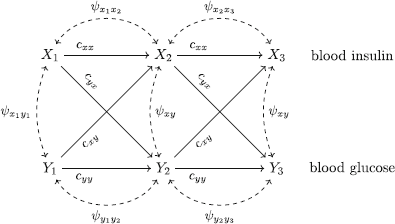


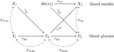


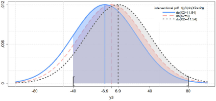


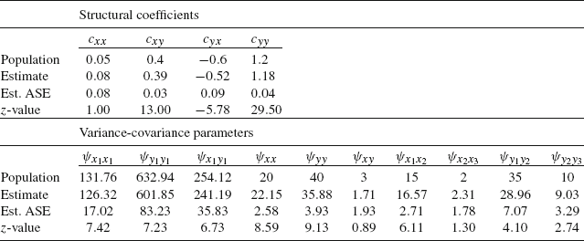

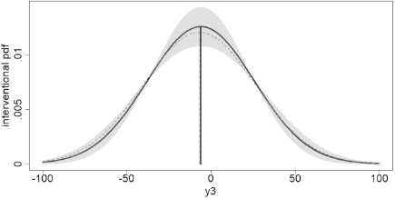


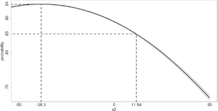


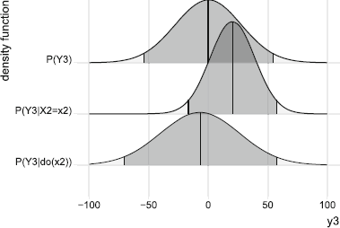


 Open access

