

1. INTRODUCTION
Glaciers in Alaska and adjacent Yukon and British Columbia (~87 000 km2; Kienholz and others, Reference Kienholz2015) are substantial contributors to sea level rise. During the period 2003–09 their rate of mass loss was $ \sim \!\!50\,{\rm Gt} {{\rm \;a}^{ - 1}}$
, ~1/5 of the mass loss of the global glaciers excluding ice sheets (Gardner and others, Reference Gardner2013). The largest mass losses are found in the maritime climates around the Gulf of Alaska (Arendt and others, Reference Arendt, Echelmeyer, Harrison, Lingle and Valentine2002, Reference Arendt2013; Berthier and others, Reference Berthier, Schiefer, Clarke, Menounos and Rémy2010). The mass loss of Alaska's glaciers is expected to continue; for example, Radić and others (Reference Radić2013) project losses between 18 and 45% by the end of the 21st century.
$ \sim \!\!50\,{\rm Gt} {{\rm \;a}^{ - 1}}$
, ~1/5 of the mass loss of the global glaciers excluding ice sheets (Gardner and others, Reference Gardner2013). The largest mass losses are found in the maritime climates around the Gulf of Alaska (Arendt and others, Reference Arendt, Echelmeyer, Harrison, Lingle and Valentine2002, Reference Arendt2013; Berthier and others, Reference Berthier, Schiefer, Clarke, Menounos and Rémy2010). The mass loss of Alaska's glaciers is expected to continue; for example, Radić and others (Reference Radić2013) project losses between 18 and 45% by the end of the 21st century.
Large icefields mantling complex mountainous topographies with strong relief are common in Alaska (e.g. Harding Icefield, Juneau Icefield, Stikine Icefield). Accurate projections of their mass changes are important for assessing the future contribution of Alaska's glaciers to sea level rise. There are two main feedbacks competing in an icefield's response to a warming climate (e.g. Harrison and others, Reference Harrison, Elsberg, Echelmeyer and Krimmel2001; Huss and Farinotti, Reference Huss and Farinotti2012). As outlet glaciers retreat, low-lying, high-ablating parts of the icefield are lost, leading to less negative icefield-wide specific mass balances. This stabilizing (negative) feedback competes with a destabilizing (positive) feedback due to glacier-wide thinning commonly referred to as the Bodvardsson effect (Bodvarsson, Reference Bodvarsson1955) or climate-elevation feedback. As the glacier thins, the surface is exposed to higher temperatures leading to increased melt and further thinning. While for relatively thin mountain glaciers in steep terrain the stabilizing feedback usually dominates, ice caps can fall victim to the destabilizing feedback. For different initial ice thicknesses these feedback mechanisms can then lead to different stable states under the same climate forcing. Juneau Icefield combines the characteristics of an ice cap and mountain glaciers leading us to question which of the two feedbacks will dominate under future climate conditions.
So far, due to the global scope of existing studies, projections of Alaska's icefields have relied on simple scaling methods rather than on physically-based flow modeling to account for glacier front variations (Marzeion and others, Reference Marzeion, Jarosch and Hofer2012; Radić and others, Reference Radić2013). In this study we simulate the recent and future evolution of the Juneau Icefield, the second largest icefield in Alaska, using the open-source Parallel Ice Sheet Model (PISM; Khroulev and the PISM Authors, Reference Khroulev2014) forced by output from the regional Weather Research and Forecasting (WRF) Model. PISM is a hybrid shallow ice, shallow shelf model, which has been extensively applied at a wide range of spatial scales. Applications include the entire Northern hemisphere (Ziemen and others, Reference Ziemen, Rodehacke and Mikolajewicz2014), the Last Glacial Cordilleran Ice Sheet (Seguinot and others, Reference Seguinot, Khroulev, Rogozhina, Stroeven and Zhang2014), the Antarctic and Greenland ice sheets (e.g. Martin and others, Reference Martin2011; Aschwanden and others, Reference Aschwanden, Aðalgeirsdóttir and Khroulev2013), their sub-regions (e.g. Habermann and others, Reference Habermann, Truffer and Maxwell2013), the New Zealand Southern Alps (Golledge and others, Reference Golledge2012) and individual glaciers (van Pelt and others, Reference van Pelt2013). The goal of our work is to project the 21st century evolution of the icefield. We explore the sensitivity of the modeled icefield to model parameters and climatological variables in order to assess the robustness of our results. Finally, we perform a series of model experiments to investigate the stability of the icefield under hypothetical climate stabilization scenarios, and assess the ability to regrow from an ice-free state.
2. PHYSICAL SETTING
The Juneau Icefield is located in the northern Coast Mountains at the border between southeast Alaska and British Columbia (Fig. 1). The icefield presently covers an area of ~3700 km2 and ranges in elevation from sea level at the western and southern margins to 2300 m a.s.l. (Kienholz and others, Reference Kienholz2015). Oriented northwest-southeast, roughly parallel to the coast, the icefield is split into a maritime western part that receives 3–4 m a–1 of precipitation (Pelto and others, Reference Pelto, Kavanaugh and McNeil2013) and a much drier eastern part. Melt occurs across the entire icefield in summer (Ramage and others, Reference Ramage, Isacks and Miller2000), and rainfall and melt are common in the lower parts in winter. All glaciers of the icefield are presently land- or lake-terminating.
Modeling domain including the Juneau Icefield and surrounding glaciers (in total ~4150 km2 based on present-day ice cover; Kienholz and others, Reference Kienholz2015). Colors distinguish individual outlet glaciers. The glaciers south of the Lynn Canal (shown in gray) are excluded in our study.

The largest outlet glacier is Taku Glacier with an area of 735 km2 and a length of 60 km (Kienholz and others, Reference Kienholz2015). Taku Glacier has experienced tidewater glacier cycles (Meier and Post, Reference Meier and Post1987) in past centuries that yielded an advance/retreat pattern largely asynchronous with regional glacier change. Following a rapid tidewater retreat for about a century, in 1850 the glacier began a steady advance that continues today, in sharp contrast to the general retreat and thinning of the other glaciers of the icefield (Motyka and Begét, Reference Motyka and Begét1996; Truffer and others, Reference Truffer, Motyka, Hekkers, Howat and King2009). The glacier has built its own dam by pushing a moraine into the Taku Inlet, protecting itself from marine calving (Motyka and Begét, Reference Motyka and Begét1996; Kuriger and others, Reference Kuriger, Truffer, Motyka and Bucki2006). Therefore the glacier is presently land-terminating. Seismic profiles have revealed local ice thicknesses exceeding 1.4 km and basal troughs reaching down to 600 m below sea level (Nolan and others, Reference Nolan, Echelmeyer, Motyka and Trabant1995).
Llewelyn Glacier is the second largest (450 km2, 37.5 km long), and drains substantial parts of the drier eastern side of the icefield. Mendenhall Glacier (109 km2, 25 km long) close to Juneau is a well-studied glacier that retreated 3 km during the 20th century (Motyka and Echelmeyer, Reference Motyka and Echelmeyer2003). The glacier was historically land-terminating but now ends in a proglacial lake. The calving flux into the lake accounts for only 3–6% of the total net mass loss, but plays an important role in the ongoing retreat. Maximum ice thickness near the terminus is ~70–120 m and reaches ~500–600 m further up-glacier (Motyka and Echelmeyer, Reference Motyka and Echelmeyer2003; Boyce and others, Reference Boyce, Motyka and Truffer2007; Molnia, Reference Molnia2007).
3. PREVIOUS WORK
The Juneau Icefield has been the subject of a variety of glaciological studies. Most of them focused on individual outlet glaciers (e.g. Heusser and Marcus, Reference Heusser and Marcus1964; Pelto and others, Reference Pelto, Kavanaugh and McNeil2013) or included the icefield as part of a much larger domain (e.g. Lawrence, Reference Lawrence1950; Larsen and others, Reference Larsen, Motyka, Arendt, Echelmeyer and Geissler2007; Berthier and others, Reference Berthier, Schiefer, Clarke, Menounos and Rémy2010). Only Ramage and others (Reference Ramage, Isacks and Miller2000) and Melkonian and others (Reference Melkonian, Willis and Pritchard2014) explicitly dealt with the entire Juneau Icefield as such. Here we review relevant previous studies on mass balance and ice velocity, since these data are used for model calibration.
The most prominent study is the long-term monitoring of surface mass balance with focus on Taku and Lemon Creek glaciers (9.5 km2) by the Juneau Icefield Research program, a student training program in operation since 1946 (e.g. Pelto and others, Reference Pelto, Kavanaugh and McNeil2013). Surface mass balance is measured in snow pits in 17 (Taku) and 5 (Lemon Creek) fixed locations between 950 and 1800 m a.s.l. in July and August and adjusted to represent annual balances at the end of the melt season. Ablation stake measurements over a few years revealed net surface mass losses of 12–14 m w.e. a–1 close to the terminus (Pelto and Miller, Reference Pelto and Miller1990; Motyka and Echelmeyer, Reference Motyka and Echelmeyer2003) consistent with losses of 10–14 m w.e. a–1 found close to the terminus of neighboring Mendenhall Glacier between 1998 and 2005 (Boyce and others, Reference Boyce, Motyka and Truffer2007). Glaciological measurements on Mendenhall Glacier indicate an area-averaged mass balance of $ - 0.95 \pm 0.11\,{\rm m} {\rm \;w}. {\rm e}. {{\rm \;a}^{ - 1}}$
from 1948 to 1995 (Motyka and Echelmeyer, Reference Motyka and Echelmeyer2003).
$ - 0.95 \pm 0.11\,{\rm m} {\rm \;w}. {\rm e}. {{\rm \;a}^{ - 1}}$
from 1948 to 1995 (Motyka and Echelmeyer, Reference Motyka and Echelmeyer2003).
Several studies have reported geodetic mass balances over various periods based on sequential DEM comparisons (Table 1). Larsen and others (Reference Larsen, Motyka, Arendt, Echelmeyer and Geissler2007) computed glacier volume changes in southeast Alaska by differencing the Shuttle Radar Topography Mission (SRTM) DEM (acquired in February 2000) with DEMs derived from maps referring to 1948 for Alaska (61% of the Juneau Icefield), and 1982 (17%) or 1987 (22%) for Canada (yielding ~1962 as an area-averaged date). Berthier and others (Reference Berthier, Schiefer, Clarke, Menounos and Rémy2010) subtracted the same early-date DEM from a DEM for 2006 derived from SPOT5 and ASTER images, but most of Taku Glacier and large parts of Llewelyn Glacier were excluded due to data gaps. Melkonian and others (Reference Melkonian, Willis and Pritchard2014) estimated mass change between 2000 and 2009/2013 by applying a weighted linear regression on a pixel-by-pixel basis to elevations from ASTER DEMs stacked with the SRTM DEM.
Previously reported specific mass balance rates $\dot B$
for different periods for the entire Juneau Icefield and Taku Glacier. The Larsen and others (Reference Larsen, Motyka, Arendt, Echelmeyer and Geissler2007) value for Taku is taken from Melkonian and others (Reference Melkonian, Willis and Pritchard2014)
$\dot B$
for different periods for the entire Juneau Icefield and Taku Glacier. The Larsen and others (Reference Larsen, Motyka, Arendt, Echelmeyer and Geissler2007) value for Taku is taken from Melkonian and others (Reference Melkonian, Willis and Pritchard2014)

While there is consensus that the icefield has lost mass over all investigated periods, a less negative rate is found for the period 2000–2009/2013 compared with the earlier periods (Table 1). The difference between the periods can be seen all across the icefield. It must therefore either be caused by different climatic conditions or by systematic differences between the methods. For Taku Glacier the geodetically derived balance rates are generally positive, which is consistent with its current advance, but rates vary between studies. One factor that contributes to the differences between Pelto and others (Reference Pelto, Kavanaugh and McNeil2013) and the other studies are different outlines used for Taku Glacier (Table 1). The glaciological method yields a positive balance for Taku Glacier for the period 1948–2000 and slightly negative mass change rates for more recent periods, although the lack of glaciological measurements in the ablation zone could be a significant source of error (Pelto and others, Reference Pelto, Kavanaugh and McNeil2013).
Melkonian and others (Reference Melkonian, Willis and Pritchard2014) combine ASTER and Japanese ALOS pixel tracking with ERS InSAR-based measurements from various dates between 1995 and 2012 to obtain velocity fields for the icefield. They find maximum speeds of ~1.5 m d–1 along the main trunk of Taku Glacier, with maximum speeds at other outlet glaciers typically ranging from 0.4 to 0.8 m d–1, consistent with maximum speeds of ~0.5–0.6 m d–1 measured by Motyka and Echelmeyer (Reference Motyka and Echelmeyer2003) 1–3 km up-glacier from the terminus of Mendenhall Glacier using GPS between 1997 and 2000.
Using GPS measurements McGee and others (Reference McGee2007) did not detect significant interannual velocity variability in the accumulation area of Taku between 1993 and 2006, but found a slight acceleration along the main trunk at four profiles of 6–7% between 1998/2000 and 2007, an increase too small to be detected by the pixel-tracking results in Melkonian and others (Reference Melkonian, Willis and Pritchard2014). Speeds closer to the terminus of Taku Glacier exhibit pronounced seasonal variability. Truffer and others (Reference Truffer, Motyka, Hekkers, Howat and King2009) found summer speeds ~0.2–0.3 m d–1 higher than the annual average at its terminal kilometer between 2003 and 2005, consistent with observations along the same profiles between 2009 and 2010 made by Melkonian and others (Reference Melkonian, Willis and Pritchard2014).
4. DATA
PISM requires bed elevation and initial ice thickness fields. In addition, we force the model with monthly-mean near-surface (2 m) air temperature and precipitation fields. For model calibration we use the available mass balance data and velocity fields reported in the literature. Additionally we use equilibrium-line altitudes (ELAs) that we derive from late-summer snow lines for individual glaciers of the icefield from satellite data (Section 4.3).
4.1. Ice thickness and bed elevation
Current ice thickness (referring to the year 2000) was derived by M. Huss (personal communication, 2014) using the method of Huss and Farinotti (Reference Huss and Farinotti2012). This approach uses a highly parametrized mass balance to determine the volumetric balance flux along the glacier, which in turn is used to compute spatially distributed ice thicknesses using the isothermal shallow ice approximation applied to the SRTM DEM. Here the method of Huss and Farinotti (Reference Huss and Farinotti2012) is updated to allow ice thicknesses larger than zero along ice divides between individual glaciers. The glacier outlines are taken from Kienholz and others (Reference Kienholz2015). The resulting ice thickness distribution is shown in Figure 2. The average thickness is 270 m and the maximum thickness 1283 m. Total volume is 1120 km3. Given the simplicity of the model, the maximum thickness is in good agreement with the more than 1400 m obtained by Nolan and others (Reference Nolan, Echelmeyer, Motyka and Trabant1995), and calculated thicknesses compare well with observations on Taku Glacier (Huss and Farinotti, Reference Huss and Farinotti2012).
Spatial distribution of ice thickness computed with an updated version of the method by Huss and Farinotti (Reference Huss and Farinotti2012).

We derive the basal topography by subtracting the ice thickness from the SRTM surface topography, and keep it constant. Ice thickness and bed topography grids have the nominal resolution of 30 m of the SRTM DEM.
4.2. Climate data
We use the regional atmospheric model of WRF (Skamarock and others, Reference Skamarock2008) to dynamically downscale near-surface air temperature and precipitation (Figs. 3, 4b) from one of the Coupled Model Intercomparison Project Phase 5 (CMIP5) simulations by the Community Climate System Model 4 (CCSM4; Gent and others, Reference Gent2011). Coarse-scale CMIP5-CCSM4 simulations from the ensemble member Mother of all Runs (MOAR) for the historical period of 1971–2005 and projections for 2006–99 are downscaled with WRF to a 20 km resolution grid covering Alaska and adjacent Canada following the approach by Zhang and others (Reference Zhang, Bhatt, Tangborn and Lingle2007). The projections are forced with the greenhouse gas emission scenario of Representative Concentration Pathway 6.0 (RCP6.0), which is considered a ‘middle-of-the-road’ emission scenario. WRF predicts an increase in near-surface air temperature by 3.6 K averaged over the icefield in summer and by 2.5 K in winter. Changes in precipitation are minor (Table 3).
Mean summer (April–September), annual, and winter (October–March) near-surface air temperatures from the WRF model over the Juneau Icefield and surrounding glaciers (Fig. 1).

Winter (October–March) precipitation fields averaged over the period 1971–2000. (a) 2 km resolution SNAP data based on PRISM. (b) 20 km resolution WRF data. (c) Adjusted WRF data; red lines are isolines of the precipitation correction factor field by which the WRF data are multiplied prior to forcing PISM (Section 6.2). All the data are interpolated to the 300 m ice sheet model grid. Black outline shows the present-day ice extent of the Juneau Icefield.

Winter (October–March), summer (April–September) and annual mean near-surface air temperature and precipitation averaged over the present-day icefield and four periods. The data are based on WRF with the precipitation adjusted as detailed in Section 6.2. The first column refers to the constant climate split-off (S) and regrowth (R) experiments. ΔV and ΔA refer to the volume and area changes relative to the 2010 state of reference run REF. t90 is the number of model years when 90% of the final volume change has occurred, ts is the number of model years when a steady state has been reached according to Eqn (4) and is given relative to 2010 for S-experiments and to the start of the run for the R experiments.

In WRF, the processes that occur at the sub-grid scale are described by various physical parametrizations that are selectable by the user depending on their particular needs. The selection of the most suitable and best-performing parametrizations schemes for a particular region is critical for achieving the best possible performance from WRF. To address this challenge, a series of sensitivity tests to optimize the WRF configuration for application over Alaska and surrounding areas have been carried out (Liu and others, Reference Liu, Krieger and Zhang2013; Zhang and others, Reference Zhang2013).
We bilinearly interpolate the WRF downscaled near-surface temperature and precipitation data from 20 km to the 300 m resolution PISM grid. Air temperatures are corrected for the elevation difference between the WRF topography and the evolving surface elevations of the icefield using a constant lapse rate of $ - 5 {\rm K} {\rm \;k}{{\rm m}^{ - 1}}$
(Abe-Ouchi and others, Reference Abe-Ouchi, Segawa and Saito2007; Ziemen and others, Reference Ziemen, Rodehacke and Mikolajewicz2014). In the following we refer to this dataset as the WRF data.
$ - 5 {\rm K} {\rm \;k}{{\rm m}^{ - 1}}$
(Abe-Ouchi and others, Reference Abe-Ouchi, Segawa and Saito2007; Ziemen and others, Reference Ziemen, Rodehacke and Mikolajewicz2014). In the following we refer to this dataset as the WRF data.
We also tested a high-resolution gridded monthly climate dataset (Fig. 4a) generated by the Scenarios Network for Alaska Planning (SNAP), University of Alaska (retrieved March 2014 from http://www.snap.uaf.edu), which has been created specifically for Alaska. SNAP downscales the Climate Research Unit global reconstruction (Harris and others, Reference Harris, Jones, Osborn and Lister2014) and CMIP5 climate model projections to a higher resolution using the PRISM (Parameter-elevation Relationships on Independent Slopes Model) climate mapping system (Daly and others, Reference Daly, Gibson, Taylor, Johnson and Pasteris2002). PRISM applies a climate/elevation regression for each grid cell. Stations included in the regression are assigned weights based primarily on the physiographic similarity of the station to the grid cell depending on factors such as slope, aspect and coastal proximity.
The SNAP data have a high nominal spatial resolution of 2 km, but the very few weather stations available in the study area are concentrated at lower elevations, leaving PRISM relatively uninformed at higher elevations. Hence PRISM precipitation fields largely depend on altitude (Fig. 4a), resulting in a precipitation maximum on the highest parts of the icefield. This conflicts with our expectations for orographic effects of large mountain chains (e.g. Roe, Reference Roe2003) which suggest a precipitation maximum on western and southern flanks of the icefield. A precipitation maximum on the flanks is also necessary for our mass balance modeling to match the existing mass balance measurements (Section 6.2).
The WRF data, in contrast, have a resolution of 20 km, but WRF directly models the atmosphere dynamics and places the precipitation maximum in the southwestern part of the icefield. The WRF and SNAP precipitation data differ both in total amounts and spatial distribution. WRF's total winter (October–March) precipitation is 2.2 m averaged over the entire icefield for 1971–2000, 0.40 m less than the SNAP data for the same period. Comparing each grid cell's winter precipitation, the RMS difference between the SNAP and WRF datasets is 0.74 m, indicating substantial differences in spatial pattern. The icefield average near-surface air temperature is higher in the SNAP dataset by 5.7 K in summer (April–September) and 5.8 K in winter (October–March). The RMS is 5.8 K in summer and 6.1 K in winter. The differences are smaller in the low-lying areas (<50 m a.s.l.), where weather stations contribute to PRISM (and thus the SNAP dataset), with summer temperatures 2.9 K, and winter temperatures 0.9 K higher in the SNAP dataset.
4.3. Equilibrium line altitudes
We map snowlines for individual glaciers of the icefield from nine Landsat 5 Thematic Mapper (TM) satellite scenes as well as three Landsat 7 Enhanced Thematic Mapper (ETM+) and four Landsat 8 Operational Land Imager (OLI) scenes, covering the period 1996–2014. We aim at annual (end-of-summer) snowlines but due to frequent cloud cover we analyze all cloud-free images from August to September. In case several snowlines are available for the same glacier and year, we retain the highest. We determined each snowline's characteristic altitude by calculating the median of the SRTM altitudes within 30 m of the snowline. Since we assume superimposed ice to be negligible, the snow line altitudes are equivalent to ELAs (Cogley and others, Reference Cogley2011), thus allowing us to compare them with modeled ELAs for model calibration. The method of deriving the snowlines is detailed in Appendix A.
5. MODEL DESCRIPTION AND APPLICATION
5.1. The Parallel Ice Sheet Model
The Parallel Ice Sheet Model (PISM) includes a hybrid stress balance model (Bueler and Brown, Reference Bueler and Brown2009; Aschwanden and others, Reference Aschwanden, Bueler, Khroulev and Blatter2012) combining the Shallow Ice Approximation (Hutter, Reference Hutter1983) for vertical deformation and the Shallow Shelf Approximation (Morland, Reference Morland, van der Veen and Oerlemans1987) for longitudinal stretching. The ice rheology is described using Glen's flow law
 $$D = E A \vert \tau { \vert ^{n - 1}}\tau, $$
where D is the strain rate tensor, E is the flow enhancement factor, a tuning parameter used to account for unresolved aspects of the ice flow, A is the rate factor, τ is the deviatoric stress tensor and n = 3 is the flow law exponent. The whole Juneau Icefield is assumed to be temperate; consequently we run PISM in an isothermal configuration and use a constant rate factor of $A = 4.5293 \times {10^{ - 24}} P{a^{ - 3}} {s^{ - 1}}$
, the result of the Paterson and Budd (Reference Paterson and Budd1982) rate factor equation for ice at the melting point. We refrain from lumping A and E into one single parameter in Eqn (1) to facilitate the interpretation of the corresponding sensitivity experiments.
$A = 4.5293 \times {10^{ - 24}} P{a^{ - 3}} {s^{ - 1}}$
, the result of the Paterson and Budd (Reference Paterson and Budd1982) rate factor equation for ice at the melting point. We refrain from lumping A and E into one single parameter in Eqn (1) to facilitate the interpretation of the corresponding sensitivity experiments.
We parametrize basal sliding using a power law with a quadratic dependence of the basal velocity ${\vec u_{\rm b}}$
on the basal stress
${\vec u_{\rm b}}$
on the basal stress ${\vec \tau _{\rm b}}$
,
${\vec \tau _{\rm b}}$
,
 $${\vec u_{\rm b}} = - {u_{\rm c}}\displaystyle{{ \vert {{\vec \tau} _{\rm b}} \vert {{\vec \tau} _{\rm b}}} \over { \vert {\tau _{\rm c}}{ \vert ^2}}},$$
where τ
c (units of stress) and u
c (units of velocity) are two tuning parameters representing only one degree of freedom. Using two parameters instead of one simplifies the interpretation of the sliding law. We set ${u_{\rm c}} = 500\,{\rm m} {{\rm a}^{ - 1}}$
, while τ
c, a pseudo-yield-stress, is part of the calibration procedure (Section 6.1).
${u_{\rm c}} = 500\,{\rm m} {{\rm a}^{ - 1}}$
, while τ
c, a pseudo-yield-stress, is part of the calibration procedure (Section 6.1).
Surface mass balance is computed as the difference between accumulation and ablation. Precipitation is split into solid and liquid fractions using a linear transition between − 10 and +7°C monthly mean surface air temperature based on observations analyzed by (Marsiat, Reference Marsiat1994). The large range is explained by the use of monthly mean data rather than instantaneous temperatures. The solid fraction of precipitation is treated as snow accumulation and converted to ice at the end of each mass balance year (end of September). The liquid fraction is discarded as runoff. Ablation is computed from monthly near-surface air temperature using a positive degree day (PDD) scheme (Hock, Reference Hock2003). Temperatures within each month are described by a normal distribution and the PDD integral is evaluated analytically using the error function (Calov and Greve, Reference Calov and Greve2005). Following Ziemen and others (Reference Ziemen, Rodehacke and Mikolajewicz2014) we implement this approach by providing PISM with monthly maps of temperature mean and standard deviation computed from the hourly WRF output.
The model is set up on Alaska Albers equal area coordinates with a horizontal resolution of 300 m. Interpolation from the SRTM grid to the PISM grid is done conservatively. The modeling domain covers the Juneau Icefield and surrounding unconnected glaciers (Fig. 1). For this domain, the adaptive time stepping yields time steps of ~8 h. Each run took ~36 h on 64 CPUs including spinup. All simulations used PISM version 0.6. Due to the limited spatial and temporal scale of the experiments we did not model isostatic rebound.
5.2. Model spinup
We perform a multi-stage spinup to avoid spurious mass changes resulting from coupling shocks at the start of the experiments. These would interfere with the tuning and validation. As a starting point for the spinup, we compute an initial ice thickness field by projecting the year 2000 ice thickness field (Section 4.1) back in time by 60 a to 1940 using the thickness change rates from Larsen and others (Reference Larsen, Motyka, Arendt, Echelmeyer and Geissler2007). As climate forcing we use the 1971–2000 climate data, because this is the first 30 a interval for which we have downscaled the climate data available. We choose 30 years to average out short-term variability.
During the spinup, we nudge the model to the 1940 ice thickness using Newtonian relaxation (e.g. Jeuken and others, Reference Jeuken, Siegmund, Heijboer, Feichter and Bengtsson1996). After each time step the deviation of modeled ice thickness from the targeted ice thickness ΔH of each grid cell is scaled by a relaxation factor γ, and that value is subtracted from the following time step's surface mass balance. For example, for γ = 0.1 a−1 and a thickness deviation of ΔH = 1 m, the surface mass balance rate computed with the PDD scheme is reduced by $\gamma \Delta H = 0.1 \,{\rm m}{{\rm \;a}^{ - 1}}$
.
$\gamma \Delta H = 0.1 \,{\rm m}{{\rm \;a}^{ - 1}}$
.
We run the model for 90 years repeating the 1971–2000 climate data three times. For the first 60 years we employ a relaxation constant $\gamma = 0.1 \,{{\rm a}^{ - 1}}$
. This allows the icefield to evolve into a state that is consistent with the model physics, while keeping the surface elevations very close to the reconstructed 1940 state. For the remaining 30 years we decrease the constant to
$\gamma = 0.1 \,{{\rm a}^{ - 1}}$
. This allows the icefield to evolve into a state that is consistent with the model physics, while keeping the surface elevations very close to the reconstructed 1940 state. For the remaining 30 years we decrease the constant to $0.01 \,{{\rm a}^{ - 1}}$
to arrive at the 1971 initial thickness field. The reduction of γ in the last cycle allows the icefield to evolve almost freely to avoid a coupling shock when starting the experiments. The short spin-up is possible because the ice flow does not depend on ice temperature in our setup.
$0.01 \,{{\rm a}^{ - 1}}$
to arrive at the 1971 initial thickness field. The reduction of γ in the last cycle allows the icefield to evolve almost freely to avoid a coupling shock when starting the experiments. The short spin-up is possible because the ice flow does not depend on ice temperature in our setup.
6. CALIBRATION
The model is calibrated by performing hindcasts for the period 1971–2010 and comparing the hindcasts with four sets of observations: surface speeds (Melkonian and others, Reference Melkonian, Willis and Pritchard2014), the mean 1946–86 surface mass balance gradient (Pelto and Miller, Reference Pelto and Miller1990), our satellite-derived transient ELAs for individual outlet glaciers and multi-year geodetic mass change (Table 1). Since the WRF data are produced by a free running climate model, we cannot expect individual model years or even decadal means to line up with corresponding observations, and therefore only compare long-term averages. The model run using the calibrated model parameters is referred to as reference run (REF) in the following.
6.1. Ice flow
To calibrate the two ice dynamics parameters, E (Eqn (1)) and τ
c (Eqn (2)), we run PISM's surface relaxation scheme with a relaxation constant of $0.1 \,{\rm m}{{\rm \;a}^{ - 1}}$
. This isolates the effect of the flow parameters from the effects of the surface mass balance and the surface evolution. At the same time, the surface can slightly adjust to the flow, thereby smoothing out local inconsistencies between prescribed surface and flow physics. We find E = 1 and τ
c = 0.5 MPa provide reasonable agreement between the modeled and observed ice velocities (RMS difference of
$0.1 \,{\rm m}{{\rm \;a}^{ - 1}}$
. This isolates the effect of the flow parameters from the effects of the surface mass balance and the surface evolution. At the same time, the surface can slightly adjust to the flow, thereby smoothing out local inconsistencies between prescribed surface and flow physics. We find E = 1 and τ
c = 0.5 MPa provide reasonable agreement between the modeled and observed ice velocities (RMS difference of $69 \,{\rm m}{{\rm \;a}^{ - 1}}$
; Fig. 5).
$69 \,{\rm m}{{\rm \;a}^{ - 1}}$
; Fig. 5).
(a) Measured surface speed (Melkonian and others, Reference Melkonian, Willis and Pritchard2014), (b) modeled surface speed and (c) modeled basal sliding speed.

6.2. Surface mass balance
In a first step we calibrate the surface mass balance model by adjusting the PDD factors for ice and snow to match the observed mass balance profile over Taku Glacier (Fig. 6).
Surface mass balance vs surface elevation for Taku Glacier. The black curve indicates the average profile derived from measurements between 1948 and 1986 (Pelto and Miller, Reference Pelto and Miller1990). Green dots mark modeled surface mass balances of all Taku Glacier grid cells averaged over the period 1971–2000.

Using the 2 km resolution SNAP dataset (Section 4.2; Fig. 4a), it was impossible to reproduce the observed mass balance profile, while keeping PDD factors within reasonable ranges. While the SNAP data show high winter precipitation, especially at high altitudes (Fig. 4a), it also shows relatively high air temperatures over the icefield (Supplementary Figure S1), yielding a too negative mass balance at all elevations, even for unrealistically low PDD factors (Supplementary Figure S2a). We investigated possible systematic temperature biases. To increase the surface mass balance, we decreased the temperature by 2.5 K uniformly in the whole domain. With this temperature field, a reasonable fit to the Pelto and Miller (Reference Pelto and Miller1990) mass balance profile could only be obtained for a snow PDD factor of $0.5{\kern 1pt} \,{\rm mm}\,{{\rm K}^{ - 1}}{\kern 1pt} {{\rm d}^{ - 1}}$
(Supplementary Figure S2b) and an ice PDD factor of
$0.5{\kern 1pt} \,{\rm mm}\,{{\rm K}^{ - 1}}{\kern 1pt} {{\rm d}^{ - 1}}$
(Supplementary Figure S2b) and an ice PDD factor of $14{\kern 1pt} \,{\rm mm}\,{{\rm K}^{ - 1}}{\kern 1pt} {{\rm d}^{ - 1}}$
. However, the PDD factor for snow is unrealistically low and indicates that the high altitudes are still too warm. We therefore decreased the air temperatures even further by a total of 5 K and found best agreement with the observed mass balance profile using
$14{\kern 1pt} \,{\rm mm}\,{{\rm K}^{ - 1}}{\kern 1pt} {{\rm d}^{ - 1}}$
. However, the PDD factor for snow is unrealistically low and indicates that the high altitudes are still too warm. We therefore decreased the air temperatures even further by a total of 5 K and found best agreement with the observed mass balance profile using ${\rm PD}{{\rm D}_{{\rm snow}}} = 2\,{\rm mm}\,{{\rm K}^{ - 1}}{\kern 1pt} {{\rm d}^{ - 1}}$
and
${\rm PD}{{\rm D}_{{\rm snow}}} = 2\,{\rm mm}\,{{\rm K}^{ - 1}}{\kern 1pt} {{\rm d}^{ - 1}}$
and ${\rm PD}{{\rm D}_{{\rm ice}}} = 14\,{\rm mm}\,{{\rm K}^{ - 1}}{\kern 1pt} {{\rm d}^{ - 1}}$
(Supplementary Figure S2b). These factors are too far apart from each other to be plausible (Hock, Reference Hock2003). They indicate a too small temperature difference between accumulation and ablation areas. Overall, this provides further circumstantial evidence that the spatial distribution of air temperature and precipitation over the icefield is not realistic in the SNAP data.
${\rm PD}{{\rm D}_{{\rm ice}}} = 14\,{\rm mm}\,{{\rm K}^{ - 1}}{\kern 1pt} {{\rm d}^{ - 1}}$
(Supplementary Figure S2b). These factors are too far apart from each other to be plausible (Hock, Reference Hock2003). They indicate a too small temperature difference between accumulation and ablation areas. Overall, this provides further circumstantial evidence that the spatial distribution of air temperature and precipitation over the icefield is not realistic in the SNAP data.
In contrast, we are able to obtain a good fit to the observed mass balance profile by using the dynamically downscaled WRF data (Section 4.2). The fit to the Pelto and Miller (Reference Pelto and Miller1990) mass balance profile is best for snow and ice factors of 4 and 10 mm w.e. a–1 respectively, consistent with the range of values typically found in the literature (Hock, Reference Hock2003). Observed ELAs range between ~800 m a.s.l. in the western part and ~1600 m a.s.l. in the eastern part (Supplementary Figure S3). Compared with the observations, modeled ELAs are considerably higher in the western part and lower in the eastern part (Fig. 7b). We attribute this discrepancy to the WRF model not resolving the pronounced precipitation gradient across the icefield in the west-east direction, which is caused by orographic effects on a spatial scale too small to be resolved by the climate model (Fig. 4b).
Modeled annual ELAs for the period 1990–2019 vs observed ELAs for the period 1996–2014 for individual glaciers of the Juneau Icefield. The time window for the model data is chosen as 30 years, centered on the observation period. Dark filled circles show the median of all available annual modeled and observed values for each glacier. Large circles mark glaciers >100 km2. Small dots connected by lines mark the ELAs for each individual year (blue: modeled; green: observed). Also shown are 1 : 1-line (light gray) and linear fit of the medians (dark line). (a) Model run REF with precipitation adjustment to account for systematic bias (Section 6.2). (b) Model run NOGRAD using the WRF data without precipitation adjustment.

We account for this apparent systematic bias by adjusting the precipitation fields so that precipitation near the coast is increased, while it is decreased on the eastern side of the icefield. Similar to Aðalgeirsdóttir and others (Reference Aðalgeirsdóttir, Gudmundsson and Björnsson2003), we fit a plane, $z = a x + b y + c$
with a = 8.41 × 10⁻³, b = 9.36 × 10⁻³ and c = −58 616 m through the observed ELAs, where x and y are the coordinates in Alaska Albers projection. From this field z, we derive a precipitation correction factor ζ for each grid cell:
$z = a x + b y + c$
with a = 8.41 × 10⁻³, b = 9.36 × 10⁻³ and c = −58 616 m through the observed ELAs, where x and y are the coordinates in Alaska Albers projection. From this field z, we derive a precipitation correction factor ζ for each grid cell:
 $$\zeta = \alpha (a x + b y + \beta ) + 1.$$
This parametrization maintains the direction of the gradient, but adjusts the slope and the offset to obtain a field with values decreasing from ~1.5 near the western margin to 0.5 near the eastern margin of the icefield (red lines in Fig. 4c). The offset $\beta = 1200 \,{\rm m} - c = - 59816\,{\rm m}$
was chosen to roughly conserve the total amount of winter precipitation over the present-day icefield, and to provide a smooth gradient across the whole ice-covered area. The slope factor α is determined from tuning. The optimized value is
$\beta = 1200 \,{\rm m} - c = - 59816\,{\rm m}$
was chosen to roughly conserve the total amount of winter precipitation over the present-day icefield, and to provide a smooth gradient across the whole ice-covered area. The slope factor α is determined from tuning. The optimized value is $\alpha = - 1.5 \times {10^{ - 3}} {{\rm m}^{ - 1}}$
. The line for ζ = 1, where precipitation stays unaltered, is independent of α. To maintain a minimum precipitation in the northeast, all values of ζ below 0.1 are set to 0.1. Multiplication with this field results in a new adjusted precipitation field (Fig. 4c) used as input for PISM. Forcing the model with this precipitation field yields ELAs that correlate well with observed ELAs (Fig. 7a) while maintaining a good fit to the observed mass balance profile on Taku Glacier (Fig. 6).
$\alpha = - 1.5 \times {10^{ - 3}} {{\rm m}^{ - 1}}$
. The line for ζ = 1, where precipitation stays unaltered, is independent of α. To maintain a minimum precipitation in the northeast, all values of ζ below 0.1 are set to 0.1. Multiplication with this field results in a new adjusted precipitation field (Fig. 4c) used as input for PISM. Forcing the model with this precipitation field yields ELAs that correlate well with observed ELAs (Fig. 7a) while maintaining a good fit to the observed mass balance profile on Taku Glacier (Fig. 6).
The modeled ELAs are on average ~100 m above the observed ones possibly because the observed ELAs represent snapshots in late summer, but not necessarily the maximum level during the season. They therefore provide a lower estimate of the annual ELAs. Lowering the modeled ELAs by reducing the degree-day factors (sensitivity experiment SMELT↓, Section 7.2) leads to a better fit (Supplementary Figure S4), but also increases the icefield's total mass balance for the period 1971–2010, which is inconsistent with observations (Table 1). With the slightly elevated ELAs, the modeled icefield-wide mass balance rate for the period 1971–2010 is consistent with the observed glacier-wide balances found in previous studies. The spatial pattern of the results during the reference period largely agrees with the observations, (Supplementary Figure S5) although the model shows unrealistic growth on Gilkey Glacier. Due to the large discrepancies we put less emphasis on matching the exact geodetic mass balance observations, but aim to reproduce the large-scale spatial patterns of change with negative balance rates for the calibration period within the observed range of −0.62 to $ - 0.13{\kern 1pt} \,{\rm m\ w}.{\kern 1pt} {\rm e}.{{\rm \;a}^{ - 1}}$
(Table 1) for the entire icefield, while maintaining a positive mass balance for Taku Glacier (Supplementary Figure S5).
$ - 0.13{\kern 1pt} \,{\rm m\ w}.{\kern 1pt} {\rm e}.{{\rm \;a}^{ - 1}}$
(Table 1) for the entire icefield, while maintaining a positive mass balance for Taku Glacier (Supplementary Figure S5).
7. RESULTS
7.1. Icefield evolution 1971–2099
The ice volume evolution of the reference run REF for the period 1971–2099 is shown in Figure 8 (black curve). During the calibration period 1971–2010, ice volume increases slightly by 2% between 1971 and 1996, which is followed by a pronounced decrease, leading to an overall volume loss for 1971–2010 of $62{\kern 1pt} \,{\rm k}{{\rm m}^3}$
(5%). The corresponding specific balance rate of
$62{\kern 1pt} \,{\rm k}{{\rm m}^3}$
(5%). The corresponding specific balance rate of $ - 0.33{\kern 1pt} \,{\rm m}\,{\rm \; w}.{\kern 1pt} {\rm e}.{{\rm \;a}^{ - 1}}$
falls within the range of reported multi-decadal estimates (Table 1). The decrease in ice volume following 1996 is consistent with simultaneous pronounced summer warming (Fig. 3). Mass gains are modeled on Taku and Gilkey Glacier (Supplementary Figure S5).
$ - 0.33{\kern 1pt} \,{\rm m}\,{\rm \; w}.{\kern 1pt} {\rm e}.{{\rm \;a}^{ - 1}}$
falls within the range of reported multi-decadal estimates (Table 1). The decrease in ice volume following 1996 is consistent with simultaneous pronounced summer warming (Fig. 3). Mass gains are modeled on Taku and Gilkey Glacier (Supplementary Figure S5).
Modeled evolution of annual ice volumes over the period 1971–2100 for the reference run and the sensitivity experiments (Table 2). The legend is sorted by final ice volume. Experiments in which the same parameter is varied share the same color.

From 2010 to 2040 volume loss rates are almost linear and all outlet glaciers except for Gilkey and Taku are shrinking. Volume loss rates accelerate and by 2070, most outlet glaciers have negative glacier-wide balances. By the end of 2099 the entire icefield has lost 63% of its volume and 62% of its area compared with 2010. Most of the outlet glaciers have retreated substantially and the northern parts of the icefield have disappeared (Fig. 9d). In contrast Taku and Gilkey Glacier have thinned substantially, but show only a slight retreat. The surface mass balance averaged over the period 2070–99 is negative everywhere except for the high-elevation areas of Taku and Llewelyn glaciers. Despite their positive surface mass balances, these regions are losing mass by dynamic thinning.
Modeled ice thicknesses in year (a) 2011, (b) 2041, (c) 2071 and (d) 2099.

7.2. Uncertainty and sensitivity analysis
Uncertainties in projections arise from inaccuracies in input data, inadequacies in model physics and the calibration procedure. Error propagation cannot be applied in this study because the validity of inherent assumptions, such as normality or independence of parameters, cannot be tested. Therefore, we evaluate uncertainties by assessing the sensitivity of projected volume changes to the choice of model parameters: the flow enhancement factor E (Eqn (1)), the yield stress τ c (Eqn (2)), the PDD factors for snow and ice, the slope factor α (Eqn (3)), the initial ice thickness and the grid resolution. For most parameters or variables we analyze the effects of a positive and negative change relative to the reference run REF and leave all other parameters unaltered (Table 2). For the ice thickness experiments, the initial ice thickness field (Section 5.2) is multiplied by a constant factor prior to spin-up, and basal topography is adjusted accordingly, leaving the surface elevations unchanged.
Sensitivity experiments including varied parameters, and key results. f
α
is a factor by which α is multiplied to vary the strength of the precipitation adjustment (Eqn (3)), PDDs and PDDi are the positive degree-day factors for snow and ice, respectively, E and τ
c are flow parameters (Eqns (1) and (2)), f
thk is the factor by which the initial ice thickness field is multiplied. Displayed results are icefield-wide specific surface mass balance rate $\dot B$
, volume change ΔV and area change ΔA for the calibration period 1971–2010 and the projection period 2011–99, and 2099 volume relative to the volume of Ref in 2099 V
rel. Parameters varied in each experiment are in bold. Modeled
$\dot B$
, volume change ΔV and area change ΔA for the calibration period 1971–2010 and the projection period 2011–99, and 2099 volume relative to the volume of Ref in 2099 V
rel. Parameters varied in each experiment are in bold. Modeled $\dot B$
consistent with the observed range (–0.62 to –0.13 m w.e. a–1, Table 1) are in italic.
$\dot B$
consistent with the observed range (–0.62 to –0.13 m w.e. a–1, Table 1) are in italic.

Sensitivity experiments are carried out by running each experiment first through the spin-up and then from 1971 to 2099. Consequently, each experiment has a different ice volume at the beginning of the prognostic simulation. This procedure avoids shocks in the model that would result from sudden parameter changes.
Initial ice volumes in 1971 are within ~10% of the REF volume and most experiments show similar patterns of volume change throughout the simulation period, 1971–2099. Experiments that start at an elevated ice volume in 1971 also stay at an elevated volume throughout the experiment (and vice versa). In most cases there are no substantial deviations in the pattern of changes from those of the reference run. For those experiments where there are significant deviations, we list them in the following and show characteristic examples in Figure 10. Section 8.3 includes a discussion of the results.
Ice thickness differences in 2099 for two sensitivity experiments. (a) NOGRAD−REF. (b) RES ↓ −REF. Note the different color scales.

Experiments that strongly deviate from the volume loss rate in REF are those where we changed the ice thickness. Experiment THICK starts with 18% greater ice volume, but due to a substantially larger volume loss rate, the ice volume by 2099 is similar to that of REF. The increased ice thickness causes an acceleration in ice flow and therefore increased transport of ice to lower, high-ablating elevations. In addition the decreased basal topography allows for more glacier area at lower elevations. Despite a considerably lower initial ice volume (18%) than REF, the experiment THIN also drops to a similar 2099 ice volume as REF. The year 2099 volumes of THIN and THICK are within 2% of REF.
Varying the enhancement factor by a factor of 1.5 (SLOW, FAST) shows only modest impact on the evolution of the ice volume. The differences in the 2100 ice thickness resulting from variations in the flow parameters are spatially very homogeneous, and do not show any substantial differences between outlet glaciers and the interior of the icefield (not shown).
Varying the PDD factor for ice by ±1 mm K–1 d–1 (IMELT↓, IMELT↑) has little effect on the ice volume evolution. In contrast, varying the snow PDD factor by the same amount strongly affects the ice volume evolution (SMELT↓, SMELT↑).
Compared with REF, running the model without the precipitation adjustment (NOGRAD) results in a 55% higher ice volume in 2100 and yields considerably greater ice thicknesses and ice extent in the north-eastern side of the icefield, in particular on Llewelyn Glacier, and thinner ice in the south. As a result the icefield is shifted to the northeast (dipole pattern in Fig. 10a). In contrast, a higher gradient (GRAD↑) in the precipitation field causes a westward migration (not shown).
Decreasing the model grid resolution from 300 to 600 m (RES↓) leads to an increase in ice thickness, especially on narrow outlet glaciers (Fig. 10b). As outlet glaciers in narrow valleys are less well resolved, the ice slows down leading to dynamic thickening at higher surface elevations, which in turn increases the icefield-wide mass balance. The unrealistically strong growth of Gilkey Glacier may also result from more inflow from the interior of the icefield. The 600 m resolution grid does not properly resolve the mountain ranges separating the glacier from the interior of the icefield and more ice can spill over into the valley. This is consistent with a band of no or negative thickness change around Gilkey Glacier (Fig. 10b). Similar effects may explain the greater ice thicknesses on Mendenhall Glacier.
Eight of the sensitivity experiments yield a mean mass balance rate over the calibration period 1971–2010 that is within the geodetically derived rates of −0.62 to $ - 0.13\,{\kern 1pt} {\rm m}\,{\rm \;w}.{\kern 1pt} {\rm e}.{{\rm \;a}^{ - 1}}$
(Table 2). These experiments also show reasonable agreement between modeled and observed ELAs, Taku Glacier's mass balance profile (Supplementary Figure S4) and observed patterns of mass change during the calibration period (Supplementary Figure S5). Hence, we consider these projections equally plausible as the reference run. Volume changes from 2010 to 2099 for these runs range between 58 and 68%, and area changes range between 57 and 63%.
$ - 0.13\,{\kern 1pt} {\rm m}\,{\rm \;w}.{\kern 1pt} {\rm e}.{{\rm \;a}^{ - 1}}$
(Table 2). These experiments also show reasonable agreement between modeled and observed ELAs, Taku Glacier's mass balance profile (Supplementary Figure S4) and observed patterns of mass change during the calibration period (Supplementary Figure S5). Hence, we consider these projections equally plausible as the reference run. Volume changes from 2010 to 2099 for these runs range between 58 and 68%, and area changes range between 57 and 63%.
7.3. Constant-climate split-off experiments
All projections above are based on the RCP6.0 scenario and show continuous volume losses throughout the 21st century, suggesting a likely disappearance of the icefield, if the temperature and precipitation trends were to continue. Here we investigate whether or not the icefield is able to survive and reach a new steady state, if air temperature and precipitation stabilize earlier in this century. We perform four constant-climate split-off experiments. In the first experiment PISM is forced repeatedly with the climate of the calibration period (1971–2010). Three additional experiments start in 1971 with the transient climate scenario but the model is forced repeatedly with the 2011–40, 2041–70 and 2071–99 time series beyond the years 2040, 2070 and 2099 respectively. We refer to these four experiments as S2010, S2040, S2070 and S2099 in the following. Simulations run for 1500 years or until a steady state is reached, whichever occurs first. We define that a steady state has been reached at time t, if the criterion
 $$\displaystyle{{\sum\nolimits_{i,j} { \vert {H_{i,j}}(t) - {H_{i,j}}(t - \Delta t) \vert}} \over {\Delta t\sum\nolimits_{i,j} {1/2({H_{i,j}}(t) + {H_{i,j}}(t - \Delta t))}}} \lt \displaystyle{{1\%} \over {100 {\rm a}}},$$
is fulfilled, where H i,j is ice thickness at grid point (i,j) and t and t − Δt are the end times of two consecutive climate forcing cycles. This criterion is different than requiring the volume change rate to be lower than 1% per century. The use of the absolute value of the local differences prevents a steady state from being inferred when opposing mass trends in different areas of the icefield cancel.
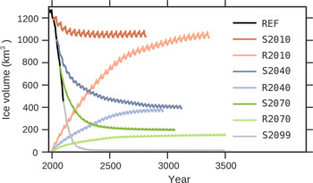
Key results and the statistics on temperature and precipitation for the four stabilization scenarios are given in Table 3 and Figures 11 and 12. The experiments are forced with segments of the transient climate, and therefore experience cycles of climate warming that are followed by step-like cooling at the beginning of the following cycle. This leads to cyclic growth and retreat of the icefield during the split-off experiments (Fig. 11).
Modeled annual ice volumes for the constant climate split-off (S) and regrowth (R) experiments. Experiments with the same climate share shades of the same color. S-experiments start with present-day ice volumes, while R-experiments start from an ice-free state at nominal year 2000. Except for REF, the legend is sorted by final ice volume. Runs end either when a steady state is reached (Table 3) or in year 3500, whichever comes first.
Modeled ice thickness (m) at the end of constant-climate split-off experiments (a) S2010, (b) S2040, (c) S2070 and (d) of the regrowth experiment R2070.

The experiment forced with the climate from the calibration period (S2010) shows a stabilization of the icefield volume at slightly above 1000 km3, corresponding to a loss of 14% of the ice volume in 2010. Substantial area losses and glacier retreats are projected, in particular, in the northern part of the icefield but also in the east (Fig. 12a). Gilkey and Taku Glacier are projected to advance.
Experiments S2040 and S2070 show substantial volume and area losses, but the icefield survives in the higher reaches of the mountains, reaching a steady state after 1110 and 1050 years respectively. Most of the volume changes occur much earlier. While it takes S2040 460 years to reach 90% of the volume change, S2070 passes that mark after 280 years. The earlier stabilization in S2070 compared with S2040 occurs because the warmer climate causes an expansion of the ablation areas, which results in a more rapid retreat to higher elevations than in the cooler scenario. Assuming the 2071–99 climate remains constant (S2099), the icefield's volume rapidly declines to 4% of its 2010 volume by 2220, and continues to decrease thereafter, but at a greatly reduced rate, with some ice still remaining after 1500 years.
7.4. Regrowth experiments
To further investigate the multi-stability of the icefield, and to shed light on the potential of the Juneau Icefield for glaciation, we also perform regrowth experiments (R2010, R2040, R2070). Experiments start from zero ice thickness and are run with repeated climate segments of the corresponding split-off experiments. A regrowth experiment with the 2071–99 climate is not performed since this climate leads to the destruction of the icefield in the split-off experiment S2099. To simplify interpretation we set all experiment start times to year 2000. In all the three experiments, the icefield nucleates in the high-elevation areas and subsequently fills lower-elevation valleys. R2010 and R2040 reach states that are very similar to S2010 and S2040 respectively, and would converge further for longer experiment duration. In contrast, R2070 grows to a volume 24% smaller than S2070 since it is not able to re-occupy the deep troughs of Taku and Llewelyn valleys (Figs. 11, 12c, d).
8. Discussion
8.1. Icefield evolution
Our reference run, forced by the RCP6.0 emission scenario, indicates substantial volume losses by 2100 (64% relative to 2010). Volume losses range from 58 to 68% for the eight sensitivity experiments that are within observational uncertainty in the calibration period. This exceeds the range of 18–45% projected for all Alaskan glaciers with 14 general circulation models for RCP4.5 and RCP8.5 scenarios by Radić and others (Reference Radić2013).
Under the 2071–2100 climate (S2099) the icefield almost completely disappears. All other climate split-off experiments indicate substantial volume losses but the icefield is able to reach a new steady state by retreating to higher elevations.
Assuming the present climate conditions, the icefield stabilizes at a volume only 14% lower than the 2010 volume, which is in sharp contrast to the low-elevation Yakutat Icefield (342 km2, ~200 km to the northwest). When forced by projections from the same climate model and emission scenario, Yakutat Icefield collapses completely by 2070 and, under the present climate conditions, by 2110 (Truessel and others, Reference Truessel2015). The different behavior is due to distinctly different topographies. The Juneau Icefield is able to reach a new steady state due to significantly higher maximum elevations where the glaciers can retreat (2000 vs 650 m a.s.l.). Thus, in Yakutat Icefield, the destabilizing mass balance – elevation feedback dominates, while in Juneau Icefield the stabilizing feedback prevails.
Overall, our experiments show that the icefield is not simply bi-stable as climate warms, but exhibits a variety of possible retreat states. These retreat states are largely controlled by the climate and are independent of the initial geometry. In two out of three scenarios, the icefield state obtained by starting from the present-day geometry is practically identical to the state obtained by starting from a completely removed icefield. Only in one of the three climate forcings (R2070), some parts of the icefield cannot be regrown due to the elevation-mass balance feedback.
The survival of parts of the icefield under warming scenarios and the regrowth from an ice-free state are possible because of the complex topography of the Juneau Icefield. There are a multitude of narrow valleys and several regions where the glaciers can retreat up into high-elevation mountains, which allows them to maintain areas with positive surface mass balance even under the applied warming scenarios. However, even under the fairly moderate S2040 climate scenario, the icefield loses two-thirds of its volume and more than half of its area in the long-term. This shows that, independent of the exact climate trajectory, we have to expect large glacier mass changes in this region.
8.2. Model performance and input data
Good agreement with surface mass balance observations was not achieved using unaltered SNAP and WRF climate data directly, although both datasets were specifically designed for Alaska. The 2 km SNAP data product is based on extrapolation of weather station data, but largely relies on elevation dependency due to sparsity of weather stations in the region. Hence it cannot resolve the intricate precipitation patterns in this region. WRF simulates the dynamics of the atmosphere, and thus more adequately captures spatial patterns other than elevation dependence. However, the grid spacing is too coarse to fully resolve the slope precipitation on the steep flanks of the Juneau Icefield. It therefore cannot capture the strong gradient in precipitation from the coast to the interior.
Only by substantially increasing the WRF precipitation in the west and decreasing it on the eastern parts of the icefield were we able to reproduce the observed surface mass balance pattern. Our study emphasizes the need for high-elevation weather station data to better inform gridded climate products in the study region, in addition to climate modeling at a spatial resolution sufficient to capture orographic effects in southeastern Alaska's complex topography. A moisture tracking scheme (e.g. Smith and Barstad, Reference Smith and Barstad2004), forced with regional climate model output, might prove to be a good compromise between the computational cost of running regional climate models at km-scale resolution and the need for representing the physics of the cloud processes. Observations of the cross-icefield surface mass balance gradient over several years are necessary to provide better tuning and validation targets.
With the adjusted WRF precipitation PISM's surface mass balance scheme is able to reproduce the observed surface mass balance profile on Taku Glacier and the spatial variability in ELAs across the icefield, although modeled ELAs are on average ~100 m above the observed (Figure 7 Supplementary Figure S3). The modeled mass gain for Taku Glacier and mass loss for the remainder of the icefield is consistent with observations (Supplementary Figure S5). However, available observations, even for identical periods, differ greatly from each other (Table 1), emphasizing the need for further studies on the present state of the icefield to better constrain glacier models.
Although it mimics the basic pattern of orographic precipitation, our method of fitting a plane is simplistic and only serves as a first-order approximation. For example, the modeled rapid deglaciation in the area of Meade Glacier (Fig. 9) may be overestimated as a result of exaggerated reduction in precipitation in this area, although satellite images show the glacier in an unhealthy state with the terminal section (2.3 km) disintegrating in a newly formed proglacial lake between 1986 and 2014 and the loss of tributaries.
The present-day ice thickness was derived by an updated version of the method of Huss and Farinotti (Reference Huss and Farinotti2012) using the shallow ice approximation to estimate the ice thickness necessary to keep the ice flux in equilibrium with a highly parametrized surface mass balance. Ice flow grows approximately with the fifth power of the ice thickness (Eqn (5.110) of Greve and Blatter, Reference Greve and Blatter2009); therefore, an over- or underestimation of the surface mass balance, and thus the ice flux, by a factor of 2 only leads to a thickness error of about 15%. Our experiments involving varying the initial ice thickness by $ \pm 20\% $
, and adjusting the basal topography accordingly, show that these systematic changes yield final ice losses within or close to the range of losses of the other sensitivity tests. Furthermore, increasing the ice thickness, and thus the ice losses (THICK), leads to increased volume losses in the calibration period and in the projection period, and vice versa for THIN. The uncertainty due to ice thickness on the ice losses is therefore within the uncertainty covered by calibrating the model against geodetic mass balance estimates.
$ \pm 20\% $
, and adjusting the basal topography accordingly, show that these systematic changes yield final ice losses within or close to the range of losses of the other sensitivity tests. Furthermore, increasing the ice thickness, and thus the ice losses (THICK), leads to increased volume losses in the calibration period and in the projection period, and vice versa for THIN. The uncertainty due to ice thickness on the ice losses is therefore within the uncertainty covered by calibrating the model against geodetic mass balance estimates.
While ice thickness estimates could be further improved by assimilating more precise mass balance estimates and velocity observations in mass conservation approaches, these methods provide minimal constraints on the ice thickness at the ice divides. This kind of information needs to be collected with electromagnetic, or in areas with especially thick, warm ice, with seismic transects (Nolan and others, Reference Nolan, Echelmeyer, Motyka and Trabant1995). Better information on the ice thickness at the ice divides is crucial for improving future projections of the evolution of the locations of ice divides, and thus of the distribution of meltwater runoff into the different drainage basins. In the case of the Juneau Icefield this can make the difference between meltwater flowing directly into the Gulf of Alaska or following the Yukon River into Bering Strait.
In our model runs, Gilkey Glacier advances, while observations indicate retreat. This may be attributed to overestimation of the influx of ice from the high plateaus of the icefield in combination with the elevation-mass balance feedback. The surface topography of the accumulation area of Gilkey Glacier is very complex and not fully resolved in the model. Since Gilkey Glacier grows during the calibration period and in S2010, while it should be retreating in both cases, we expect our experiments to over-estimate the volume of Gilkey Glacier.
8.3. Model sensitivity
We find that the 21st century volume and area reduction is not very sensitive to the variations applied to the flow parameters or to doubling the grid cell spacing. The transport of ice from the accumulation to the ablation area is dominated by shear flow through steep narrow valleys. The enhancement factor is roughly a constant multiplier of the velocity field, thus a doubling in speed leads to a doubling in ice flux. Increased drawdown is, in part, compensated by thickness changes that negatively feed back on the ice velocity. Due to this negative feedback, the modeled volume changes only weakly depend on the details of the ice dynamics, as long as they are kept consistent throughout spinup, calibration and projection. Supports the findings of the simplified-geometry experiments by Leysinger Vieli and Gudmundsson (Reference Leysinger Vieli and Gudmundsson2004) that, in the absence of significant basal sliding, the response of alpine glaciers to climatic changes can be projected by lower-order approximations to the Stokes Equations. For the Juneau Icefield, the changes in projected surface air temperature lead to an expansion of the ablation area across most of the icefield (Fig. 13) and decrease the importance of ice transport.
Modeled surface mass balance over the ice-covered area (m w.e. a–1) (a) averaged over the period 1971–2000, and (b) averaged over the period 2070–99.

While varying the PDD factor for ice by ±1 mm K–1 d–1 (IMELT↓, IMELT↑) has little effect on the ice volume evolution, the modeled volume is highly sensitive to changing the PDD factor for snow. This is probably due to the large fraction, at least initially, of area above the ELA, typical of ice caps and icefields, to which the snow factor is applied. In addition the effect on the ice factor is expected to be lower since variation of the PDD factor by an equal amount has a smaller effect on a larger PDD factor.
The experiments that show strongest deviations from REF in the final ice volume (SMELT↓, SMELT↑, NOGRAD, NOSLIDING, SLIDING↑) also show strong deviations of the same sign in the ice volume evolution during the calibration period. The effect of these parameters can therefore be constrained by tuning the model against mass balance observations.
9. CONCLUSIONS
We used PISM to model the evolution of the Juneau Icefield over the 21st century. The eight model runs that agreed well with observations for 1971 to 2010 project volume losses of 58–68% and area losses of 57–63% between 2010 and 2099, when forced with CCSM4 climate downscaled by WRF and driven by the RCP6.0 emission scenario. This scenario projects a near-surface air temperature increase of 3.6 K averaged over the present-day icefield in summer and of 2.5 K in winter. The modeled loss exceeds the Alaska-average projected losses of Radić and others (Reference Radić2013) under RCP4.5 as well as RCP8.5. The outlook still is more positive than the complete destruction of neighboring Yakutat icefield projected by Truessel and others (Reference Truessel2015) using the same climate model and emission scenario.
Sensitivity experiments suggest that within reasonable ranges of parameters, model results are generally more sensitive to the choice of the surface mass balance parameters than the flow parameters, indicating a dominance of surface mass balance processes in the icefield's evolution under the applied warming scenario. Uncertainties in icefield evolution may be most effectively reduced by better constraining the PDD factor for snow. Hence, surface mass balance observations are essential to constraining the model.
We were not able to calibrate PISM with the SNAP data, which is based on spatial interpolation of observations. Calibration of the model using WRF data was successful, but only after correcting precipitation using a scaling that substantially increases precipitation on the western side of the icefield and reduces it on the eastern side. Our results suggest that both the SNAP and WRF data do not adequately represent the spatial pattern of precipitation over the icefield. This emphasizes the need for more measurements in this data-scarce region. In addition, climate models should be run at a spatial resolution adequate to resolve the strong precipitation gradient across the mountain range.
Additional model experiments indicate that the icefield almost completely disappears if the climate towards the end of the century is assumed to continue. If the climate stabilizes earlier, the icefield loses substantial volume but eventually reaches a steady state. The steady state icefield geometries are largely independent of the initial icefield geometry. Very similar icefield geometries can be obtained by starting the model from the present-day geometry and from a completely ice-free state. The bed topography of Juneau Icefield is sufficiently high to allow the stabilizing mass balance feedback due to glacier retreat to counteract the destabilizing mass balance elevation feedback due to thinning.
In summary, the simulations show that the Juneau Icefield will lose substantial amounts of mass during the 21st century. The most relevant factors for improving projections are spatially distributed mass balance measurements for constraining the model and improved climate projections that resolve the local temperature and precipitation patterns. With these datasets, more sophisticated methods that exploit the full spatial information, could be employed for tuning the model.
SUPPLEMENTARY MATERIAL
To view supplementary material for this article, please visit http://dx.doi.org/10.1017/jog.2016.13
AUTHOR CONTRIBUTIONS
F. Z. performed all PISM calculations with the support of Co. K., and developed the modeling strategy with contributions from R. H. and A. A. Ch. K. derived the ELAs from satellite data, A. M. provided the velocity and geodetic mass balance fields and J. Z. the WRF data. F. Z., R. H. and A. A. wrote most of the manuscript. A. A., Ch. K. and F. Z. created the figures.
ACKNOWLEDGEMENTS
We thank M. Huss for providing the present-day ice thickness distribution, and C. Larsen for providing geodetic mass balance data. The study was supported by NSF grant EAR-0943742 and NASA grant NNX11AF41G. Development of PISM is supported by NASA grants NNX13AM16G and NNX13AK27G. Computing resources were provided by the Arctic Region Supercomputing Center at the University of Alaska Fairbanks.
APPENDIX A
TRANSIENT SNOWLINE DERIVATION
To derive transient snowlines we develop a semi-automated workflow that relies on the near infrared band of the satellite scenes (i.e. TM4/ETM4 in case of Landsat 5/7 and OLI 5 in case of Landsat 8). Initial snow (accumulation area) and bare ice/firn (ablation area) polygons are obtained by thresholding TM4 at DN100, ETM4 at DN120 and OLI5 (16 bit raster) at DN 20000. These polygons are intersected with the glacier outlines to extract polygon boundaries, which represent idealized snowlines. To eliminate erroneous snowlines, we apply a minimal area threshold (0.05 km2) on the initial polygons and a length threshold (0.5 km) on the resulting snowlines to remove isolated snow and ice patches. In addition, snowlines are only retained in low slope areas (<20°) and outside of shadows cast by topography. The automatically derived snowlines are visually checked and, if necessary, manually corrected. Manual corrections are required, for example, if the algorithm finds the firn line rather than the transient snowline.


 Open access