This discussion relates to the paper presented by Muhammad Amjad at the IFoA sessional webinar held on 16 October 2025.

Moderator (Mr J. S. McCarthy, F.F.A., C.Act): Welcome, everybody, thank you for joining this session on Quantum Internal Models (QIMs). I think it is quite a popular topic, certainly a very interesting topic. Muhammad Ahmer Amjad is a director at Willis Towers Watson, focusing on private assets, capital management and capital modelling. Today, he is going to talk to us about QIMs.

Mr M. A. Amjad: Good evening, everyone and thank you for making the time to join today’s session. I am Muhammad Amjad, the author of “Quantum Internal Models for Solvency II and Quantitative Risk Management,” the paper that was published in the British Actuarial Journal.Footnote * The goal of today’s session is two-fold. First, to walk you through the key ideas explored in the paper, and second, to encourage those curious about this field to start experimenting for themselves.

My own journey into quantum computing began in 2019 when quantum computers first started becoming accessible via the cloud, but it was not until 2021–2022 that I started seriously thinking about how these machines could be applied to actuarial problems, to the kind of work many of us do every day. After working through about ten textbooks, I realised that I had become a bit like someone trying to learn swimming by reading. I was obsessed with theory, but I had not yet jumped into the pool. I began building toy models, simple prototypes for option pricing, annuity valuations, risk simulations and so on. Each one was an attempt to answer the question: “How might quantum computing reshape actuarial work?” It was around that time that I came across “Quantum Risk Management,” a paper by Stefan Woerner and Daniel Egger, which demonstrated, theoretically, a potential speed-up in value-at-risk calculations.

That was the “Aha!” moment for me. I realised that the same principle could, in theory, be applied to Solvency II Internal Models (IMs), which was my day job at the time, as a head of internal modelling. I spent a few months coding in my own time and built a QIM in Python. I then reached out to people who had written on this topic – Tim Berry and James Sharpe. They had published Quantum Asset Liability Modelling (ALM) a few years prior. They encouraged me to share my learning through a formal publication. That is what led to the paper and to today’s session.

In terms of structure for today’s talk, we will begin with a quick tour through quantum fundamentals, the strange but powerful properties of quantum systems that make quantum computers behave so differently from classical ones, and why, for certain types of problems, they offer a potential speed-up. We will then briefly refresh IMs, just enough to make sure we are all on the same page, and then we will combine the two worlds.

First, we look at what I call a naïve quantum model, which is a direct translation of the classical Solvency Capital Requirement (SCR) calculation into the quantum realm. We will then introduce a powerful algorithm called Quantum Amplitude Estimation (QAE), which promises a quadratic speed-up for SCR calculations. After that, we will discuss some practical challenges, both software and hardware, and the ways quantum technology will need to evolve before internal models or quantum internal models become a practical reality. Finally, we will reflect on why actuaries should care, what this means for our profession and how early exploration can position us for the future. I should say there will be audience polls throughout the presentation. A multiple-choice screen should pop up on your screen, and you will have about 30 seconds to respond.

[The speaker conducted an online poll, asking the question, “A single bit can only be one of two states (0 or 1), how many basis states can a 3-qubit system represent simultaneously?” 56% of respondents chose the correct answer, which was 8.]

The possibilities increase with powers of two. If you have n qubits, you have two to the power of n. In the 3-qubit case, it would be two to the power of three, which is eight possibilities.

Let’s dive into the fun stuff. Superposition is one of the most fundamental concepts in quantum computing. The key idea is that, until we make a measurement, a quantum system can exist in multiple states at once. Think of it like a coin spinning in the air. While it spins, it is neither purely heads nor purely tails but it has some probability of landing as either. Only when it lands, when we measure it, does it pick one definite outcome. The physicist Erwin Schrödinger captured this strangeness beautifully with his cat thought experiment. Under the Copenhagen interpretation, the cat is both alive and dead until observed. He was not rejecting quantum theory but showing how odd it looks when we bring it into the everyday world.

Let’s look at these figures.

The spheres in Figure 1 are called Bloch spheres and they are a powerful way to visualise what is happening inside a single qubit. We start with the left-most pair. Here, we are in the classical world. A bit can only be in one of two positions – at the north pole, representing zero, or at the south pole, representing one. There is nowhere else for it to be. It is all or nothing. That is why the histograms beneath the first two qubits give 100% zero or 100% one as outcomes.

Figure 1.

Bits versus qubits – superposition.

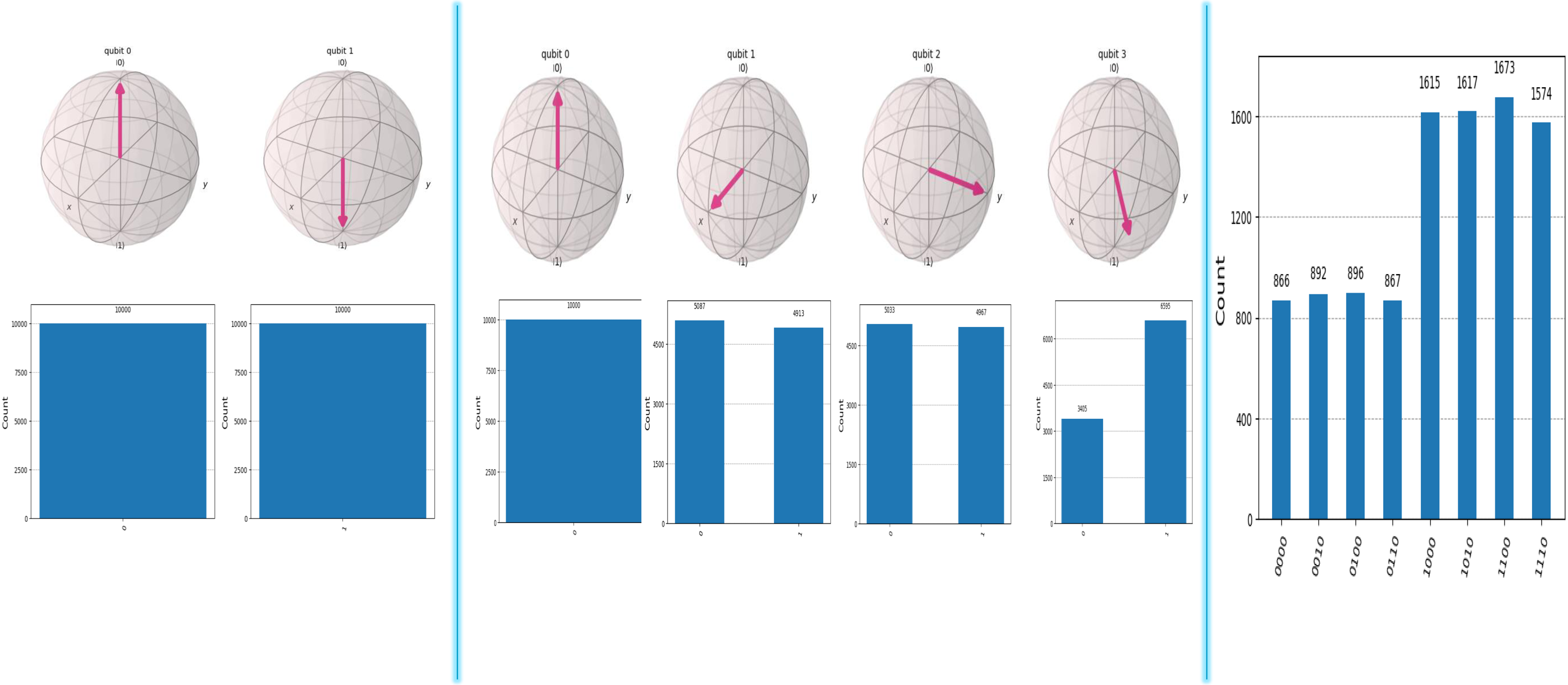
Now, shift your eyes to the middle of the slide. Here, we enter the quantum world. A qubit can sit anywhere on the surface of the sphere, not just the poles. Its position is determined by two angles, a bit like latitude and longitude on there, and that pair of angles determines, uniquely, where it is and its state. When we measure a qubit, the result depends on where it was on the sphere’s surface. If it is exactly on the pole, it behaves just like a classical bit, always zero or always one, but if it lies on the equator, it is what we call equal superposition, a perfect 50/50 mix, just like flipping a fair coin; half the measurements give zero, half give one. You can see that in the middle two histograms in the middle pane, where the outcomes are roughly 50/50 between zero and one.

Now, look at the right-most qubit, which is in the southern hemisphere, closer to the one pole. That means, if we measure this qubit many times, it will return one more than often than it will return zero. We can see, in fact, that is the case. The histogram shows about 70% probability of landing in one state compared to zero.

Finally, on the far right, we combine all four qubits. The x-axis now shows every possible four-bit outcome, according to this combined state, from 0000 to 1110, and bar heights show how often each qubit appears at the south pole when we measure the whole system.

Notice something interesting: every label on the x-axis ends with a 0. That’s because the first qubit, over on the left, was fixed at the North Pole – it is always zero. Notice something else. If we add up all the bars where the bottom bit is one, we will get roughly 70%, which matches the probability we got for the fourth qubit on the right. That is how the ensemble behaviour reflects what is happening at the multi-qubit level.

In short, classical bits are all or nothing, qubits can exist in mixtures of states until observed and measurement converts those quantum probabilities into classical outcomes. Superposition is what allows quantum computers to explore many possibilities simultaneously. Think about the poll question: 3 classical bits can encode eight different possibilities but only one at a time. Superposition allows all eight possibilities to be encoded simultaneously, with a particular probability attached to each.

[The speaker conducted another online poll, as shown in Figure 2.]

Figure 2.

Audience poll.

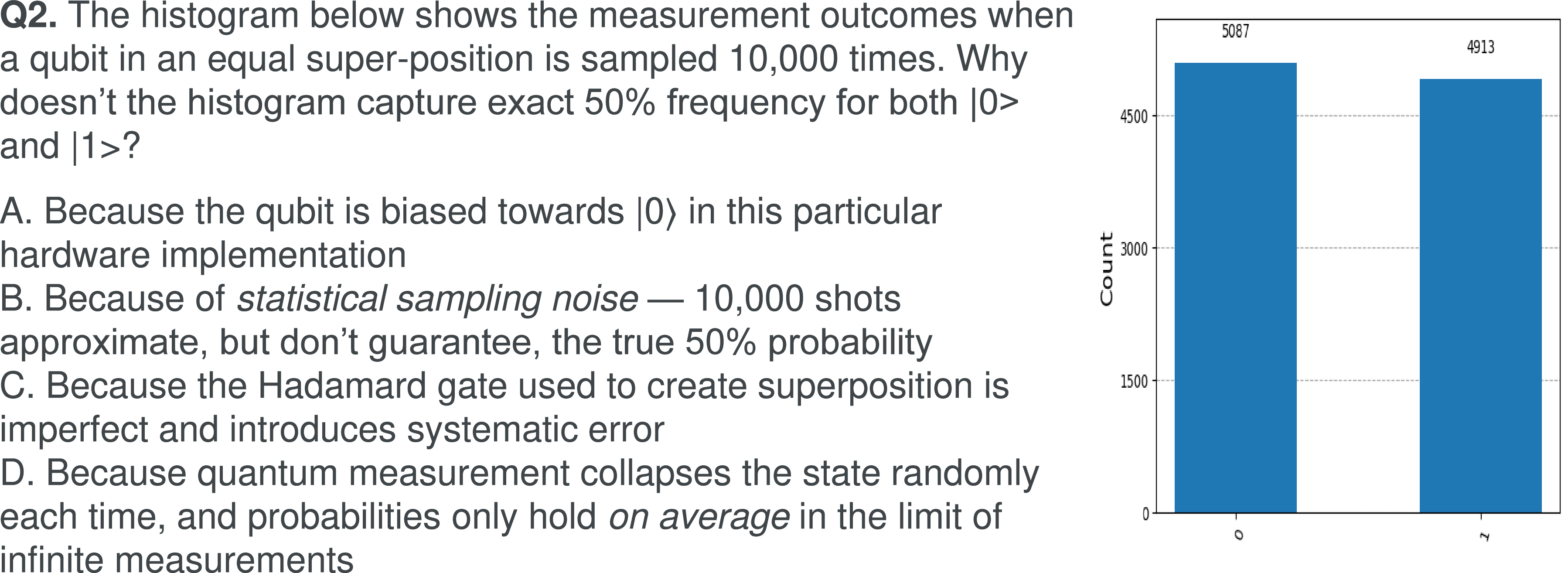
The results are that 57% of respondents chose B and 34% D. Options B and D are the right answers. Even though the qubit has an equal superposition of zero and one, quantum measurement is inherently probabilistic. Each measurement randomly collapses the qubit into one of the two basis states, with probabilities of 50%, on average. When we take a sample of 10,000, what we are seeing is statistical sampling. It is just like flipping a fair coin 10,000 times, not getting exactly 5000 heads or tails. The law of large numbers ensures that the result approaches 50/50 only in the limit.

The other thing I want to mention is that, unlike classical simulations, which use pseudo-random number generators, which can be seeded to reproduce the same sequence, quantum randomness is true physical randomness. It cannot be seeded, repeated or predicted. Every run is genuinely unique because it emerges from the underlying laws of quantum mechanics themselves.

Let’s move on to something that even Einstein found unsettling, what he famously called “spooky action at a distance.” Einstein disliked what quantum mechanics seemed to imply about the nature of reality, that the fundamental building blocks of nature are indeterminate until measured and that two particles, say, electrons or photons, can become so deeply linked that measuring one instantly tells you something about the other, no matter how far apart they are. That phenomenon is called Entanglement.

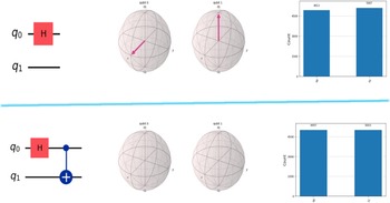
From an actuarial or financial modelling perspective, you can think of Entanglement as a sort of correlation between qubits, something that can help us capture the dependency structure of a copula. Physicists might take offence at what I am saying, but what we are talking about today is the practical utility of this correlation, rather than the deeper philosophical base for it. You notice a different type of diagram in Figure 3, which has wires in boxes. These are called quantum circuit diagrams, and they are the standard way of representing how qubits evolve during a computation. Each horizontal line represents a qubit. Think of it like a timeline of that qubit’s life. The boxes on those lines are called quantum gates – the operations we apply to change their state. Let’s start with the top half of the slide. We have only two qubits, labelled Q0 and Q1. Only the top one, Q0, passes through a red box with an H on it. That is called a Hadamard Gate.

Figure 3.

Entanglement.

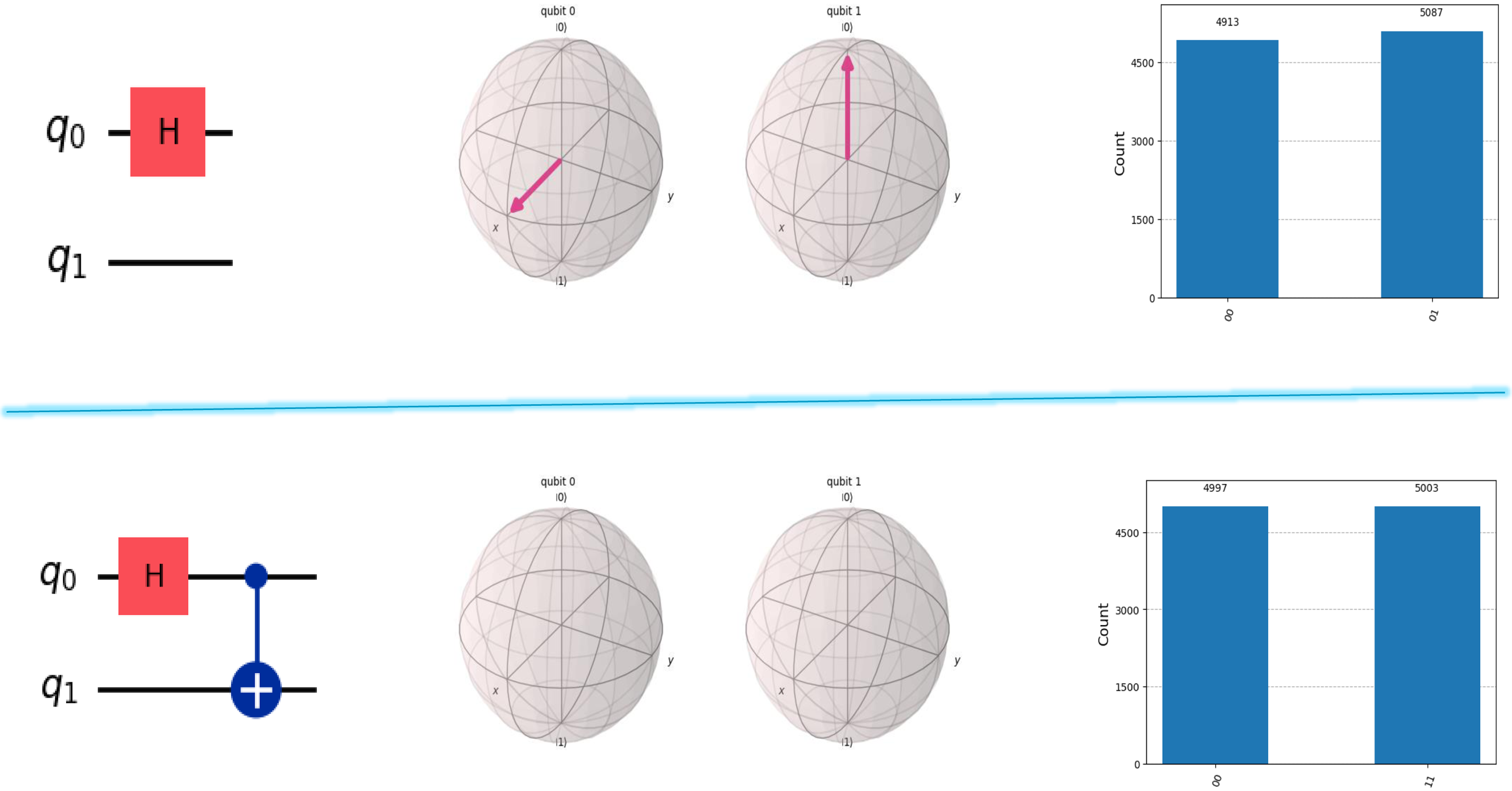
The Hadamard Gate takes Q0 from a definite north pole, that is, zero position state, to an equal superposition of zero and one, that is, on the equator. The second qubit, Q1, has not been touched. It is still sitting at the north pole. Because these two qubits have not interacted, they are not entangled. They are independent of each other. When we measure them, which is shown in the histogram on the right, Q0 collapses to zero or one, with equal probability, whereas Q1 is always zero. If you look at the x-axis labels, you will see “00” and “01”. Starting from the top, you read “00” and “10”. The top qubit is in zero 50% of the time and in one 50% of the time, whereas the bottom qubit is always zero, as we expected.

Now let’s move to the bottom pane, where we create entanglement between the two. We start in the same way, Q0 goes through a Hadamard gate to enter superposition, but now we have added a wire, connecting Q0 to Q1, leading to a blue circle with a plus sign. That blue circle with a plus sign is called a CNOT gate, short for controlled-NOT. What it does is, if Q0 is state one, then it flips the state of Q1, otherwise, it leaves it alone. That single operation creates entanglement between the two qubits. The two qubits are now linked. They no longer have independent probabilities, as you can see in the histogram on the right. The outcomes are now 00, with 50% probability, and 11, with 50% probability, that is, they both share the same state in each measurement. This is the simplest form of entanglement, called a Bell pair. Just as we use controlled-NOT gates to create perfect correlations, we can introduce partial correlations by using controlled rotations with different angles, where the strength of that link depends on the rotation angle itself.

Think of the Bloch sphere analogy again. The controlled-NOT gate rotates the target qubit from being at the north pole to the south pole. If the control is already at the south pole, that is 180 degrees (or pi radians) rotation. In fact, we could have chosen any other rotation angle. That is how quantum circuits can represent not just independence or full dependency, but a continuum of correlation strengths, a concept that might seem familiar to anyone who has calibrated copula models.

Now that we have built some intuition about superposition and entanglement, let’s see how those ideas translate into actual computation. Any computation, classical or quantum, starts with encoding a problem into hardware and then manipulating that hardware according to certain rules. In the classical world, we rarely think about this anymore. Layers of software are abstracted away and we just write C code or Python code or MATLAB code or R code, and so on. But underneath, everything is reduced to binary instructions, streams of zeros and ones being manipulated through Boolean logic inside transistors. Quantum computing is similar in spirit; but here, instead of binary states, we are working with quantum states, which can exist in superpositions. We need a way of encoding those states mathematically and geometrically.

If you look at the top part of Figure 4, you will see the canonical mathematical form of the qubit’s state. We write it as “psi is equal to alpha times state zero plus beta times state one,” where alpha and beta are complex numbers. They are also called probability amplitudes.

$$\left| \psi \rangle\right. = {\rm{\;}}\alpha \left| 0 \rangle\right. + \beta \left| 1 \rangle\right.$$

Figure 4.

Encoding.

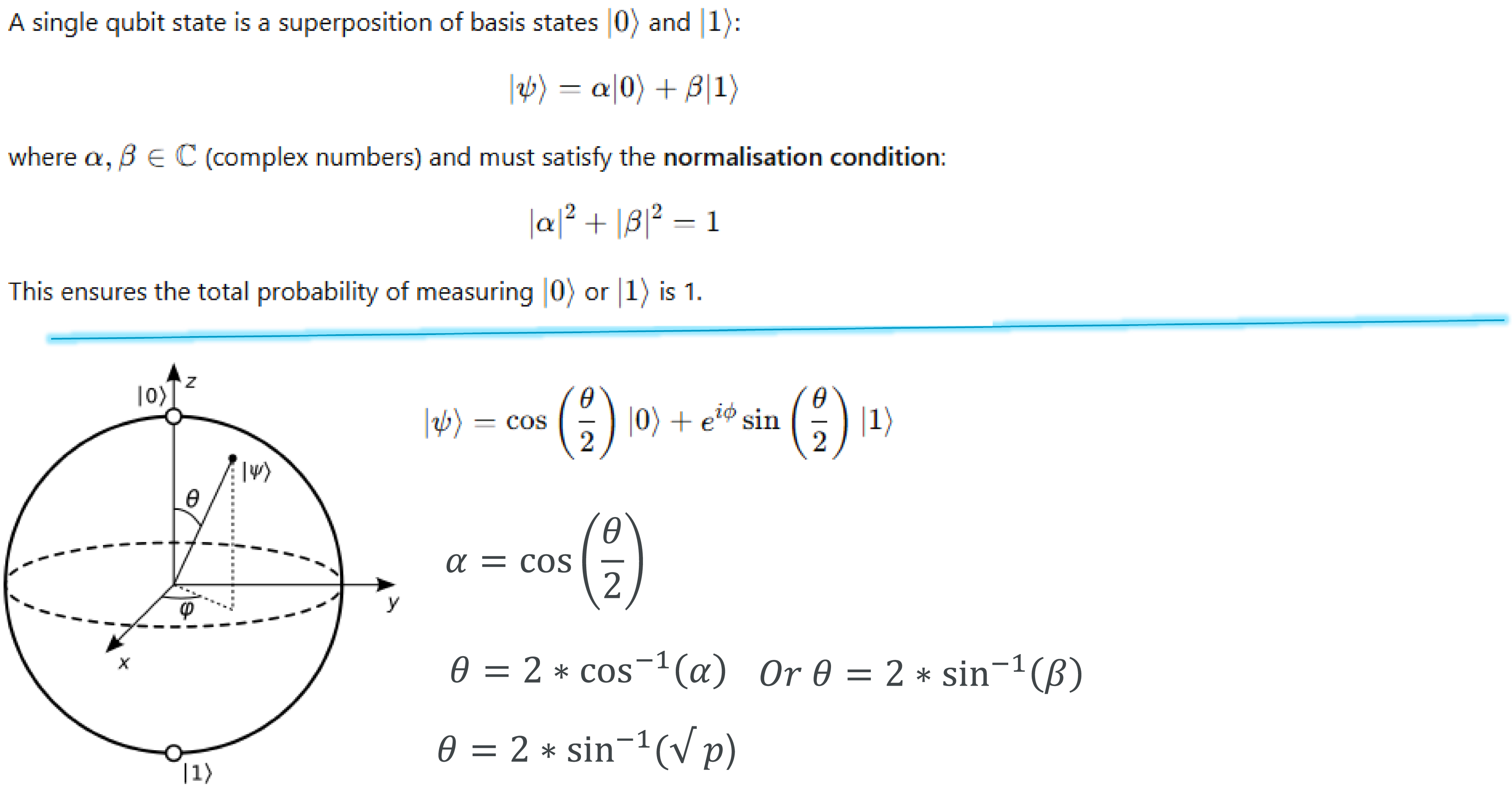
To make sense, probabilistically, they must also satisfy the normalisation condition, which is that the sum of their squares should be equal to one. Alpha and beta are not probabilities themselves. They are amplitudes whose squares give us the probabilities.

Let’s move to the bottom half of the chart, which gives us a geometric way to visualise these same relationships. Any single qubit state can be represented by a point on the surface of this sphere. Angles theta and phi (think of them of latitude and longitude) determine exactly where the state lies. Mathematically, we can express the qubit state as:

$$|\psi\rangle = \cos\left ({{\theta}\over{2}}\right)|0\rangle + e^{i\phi}\sin\left(\frac{\theta}{2}\right)|1\rangle$$

Here is the key takeaway: theta determines how far the qubit is tilted away from the north pole, and therefore controls the probabilities of measuring zero or one. Phi, on the other hand, controls the phase, the orientation of that state around the equator. If we measure this qubit repeatedly, only theta affects the outcomes – the likelihood of zero versus one. That is why theta is what we usually use for encoding probabilities. The phase phi is invisible to direct measurement, but it plays a crucial role later. It governs interference, which is how quantum algorithms amplify correct answers and suppress incorrect ones. In short, theta encodes how likely an outcome is, and phi encodes how those probabilities interact when we combine the qubits. This gives us a simple way to visualise qubits. We see that, by rotating a qubit, we can encode any probability we like into it. I have shown the inverse cosine and inverse sine relationships between the probabilities and the theta.

Now that we have seen how a single qubit can represent probability distribution over two states, zero and one, let’s scale up to see what happens when we have multiple qubits.

As mentioned before, the size of the states base grows exponentially with the number of qubits, specifically two to the power of n. With one qubit, we have two states: zero and one; with two qubits we can represent four states: “01”, “01”, “10”, “11”; and with n qubits it is two to the power of n possible combinations. Each of these states is what we call a computational basis state, and each has an associated probability amplitude, which could be zero, as we saw in the entanglement example, where the states 01 and 10 never appeared in our histograms because we only ever saw 00 or 11. Look at the top half of Figure 5. This diagram shows what is called the probability branching or binomial tree method for encoding any arbitrary probability distribution across the multiple qubits we have. Our target quantum state is shown at the very top, which is psi is equal to square root of 0.2 times 00, square root of 0.3 times 01, square root of 0.25 times 10 and square root of 0.25 times 11; which means that we want 00 to appear 20% of the times, 01 to appear 30% of the times and 10 and 11 to appear 25% of the times:

$$|\Psi\rangle = \surd{0.2}|00\rangle + \surd{0.3}|01\rangle + \surd{0.25}|10\rangle + \surd{0.25}|11\rangle$$

Figure 5.

Dense encoding.

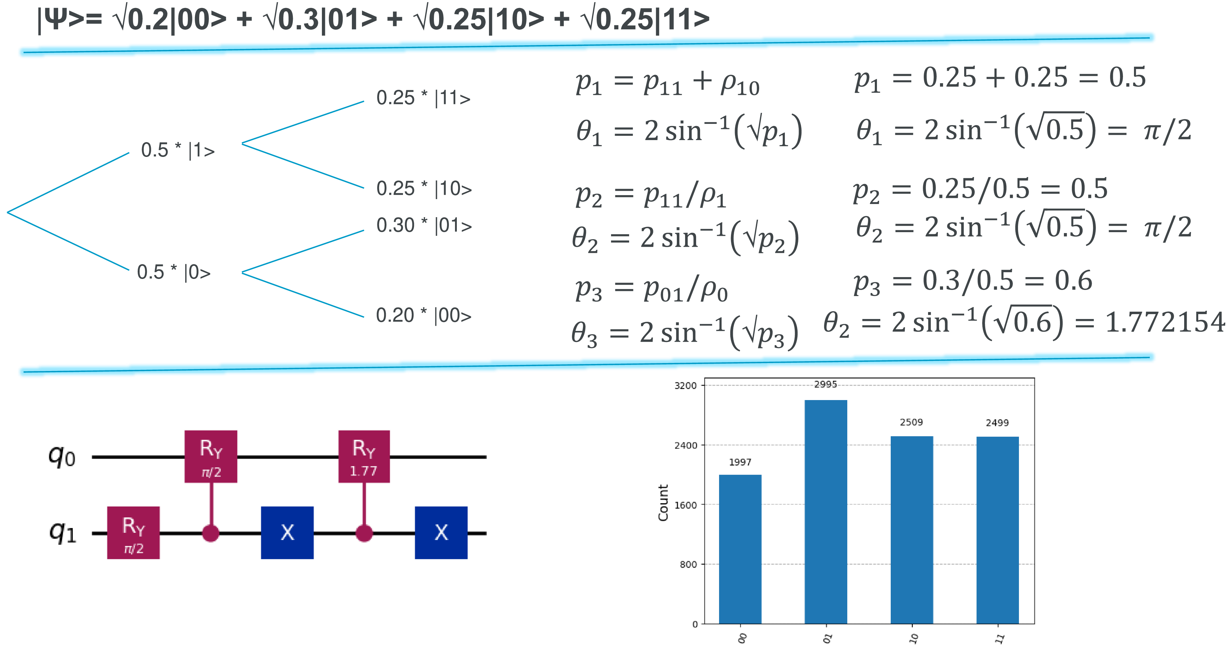
To achieve this, we can think recursively. Each level of the tree represents a qubit, and each branch represents a conditional probability, given the qubits before it.

In this example, we have three degrees of freedom. We can freely set three probabilities and the fourth is automatically fixed because the total must sum to one. Let’s walk through how we compute these rotation angles. We start with the left-most qubit, Q1. The left-most qubit is Q1 because of the convention used by Qiskit, which is the Python library I have used here. To find its probability of being in state one, we essentially add up all the probabilities of all states starting with one. In this case, we know that 10 and 11 end up with this left qubit being in state one. We will sum those up and we will get 0.25 plus 0.25 equals 0.5, which is our equal superposition state. Remember that translating the state from the north pole to the south pole was pi radians rotation, so going to the equator is pi upon two, so we get pi upon two over here.

We move on to the second rotation. For this one, we condition that Q1 is equal to one because we worked that out already and we are in the top branch, and look at the right qubit, which is Q0. We will take the ratio of the joint probability of both qubits being in state one and the unconditional probability of qubit one being in state one, which is 0.25 divided by 0.5, which, again, gives 0.5, so a pi upon two radians rotation again. For the third rotation, we move to the bottom branch, where Q1 is equal to zero. We will take the ratio of the joint probability for the second branch being in an up-state, while the first branch is in the down-state, which is 0.3 divided by 0.5, which gives us 0.6, or in other words, 1.77 radians rotation, as we worked out through this inverse sine relationship.

Bloch spheres and rotations are very useful for visualisation and to help us to develop an intuition, but they are not actually how we program quantum computers. The bottom half of Figure 5 shows how we would program the above using a quantum circuit. I want to look at the circuit diagram. Each magenta box is a rotation through the y-axis, which rotates by an angle theta (again, remember latitude and longitude). The blue boxes are X-gates or gate flips. Essentially, they flip the state of the qubit. If you are at the north pole, they will move you to the south pole, and the connecting lines indicate controlled rotations, which we have seen before. Previously, we saw the controlled-NOTs. These are controlled Y-rotations, which can encode partial correlations and so on. The binomial tree above directly matches the circuit. You will see both Q1 and Q0 start off at the north pole because they initialise to zero. We apply a pi upon two rotation around the y-axis to Q1. This puts Q1 on the equator, that is, equal superposition. There is then a controlled Y-rotation of pi upon two radians, going from Q1 to Q0, essentially saying, “If Q1 is one, make Q0 also 50/50,” which is the top half of the probability tree.

Applying an X-gate will then switch it, moves us to the bottom half of the tree because now we are saying, “If it is zero, make it one.” If we start off in this state, which is zero, applying the X-gate will make it one and allow us to control the behaviour of this target qubit. We can now apply the controlled Y-rotation again, which was the theta three that we worked out from our binomial tree. We then run this circuit, and we find that it reproduces the probability distribution that we had at the top, so (00, 20%), (01, 30%), (10, 25%) and (11, 25%).

This method is conceptually neat and intuitive, but it is not the most practical method for real quantum hardware because it requires an exponential number of gates, specifically two to the power n minus one rotations. In this example, we had two qubits, and we needed three angles, so two squared minus one gives us three. For three qubits, we would have needed seven, and so on. That becomes very heavy, very fast. In practice, quantum libraries use more efficient encoding schemes, such as grey code, which is implemented out-of-the-box in Qiskit. I chose binomial tree here because that is more familiar to an actuarial audience. The key takeaway is that, in principle, we can encode any probability distribution across qubits. The challenge is doing so efficiently.

Moderator: A question has been posted relating to Figure 4. I thought you had best answer it now, before you move on to the internal model material. In entanglement, can change in Q1 affect Q0 or is it one-way only?

Mr Amjad: It is both ways. It is not in the scope of today’s talk, but in the quantum realm, causality is not one-way as it is in the classical realm. You cannot speak about one influencing the other, because they become entangled. They are virtually indistinguishable from one another. It does not matter which one you are measuring. You know when you measure the other one, it will yield exactly the same outcome.

[The speaker conducted an online poll, asking the question, “A 32 GB RAM classical computer can simulate ∼30 qubits. Roughly how many qubits could 64 GB handle?” 31% of respondents chose the correct answer, which was 31 qubits.]

Remember, this is related to that exponential state base increasing. Each additional qubit doubles the amount of memory needed for simulation because the quantum state has two to the power of n complex amplitudes to keep track of. So, if 30 qubits require 32GB, then 31 would require 64GB, 32 would require 128GB, and so on. To put that in perspective, simulating the caffeine molecule, which has around 95 electrons, would require tracking over two to the power of 95 amplitudes, which is far beyond the capacity of any classical computer on earth. It might be greater than the number of atoms we have in the universe as well. This exponential scaling is why we can only simulate a few dozen qubits classically and why real quantum hardware, even with its noise and imperfection, is so valuable for exploring quantum behaviour directly.

Let’s move on to Figure 6, which you might have seen in the paper and in The Actuary article.

Figure 6.

Dense encoding.

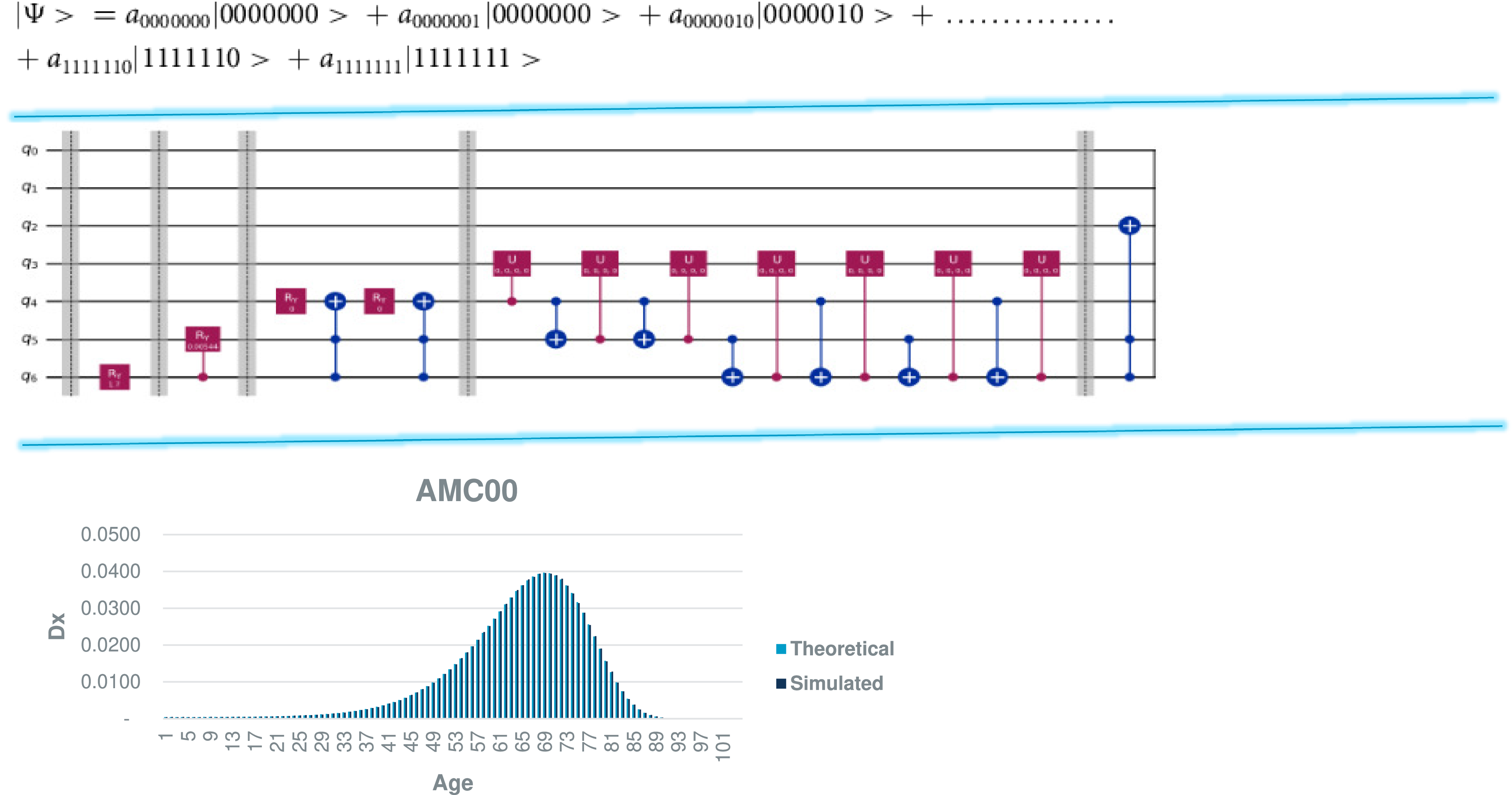
This case is just the AMC00 mortality table encoded into a set of qubits. I have used seven qubits, because two to the power of seven gives us 128 possible states, which is enough to represent ages all the way from zero to 120, each associated with its own mortality probability. The canonical form at the top shows the general form of the qubit’s quantum state and a superposition of all the possible bit strings, from 000000 all the way to 111111. Each of those quantum amplitudes corresponds to the encoded mortality probability for a specific age. The quantum circuit in the middle is the result of applying the dense encoding algorithm I showed before, the sequence of controlled rotations that embed those probabilities directly onto the amplitudes of qubit system. It is conceptually like the probability branching approach, but uses conditional rotations and shared gates, which is just a way of compressing the encoding and reducing the circuit depth. Finally, the chart at the bottom compares the theoretical mortality probabilities from AMC00 with the simulated probabilities recovered by repeated measurement of the quantum system. You can see that the two align very closely.

Let’s take a quick detour to the more familiar actuarial territory of Solvency II IMs, just to make sure we are not losing those who have not worked on IMs before. What is an IM for anyway?

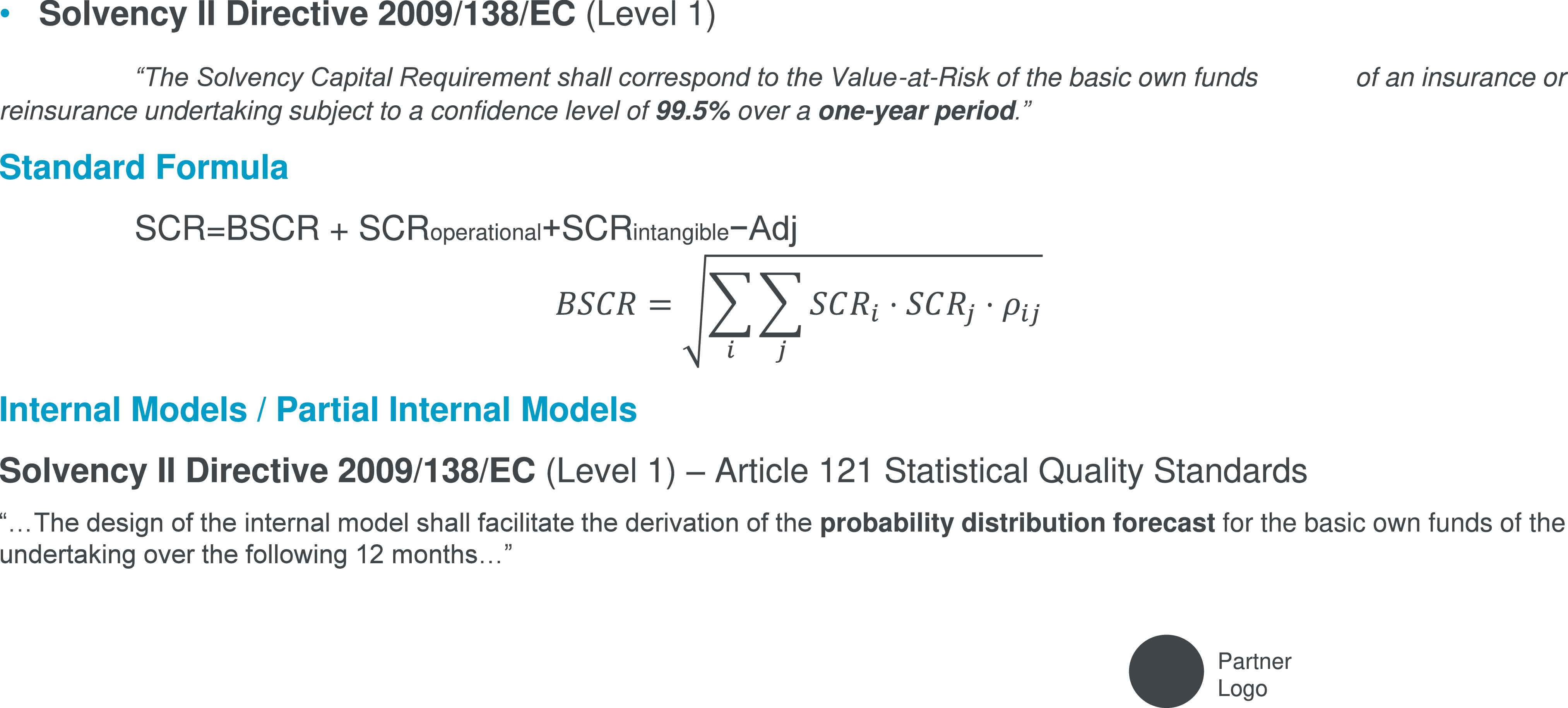
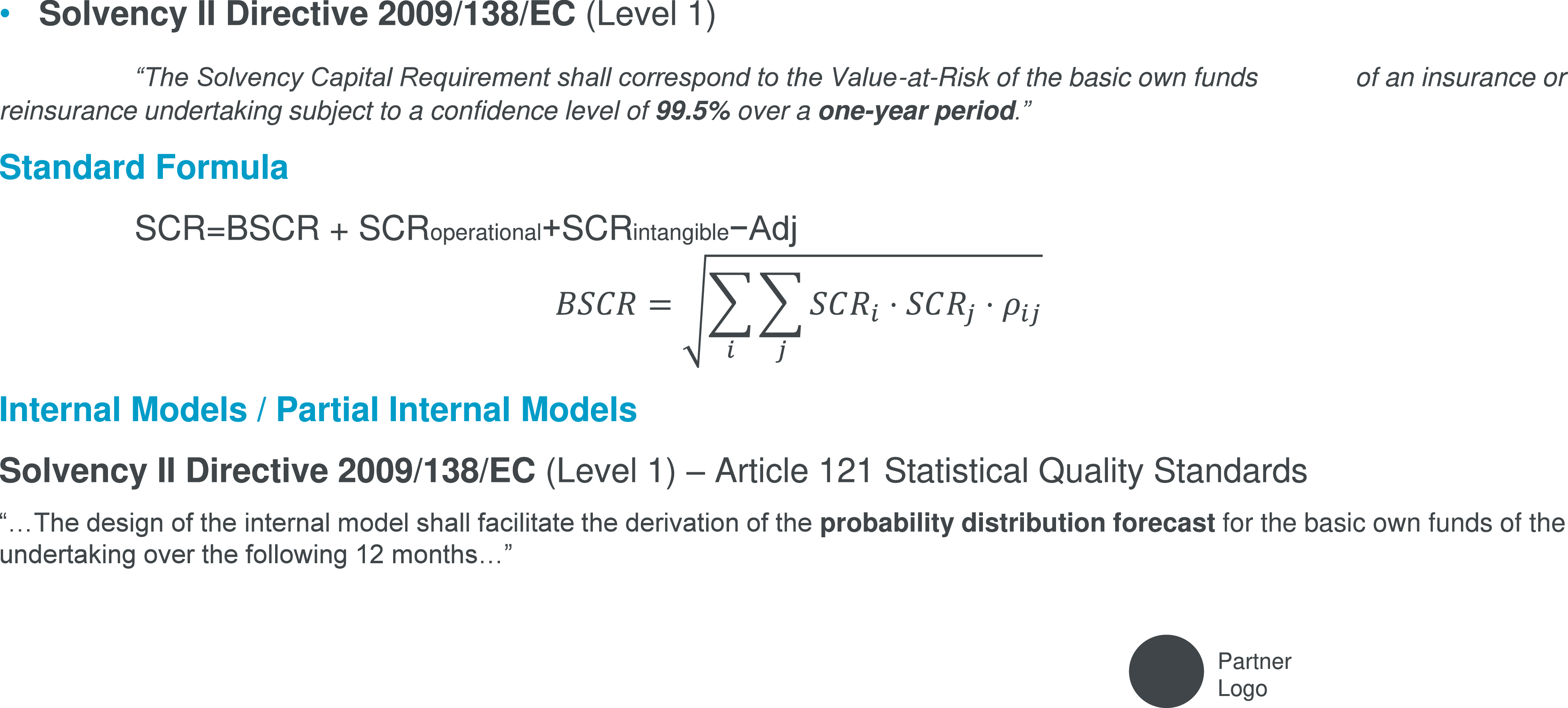
Figure 7 references the Solvency II directive, essentially saying that the insurance entities need to hold capital to cover them for a 99.5% tail event, also colloquially known as the worst event in once every 200 years. Firms can calculate this value-at-risk using the Standard Formula, or they can develop IMs. One of the requirements, from an IM perspective, is that it should facilitate a derivation of a probability distribution forecast for Basic Own Funds, which naturally has resulted in most firms developing stochastic IMs, although there are some exceptions. Although many firms differ in detail, the overall design of stochastic IMs is remarkably consistent across the industry.

Figure 7.

What is an internal model for?

You can see the structure illustrated in Figure 8. We start on the left-hand side with a set of individual risk modules, for example equity, interest rates, credit spread, inflation and so on. Each of these is typically calibrated by fitting a parametric probability distribution to historical data or by using expert judgement. For instance, fitting a lognormal distribution to equity returns or a t-distribution to credit spreads.

Figure 8.

Internal model schematic.

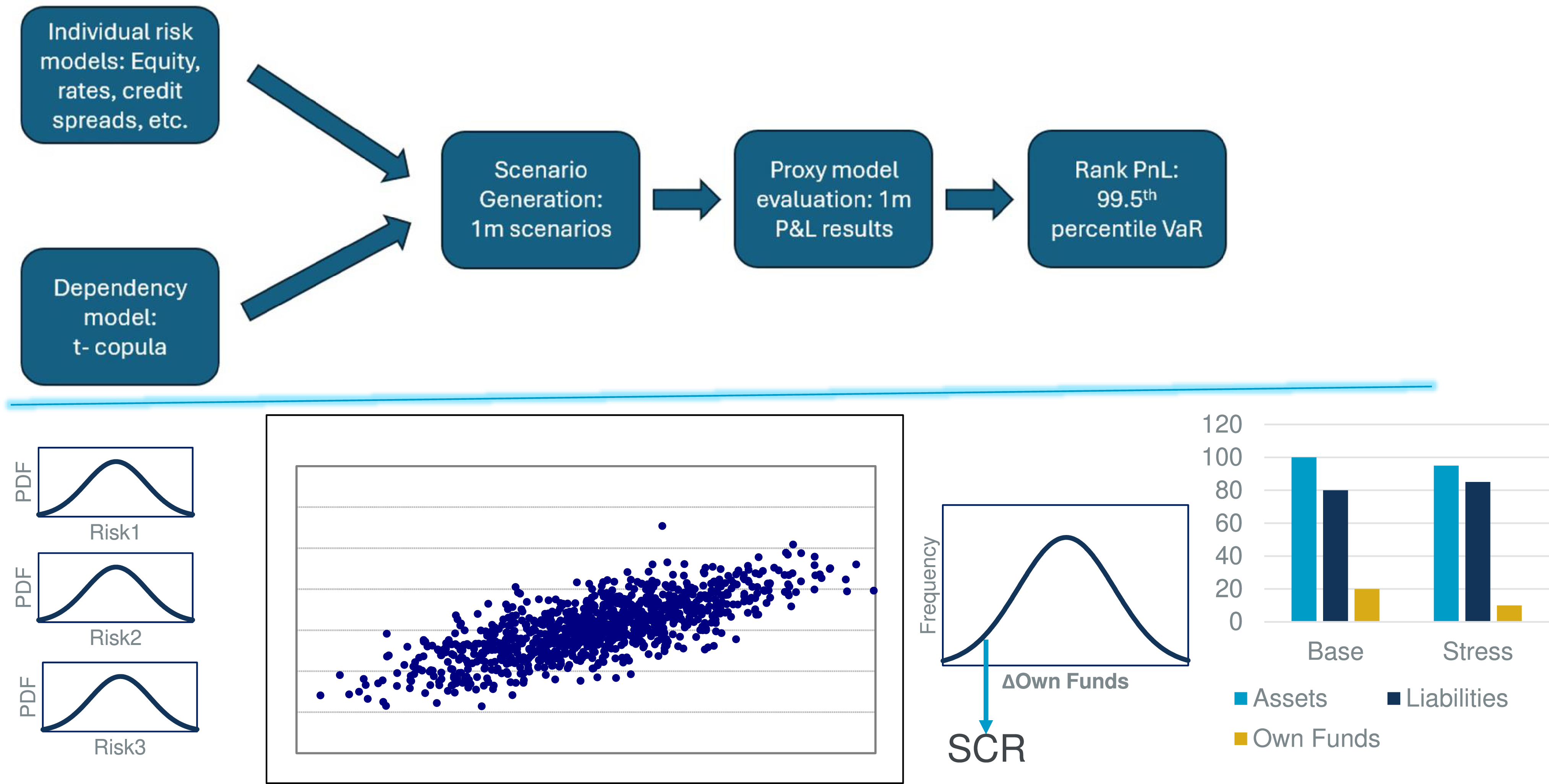
Next, these individual risks are essentially stitched together using a dependency model, most commonly a Gaussian copula or a t-copula. Between these, they define the joint behaviour of all risk factors, their correlations, their co-dependencies, and together they form the scenario engine for the IM. Moving one step to the right, the model then simulates hundreds of thousands, often half a million or a million, simulations or stochastic scenarios. Each scenario represents a possible future realisation of the entire risk universe over a one-year horizon in line with Solvency II requirements. Those scenarios then feed into a proxy model, which re-evaluates the balance sheet under each of these stochastic simulations, producing, let’s say, half a million simulated Own Funds outcomes. Once we have that full distribution of Own Funds, we simply rank the results and take 0.5th percentile. That is our 99.5th percentile value-at-risk or SCR requirement. You can see the process visualised along the bottom. On the left, we start off with the marginal distributions. The scatter-plotting in the centre shows how these individual risks combine under the dependency structure, and on the right, we have the resulting distribution of changing own funds. We identify the SCR as the drop-down from the base to that 0.5th percentile point. Finally, the bar chart illustrates what happens to the balance sheet in that stress, that is, assets fall, liability rise and Own Funds reduce, and that reduction in Own Funds corresponds exactly to the SCR.

So, that is the classic architecture: marginal risk distributions, dependency via copula, scenario generation, proxy evaluation and then the extraction of the 99.5th percentile. In a few slides, we will revisit the schematic to explore quantum magic. Before we do that, we still need to cover a few more concepts. While we have seen how the risk distribution or the dependency can be encoded, what we have not yet tackled is the balance sheet evaluation. That is where proxy models come in. As many of you know, full cash flow models are often too computationally expensive to run under hundreds of thousands of scenarios, especially for complex products, like with-profits funds where the costs of guarantee already requires stochastic models just for the base valuation. To make that tractable, the industry has turned to proxy models, essentially polynomials calibrated to approximate how the balance sheet behaves under different stresses. Instead of revaluing every asset and liability using the cash flow model, we evaluate a simple function, a polynomial that captures key sensitivities.

Let’s walk through a simple example to see how we can represent a polynomial on a quantum computer (Figure 9).

Figure 9.

Quantum proxy models.

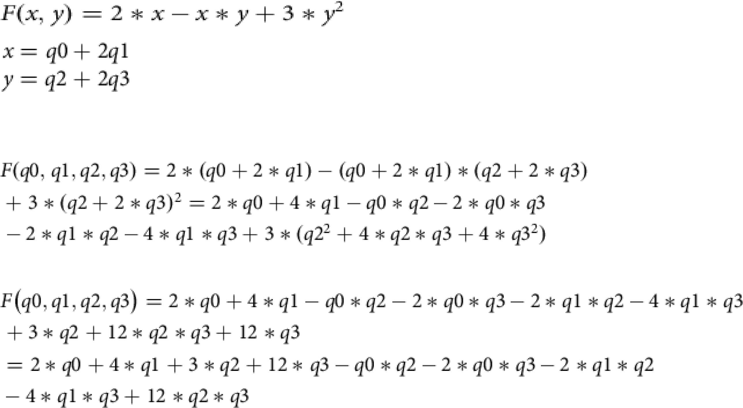
In this case, we start with a simple function, “f of xy is equal to 2x minus xy plus 3y squared.”

It depends on two risk factors, x and y, and it has three terms, one linear in x, one cross-term between x and y, and one quadratic term in y. Since each of these risk factors has its own probability distribution, assuming two qubits we can represent each using Q0 and Q1 for x, and Q2 and Q3 for y. Each pair of qubits represents four possible outcomes, 00, 01, 10 and 11, which, if we convert from binary to integer format, simple corresponds to zero, one, two and three. You can think of these as your risk factors. That means we can express x as equal to Q0 plus two Q1, just converting from binary to integer format; and the same for y, which is equal to Q2 plus two Q3. We substitute these expressions for x and y into our polynomial. That gives us a new function, f of Q0, Q1, Q2 and Q3, which expresses the balance sheet proxy model directly in terms of qubit states. Here is one important simplification. Since upon measurement the qubit state collapses to a classical binary outcome, that is, zero or one, squaring it just gives it the answer. It doesn’t change. In other words, Q0 squared is equal to Q0. Q1 squared is equal to Q1, and so on. That makes the algebra slightly neater but notice what has happened when we expand everything out. We have gone from three terms in risk factor space, to essentially nine terms in qubit space. In effect, we have taken a simple polynomial and exploded it into multiple quantum components. To represent all of this quantum mechanically we will need at least nine qubits in our circuit: four qubits (Q0–Q3) to represent x and y, our risk factors; and an additional five qubits to represent all the cross terms. We should remember each also carries a coefficient, as you can see here, which will also need to be encoded.

[The speaker conducted an online poll, as shown in Figure 10. Most respondents chose the correct answer, which was “C”.]

Figure 10.

Audience poll.

Every term in the polynomial, especially the high-order interactions, needs its own qubit representation. To give you an example of the QIM I built, it had 834 terms and it was a fifth-order proxy model. It ended up requiring over 35 million qubits, which gives you a sense of how quickly things blow up.

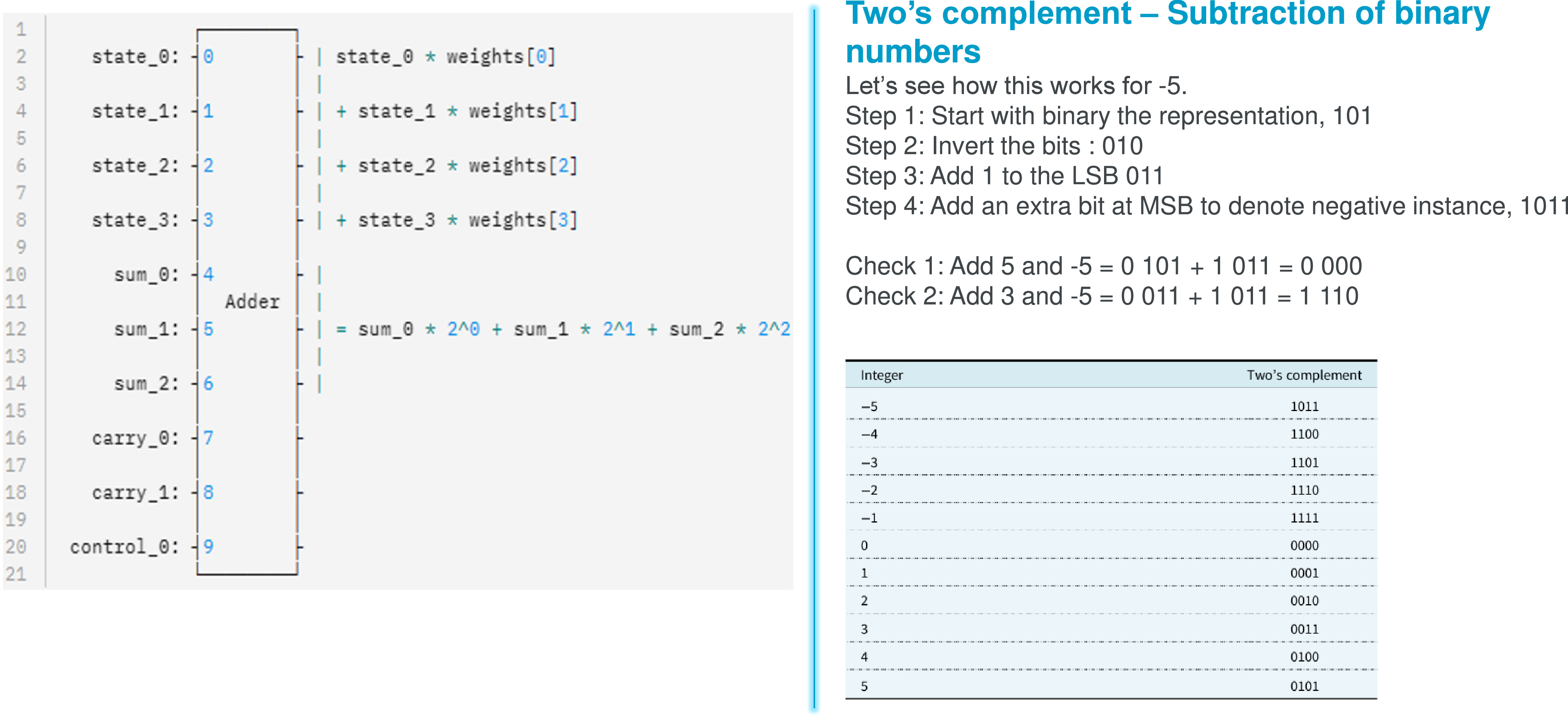
As I mentioned on the previous slide, each of the interactions will need to be encoded. Each term has a coefficient attached to it, which will also need to be encoded. That is where this weighted adder circuit helps us to evaluate the polynomials. The key takeaway is the weighted adder circuit allows us to compute a weighted sum of qubit states, which is important because we need to capture the qubit coefficients, not just the qubits themselves, which is why it is exactly what we need to evaluate the polynomial proxy model we just derived. However, there are a few practical considerations we need to look at. Firstly, it only accepts positive integers as weights. If our polynomial coefficients are not integers, we need to have a new strategy, but this is a simple problem to solve. We can simply rescale them by multiplying all coefficients by a reasonably high power of ten until they all become integers and then scale it back down in the post-processing phase.

The other limitation of the weighted adder circuit is that, because it only takes in positive weights, we need a way of handling negative weights. We do that by splitting the computation into two branches – a positive branch and a negative branch. Each branch computes its own weighted sum and then we subtract the negative branch from the positive one. The subtraction itself uses a method called Two’s complement, which is shown on the right-hand side of Figure 11. In essence, instead of having a separate minus operation, we represent a negative number in Boolean algebra, by inverting its bits and adding one. This trick lets the subtraction be performed as an addition, which is far easier to implement in both classical and quantum logic circuits. I provided some work examples on the slide. With a combination of rescaling and the Two’s complement subtraction, the weighted adder can efficiently handle the full range of coefficients in a proxy model, allowing us to compute the weighted sums directly within a quantum circuit.

We have looked at all the building blocks, so we have got everything we need to build a QIM. We have looked at a way of encoding risk distributions. We have looked at the ways of encoding dependencies. We have looked at how we can perform arithmetic and implement proxy models. Let’s combine them and see what this naïve QIM would look like. I call this naïve not because it is wrong, but because it is a direct translation of the classical calculation into quantum form, without yet exploiting any quantum algorithms for speed up or efficiency.

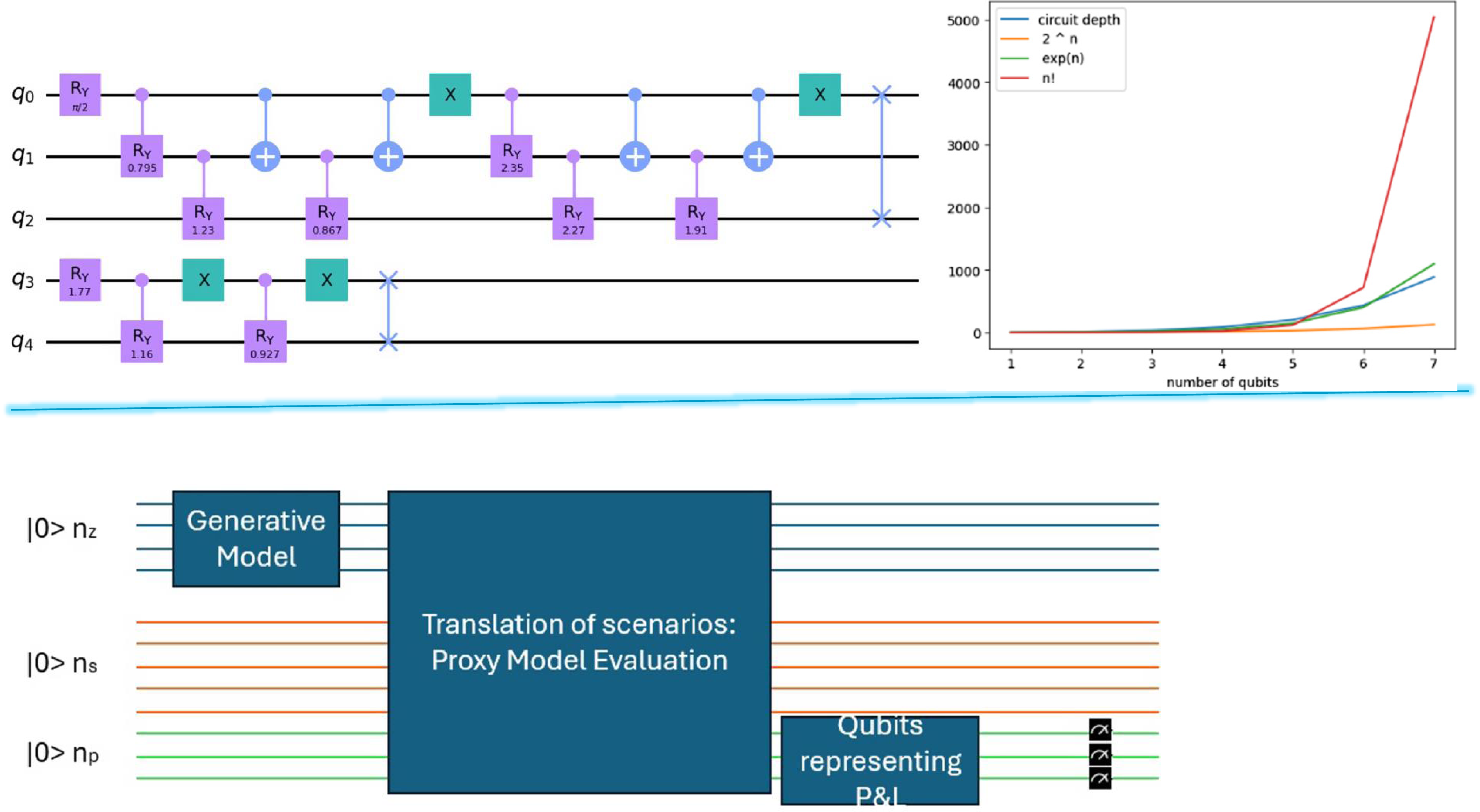
At the top of Figure 12, you will see a basic example of a risk distribution being implemented on a quantum circuit. Each purple box is a rotation gate, setting the amplitudes to match our desired probability distribution, and the blue plus and X symbols are controlled operations, or controlled-NOTs, that we have seen before. On the right-hand side, the graph tells us an important story. As we increase the number of qubits to encode our distributions, the circuit depths, effectively the number of gates, grow exponentially. You can see that the red curve is rising sharply. By the time we reach just six or seven qubits, the gate counts shoot into the thousands. That is the same scaling behaviour we have seen in other dense coding examples. It illustrates how naïve implementations hit hardware limits very quickly. In the bottom schematic, we have the architecture of the full QIM, but the naïve version. We start with a generative model. The middle block is called the translation of scenarios, or proxy model evaluation, which is where we compute our change in Own Funds. You will see some red lines running through it in the middle. These represent the additional qubits we needed to handle the polynomial interaction terms, the weighted sums, the Two’s complement arithmetic, and so on. Finally, the green qubits at the bottom represent the evaluated change in Own Funds, which is what we are interested in. These green qubits are what we can measure directly to obtain a probability distribution of Own Funds, from which we can then extract the 99.5th percentile loss in Own Funds, exactly as we would in the classical IM realm. At this stage, everything works. We have shown that the full SCR process can, in principle, be reconstructed quantum mechanically. But, and this is the key point, so far we have achieved this without any quantum advantage.

Figure 11.

Quantum arithmetic.

Figure 12.

Naïve QIM.

Now we come to one of the most exciting and fun parts of this talk: the promise of quantum advantage for value-at-risk or SCR calculations.

Let’s start with the chart in the top left corner in Figure 13. This is what is called a convergence diagram showing how our estimate of value-at-risk changes as we increase the number of simulations and as we vary the random number seed used to generate them. Notice there is a shape to that funnel. As the number of simulations grows, the uncertainty around our estimate narrows, and the width of that funnel of doubt steadily narrows. This convergence follows a very familiar rule. The standard error decreases with one over the square root of N, where N is the number of simulations. If we want to halve the uncertainty in our SCR estimate, we must quadruple the number of simulations. That is what we call quadratic scaling. It is one of the key computational bottlenecks in Monte Carlo risk modelling. As I mentioned at the beginning of the talk, the quantum risk analysis paper by Stephan Woerner and Daniel Egger presents an approach to calculate value-at-risk more efficiently compared to Monte Carlo simulations. Essentially, their thesis is that you can achieve a near-quadratic speed-up when using quantum amplitude estimation (QAE) to estimate value-at-risk. To put this in perspective, it would be like achieving the same accuracy in your SCR using 1000 simulations instead of 1 million. My investigation, and what I am presenting today, was precisely to test whether this advantage only holds for toy problems like the one presented in the Woerner and Egger paper, or whether it could extend to industrial-scale IMs - the kinds used by firms for calculating the SCR.

Figure 13.

Quadratic speed up via quantum amplitude estimation.

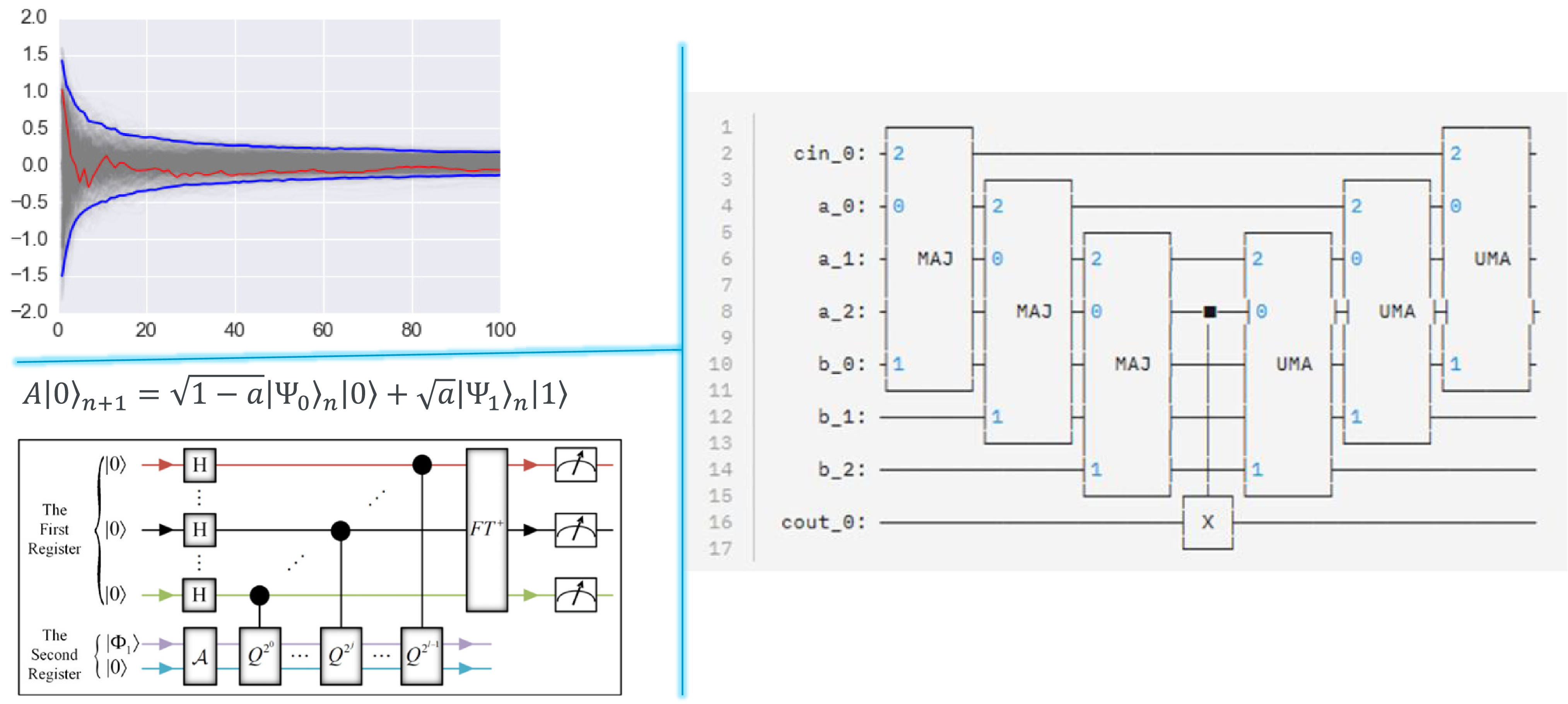
Before I move into the detail, let’s unpack the key idea behind QAE, which is shown in canonical form here in the bottom left of Figure 13. We begin with N+1 qubits all initialised in the 0 state. Then we perform some computation through a sequence of quantum gates. We evolve the system so it can be expressed in this form. Translated into plain English, it just says there is an operator, or a sequence of quantum operations or quantum gates, that we apply to a quantum circuit, such that there is some probability, A, of measuring the final qubit in state 1. That A corresponds to the amplitude of the outcome that we are interested in. There is the naïve way of estimating A through repeated sampling of the whole circuit, or the Monte Carlo method. But that is still subject to the 1 over square root of N scaling. If we use QAE, we can achieve the same accuracy with fewer samples. I know it is still a bit abstract. You might be wondering, how do we connect a single qubit’s amplitude to our usual delta NAV or SCR calculation?

Let’s take a step back and think about the diagram from Figure 12. Those green qubits represented the change in Own Funds. We do not want to sample them directly, as that would be the naïve approach we have spoken about. Instead, what we want to do is add a few extra qubits at the bottom and connect them in such a way that the probability of finding the final qubit in state 1 gives us information about the SCR. QAE then allows us to query this final qubit to estimate the SCR much more efficiently compared to Monte Carlo methods.

How can we do this? We can do this by encoding the threshold value in those extra qubits that we have added at the bottom, and by adding it to the green qubits, which represented our delta Own Funds. If the sum of these 2 registers, the green register and the extra register we added at the bottom, exceeds a particular value, there will be a carry on the final qubit and its state will change from 0 to 1. This set-up is called a comparator because it compares our delta Own Funds in the green qubits with this threshold and flips the final qubit if the threshold is exceeded. Let’s make this more concrete with a simple example.

Imagine we have 4 qubits representing our delta Own Funds. 4 qubits means 16 possible states, let’s say from 0 to 15 inclusive. Now, suppose we want to check whether the loss exceeds 7. In the comparative set-up, we do not add the threshold itself. We add Two’s compliment specific to the threshold, chosen so that if the loss is larger than 7, the sum spills over beyond what the 4 qubits can represent. I already said 4 qubits can represent values up to 15. We know if we add something to 7 which makes the sum 16 or above, they will be spilled, which means that we can encode 9 as our threshold, or the complement of our threshold. That carry qubit flips from 0 to 1 precisely when the loss exceeds 9. If the loss was any smaller, let’s say 5, the sum would stay below 16, and the carry would remain in 0. That is the intuition behind the ripple carry adder, which is the circuit shown on the right-hand of Figure 13. It is a standard quantum logic circuit that adds 2 quantum registers: you can see A0, A1 and A2; and B0, B1 and B2. When the sum overflows, a carry is generated. At the bottom you can see C-out 0. That is essentially what we can query for our QAE. When the amplitude for this threshold equals 0.5%, we found the threshold corresponding to the 99.5th percentile loss, that is, our SCR.

[The speaker conducted an online poll, as shown in Figure 14. 63% of respondents chose the correct answer, which was “B”.]

Figure 14.

Audience poll.

Hopefully, I am doing a reasonable job of explaining the concepts. I will walk through the explanation anyway. The key advantage of QAE is that it reduces the number of samples required to achieve a given level of accuracy. In classical Monte Carlo, there is square root scaling (square root of N) meaning that to halve the error, you need 4 times as many simulations. QAE, however, achieves the same precision with only a proportion to 1 over N samples, effectively a quadratic speed-up. It does not use faster random numbers or parallelisation, rather it exploits quantum interference to extract more information from each sample. As I mentioned, a classic model might need one million simulations, a quantum model could, in theory, achieve similar accuracy with something of the order of 1000.

I am conscious that the previous example may still not be clear enough. How do we connect it to this random distribution that we generate? I thought it might be worth walking through a comparator circuit example in the IM context. I mentioned that the comparator circuit is the key component that lets us test whether a simulated loss exceeds a given threshold. It is this mechanism that flips the final qubit state one whenever that threshold is achieved. Our task is simply to query that information efficiently using a threshold comparison.

We start with a circuit on the left in Figure 15. This example uses the ripple carry adder available in Qiskit out of the box to perform that comparison. I have shown that ripple carry adder circuit previously. Q0 is the carrying qubit, which we can ignore for this example. Q1 to Q5 encode random variables distributed over the range 0–31. That is because 2 to the power of 5 is 32, so 0–31 gives us our 32 possibilities. Q6 to Q10 hold the Two’s complement of the threshold we want to use for comparison. In this case, if you read from Q10 all the way to Q6, where there is no box that would correspond to a 0, because everything is initialised to 0. These Xs mean their states have been flipped, so they represent 1s, so we read 0, 1, 0, 1, 0. That represents N. Because our register can only represent values up to 31, adding 10 causes an overflow precisely when the variable exceeds 22, because 10 plus 22 is equal to 32. That overflow flips the carry qubit, the final qubit, from 0 to 1. In other words, this sets up tests whether the loss has crossed the threshold of 22. If this random distribution produces a loss above 22, it will flip this final qubit into state 1. We see this in the histogram at the bottom. If I read the Cumulative Distribution Function at around 90%, which means that happens in only 10% of the samples, a loss of 22 would represent our 90th percentile bar in this simple example.

Figure 15.

Building the comparator.

Let’s move on to the right-hand side of Figure 15 and see how this principle scales up to a full QIM. Here we encode the multi-risk distribution. We encode the proxy model evaluation here with all the fun stuff around the negative and the positive branches, the Two’s complements and so on. The purple qubits are what we added for the threshold, as I mentioned previously. We then append a qubit at the bottom, because this will carry out, if there is a carry out triggered. This is essentially what we will perform QAE on. This whole circuit you might connect is the A operator that we saw on the QAE slide that I covered earlier. Once we can compute the A for any threshold we can check if it is equal to 0.5. If it is not, we simply adjust the threshold using bisection search, until we find 0.5%. In other words, we keep on testing different thresholds. For example, if your SCR is 1.5 billion, you choose something like, let’s say, 1 billion as a starting point. You then query the probability. You will find that it is slightly more likely to happen than a 1-in-200 event. Maybe its associated probability will be 0.7, or 0.8, instead of the 0.5 that we are looking for. Then you increase the threshold, that is, the loss, until you get to the 0.5, and that loss will then correspond to your SCR. I have found a good YouTube video which explains how this bisection search works

[The speaker presented the following video: https://www.youtube.com/watch?v=DRsJ8sA9xzc]

What does it mean for us in the context of finding an SCR threshold? Imagine the possible change in own funds. All possibilities sit somewhere between minus 10 billion for your balance sheet and plus 10 billion pounds. That is a 20-billion-pound range of potential outcomes. In quantum terms, we can think of that range as being chopped up into very fine slices, that is, discrete quantum states. If you wanted, say, a one-pound precision, we would need roughly 20 billion distinct states to cover the full span. Luckily, quantum systems can capture this quite efficiently, as we have seen before. 2 to the power 34 is about 17 billion, which means that with 35 qubits we can represent this entire 20-billion-pound range very effectively. Here is the beauty of this bisection search algorithm. Each iteration halves the search space, so in the worst case it would take us no more than 35 steps to find the threshold that we are looking for. Let’s say if the QAE queries the amplitude with 1000 sims, or a thousand shots, it will take us at most 35 thousand shots, compared to 1 million; that is 35 thousand in the worst case compared to the 1 million we might be running with the classical IMs.

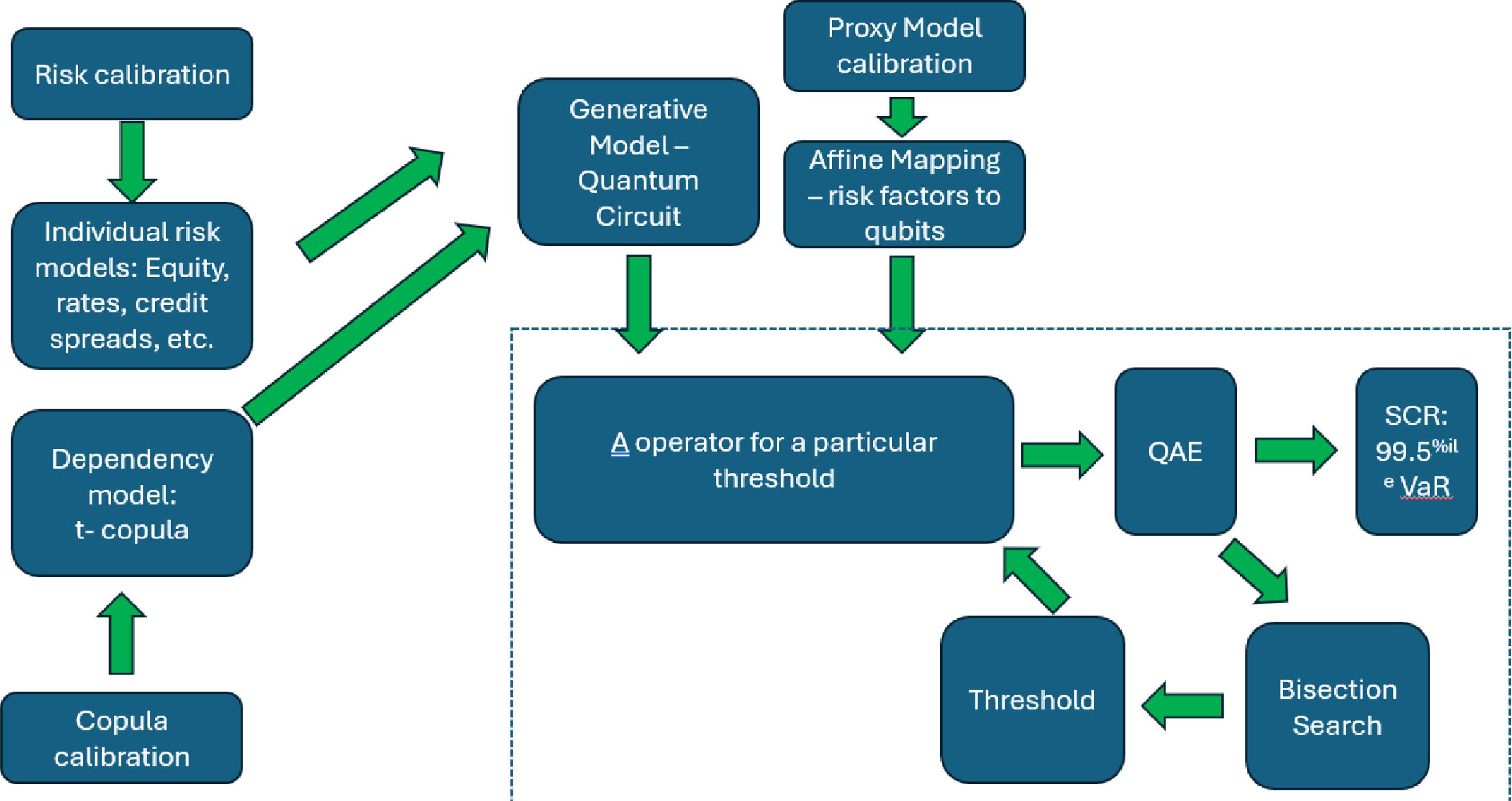
Let’s bring it all together in Figure 16 and see what the end-to-end would look like under this quantum approach. We start in the classical realm with the risk calibrations fitting parametric distributions to historical data for equities, interest rates, credit spreads, inflation etc., and the dependency modelling joining these via the copula proxy model calibration. So far, we have not left the classical realm. Inside this dotted box, we move into the quantum realm, where the risk and dependency structure are mapped to the generative model, which is implemented in a quantum circuit. It replaces our classical scenario generator, encoding our joint risk distribution onto qubits. In parallel, the proxy model is translated into qubit terms as we saw before, essentially rewritten as a function of qubits rather than as a function of risk factors. Inside the staff box we see the A operator, essentially that whole circuit we saw before that flips the state of the final qubit if the loss exceeds a particular threshold. We then query this using QAE for a given threshold. If we find that the amplitude is equal to 0.5%, we stop because that threshold then represents our SCR. Otherwise, we proceed with the bisection search algorithm, which iteratively adjusts the threshold. Then it feeds back, and we keep repeating until we have found 0.5% as our answer for the amplitude, which would then mean that we have found the SCR.

Figure 16.

Bringing it all together!

Now for some sober reflections. Unfortunately, and I say this with a heavy heart, I did not find any measurable computational advantage in running this calculation on a quantum computer. In fact, quite the opposite. The amount of overhead required to prepare the model for quantum execution was staggering. It far exceeds the time needed to run a full SCR calculation on a laptop these days. Let’s discuss why that is.

Figure 17 captures software challenges. The first problem is scale. We have seen before that an arbitrary quantum state requires an exponential number of gates as the number of qubits increases. For 31 risk factors, the generative model alone can have a gate count of 2 to the power of 620. Classical computers cannot even prepare that state. Fortunately, parametric distributions that we tend to use, like the normal and t and so on, have internal structures that can result in more efficient coding, but it is still expensive. We can also look at alternative machine learning-based approaches. The chart on the right of Figure 17 we have seen before. It illustrates how the depth explodes. A more efficient approach would clearly be needed. For instance, one that I discussed in the paper called “Quantum Circuit Born Machines” is a quantum machine learning-inspired approach. But machine learning-based approaches introduce their own layers of training, tuning and validation overhead. I won’t cover them today due to time constraints.

Figure 17.

Software challenges.

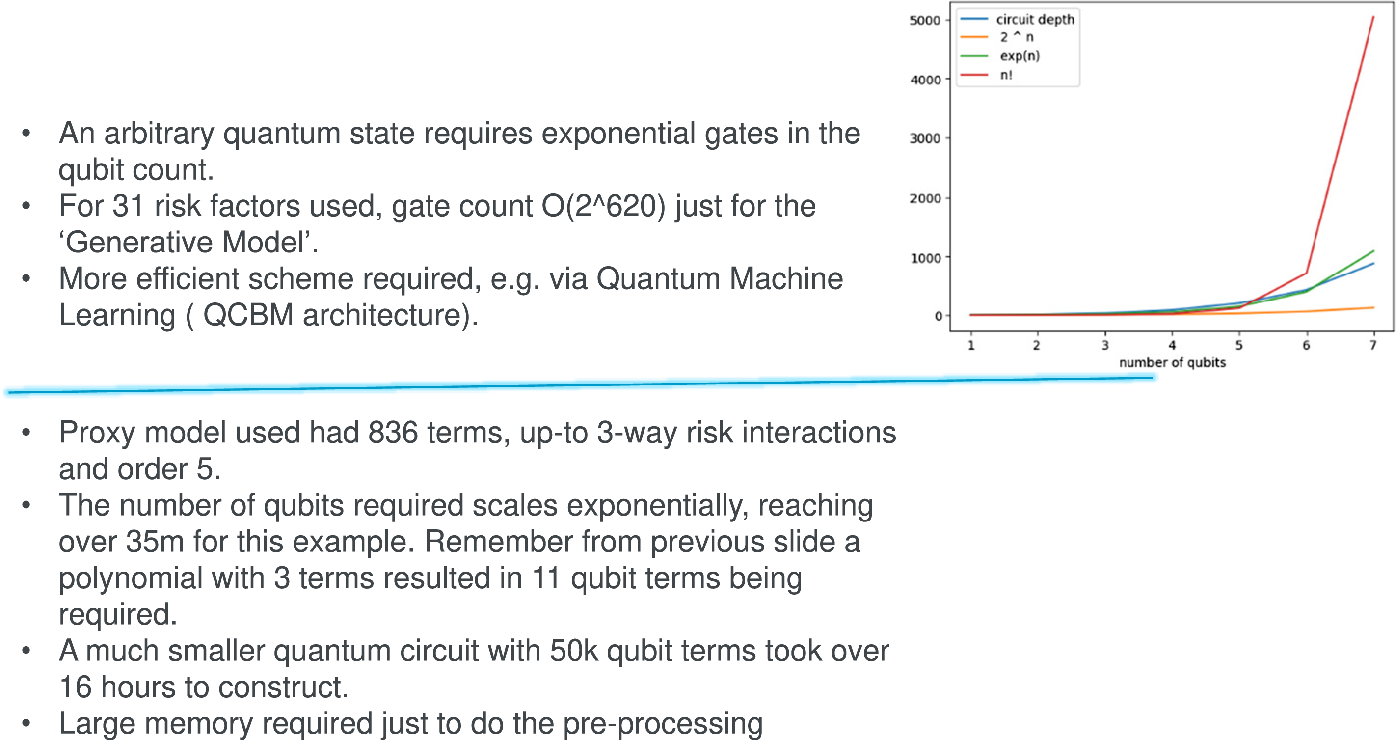
Then we get to the second bottleneck, which is the proxy model itself. I mentioned that the model I used contained 836 terms up to 3-way interactions, and a polynomial order of 5. I mentioned this resulted in the 35 million qubit requirement, and that is before adding all the extra qubits for the weighted sums, the positive and negative editions, the comparators, the thresholds, and the QAE querying itself. The full computational graph is large.

I will briefly cover the hardware challenges as well (Figure 18), which obviously make the picture worse. At the current time we live in what is called a noisy intermediate state quantum (NISQ) era. This means that the qubits that we have today are noisy, unstable and prone to errors. Figure 18 on the left shows a comparison between the theoretical distribution – the simulated distribution – which is what we get from assuming perfect qubits; and then running it on actual quantum hardware. This distribution is what we have seen before, in the dense encoding example. You will see the theoretical and the simulated result are quite close to each other, but the real quantum hardware is a bit different. It is similar, but different.

Figure 18.

Hardware challenges: Noisy intermediate state quantum (NISQ).

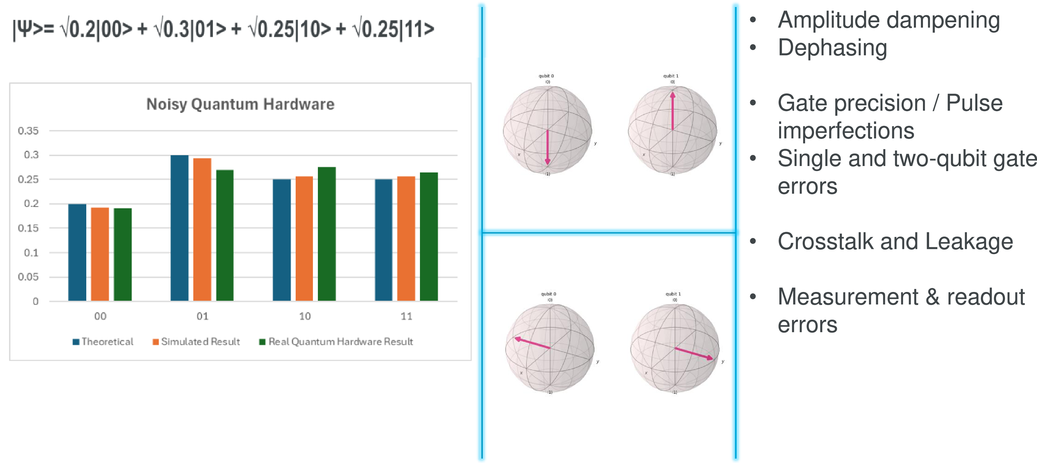
There are broadly four classes of error that contribute to this. The first is what is called dampening and dephasing. Remember our Bloch spheres from earlier? These errors mean that a qubit’s position on that sphere drifts over time. You can think of it like a children’s game of “Telephone.” You tell something to one child and they tell it to another, and after a few passes the message has changed completely. In the same way as time progresses, the qubit can forget part of its state. The second is to do with gate precision and pulse imperfections. Theoretically, amplitudes can take any real value. They can be infinitely precise. But in practice, our control hardware can only manage up to about 3 or 4 significant figures of precision. The gates we apply are not perfect. Every small pulse error nudges the qubit slightly off course. Then there is crosstalk and leakage between them, which means that qubits that should not be interacting sometimes do. We saw what interacting can mean in terms of entanglement earlier in the talk, and leakage would mean that they escape the energy levels, that is, they go outside of the computational basis state, which means that sometimes they are in state 2 or 3 rather than only 0 or 1, which is another practical challenge.

Finally, there are measurement and readout errors. Sometimes, results can be misread. The bottom line is that we need additional qubits just to manage the noise, and the exact overhead can depend on the error correction scheme, but the multipliers are enormous factors of 10, 100 or even 1000 in some cases. My 35 million qubit requirement for a modest but realistic IM can turn into a 35 billion qubit requirement. That is the gap between theory and today’s hardware reality.

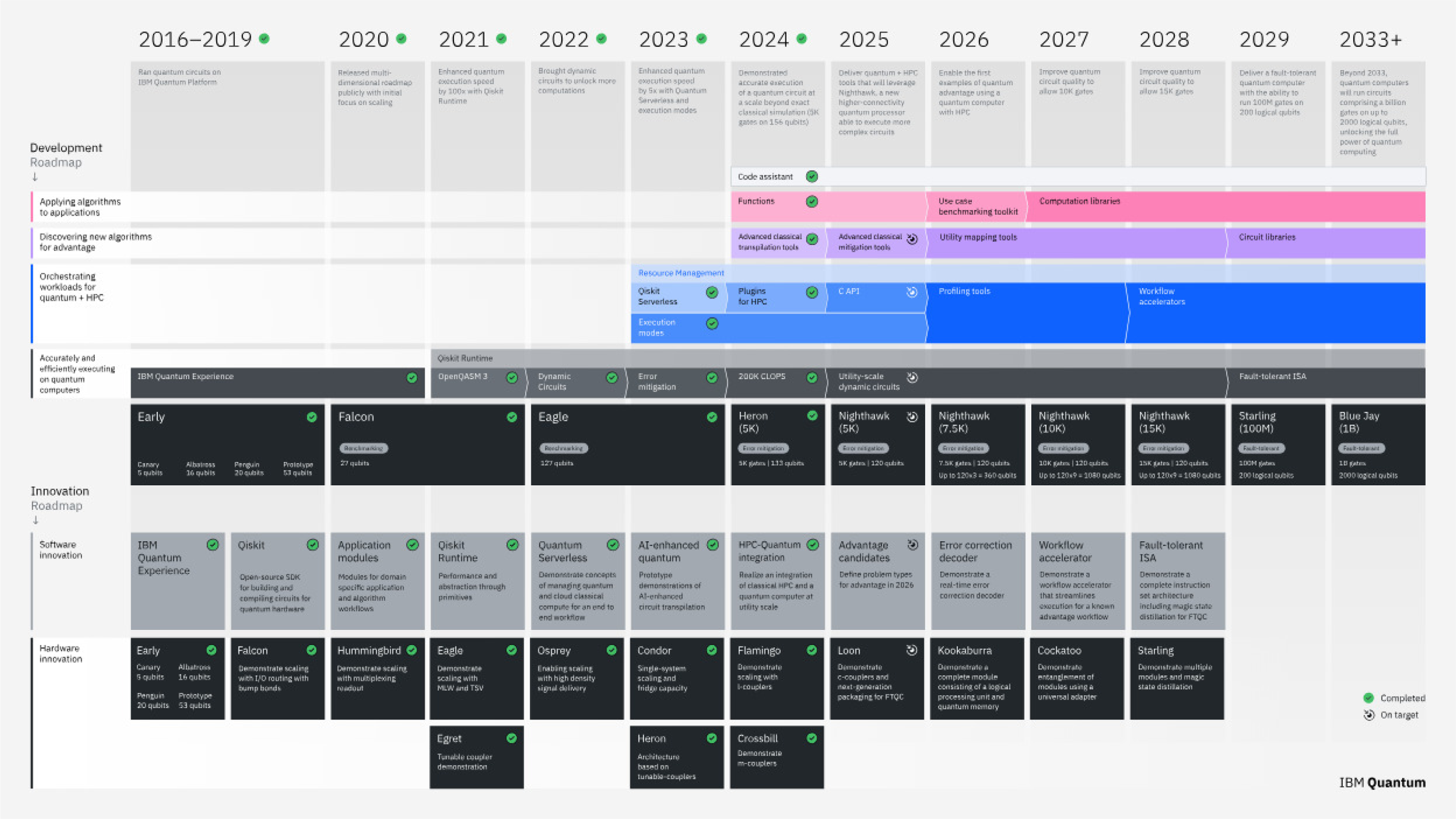
The next era is what we call fault-tolerant quantum computing, which is essentially closing the gap between what we have today versus where we need to get to. This brings us to Figure 19.

Figure 19.

The future.

Remember that quantum computing is advancing at an extraordinary pace, and the momentum, both intellectual and financial, is enormous. Just last month, PsiQuantum raised over 1 billion dollars in private capital – a real milestone for this field. At the same time, governments around the world, including the UK, EU and the US have launched multi-billion-pound national quantum programs. This level of investment, collaboration and belief in the technology is unlike anything we have seen since the early days of artificial intelligence.

On this slide, you can see the IBM quantum roadmap, which I have chosen because it is the ecosystem I have worked most closely with. IBM is what we call a full-stack provider, because they build both the hardware and the software side. They can plan end-to-end progress across the entire stack. You can see the trajectory here, from the early 20- and 100-qubit processors, to the last few years, through to the next generation: Nighthawk, Starling and beyond, eventually targeting fault-tolerant systems with hundreds of thousands of logical qubits by the early 2030s. That is the point at which models like the one I have presented might move from theory to practical implementation.

You might be wondering, why invest the time in learning this technology, especially after seeing that my own use case did not deliver any quantum advantage. That is a perfectly fair question. To me, this project was never about chasing a success story. It was about exploration. What I have learned through this journey is that use cases requiring very precise encoding of the problem, like proxy models where every term and coefficient must be represented explicitly, are probably not where quantum computing will shine first. The circuits become too deep, the error rates are too high, and today’s hardware is just not there. But there is an entirely different class of problems, ones that are much easier to encode and that are naturally much more fault-tolerant. These include combinatorial optimisation problems: problems that are messy, complex and discrete by nature, where quantum computers even today can genuinely help us to search vast solution spaces more efficiently. In fact, the work by Tim Berry and James Sharpe on quantum ALM is a brilliant example. They showed how a particular type of optimisation problem, called a QUBO, which stands for quadratic unconstrained binary optimisation, can be expressed and solved efficiently on a quantum annealer, which is a type of quantum computer specifically designed for optimisation problems. That is just one example. There are many other problems in risk, finance and operation research that might lend themselves naturally to quantum approaches. You can even think about quantum random numbers. Those who play around with finding the right seed for with-profits-cost-of-guarantee calculations might find it useful.

We just have to keep an open mind, stay curious and be willing to experiment. For me, this has been an incredibly rewarding journey coming from a non-computer science background. Concepts like Two’s complement, quantum arithmetic and state-space decomposition were all completely new to me. But with every obstacle I hit, I learned something new, and that ultimately is how progress happens. It reminds me of a quote by Marcus Aurelius, which has stayed with me throughout all the challenges I encountered during this work: ‘Impediment to action advances action, what stands in the way becomes the way.’ Thank you for your attention, and I hope some of you will be inspired to explore your own quantum way from here.

Moderator (starting the Q&A session): Thanks, Muhammad (Amjad). That was a considerable amount of food for thought. Thank you for taking us through that. It is fair to say that while quantum computing at this point may not have any obvious benefit for IMs, there are benefits for optimisation-based problems. That is based on our current use of the way quantum mechanics works, as a theory. There is a question asking about additional sources that you would recommend to build up knowledge in this area from a beginner level.

Mr Amjad: I would recommend just getting started. I mentioned my own journey of reading textbooks. There are quite a few behind me that I can recommend, but there is nothing like getting started. I should say tools like ChatGPT have made experimentation a lot easier compared to how it was in the pre-2023 world. We will be sharing Q&A notes later. I will insert a few textbooks in there for your reference. There are textbooks that are specific to Python that connect quantum computing with Python programming. If you are unfamiliar with both, you can pick up both at the same time, which I can recommend.

Questioner: You mentioned quantum computing reduces the sample complexity. Is that not just a function rather than parallelisation? Is that not just a function of the fact that quantum computing essentially vectorises computations at a much lower level than you would ordinarily do? Rather than vectorising at the bit level, it is not really vectorising when you put into C code or into binary code, but quantum computing really does vectorise at a much lower atomic level rather than at a binary level. It is a different level of abstraction you are looking at, but it is primarily the same mechanics.

Mr Amjad: I would say it is even deeper than vectorisation. With vectorisation you are still working with that bit-by-bit comparison, everything is either 0 or 1. The key insight is here, you can represent multiple states at the same time. What this QAE is doing is exploiting the internal structure. The example I would give is, think about that game Twenty Questions. Think about how many questions you might need to ask someone if they gave you only a “yes” or “no” answer. Now contrast that with someone who gives you a probability distribution every time you ask them, rather than just a simple yes or no. You can exploit the information in that probability distribution to get to the answer quicker than you would be able to with just 0s and 1s.

Questioner: How does the cost of running quantum models compare to using traditional computing? I understand quantum computers need to be cooled down to a very low temperature to reach their steady state.

Mr Amjad: I think it is a lot higher. That is why the business benefit needs to be there. The nice thing is for experimentation. You can create an account with IBM, and they will give you ten minutes of usage for free every month. Similarly, I think D-wave is what James Sharpe and Tim Berry used for their quantum optimisation example. D-wave also gives you a few minutes free every month. If you are just building a proof of concept, you can do it for free. If you are an academic, you can reach out to one of these organisations and get some additional credit from them. If you start deploying it commercially, then it can become costly, which is why the benefit needs to be there from a commercial outcome perspective.

Questioner: One of the challenges of quantum computing in general is that the so-called steady state may change. It is random, essentially. You mentioned that it is essentially perfectly random, that is, we do not understand the cause of the randomness. It cannot be replicated. Isn’t this problematic, even if we could generate the amount of computing power that we would need? Isn’t this problematic from a regulatory point of view? Currently, we always have an error range around SCR because that is just the way we do it. It is the way it is defined. Isn’t this additional level of randomness problematic?

Mr Amjad: It is not additional randomness. It is better-quality randomness. I encourage you to read the article in The Actuary. There is a company called Quantum Dice, which is spun out of Oxford. What they build and make commercially available are these quantum random number generators. They have collaborated with HSBC. The example they have given is of a with-profits type of calculation because they are looking at risk-neutral valuation of contracts with liabilities.

We all know that, at the moment, we rely on pseudo-random number generators that aren’t random. We can see them, and they will produce exactly the same outcome every single time if you use the same seed. With quantum random number generators, there is no way of seeding that randomness. Every time you run the calculation, it will be a different answer. I think that is where your question comes from, that reproducibility and whether the regulators will be concerned. You can flip it. You can say, “Well, because it is better-quality random numbers, you cannot game the random number generator,” whereas a pseudo-random number generator you can game. The example I gave during the presentation of finding the right seed in a with-profits context, you can also play around with the seed for your IM SCR calculation and choose a seed that reduces your SCR by 10 million or whatever, within that funnel of doubt. I would imagine the regulator would be a lot more uncomfortable with the fact that you can game your pseudo-random number generator, compared to something that you cannot even, in theory, game. The challenge is demonstrating to the regulator once and staying on top of it. But they are genuinely better-quality random numbers. They will be much more representative of the risk distribution that you are trying to model.

Questioner: I guess it also opens the possibility of, rather than using the Gaussian or t-copula, which we use purely for practical purposes as they are easy to implement, moving to more neural network-based approaches, or much more sophisticated approaches that possibly better capture systemic risk. A dependency is on the ability to do the computing rather than just a theory.

Mr Amjad: In terms of the dependency modelling, the approach I presented today with the circuit diagrams and so on, and the IBM framework in general, it is called gate-based quantum computing. It is a universal computer, so it can perform any computation that a classical computer can perform. But because it is quantum, it can do more. We are not restricted to Gaussian, or t-copula or Frank or Gumbel or any other copula. We can encode any arbitrary dependency structure. The problem is, when we go into arbitrary territory, it becomes a lot more expensive when we code these arbitrary distributions, as we have seen. The gate count that we require explodes exponentially, which is the reason why, even in the classical realm, we like using parametric distributions because they are easy to simulate from rather than using an empirical distribution every single time.

Questioner: Not so much a question as a thought experiment. Is quantum computing viable to calculate almost-near-time risk moment by moment of a fleet of vehicles that are sharing the data location, breaking. etc., telematically, and the price that they risk for insurance purposes. I guess it is coming down to similar challenges.

Mr Amjad: I would flip this on its head. What is your computational bottleneck in the classical world? Why are you trying to quantise this particular calculation? Insurance companies can be notoriously slow in terms of technology adoption. I often give this example. We have had GPUs for decades now, and they are nowhere near pervasive in the insurance market. There is only a handful of providers here and there who have clocked that there might be an advantage from running certain types of calculations of GPUs. After GPUs you get specialised circuits, Field Programmable Gate Arrays and stuff like that, so quantum computing is way out there. The combinatoric optimisation problems I mentioned are good for quantum computers. There is intractability in those kinds of problems because the state space explodes exponentially. There is internal structure that you can exploit in the quantum realm. That is what makes optimisation a useful use case for quantum computing.

Questioner: How likely do we think that we are to get the required hardware by using quantum computers in the next ten to twenty years? You mention that there is a lot of money going into it, but also a lot of money went into AI. A lot of reports now are saying, ‘Well, there is actually nothing to show, or very little to show for AI’. How likely is all this to materialise into something usable?

Mr Amjad: A few weeks ago, the same team at HSBC demonstrated quantum advantage for a real problem, that is, predicting whether an order is likely to be fulfilled. It is a collaboration between Quantum Dice and HSBC. I think the applications are happening. Going back a few years, one of the German cities used the D-wave quantum annealer to optimise their bus routes. The short answer is, a lot of money is going in and hardware is improving steadily. This timeline that we see on the slide here, already we are approaching the 1000 qubit range over the next couple of years. We have a roadmap for 100,000 as well, presented by IBM, and they are sticking to it. Software advances are also happening. The more people get familiar with this technology and start using it, the more use cases that we will start to uncover.

Moderator: That was all very helpful. Thanks again everybody for joining, and thanks again, Muhammad (Amjad). That was quite a mountainous effort.

Mr Amjad: Thanks Joseph, thanks Brooke for setting this up, and thank you everyone for your attention.

The following additional questions were submitted during the sessional via Chat and answered by the speaker after the sessional.

Questioner: In entanglement, can change in Q1 effect Q0 or is it one way only?

Mr Amjad: This is an excellent question and goes to the heart of the nature and power of quantum entanglement. In classical computing, the information would flow in one direction, if bit A controls bit B, flipping B never changes A. Quantum Entanglement is completely different. Once two qubits are entangled, their states become linked symmetrically. There is no longer a meaningful notion of “Q0 affects Q1” or vice versa. They share a combined state. Measuring the state of one instantly causes the state of the other to jump. In the maximally entangled Bell pair we looked at, the 2 qubits behave as a single, unified quantum system rather than two separate objects.

Questioner: In addition to your paper, which sources would you recommend for building up knowledge in this area from beginner level?

Mr Amjad: There are a number of really good books. I would recommend the following:

1. (1) Quantum Computing with Python and IBM Quantum Experience. This is to help you get started with hands-on examples and Python programming if you haven’t done it before.

2. (2) Dancing with Qubits – Robert S Sutor. This is an accessible introduction to quantum computing and will help you grasp the theory.

3. (3) Quantum Computation and Quantum Information. This is the ultimate textbook for all things quantum computing. It is very dense so it might be worth waiting until you’ve developed some core skills to start this one.

Questioner: How does the cost of running quantum models compare to using traditional computing?

Mr Amjad: The short answer is that classical computing is currently far cheaper, mainly because it has been fully commoditised, while quantum computing is still at a very early stage. Classical hardware has benefited from decades of scaling and cost reduction, whereas quantum machines are still bespoke laboratory systems that require extreme cooling and precision control. This is reflected in cloud costs too: running a quantum circuit is far more expensive, though providers like IBM offer free monthly credits, which is plenty for beginners experimenting with small circuits.

Questioner: Is quantum computing viable to calculate almost-near-time risk (moment by moment) of a fleet of vehicles that are sharing their data (location, acceleration, braking, etc.) telematically? And price that risk for insurance purposes?

Mr Amjad: My counter-question would be: what exactly can we not do with classical computing today for that use case? If the challenge is one of scale, optimisation or dimensionality, then quantum computing could one day accelerate certain sub-problems. Remember, similar to QIMs, the best use case for quantum is not replacing the entire workflow with a quantum version; it is about selectively accelerating the computational bottlenecks where quantum algorithms can genuinely outperform classical ones. So, in a telematics-based, near-real-time pricing set-up, I expect most of the system, the data ingestion, cleaning and inference would remain classical in the same way as in the QIM example, where the calibrations and so on remained classical. Quantum might eventually help behind the scenes, for example in model training or optimisation, but I expect not in the live operational layer.

Questioner: How likely do we think we are to get the required hardware to be using quantum computers within the next 10–20 years?

Mr Amjad: It really depends on the use case. For certain types of optimisation problem, quantum hardware such as annealers, like those from D-Wave, are already capable of providing solutions today. They are not universal quantum computers, but they do offer practical value for specific classes of problems, especially combinatorial optimisation. If the aim is to use true randomness rather than pseudo-random generators, for example, in encryption, sampling or risk modelling, that is also something we can already achieve with today’s hardware through quantum random number generators. These are commercially available and even integrated via Application Programming Interfaces APIs, and they have use cases beyond finance, including cybersecurity and secure communications.

For full fault-tolerant, general-purpose quantum computers, we are likely still a decade or two away, but progress is steady and we’re already seeing intermediate, hybrid approaches emerging where quantum devices complement classical systems rather than replace them.

Questioner: Good point about flipping. My thought is there are a few million vehicles in a typical book of business for very large insurance companies.

Mr Amjad: Once we start talking about millions of vehicles, we’re firmly in the realm of massive parallel inference and data streaming, which classical computing, especially distributed and cloud-based architectures, already handle extremely well. Quantum computing does not scale in that way yet. It does not process millions of data points in parallel like a GPU cluster would. Instead, its power comes from state-space parallelism, the ability to represent many possible states or outcomes simultaneously and manipulate them concurrently through quantum algorithms. So rather than running risk calculations vehicle by vehicle, a more plausible use case would be to encode aggregate relationships or correlations across the fleet, or to optimise higher-level decisions like portfolio-level reinsurance or dynamic pricing strategies. In other words, quantum might eventually help to learn from all of those vehicles rather than track them all individually in real time.