2. Science targets

The CACHMC survey targeted 50 high-mass molecular clumps in the southern Galactic Plane ( $270^\mathrm{o} \lt \ell \lt 20^\mathrm{o}$ , $-1^\mathrm{o} \lt b \lt 1^\mathrm{o}$ ), selected from sources originally identified by the ATLASGAL survey, and subsequently mapped and characterised by the MALT90 and HiGAL surveys (Jackson et al. Reference Jackson2013; Rathborne et al. Reference Rathborne2016; Guzmán et al. Reference Guzmán2015). Five additional high-mass clumps in very early evolutionary stages were added during the survey: AGAL302.486-00.031, AGAL313.576+00.324, AGAL316.752-00.012, AGAL317.429-00.561, and AGAL341.702+00.051. These 70- $\mu$ m dark sources (indicating cold clumps with high optical depth) from the HiGAL database have been observed with ALMA as part of the ASHES project (Sanhueza et al. Reference Sanhueza2019; Li et al. 2022; Sabatini et al. Reference Sabatini2022), and the CACHMC ammonia observations provided supplementary rotational excitation temperature information. An additional four high-mass molecular clumps in later evolutionary stages, as indicated by ammonia (3,3) maser emission, were also added: G23.33-0.30, NGC6334-I, -IV, and -V, each hosting ammonia (3,3) and water masers (Walsh et al. Reference Walsh2011; Kraemer & Jackson, Reference Kraemer and Jackson1995). These additional targets were observed in only two array configurations (750C and 1500C) except the NGC6334 sources (750C only) and G23.33-0.30 (all configurations). Finally, IC 443 was included as a candidate ammonia (3,3) maser site (McEwen et al. Reference McEwen, Pihlström and Sjouwerman2016); it was observed in the 750C array configuration only, but no (3,3) maser emission was detected.

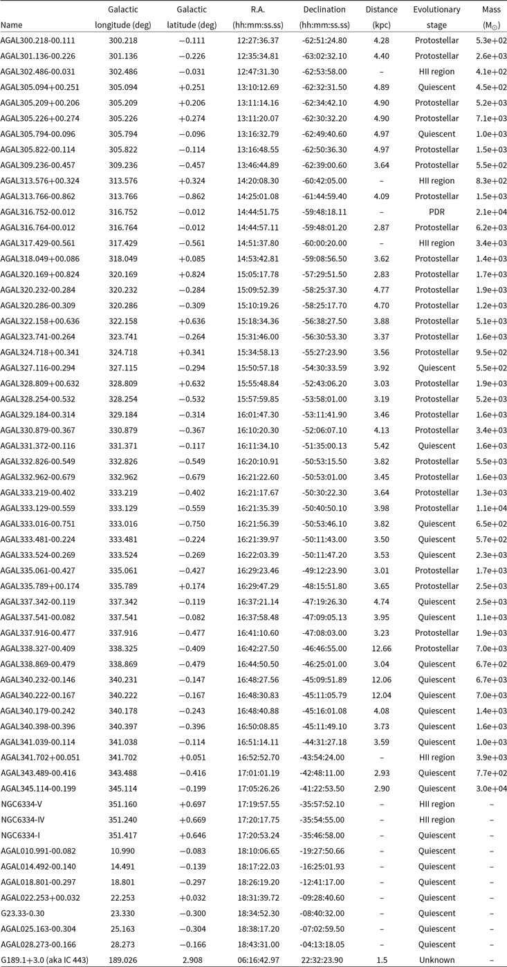
The mid-IR images from the GLIMPSE (Benjamin, Churchwell, & Babler Reference Benjamin, Churchwell and Babler2003; Churchwell et al. Reference Churchwell2009) and MIPSGAL (Carey et al. Reference Carey2009) surveys can be used to characterise the clump’s evolutionary stage (Jackson et al. Reference Jackson2013). Of the 60 targets included here, 25 are classified as ‘quiescent’ and 27 as ‘protostellar’ clumps. These young clumps are promising locations at which to observe nascent massive star formation in its earliest phases. Of the remaining sources, 6 are HII regions and one (AGAL316.752-00.012) is a PDR; the evolutionary stage of IC 443 is unknown. Details of the observed sources are given in Table 1.

Table 1.

List of observed sources and targeted coordinates. Distances, where available, are taken from Whitaker et al. (Reference Whitaker2018) except that for G189.1+3.0 (also known as IC 443), taken from McEwen et al. (Reference McEwen, Pihlström and Sjouwerman2016).

Table 2.

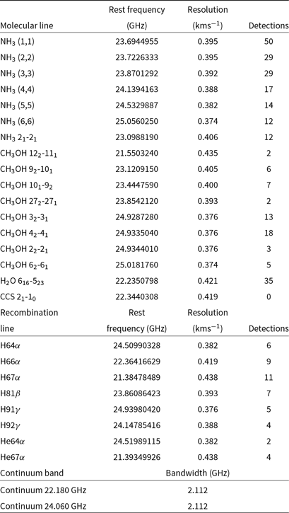
Summary of molecular and recombination lines observed, and central frequency of the 2-GHz-wide broadband continuum bands. Rest frequencies, obtained from the Splatalogue (https://splatalogue.online) are from Pickett et al. Reference Pickett1998, with the exception of the CCS $2_1$ - $1_0$ line which is from Müller et al. Reference Müller, Schlöder, Stutzki and Winnewisser2005). Detections, at the target coordinates, are based on an SNR of 5; see Section 4 for data reduction details.

3. Observations

To carry out the survey, observations were made using the Australia Telescope Compact ArrayFootnote ^a (ATCA) in the southern winter semesters (April to September) from 2017 to 2020. A total of 84 observing sessions were completed. Observations between 21.550 and 25.057 GHz were made using the zoom-band mode of the Compact Array Broadband Backend (CABB; Wilson et al. Reference Wilson2011), with 64-MHz-wide bands and 32-kHz channels. Two 2-GHz-wide continuum bands were also observed. The zoom bands were chosen to cover the primary molecular emission lines of interest: the first six metastable inversion transitions of ammonia, a selection of methanol lines between 23 and 25 GHz, the 23.3-GHz thioxoethenylidene (CCS) transition, the masing water line at 22.2350798 GHz and the H67 $\alpha$ recombination line. The resulting spectral resolution was approximately 0.4 km/s; precise parameters for each observed line are given in Table 2.

In addition to the targeted lines, other spectral lines were observed serendipitously (these included additional ammonia and methanol lines as well as other recombination lines). Details of the full set of observed (and reduced) spectral lines are shown in Table 2: in total, there were 17 molecular emission lines and six hydrogen and two helium recombination lines.

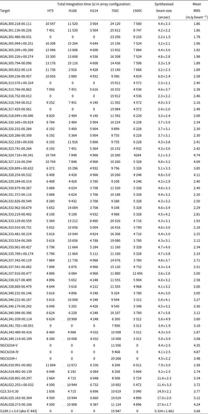
The observations were repeated using five interferometer array configurations: H75, H168, H214, 750C, and 1500C. The configuration names reflect the shortest baseline (in metres) between the array’s antennas; the long-baseline data from antenna CA06 (minimum 3 000-m baseline) was included in the data reduction. The total integration times in each array configuration for the science targets are given in Table 3, along with the synthesised beam sizes (generally approximately 4.5 by 3.0 arcsec) and the RMS noise levels (averaged over all data cubes for each target, typically around 2.5 mJy/beam).

We used standard calibration sources for bandpass, flux, and phase calibration. The quasar 1253-055 was generally used for bandpass calibration, with the BL Lac object PKS 0537-441 used for early-rising sources; the bandpass calibrator was observed once per day. Flux calibration was performed using the quasar 1934-638, also observed once per day. Phase calibrators were selected from the ATCA Calibrator Database for each science target; in most cases the calibrator was shared by multiple close targets. Phase calibrators were chosen which were bright in the 15-mm band and preferably less than 5 degrees away; compromises were resolved in favour of brightness and at the expense of distance from the target. The phase calibrators were observed every 5–15 min, depending on the prevailing atmospheric conditions and the number of targets sharing the calibrator. Overall, the weather throughout the survey was very favourable, with generally dry atmospheric conditions and low to moderate wind speeds.

4. Data reduction

The observations resulted in approximately 5 TB of raw data, which was processed using the Miriad software suite (Sault, Teuben, & Wright Reference Sault, Teuben and Wright1995), following the usual steps for radio-interferometry data reduction. The data were split into individual visibility files, each containing data from a single zoom band for a single source (whether calibrator or science target).

Flagging was performed on the visibility data, removing edge channels (first and last channel of each band) and spuriously high-amplitude visibilities (above 1 000 Jy for all zoom bands except that containing the masing $\mathrm{H}_2\mathrm{O}$ line, for which the threshold was 100 000 Jy). RFI-affected channels were removed, followed by manual inspection of the visibility time-series to remove observations made during periods of high atmospheric instability (identified by particularly noisy or rapidly varying phase measurements), guided by the observing logs.

Bandpass and flux solutions were calculated and applied to each calibration source, and phase correction solutions then calculated. Flux calibrator observations are not available for five observing sessions (2017-07-12, 2017-07-16, 2017-09-09, 2017-09-11, 2018-08-29): on these days the flux calibration solution from the previous day (next day for 2017-07-16) was used. The calibrator solutions were then applied to the science sources.

The calibrated data from all observing sessions was then combined, and channel frequencies converted to velocities using the rest frequencies given in Table 2. Baseline continuum emission was subtracted, and a Fourier transformation performed to produce ‘dirty’ data cubes for each science source, for each spectral line or continuum band. A 1-arcsec pixel size was chosen, in comparison with typical beam sizes of around 3 arcsec, and 512-pixel square images were produced for each spectral channel, large enough to extract a 3-arcmin square region in Galactic coordinates. The FWHM primary beam of the ATCA at these frequencies is $\sim$ 2 arcmin. The channel images were then concatenated to form ( $\ell$ ,b,v) data cubes.

Cleaning was carried out using Miriad’s two-threshold clean function on the central 50% of the image (linear, i.e. 50% of each spatial dimension) using 100 iterations; other settings were the phat parameter of 0.1, gain parameter of 0.1 and two cutoff thresholds of 5 and 1 times the dirty image RMS, as measured using imstat (restricted to emission-free channels). The images were then converted to Galactic coordinates, trimmed to 3-arcmin square regions, and moment 0 (integrated intensity), moment 1 (flux weighted velocity) and moment 2 (velocity dispersion) maps derived. The spectrum at the central (target) position of each cube was also extracted for reference. Finally, the maps and data cubes were converted to FITS files.

Of the 60 sources observed, 50 were detected in the ammonia (1,1) line, 12 in all ammonia lines up to (6,6), and 18 in at least 1 methanol line. Line detection counts, using a SNR threshold of 5, for the central target locations, are given in Table 2. Radio continuum emission was observed within the field of 44 targets.

5. Derived physical properties

5.1. Model of ammonia emission

A model containing five Gaussian hyperfine line components was fitted to the ammonia (1,1) and (2,2) transition spectra, for all pixels in each map, after spatial smoothing was performed by averaging the emission over square regions 5 pixels across. The model attempts to fit the nuclear quadrupole hyperfine structure of the $\mathrm{NH}_3$ lines (Ho & Townes Reference Ho and Townes1983); it does not take into account the additional, smaller, magnetic hyperfine splitting. Since the line widths are in general much larger than this smaller splitting, modelling only the five nuclear quadrupole hyperfine lines is adequate. The model contained seven parameters: the velocity of the main hyperfine component ( $\mathrm{V}_\mathrm{LSR}$ ), the full-width half-maximum amplitude line width (FWHM; common to all components) and five amplitude parameters, one for each hyperfine component, fitted independently. The satellite hyperfine component spacings are given in Table 4. Initial values of the amplitudes were 0.1 Jy/beam for the main component and 0.05 Jy/beam for the satellite components and 5 km/s for the FWHM. The initial value of the $\mathrm{V}_\mathrm{LSR}$ was taken from the ammonia emission as follows.

Table 3.

List of integration times, in seconds, by telescope array configuration. The array configuration names (H75, for example) reflect the length of the shortest baseline in metres. The ‘mean RMS’ is provided as representative of the noise in the data cubes, calculated as the mean of the RMS for each target, averaged over each data cube and over all spectral lines.

Table 4.

Velocity of ammonia hyperfine components, relative to the main component, used in the 5-component hyperfine model.

The ratio of the main component amplitude to the satellite component amplitude for the ammonia (2,2) line is intrinsically larger than for the (1,1) line, due to the components’ quantum statistical weights, and the (2,2) emission was readily detected for most sources. In comparison, some sources exhibited optically thick ammonia (1,1) emission, with the main component amplitude comparable to (or sometimes even lower than) the satellite component amplitudes. Thus, the velocity of the peak ammonia (2,2) emission was used as the initial estimate of $\mathrm{V}_\mathrm{LSR}$ , where detected; otherwise, the velocity of the peak ammonia (1,1) emission was used.

Fitting was carried out by the curve_fit routine from the scipy.optimize library in Python, using the TRF (‘Trust Region Reflective’) algorithm. The fitted model parameters were then used to estimate the optical depth and rotational excitation temperature across each map. In addition, the model was fitted to the ammonia (3,3) emission in order to estimate the optical depth of this transition.

5.2. Optical depth

The rotational excitation temperature and optical depth were calculated from the fitted hyperfine parameters for the ammonia (1,1) and (2,2) transitions, following Mangum & Shirley (Reference Mangum and Shirley2015). Optical depth, $\tau$ , is estimated from the relative brightness of the satellite hyperfine transitions to the main component and cannot be calculated analytically. It was therefore estimated numerically from all four satellite hyperfine components simultaneously (using the Levenberg–Marquardt algorithm to minimise the sum-of-squares error between the data and the model); an initial value of $\tau = 1.0$ was used.

Table 5.

Positions of masers identified in the CACHMC survey. Each maser can be found in the data cube referred to in the column ‘Map name’. Galactic longitude and latitude are given in degrees, velocities in km/s and maximum intensity in mJy. These sources were identified as masers on the basis of their narrow line width, brightness, and point-source-like nature. (c) candidate maser: identification as a maser is not certain. Rest frequencies for the lines are given in Table 2.

Let $T_R(m)$ and $T_R(s)$ be the measured intensity of the main and satellite hyperfine components, respectively, and $\tau_{(1,1)}$ the optical depth of the main component of the ammonia (1,1) emission. We obtained $\tau_{(1,1)}$ by solving

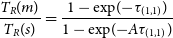(1) \begin{align} \frac{T_R(m)}{T_R(s)} = \frac{1-\exp\!({-}\tau_{(1,1)})}{1-\exp\!({-}A\tau_{(1,1)})} \end{align}

simultaneously for the inner ( $A = \frac{5}{18}$ ) and outer ( $A = \frac{2}{9}$ ) hyperfine components; the sum-of-squares error for the four components was minimised to obtain the best fit. The published data set (see Section 8) also contains estimated optical depths for ammonia (2,2) ( $A_\mathrm{inner} = 0.0651$ , $A_\mathrm{outer} = 0.0628$ ) and (3,3) ( $A_\mathrm{inner} = 0.03$ , $A_\mathrm{outer} = 0.0296$ ).

5.3. Rotational excitation temperature

Using $\tau_{(1,1)}$ and the FWHM for the (1,1) and (2,2) transitions, $\Delta v_{(1,1)}$ and $\Delta v_{(2,2)}$ , respectively, the excitation temperature was then calculated (Mangum & Shirley Reference Mangum and Shirley2015) using the brightness temperature of the $\mathrm{NH}_3$ (1,1) and (2,2) transitions, $T_{B,(1,1)}$ and $T_{B,(2,2)}$ , respectively, as

(2) \begin{align} & T_{ex}((2,2);\ (1,1)) \nonumber \\ & = \frac{-41.5} {\ln\left[ -\frac{0.283 \Delta v_{(2,2)}}{\tau_{(1,1)}\Delta v_{(1,1)}} \ln\left( 1- \frac{T_{B,(2,2)}}{T_{B,(1,1)}} (1-\exp\!{[}{-}\tau_{(1,1)})] ) \right) \right] }. \end{align}

The statistical errors for the ammonia (1,1), (2,2), and (3,3) optical depths and for the rotational excitation temperature were computed using a bootstrapping Monte Carlo approach. For each model parameter, a random value was drawn 1 000 times from a Gaussian distribution with mean equal to the optimal parameter value and variance equal to the variance of the parameter estimates, as reported by the fitting routine. The optical depth and excitation temperature were then calculated using each set of random parameters, and the mean and variance of the resulting distributions calculated to estimate the uncertainty of these derived values. These values are included in the data release; variances for the optical depth are typically below 0.1 and below 2 for the excitation temperature.

The rotational excitation temperatures calculated from the CACHMC data at the target locations have a mean of 19.42 and range of 11.37–28.38. These values in agreement with previously reported data: for example, Urquhart et al. (Reference Urquhart2011) reports a mean of 19.3 and range of 10.2–39.0 for a large sample of similar massive star-forming regions. Line widths are also in accord to those previously reported, with a mean of 3.03 (range 0.57–10.43) in the CACHMC data, compared with 1.9 (range 0.2–7.8) (Urquhart et al. Reference Urquhart2011.)

Figure 1.

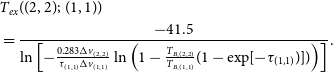
Spectra of selected masers detected during the survey. (a) AGAL337.916-00.477 (‘Nessie A’) $\mathrm{NH}_3$ (3,3) maser; (b) NGC6334-I $\mathrm{NH}_3$ (6,6) maser, at 8.926 km/s (indicated by the red arrow: other emission is thermal); (c) AGAL305.209+00.206 $\mathrm{CH}_3\mathrm{OH}$ 10-9 maser; (d) AGAL335.789+00.174 $\mathrm{H}_2\mathrm{O}$ $6_{16}$ - $5_{23}$ maser. Channel widths are approximately 0.4 ms $^{-1}$ . The masers can be found in these targets’ data cubes; coordinates of the maser sites are given in Table 5.

6. Masers

Many of the observed spectral bands included molecular line transitions capable of masing. These include ammonia (3,3), ammonia (6,6), water $6_{16}$ - $5_{23}$ and multiple methanol transition lines. The lines, locations, velocities, and peak flux of detected masers and maser candidates are given in Table 5. These sources were identified as masers on the basis of their narrow line width, brightness and point-source-like nature. Examples of maser spectra observed are shown in Fig. 1.

Figure 2.

A map of the 22.180-GHz continuum emission for AGAL337.916-00.477 (‘Nessie A’); contours show the moment 0 ammonia (1,1) emission (contour values are 1, 50, 200, and 500 mJy/beam).

Figure 3.

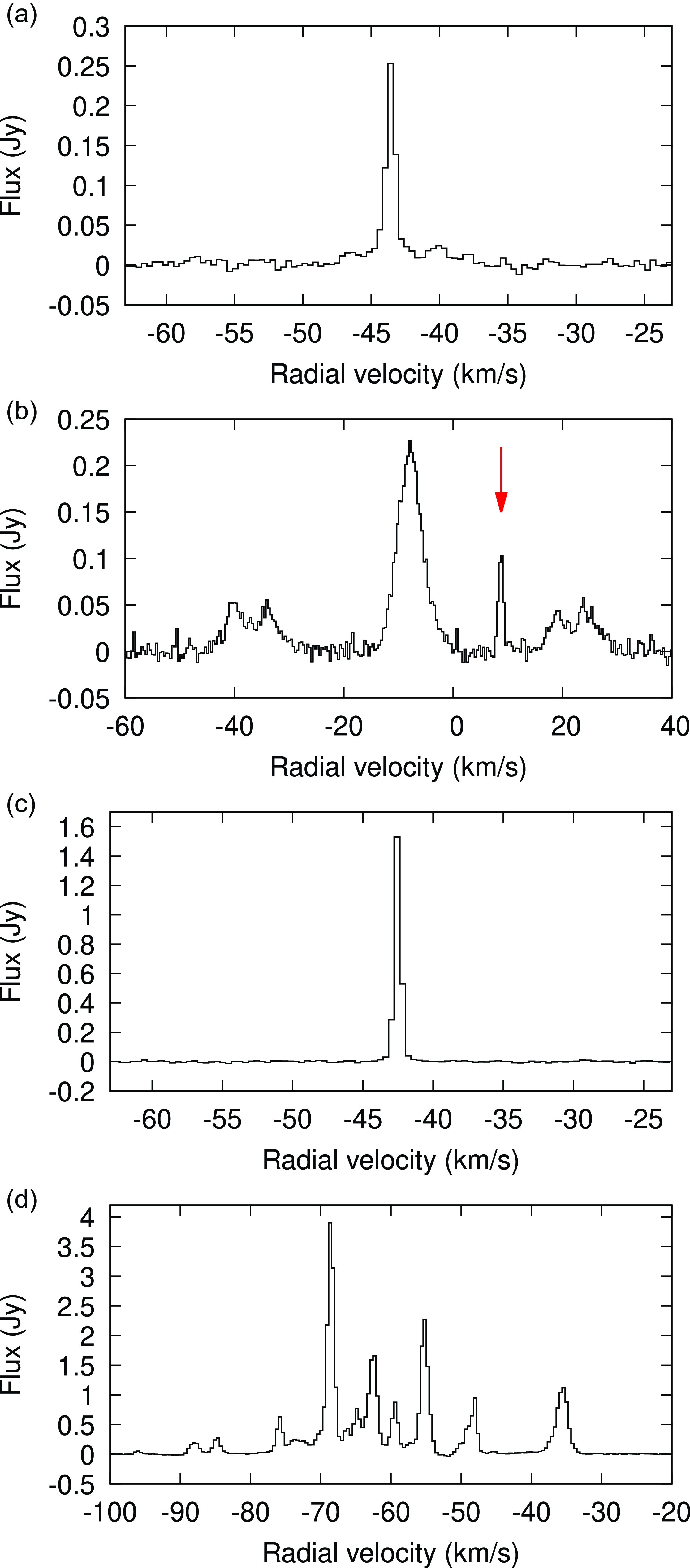
Maps showing derived physical properties of AGAL337.916-00.477 (‘Nessie A’): (a) full-width half-maximum line width, (b) optical depth, and (c) excitation temperature, $T_{ex}$ (with $\mathrm{NH}_3$ (1,1) contours as in Fig. 2 included for reference). At the peak of ammonia emission, near (337.915 $^\mathrm{o}$ , -0.478 $^\mathrm{o}$ ), the derived temperature becomes non-physical, since the $\mathrm{NH}_3$ (2,2) emission is stronger than (1,1): the assumption of LTE is broken, assuming a single gas component. The beam, $3.6\times 2.8$ arcsec across, is shown as a small ellipse in the lower left-hand corner of each map.

Figure 4.

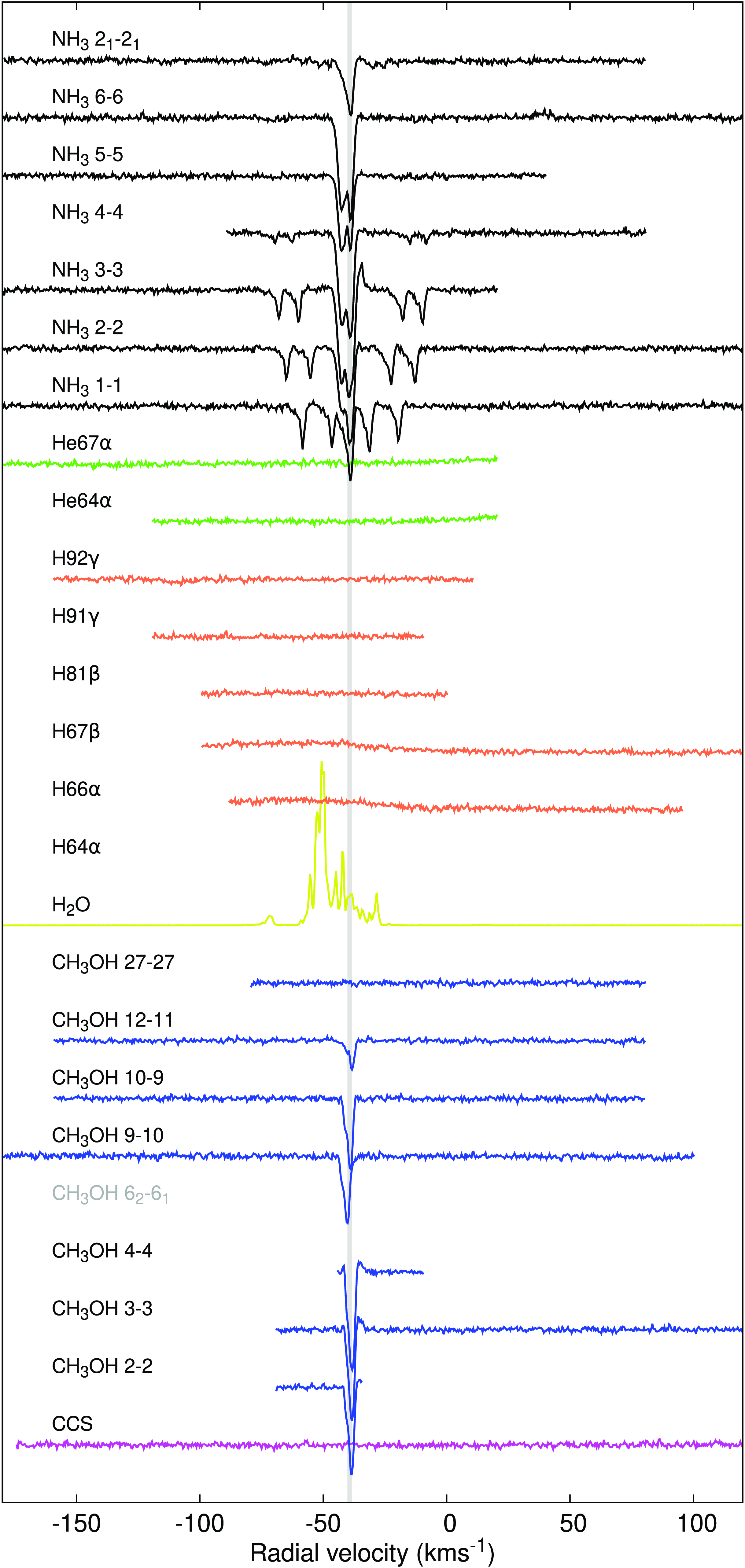
A combined plot of transition lines at the target position of AGAL337.916-00.477 (‘Nessie A’). Lines are all shown at the same scale (except for the masing $\mathrm{H}_2\mathrm{O}$ line, shown in yellow, whose emission has been down-scaled by 100X) and have been vertically offset from each other by 0.2 Jy/beam. The data is aligned to radial velocity: a vertical bar has been added at the target’s systemic velocity ( $-39.58$ km/s) to aid visual interpretation. The plotted velocity range of the data reflects the number of channels in each transition line’s data cube, which varies. Note that there is no $\mathrm{CH}_3\mathrm{OH}$ $6_2$ - $6_1$ data for this target: it lies outside the velocity limits of the receiver band for this line. Line colours distinguish the different molecules and atoms.

Figure 5.

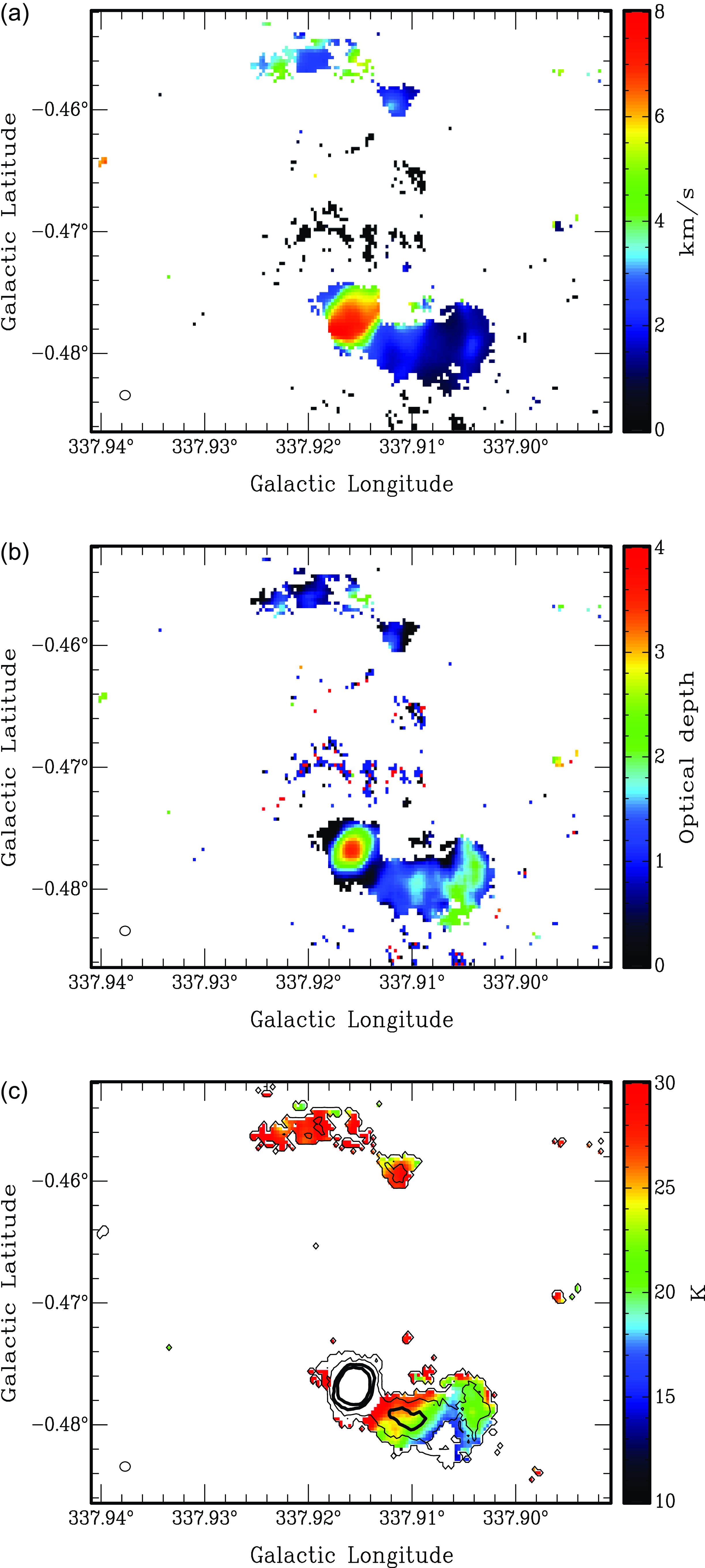
A map of the $\mathrm{NH}_3$ (1,1) hyperfine anomaly, showing the ratio of the left inner hyperfine component to the right inner hyperfine component, for AGAL337.916-00.477 (‘Nessie A’). The relative velocities of the components are given in Table 4.

Multiple ammonia masers were observed, including two previously unknown ammonia (3,3) masers in the ‘Nessie Nebula’ (Jackson et al. Reference Jackson, Finn, Chambers, Rathborne and Simon2010), near the positions of the dense clumps AGAL337.916-00.477 (‘Nessie A’, Fig. 1(a)) and AGAL338.327-00.409 (‘Nessie C’). A previously known ammonia (6,6) maser in NGC6334-I was confirmed (Beuther et al. 2007, Fig. 1(b)).

Masers were observed in 6 methanol transition lines. The survey detected Type I methanol masers in the 2-2, 3-3, 4-4, 6-6, and 10-9 transitions and Type II methanol masers in the $9_{2}$ - $10_{1}$ transition.

The methanol 10-9 transition is a very rare masing line, first detected in 2011 (Voronkov et al. Reference Voronkov2011). We observed a maser at this frequency near AGAL305.209+00.206 (Fig. 1(c)), and three candidate maser sites near AGAL330.879-00.367. Type II methanol masers, in the rare $\mathrm{CH}_3\mathrm{OH}$ $9_{2}$ - $10_{1}$ masing line at 23.121 GHz, were detected near NGC6334-I and NGC6334-V; the former has been observed previously (Cragg et al. Reference Cragg2004).

The $\mathrm{H}_2\mathrm{O}$ 22.2350798-GHz spectral line is a common maser transition that indicates shocks associated with star-forming regions. Water masers were detected towards 43 of the 60 observed clumps, often slightly displaced from the ammonia emission peaks. Almost all of these exhibited multiple velocity components: one of the sites near AGAL335.789+00.174 contains at least 12 distinct peaks at different velocities (Fig. 1(d)).

The data release contains the spectra of the detected masers and candidates and maps showing the position of the masers relative to the ammonia (1,1) emission for each target.

7. Data examples

7.2. Absorption lines

The survey revealed interesting absorption features against the free-free continuum emission from a central H II region. Such absorption was most prominent at the central positions of AGAL301.136-00.226, AGAL328.809+00.632, and AGAL332.826-00.549, with strong absorption in all ammonia lines. 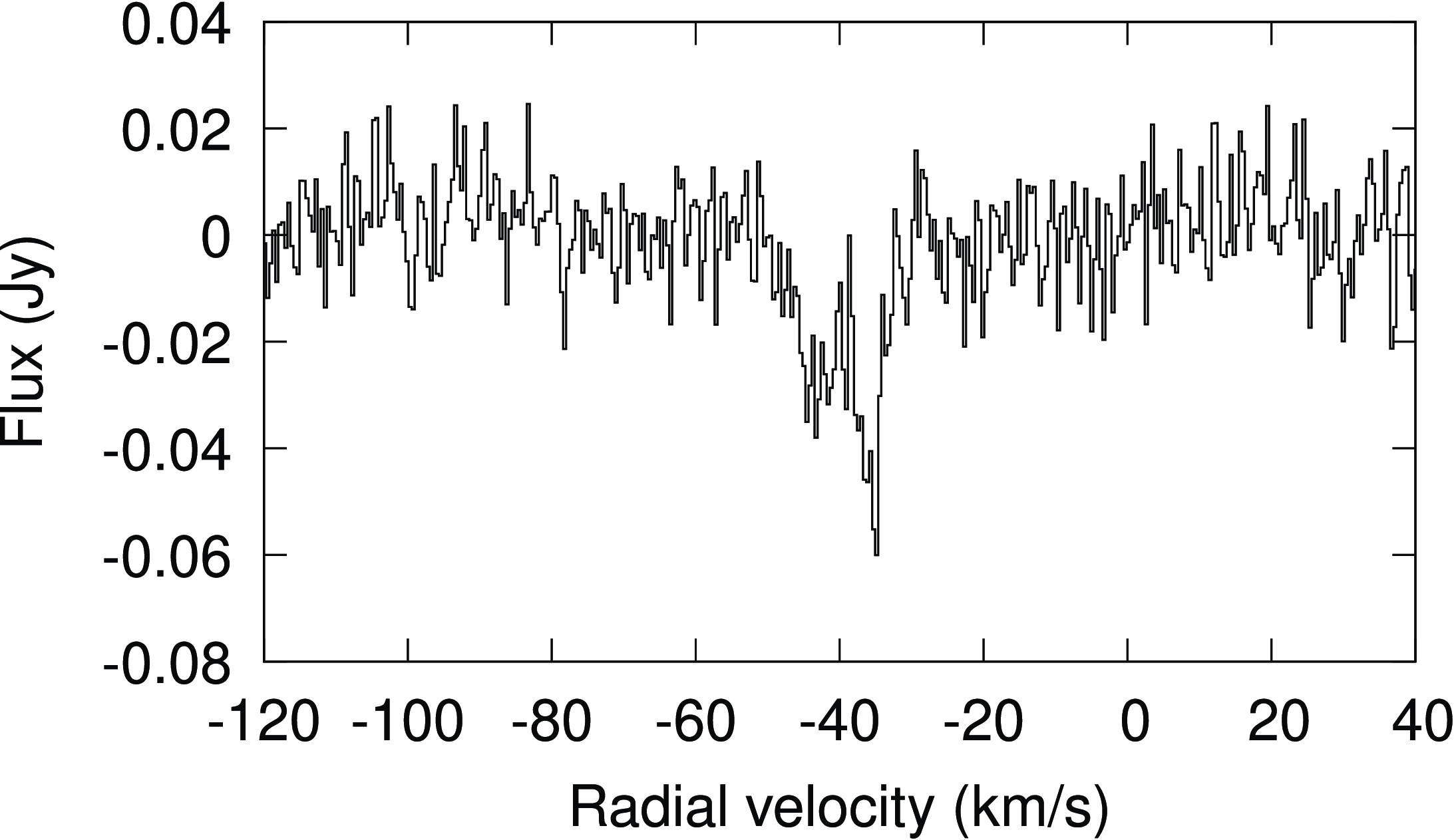Absorption features were prominent at off-centre positions for AGAL320.232-00.284, AGAL322.158+00.636 and NGC6334-IV, but only for the $\mathrm{NH}_3$ (1,1) and (2,2) lines. The central spectra for AGAL301.136-00.226 are shown in Fig. 6, where absorption in all ammonia and most methanol lines can be seen. In addition, an unexpected absorption feature in the 22.23 GHz water line was observed for AGAL328.809+00.632, at the same radial velocity as the ammonia absorption features. This feature is shown in Fig. 7.

Figure 6.

A combined plot of transition lines for AGAL301.136-00.226. Strong absorption can be seen in the ammonia and methanol spectral bands, along with evidence of emission at the edge of the $\mathrm{CH}_3\mathrm{OH}$ 3-3 and 4-4 absorption features. The target exhibits ammonia emission close to the absorption velocity. Lines are all shown at the same scale (except for the masing $\mathrm{H}_2\mathrm{O}$ line, whose emission has been down-scaled by 100X) and have been vertically offset from each other by 0.2 Jy/beam. The data is aligned to radial velocity: a vertical bar has been added at the target’s systemic velocity ( $-39.2850$ kms $^{-1}$ ) to aid visual interpretation. The plotted velocity range of the data reflects the number of channels in each transition line’s data cube, which varies. Note that there is no $\mathrm{CH}_3\mathrm{OH}$ $6_2$ - $6_1$ data for this target: they lie outside the velocity limits of the receiver band for this line. Line colours distinguish the different molecules and atoms.

Figure 7.

Absorption feature in the 22-GHz water spectral band for AGAL328.809+00.632; it is almost central to the map, lying 1–2 arcsec away from the position of maximum ammonia absorption, and the radial velocity of this absorption feature matches the radial velocity of emission and absorption in other spectral lines.

8. Data release

The CACHMC dataFootnote ^b (https://doi.org/10.25919/74nw-9r95) is available to download from the CSIRO’s Data Access Portal, at https://data.csiro.au/collection/csiro:59354. The project website at https://cachmc.space provides galleries of moment maps and central spectra.

The files included in the data release are arranged into five directories, each (except masers/) containing a subdirectory for each science target:

• • data/: data cubes and derived moment maps, RMS maps and central spectra;

• • hfa/: ammonia (1,1) hyperfine anomaly maps; and

• • ircontext/: mid-infrared context images overlaid with ammonia (1,1) emission contours;

• • masers/: catalogue and spectra of detected masers.

• • temperature/: derived temperature and optical depth maps;

In addition to the observations detailed in Section 3, continuum data was collected at 5.5 GHz and 9.0 GHz for 15 targets exhibiting strong 22- and 24 GHz continuum emission; these observations were undertaken during weather unsuitable for the usual, higher frequency, observations. The raw data for these observations (as well as all other CACHMC raw data) are available in CSIRO’s Australia Telescope Online ArchiveFootnote ^c (ATOA) with the project code ‘C3152’.

Details of the directory structure and the included files in the data release are given in Appendix 9.

9. Summary

The CACHMC Legacy Survey was carried out on the ATCA over four winter observing seasons and successfully observed 60 potential sites of future high-mass star formation. High signal-to-noise ratio data for ammonia (J,K) = (1,1) through (6,6) transitions were collected, and 24 ammonia (3,3) masers identified, along with 19 spectral lines (including $\mathrm{H}_2\mathrm{O}$ and methanol masing lines). Continuum emission was measured at 22 and 24 GHz. Ammonia HFAs were observed and found to be common, as previous studies have shown, but also occurring in spatially extended molecular gas.

Data products from the survey have been prepared and include FITS data cubes for the observed spectral lines, along with central spectra and moment 0, 1, and 2 maps for the 60 targets. These observations are now available to characterise the turbulent structure within the target clumps and to measure the locations, temperatures, masses, temporal sequence and kinematics of their individual star-forming cores.