


Impact Statement
In most microfluidic applications, the fluids involved are biological fluids, chemicals or mixtures of solid samples and reagents, which often exhibit nonlinear response to applied stress. Mixing such types of fluids is quite difficult, especially because of the laminar flow regime and high viscosity involved. The numerical investigations conducted in this work shed light on the flow physics and magnetohydrodynamic mixing of such non-Newtonian fluids. The results presented in this study will be greatly useful for the design and fabrication of microfluidic devices dedicated to magnetohydrodynamic flow control, micromixing and microreaction, where the fluids involved are non-Newtonian in nature and compatible with electromagnetic forces. The proposed device requires no external pumping mechanism and the compact design of the micromixer offers ease of integration with different lab-on-chip systems in chemical and biomedical analysis.
1. Introduction
Microfluidic technology has witnessed tremendous growth in the last couple of decades due to its indispensible applications in the field of biomedical analysis (Yang et al. Reference Yang, Chen, Tang, Zong and Jiang2020), nanomaterial synthesis (Li et al. Reference Li, Li and Wang2017), chemical synthesis (Elvira et al. Reference Elvira, i Solvas, Wootton and deMello2013), micro-analysis (Noviana et al. Reference Noviana, Ozer, Carrell, Link, McMahon, Jang and Henry2021) etc. Flow manipulation is often a crucial aspect in such microfluidic devices and various methodologies have been developed over the years for the same. Depending on the area of application and physical properties of the fluids involved, there are various techniques of fluid actuation – pressure driven actuation, electrohydrodynamic actuation (Peng et al. Reference Peng, Li, Yang, Ma and Mao2023), acoustic actuation (Gao et al. Reference Gao, Wu, Lin, Zhao and Xu2020) and magnetohydrodynamic actuation (Derakhshan & Yazdani Reference Derakhshan and Yazdani2016).
In the context of micromixing, there are two broad categories – active and passive micromixers (Bayareh et al. Reference Bayareh, Ashani and Usefian2020). Passive micromixers do not rely on any external energy input (Juraeva & Kang Reference Juraeva and Kang2020; Tripathi, Patowari & Pati Reference Tripathi, Patowari and Pati2021) while active micromixers employ external agents like electric (Kumar et al. Reference Kumar, Manna, Sarkar and Biswas2024), magnetic (Jeon et al. Reference Jeon, Massoudi and Kim2017), acoustic forces (Barman & Bandopadhyay Reference Barman and Bandopadhyay2023) etc., for efficient mixing of fluids. Application of electromagnetic forces to drive conducting fluids in microchannels has gained much attention in recent years. Ionic solutions or electrolytes, composed of positive and negative ions, are subjected to Lorentz forces to generate flow, termed magnetohydrodynamic (MHD) flow. When such fluids are subjected to both electric and magnetic fields, Lorentz forces are exerted on the ions (Bau et al. Reference Bau, Zhong and Yi2001) in a direction perpendicular to both the electric and magnetic fields. The direction of the force can be easily varied by changing the direction of the electric or magnetic field and applying different electrode combinations and magnets.
Studies have shown that MHD devices have the potential to serve not only as pumping devices (Jang and Lee Reference Jang and Lee2000) but also as micromixers (Jeon et al. Reference Jeon, Massoudi and Kim2017) and in some cases as both (Kang & Choi Reference Kang and Choi2011). Research studies focussing on magnetic stirring in microfluidic networks (Qian et al. Reference Qian, Zhu and Bau2002; Qian & Bau Reference Qian and Bau2005), mixing of electrolytic reagents (Chen et al. Reference Chen, Fan and Kim2019) and generation of complex flow patterns (La et al. Reference La, Kim, Yang, Kim and Kim.2014), all employing MHD flows have been undertaken over the years. In MHD, the strength and direction of the flow are governed by the magnitude and direction of the Lorentz forces, which again depend on electrode polarities and the direction of the magnetic field. This simple relationship can be capitalised on to achieve superior flow control and can prove to be extremely useful in microfluidic devices where flow manipulation is extremely vital. In most cases, microchannels with a simple geometric profile, fitted with electrodes at different locations, offer a simple and elegant design for MHD mixers (Chen & Kim Reference Chen and Kim2018; Qian & Bau Reference Qian and Bau2009). In such designs, the objective is to generate secondary transverse flows to promote enhanced species transport. In other cases, modification of the mixing chamber to spherical or cylindrical shapes coupled with an optimum arrangement of electrodes (Wang et al. Reference Wang, Feng, Yao and Zhao2023; Warner et al. Reference Warner, McDermid, Ahmadi and Markley2019; Yuan & Isaac Reference Yuan and Isaac2017) has proven to be very promising. Another important aspect to consider is Joule heating of the conducting fluid, which has been reported to contribute to the increment of the flow velocity, due to drop in the viscosity and rise in the fluid conductivity (Patel & Kassegne Reference Patel and Kassegne2007). Numerical works focussing on mixing of ferrofluids investigating the effects of operating paramters like inlet velocity, size of particles (magnetic) and non-Newtonian nature of the fluid have also been conducted (Bayareh et al. Reference Bayareh, Usefian and Nadooshan2019) in recent years. At present, very limited literature is available on MHD-driven mixing of non-Newtonian fluids and hence more studies on the topic are extremely crucial for the development of MHD-based micromixers for mixing of non-Newtonian fluids.
In this work,we have conducted three-dimensional (3-D) numerical investigations into MHD flow control and its subsequent application to mixing intensification in a conducting non-Newtonian fluid. The non-Newtonian behaviour of the fluid was implemented using the Carreau–Yasuda model. The objective was to increase the length of the flow path in a compact space by guiding the fluid along desired routes, leading to extensive increase in the interfacial area. Large interfacial area leads to higher rates of molecular diffusion and hence rapid homogeneous mixing of species. The present work involves numerical studies on the effect of various operating parameters like fluid conductivity and magnetic flux density on mixture quality, the effect of fluid rheology on degree of species mixing, non-dimensional analysis and the effect of different electrode configurations on device performance.
2. Problem description
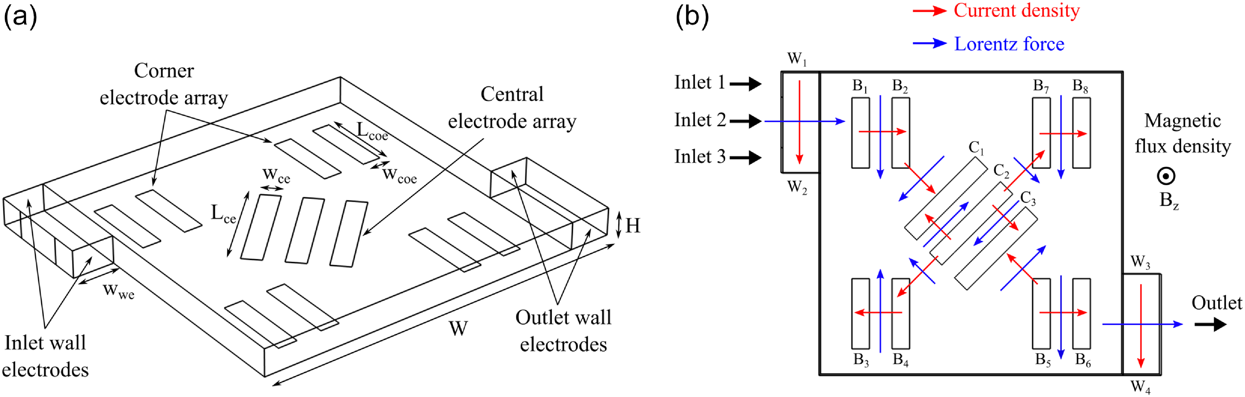
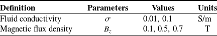
The proposed mixing device has a square profile with dimensions W × W × H, where W = 600 μm and H = 50 μm, as shown in figure 1. We have used two types of electrodes/electrode arrays: (i) base electrode arrays located at the corners (B1 – B8) and in the central region (C1 – C3) and (ii) inlet/outlet wall electrodes (W1 – W4). The geometrical parameters of the electrodes are : Lce = 200 μm, Wce = 35 μm, Lcoe = 140 μm, Wcoe = 35 μm and Wwe = 75 μm. The non-Newtonian behaviour of the fluid was incorporated by employing the Carreau–Yasuda model and both the cases of shear-thinning and shear-thickening fluids have been studied. We have assumed that the device is connected to reservoirs at the inlets and outlet and the fluids are drawn in and expelled out by Lorentz forces, generated by the wall electrodes (W1 – W2 for inlet and W3 – W4 for outlet). After the fluids from different reservoirs have been drawn in, they are forced to traverse a desired route in the compact space of the mixing chamber, such that species mixing is enhanced. The direction of flow is manipulated by controlling the voltages at the base electrode arrays. In the end, the mixture quality is quantified in terms of mixing index η and is tracked at the device outlet over the duration of operation.
Schematic of the proposed MHD micromixer showing the (a) geometric parameters and (b) working principle.
3. Theory
In this section, the necessary equations governing the charge conservation, mass conservation, momentum conservation and species transport are elaborated on in detail.
3.1. Charge conservation
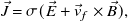
The charge conservation can be imposed by (Jeon et al. Reference Jeon, Massoudi and Kim2017; Chen & Kim Reference Chen and Kim2018)
 \begin{align} \nabla \cdot \vec {J} = 0, \end{align}
where $\vec{J}$
is the current density.
$\vec{J}$
is the current density.
According to Ohm’s law for conducting fluids, the current density ( $\vec{J}$
) can be given by (La et al. Reference La, Kim, Yang, Kim and Kim.2014)
$\vec{J}$
) can be given by (La et al. Reference La, Kim, Yang, Kim and Kim.2014)
 \begin{align} \vec {J} = \sigma (\vec {E} + \vec {v}_f \times \vec {B}), \end{align}
where σ is the fluid conductivity, $\vec{v}$
f
is the fluid velocity and
$\vec{v}$
f
is the fluid velocity and $\vec{B}$
is the magnetic flux density.
$\vec{B}$
is the magnetic flux density.
In Eq. 2, the electric field vector $\vec{E}$
can be expressed as the gradient of a scalar as,
$\vec{E}$
can be expressed as the gradient of a scalar as, $\vec{E}$
= − ∇
$\vec{E}$
= − ∇ $\phi$
, where
$\phi$
, where $\phi$
is the scalar electric potential field. For weak electrolytes, the induced currents in the fluid passing through a magnetic field can be neglected (La et al. Reference La, Kim, Yang, Kim and Kim.2014; Yuan & Isaac Reference Yuan and Isaac2017) and hence the term
$\phi$
is the scalar electric potential field. For weak electrolytes, the induced currents in the fluid passing through a magnetic field can be neglected (La et al. Reference La, Kim, Yang, Kim and Kim.2014; Yuan & Isaac Reference Yuan and Isaac2017) and hence the term $\vec{v}$
f
×
$\vec{v}$
f
× $\vec{B}$
can be neglected. Therefore, the current density for the present study takes the final form
$\vec{B}$
can be neglected. Therefore, the current density for the present study takes the final form
 \begin{align} \vec {J} = -\sigma \nabla \phi . \end{align}
Substituting Eq. 3 in Eq. 1, we obtain the Laplace’s equation for electric potential field given by (Yuan & Isaac Reference Yuan and Isaac2017)
 \begin{align} \nabla ^2 \phi = 0. \end{align}
3.2. Mass conservation
The mass conservation is enforced by the continuity equation, which for a steady and incompressible flow takes the following form (Chen & Kim Reference Chen and Kim2018; La et al. Reference La, Kim, Yang, Kim and Kim.2014):
 \begin{align} \nabla \cdot \vec {v} = 0. \end{align}
3.3. Momentum conservation
The Navier-Stokes equation for the conservation of momentum for an incompressible fluid under steady flow conditions is given by (Chen & Kim Reference Chen and Kim2018). Here $\rho$
is the fluid density,
$\rho$
is the fluid density, $p$
is the pressure,
$p$
is the pressure, $\tau$
is the viscous stress tensor, and
$\tau$
is the viscous stress tensor, and $F_L$
is the Lorentz force vector
$F_L$
is the Lorentz force vector
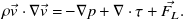 \begin{align} \rho \vec {v}\cdot \nabla \vec {v} = -\nabla p +\nabla \cdot \tau + \vec {F_L}. \end{align}
The non-Newtonian behaviour of the fluid is incorporated by employing the Carreau–Yasuda constitutive relations for fluid viscosity. The Carreau–Yasuda model offers a few advantages over commonly used non-Newtonian models like the power law model. Adding on the features of power law fluids, the Carreau–Yasuda model also helps us to incorporate the zero shear rate viscosity and infinite shear rate viscosity for flows at very low shear rates and at very high shear rates, respectively. The standard form of the viscous stress tensor and the Carreau–Yasuda constitutive relations are given by (Mahapatra et al. Reference Mahapatra, Jana and Bandopadhyay2024)
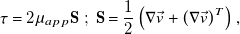 \begin{align} \tau = 2\mu _{app}\mathbf {S} \ ; \ \mathbf {S} = \frac {1}{2}\left ( \nabla \vec {v} + \left ( \nabla \vec {v} \right )^T \right ), \end{align}
 \begin{align} \mu _{app} = \mu _{\infty } + (\mu _0 - \mu _{\infty })[1 + \left (\lambda \dot {\gamma }\right )^a]^{\frac {n-1}{a}}, \end{align}
where μ
app
is the apparent viscosity of the Carreau–Yasuda fluid, $\dot{\gamma}$
is the shear rate and it is defined as the inner product of strain-rate tensor
$\dot{\gamma}$
is the shear rate and it is defined as the inner product of strain-rate tensor $\mathbf {S}$
, i.e.
$\mathbf {S}$
, i.e. $\dot {\gamma } = \sqrt {2\mathbf {S:S}}$
. Here, μ
0 is the zero shear rate viscosity and μ
∞ is the infinite shear rate viscosity and they define the asymptotic limits of the viscosity at very low and very high shear rates (Boyd et al. Reference Boyd, Buick and Green2007). Also,
$\dot {\gamma } = \sqrt {2\mathbf {S:S}}$
. Here, μ
0 is the zero shear rate viscosity and μ
∞ is the infinite shear rate viscosity and they define the asymptotic limits of the viscosity at very low and very high shear rates (Boyd et al. Reference Boyd, Buick and Green2007). Also, $\lambda$
, a and n are the relaxation time, transition parameter and power index, respectively, and together they control the fluid behaviour in the non-Newtonian regime (Boyd et al. Reference Boyd, Buick and Green2007).
$\lambda$
, a and n are the relaxation time, transition parameter and power index, respectively, and together they control the fluid behaviour in the non-Newtonian regime (Boyd et al. Reference Boyd, Buick and Green2007).
The last term ( $\vec {F_L}$
) on the right-hand side of Eq. 6 is the Lorentz force vector and is given by (La et al. Reference La, Kim, Yang, Kim and Kim.2014; Jeon et al. Reference Jeon, Massoudi and Kim2017; Chen et al. Reference Chen, Fan and Kim2019; Yuan & Isaac Reference Yuan and Isaac2017)
$\vec {F_L}$
) on the right-hand side of Eq. 6 is the Lorentz force vector and is given by (La et al. Reference La, Kim, Yang, Kim and Kim.2014; Jeon et al. Reference Jeon, Massoudi and Kim2017; Chen et al. Reference Chen, Fan and Kim2019; Yuan & Isaac Reference Yuan and Isaac2017)
 \begin{align} \vec {F_L}=\vec {J} \times \vec {B}, \end{align}
where $\vec{B}={B_z}\hat {k}$
is the magnetic flux density whose value has been presented in table 2. Using Eq. 3 in Eq. 9, the Lorentz force vector takes the final form (La et al. Reference La, Kim, Yang, Kim and Kim.2014; Yuan & Isaac Reference Yuan and Isaac2017)
$\vec{B}={B_z}\hat {k}$
is the magnetic flux density whose value has been presented in table 2. Using Eq. 3 in Eq. 9, the Lorentz force vector takes the final form (La et al. Reference La, Kim, Yang, Kim and Kim.2014; Yuan & Isaac Reference Yuan and Isaac2017)
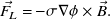 \begin{align} \vec {F_L}=-\sigma \nabla \phi \times \vec {B}. \end{align}
3.4. Transport of species
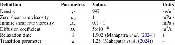
The advection-diffusion equation, given by Eq. 11 (Barman & Bandopadhyay Reference Barman and Bandopadhyay2023; Mahapatra et al. Reference Mahapatra, Jana and Bandopadhyay2024) is solved to find the concentration (c) field of a passive, neutrally buoyant species with a diffusion coefficient of D c , whose magnitude is given in table 1.
Properties of the Carreau–Yasuda fluid used for simulations
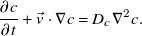 \begin{align} \frac {\partial c}{\partial t} + \vec {v} \cdot \nabla c = {D_c}\nabla ^2 {c}. \end{align}
Operating conditions for MHD flow used for simulations
The quality of mixing is quantified by calculating the mixing index (η) at the device outlet given by (Faradonbeh et al. Reference Faradonbeh, Rabiei, Rabiei, Goodarzi, Safaei and Lin2022)
 \begin{align} \eta = \left [1-\sqrt {\frac {\int _{A} \left (c-c^*\right )^2\, dA}{\int _{A} (c^*)^2 \, dA} }\right ], \end{align}
where ${c^*}$
represents the homogeneously mixed state and is fixed at 0.5 for the present study. Here, A represents the total area of the outlet port of the device.
${c^*}$
represents the homogeneously mixed state and is fixed at 0.5 for the present study. Here, A represents the total area of the outlet port of the device.
3.5. Boundary conditions
A voltage of $\phi$
e
is applied on the electrodes and its magnitude depends on the type of electrode. All the remaining walls and boundaries of the device are assumed to be electrically insulated
$\phi$
e
is applied on the electrodes and its magnitude depends on the type of electrode. All the remaining walls and boundaries of the device are assumed to be electrically insulated
 \begin{align} \phi = \phi _e \ ; \ (\hat {n}\cdot \nabla \phi )_{walls} = 0. \end{align}
Since the flow is not pressure driven, the inlet and outlets of the device are at kept at zero pressure (zero pressure difference with the ambient) and all the walls and boundaries of the device are set with a no-slip boundary condition
 \begin{align} p_{\mathrm {inlet}} = p_{\mathrm {outlet}} = 0 \ ; \ \vec {v}_{walls} = 0. \end{align}
For the mixing problem, we have considered three different inlet ports, as shown in figure 1b. We have made the assumption that the inlet port 2 draws in a conducting fluid from a reservoir rich in a test species, while inlet ports 1 and 3 draw in the same fluid but devoid of any species. An outflow condition is set at the outlet and all the remaining walls are set with a no-flux boundary condition
 \begin{align} c_{\mathrm {I1}} = c_{\mathrm {I3}} = 0 \ ; \ c_{\mathrm {I2}} = 1 \ ; \ (\hat {n} \cdot \nabla c)_{walls} = 0, \end{align}
where the subscripts I1, I2 and I3 refer to the three inlet ports.
4. Numerical modelling
The finite element framework of COMSOL Multiphysics 6.2 has been used for the numerical analysis. The electric currents interface was used to solve for the electric potential field, the laminar flow interface was used for solving the flow field and the concentration field was solved using the transport of diluted species interface. The order of the shape functions for the electric potential, flow of fluids and concentration fields were quadratic, P2 (second order element for velocity) + P1 (first order element for pressure) and linear, respectively. The electric potential and flow field were solve in a coupled manner using a stationary solver, while a time-dependent solver was used for the transport of species. Initially, a mesh independence test was performed in order to find a suitable meshing sequence such that a balance is struck between solution accuracy and computational effort. Thereafter, the numerical model was validated against a published work in the literature involving the same physics.
4.1. Meshing
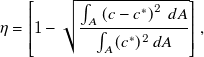
For meshing of the computational domain, extremely fine mesh was chosen for the electrodes and slightly coarser mesh was chosen for the domain and remaining walls. Figure 2 presents a representative mesh of the computational domain. Thereafter, a mesh independence test was performed to obtain a sufficiently fine mesh, such that a balance is struck between computational effort and solution accuracy. The results of the test are presented in table 3 and they indicate that the solutions do not show much deviation on increasing the number of mesh elements beyond 8.32 × 10⁵. Therefore, a total of 8.32 × 10⁵ mesh elements have been used for all the simulations.
Mesh independence test results
Representative meshes of the computational domain with a fine mesh on the electrodes and slightly coarser mesh on the walls : (a) top view (b) bottom view.
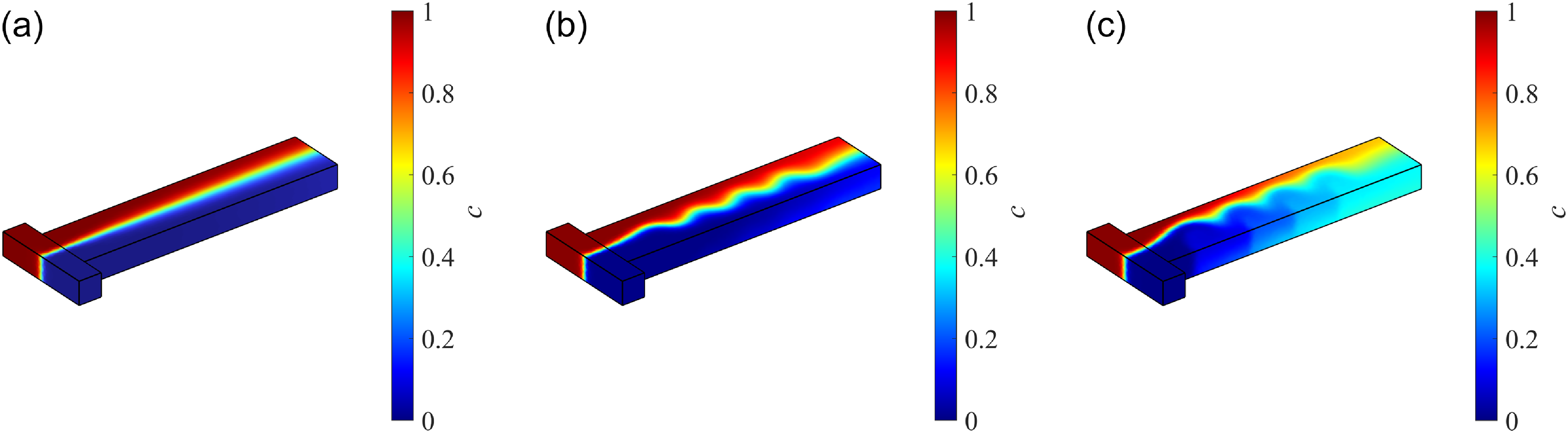
Concentration field given by the present numerical model for a case of Newtonian fluid in an MHD T-channel for (a) axial flow, (b) sinusoidal flow and (c) multi-vortical flow. The results are in excellent agreement with those obtained by La et al. (Reference La, Kim, Yang, Kim and Kim.2014) (see figure 11 of the article by La et al. (Reference La, Kim, Yang, Kim and Kim.2014)).
4.2. Model validation
The numerical model was validated with the results obtained by La et al. (Reference La, Kim, Yang, Kim and Kim.2014) in terms of the concentration field in a T-channel, working on the principles of MHD and the standard deviation of species concentration at the outlet. Concentration fields for three different flow types – axial, sinusoidal and multi-vortical were evaluated and the results given by the present model are presented in figure 3, which are in excellent agreement with that obtained by La et al. (Reference La, Kim, Yang, Kim and Kim.2014) (see figure 11 of their article).
Model validation : standard deviations of concentration fields at microchannel outlet
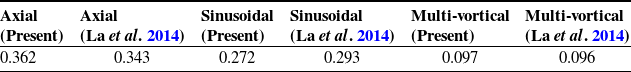
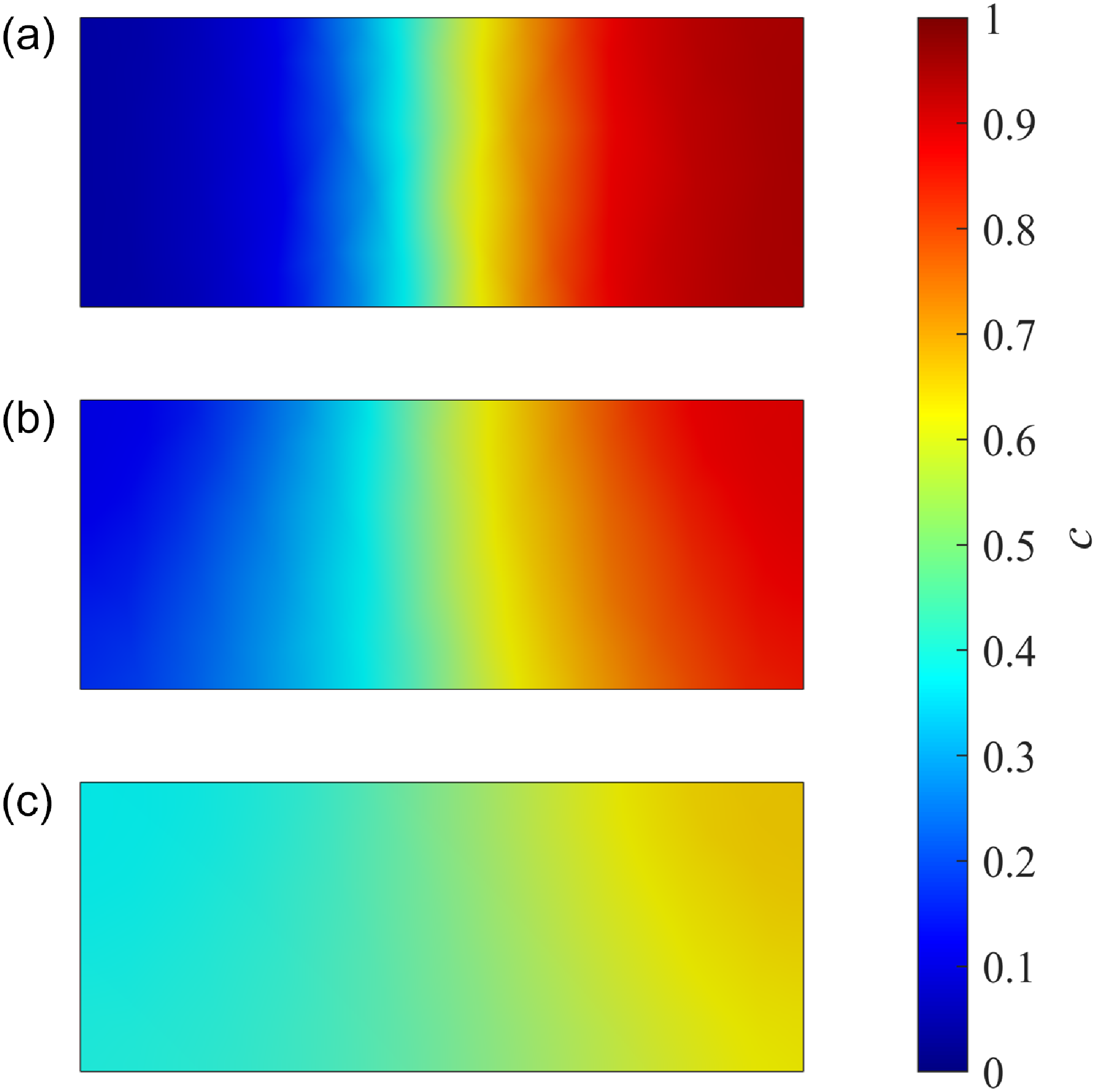
Figure 4 presents the concentration fields at the channel outlet for axial, sinusoidal and multi-vortical flows and these are in very good agreement with the results obtained by La et al. (Reference La, Kim, Yang, Kim and Kim.2014) (see figure 12 of their article). The standard deviations of species concentration at the outlet were calculated and compared with that obtained by La et al. (Reference La, Kim, Yang, Kim and Kim.2014), the results are presented in table 4. Based on the good agreement shown by the results presented in figure 3, figure 4 and table 4, we conclude our numerical model as validated.
Concentration field at the microchannel outlet given by the present numerical model for a case of a Newtonian fluid in an MHD T-channel for (a) axial flow, (b) sinusoidal flow and (c) multi-vortical flow. The results are in excellent agreement with those obtained by La et al. (Reference La, Kim, Yang, Kim and Kim.2014) (see figure 12 of the article by La et al. (Reference La, Kim, Yang, Kim and Kim.2014)).
5. Results and discussions
In order to gain a better understanding of the underlying physics of MHD mixing in Carreau–Yasuda fluids, different numerical investigations, each focussing on a different aspect of MHD mixing, were conducted and the results are presented along with respective discussions in the following sections.
5.1. Effect of flow pattern on species mixing
First, we demonstrate how a complex flow pattern, generated by an optimum combination of voltages applied to the electrodes, has the potential to induce rapid and homogeneous mixing. For this, the electrode potentials ( $\phi$
e
) were set at :
$\phi$
e
) were set at : $\phi$
w1 =
$\phi$
w1 = $\phi$
w3 = 0 V,
$\phi$
w3 = 0 V, $\phi$
w2 =
$\phi$
w2 = $\phi$
w4 = 10 V,
$\phi$
w4 = 10 V, $\phi$
b1 =
$\phi$
b1 = $\phi$
b4 =
$\phi$
b4 = $\phi$
b5 =
$\phi$
b5 = $\phi$
b7 = 7.5 V,
$\phi$
b7 = 7.5 V, $\phi$
b2 =
$\phi$
b2 = $\phi$
b3 =
$\phi$
b3 = $\phi$
b6 =
$\phi$
b6 = $\phi$
b8 = 0 V,
$\phi$
b8 = 0 V, $\phi$
c2 =
$\phi$
c2 = $\phi$
c3 = 10 V and
$\phi$
c3 = 10 V and $\phi$
c1 = 0 V.
$\phi$
c1 = 0 V.
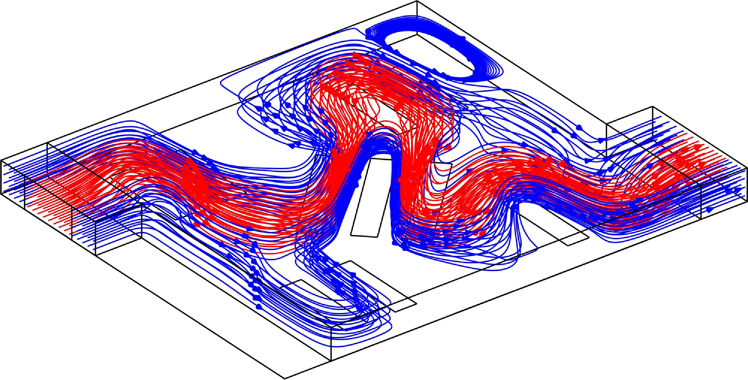
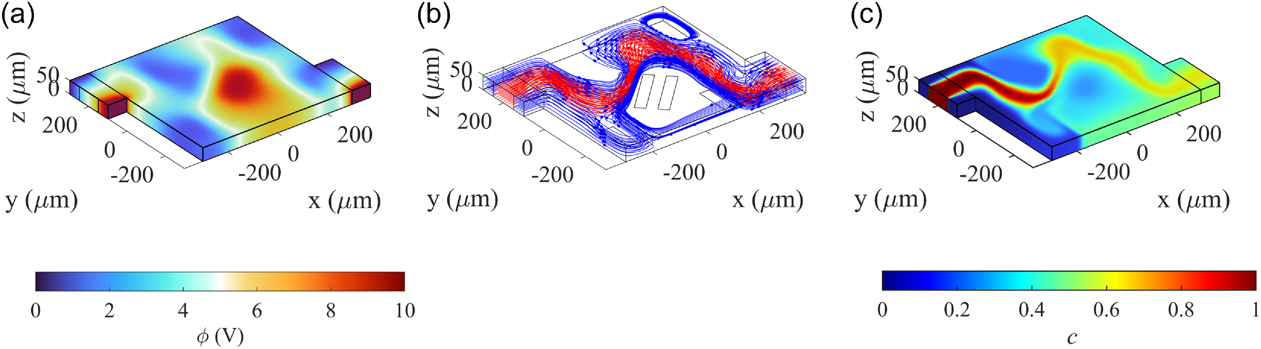
Results showcasing the effect of flow pattern on mixing: (a) electric potential ( $\phi$
) field, (b) streamlines from inlet 1 and 3 (in blue indicating no species) and inlet 2 (in red indicating rich in species) and (c) concentration field (c) (after t = 10 s). The fluid conductivity (σ) and magnetic flux density (Bz) were set at 0.1 S/m and 0.7 T respectively. The infinite shear rate viscosity (μ∞) was set at 0 mPa·s and the zero shear rate viscosity (μ0) was taken as 1 mPa·s while the power index (n) was set at 0.8.
$\phi$
) field, (b) streamlines from inlet 1 and 3 (in blue indicating no species) and inlet 2 (in red indicating rich in species) and (c) concentration field (c) (after t = 10 s). The fluid conductivity (σ) and magnetic flux density (Bz) were set at 0.1 S/m and 0.7 T respectively. The infinite shear rate viscosity (μ∞) was set at 0 mPa·s and the zero shear rate viscosity (μ0) was taken as 1 mPa·s while the power index (n) was set at 0.8.
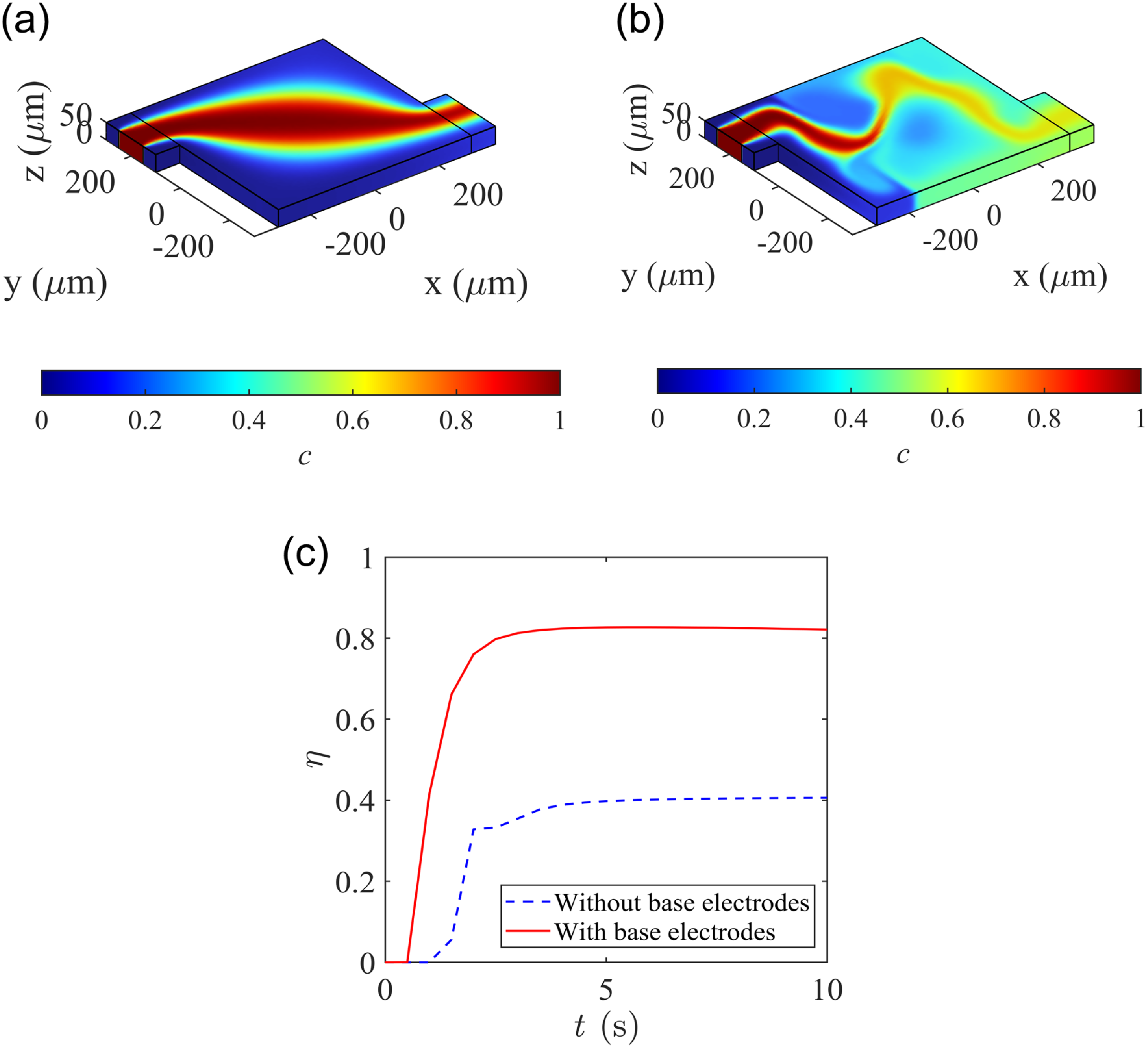
Concentration field after t = 10 s for cases : (a) without base electrodes, (b) with base electrodes and (c) comparison of evolution of η over a duration of 10 s for cases (a) and (b).
The chosen voltage combination at the electrodes results in an electric potential ( $\phi$
) field as shown in figure 5a. The generated flow pattern takes the form shown in figure 5b due to the effect of the Lorentz forces on the conducting Carreau–Yasuda fluid (power index was set at n = 0.8). The fluid streams incoming from the inlets (red denotes the fluid rich in test species and blue denotes fluid with no species) are forced to traverse a longer path in a compact space, which not only results in enhanced advective transport of the species to different sections of the chamber but also results in increased interfacial area. Larger interfacial area causes greater molecular diffusion, ultimately leading to better mixing. Figure 5c presents the species concentration field (c) in the chamber after 10 s from the introduction of species, and we note that a very good quality mixture is obtained at the outlet (η = 0.82).
$\phi$
) field as shown in figure 5a. The generated flow pattern takes the form shown in figure 5b due to the effect of the Lorentz forces on the conducting Carreau–Yasuda fluid (power index was set at n = 0.8). The fluid streams incoming from the inlets (red denotes the fluid rich in test species and blue denotes fluid with no species) are forced to traverse a longer path in a compact space, which not only results in enhanced advective transport of the species to different sections of the chamber but also results in increased interfacial area. Larger interfacial area causes greater molecular diffusion, ultimately leading to better mixing. Figure 5c presents the species concentration field (c) in the chamber after 10 s from the introduction of species, and we note that a very good quality mixture is obtained at the outlet (η = 0.82).
On comparing the results for the present case of species mixing (as shown in figure 5c) with that of a case with no base electrodes it is conclusive that the proposed MHD system performs far superior in terms of species distribution in the chamber. Figure 6 presents the concentration fields for cases with no base electrodes (figure 6a) and with base electrodes (figure 6b). Wall electrodes (W1 – W4) were used in both cases for the purpose of drawing in and expelling out the fluid streams. As shown in figure 6c, the mixture quality at the outlet is far superior (η = 0.82 after t = 10 s) compared with the case with no base electrodes (η = 0.41 after t = 10 s). Once again, this is because of the complex flow path traversed by the incoming fluids in the latter case, which increases the interfacial area to a great degree. The greater the interfacial area, the higher is the rate of molecular diffusion and the faster is the transport of species across the concentration gradients.
5.2. Effect of power index on flow parameters
In the previous section, we have seen the efficacy of MHD mixing for a case of shear-thinning Carreau–Yasuda fluid. We know that, for a Carreau–Yasuda fluid, the power index plays a crucial role in determining the flow behaviour according to equations 6, 7 and 8. In this section, we discuss the simulation results, highlighting the effect of the power index (n) of the Carreau–Yasuda fluid on the different flow parameters. Figure 7 presents the effect of the power index on different flow parameters like the velocity magnitude (U), shear rate ( $\dot{\gamma}$
) and apparent viscosity (μ
app
) along a cutline close to the bottom wall, at a height of H/10 with x = 0 and y ranging from −W/2 to W/2. The voltages at different electrodes were set at:
$\dot{\gamma}$
) and apparent viscosity (μ
app
) along a cutline close to the bottom wall, at a height of H/10 with x = 0 and y ranging from −W/2 to W/2. The voltages at different electrodes were set at: $\phi$
w1 =
$\phi$
w1 = $\phi$
w3 = 0 V,
$\phi$
w3 = 0 V, $\phi$
w2 =
$\phi$
w2 = $\phi$
w4 = 10 V,
$\phi$
w4 = 10 V, $\phi$
b1 =
$\phi$
b1 = $\phi$
b4 =
$\phi$
b4 = $\phi$
b5 =
$\phi$
b5 = $\phi$
b7 = 7.5 V,
$\phi$
b7 = 7.5 V, $\phi$
b2 =
$\phi$
b2 = $\phi$
b3 =
$\phi$
b3 = $\phi$
b6 =
$\phi$
b6 = $\phi$
b8 = 0 V,
$\phi$
b8 = 0 V, $\phi$
c2 =
$\phi$
c2 = $\phi$
c3 = 10 V and
$\phi$
c3 = 10 V and $\phi$
c1 = 0 V.
$\phi$
c1 = 0 V.
Effect of power index on different flow parameters : (a) velocity magnitude (U) vs y, (b) shear rate ( $\dot{\gamma}$
) vs y, (c) apparent viscosity (μapp) vs y along a cutline in the domain. The fluid conductivity (σ) and magnetic flux density (Bz) were set at 0.01 S/m and 0.1 T, respectively. The infinite shear rate viscosity (μ∞) was taken as 0 mPa·s, the zero shear rate viscosity (μ0) was set at 1 mPa·s, the relaxation time (
$\dot{\gamma}$
) vs y, (c) apparent viscosity (μapp) vs y along a cutline in the domain. The fluid conductivity (σ) and magnetic flux density (Bz) were set at 0.01 S/m and 0.1 T, respectively. The infinite shear rate viscosity (μ∞) was taken as 0 mPa·s, the zero shear rate viscosity (μ0) was set at 1 mPa·s, the relaxation time ( $\lambda$
) was set at 1.902 s and the transition parameter (a) was chosen as 1.25.
$\lambda$
) was set at 1.902 s and the transition parameter (a) was chosen as 1.25.
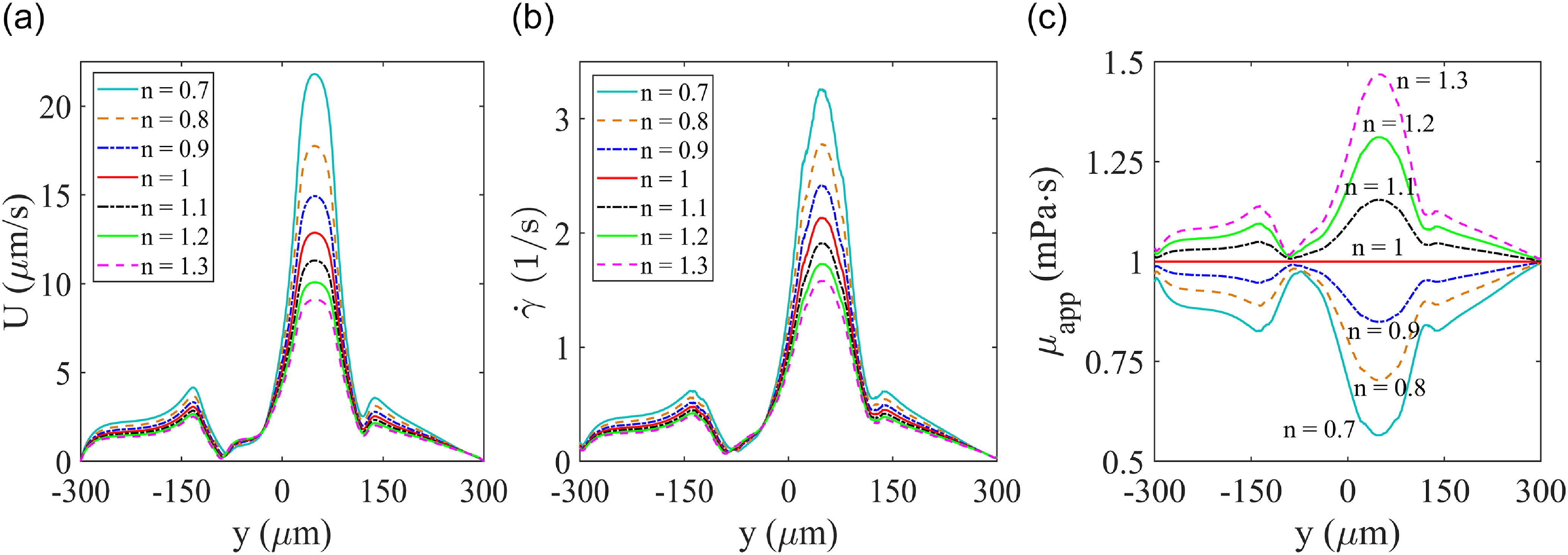
Under the same set of operating parameters, the velocity magnitude along the cutline (see figure 7a) is highest for a shear-thinning fluid (n = 0.7) and the lowest for a shear-thickening fluid (n = 1.3). The same trend is observed for the variation of shear rate ( $\dot{\gamma}$
) along the cutline (see figure 7b). These characteristic trends shown by U and
$\dot{\gamma}$
) along the cutline (see figure 7b). These characteristic trends shown by U and $\dot{\gamma}$
are due to the changes in the apparent viscosity μ
app
, which again depends on
$\dot{\gamma}$
are due to the changes in the apparent viscosity μ
app
, which again depends on $\dot{\gamma}$
. The apparent viscosity increases with increase in shear rates
$\dot{\gamma}$
. The apparent viscosity increases with increase in shear rates $\dot{\gamma}$
for shear-thickening fluids and decreases with increase in
$\dot{\gamma}$
for shear-thickening fluids and decreases with increase in $\dot{\gamma}$
for shear-thinning fluids. The drop in μ
app
along the cutline causes U and
$\dot{\gamma}$
for shear-thinning fluids. The drop in μ
app
along the cutline causes U and $\dot{\gamma}$
to undergo significant increment and vice versa. The results presented in figure 7 give valuable insights into the effect of rheology on different flow parameters and will be very useful for study of MHD flow manipulation of different types of non-Newtonian fluids in real world experimental scenarios.
$\dot{\gamma}$
to undergo significant increment and vice versa. The results presented in figure 7 give valuable insights into the effect of rheology on different flow parameters and will be very useful for study of MHD flow manipulation of different types of non-Newtonian fluids in real world experimental scenarios.
5.3. Non-dimensional analysis
According to Eq. 10, the different factors influencing the magnitude of the Lorentz forces are the fluid conductivity (σ), magnetic flux density ( $\vec{B}$
) and the gradient of the
$\vec{B}$
) and the gradient of the $\phi$
field. The choice of voltages at the electrodes affects the spatial distribution of
$\phi$
field. The choice of voltages at the electrodes affects the spatial distribution of $\phi$
(∇
$\phi$
(∇ $\phi$
), which in turn affects the magnitude of the Lorentz force. In order to capture the overall impact of varying operating parameters on mixing, we take the help of non-dimensional numbers. The results presented in this section will be very useful in the design and fabrication of MHD devices based on the present work for different sets of operating conditions.
$\phi$
), which in turn affects the magnitude of the Lorentz force. In order to capture the overall impact of varying operating parameters on mixing, we take the help of non-dimensional numbers. The results presented in this section will be very useful in the design and fabrication of MHD devices based on the present work for different sets of operating conditions.
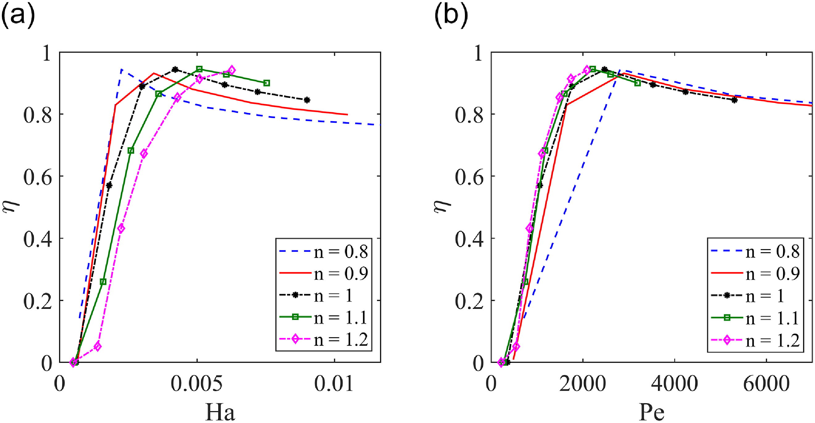
Effect of (a) Hartmann (Ha) number and (b) Péclet (Pe) number on the mixing index (η) at different values of the power index (n). The infinite shear rate viscosity (μ∞) was taken as 0 mPa·s, the zero shear rate viscosity (μ0) was set at 1 mPa·s, the relaxation time ( $\lambda$
) was set at 1.902 s and the transition parameter (a) was chosen as 1.25.
$\lambda$
) was set at 1.902 s and the transition parameter (a) was chosen as 1.25.
First, let us discuss about two popular non-dimensional numbers in MHD mixing, namely, the Hartmann number and the Péclet number. The Hartmann number is ratio of Lorentz forces to viscous forces and is given by Ha = (σB
z
2 L $_{c}^2/\mu _{c})^{\frac {1}{2}}$
, while the Péclet number, given by Pe = Uc Lc/D
c
, is the ratio of advective mass transport to diffusive mass transport. Unlike electroosmotic flow, since there is no natural velocity scale for the present case of MHD, the characteristic velocity, U
c
, is taken equal to U
max
, which is the maximum velocity in the domain for a given set of operating conditions. Here, W is chosen as the characteristic length L
c
and the characteristic viscosity is evaluated as
$_{c}^2/\mu _{c})^{\frac {1}{2}}$
, while the Péclet number, given by Pe = Uc Lc/D
c
, is the ratio of advective mass transport to diffusive mass transport. Unlike electroosmotic flow, since there is no natural velocity scale for the present case of MHD, the characteristic velocity, U
c
, is taken equal to U
max
, which is the maximum velocity in the domain for a given set of operating conditions. Here, W is chosen as the characteristic length L
c
and the characteristic viscosity is evaluated as $\mu _c = \overline \mu _{app} = (\mu _{app,min} + \mu _{app,max})/2$
. Figure 8a presents the effect of Hartmann (Ha) number on mixing index (η), where η has been evaluated at the device outlet. For the case of Newtonian fluids (n = 1), the mixing index increases with the increase in Hartmann number up to a certain critical limit and slightly decreases thereafter. As the power index (n) increases above 1 (shear-thickening nature), the critical limit undergoes a shift towards slightly higher Ha. The opposite effect is observed as n decreases below 1 (shear-thinning nature), when the critical limit shifts towards low Ha. As shown in figure 8b, a similar trend is demonstrated by η in response to the variation in Pe. The slight drop in the mixture quality at high Ha and Pe is primarily due to rapid transport of the unmixed streams to the outlet. Therefore, in any type of Carreau–Yasuda fluid (shear thinning, Newtonian or shear thickening), the operating parameters should be chosen such that Ha and Pe are in the vicinity of their critical values for that particular power index and this condition ensures the best mixing performance for the proposed MHD mixing device.
$\mu _c = \overline \mu _{app} = (\mu _{app,min} + \mu _{app,max})/2$
. Figure 8a presents the effect of Hartmann (Ha) number on mixing index (η), where η has been evaluated at the device outlet. For the case of Newtonian fluids (n = 1), the mixing index increases with the increase in Hartmann number up to a certain critical limit and slightly decreases thereafter. As the power index (n) increases above 1 (shear-thickening nature), the critical limit undergoes a shift towards slightly higher Ha. The opposite effect is observed as n decreases below 1 (shear-thinning nature), when the critical limit shifts towards low Ha. As shown in figure 8b, a similar trend is demonstrated by η in response to the variation in Pe. The slight drop in the mixture quality at high Ha and Pe is primarily due to rapid transport of the unmixed streams to the outlet. Therefore, in any type of Carreau–Yasuda fluid (shear thinning, Newtonian or shear thickening), the operating parameters should be chosen such that Ha and Pe are in the vicinity of their critical values for that particular power index and this condition ensures the best mixing performance for the proposed MHD mixing device.
Simulation results depicting the (a) evolution of mixing index (η) at the device outlet at different viscosity ratios (β) and (b) variation of characteristic velocity (Uc) with viscosity ratio (β). The magnetic flux density (Bz) was taken as 0.7 T, the fluid conductivity (σ) was set at 0.1 S/m and the power index (n) was fixed at 0.8.
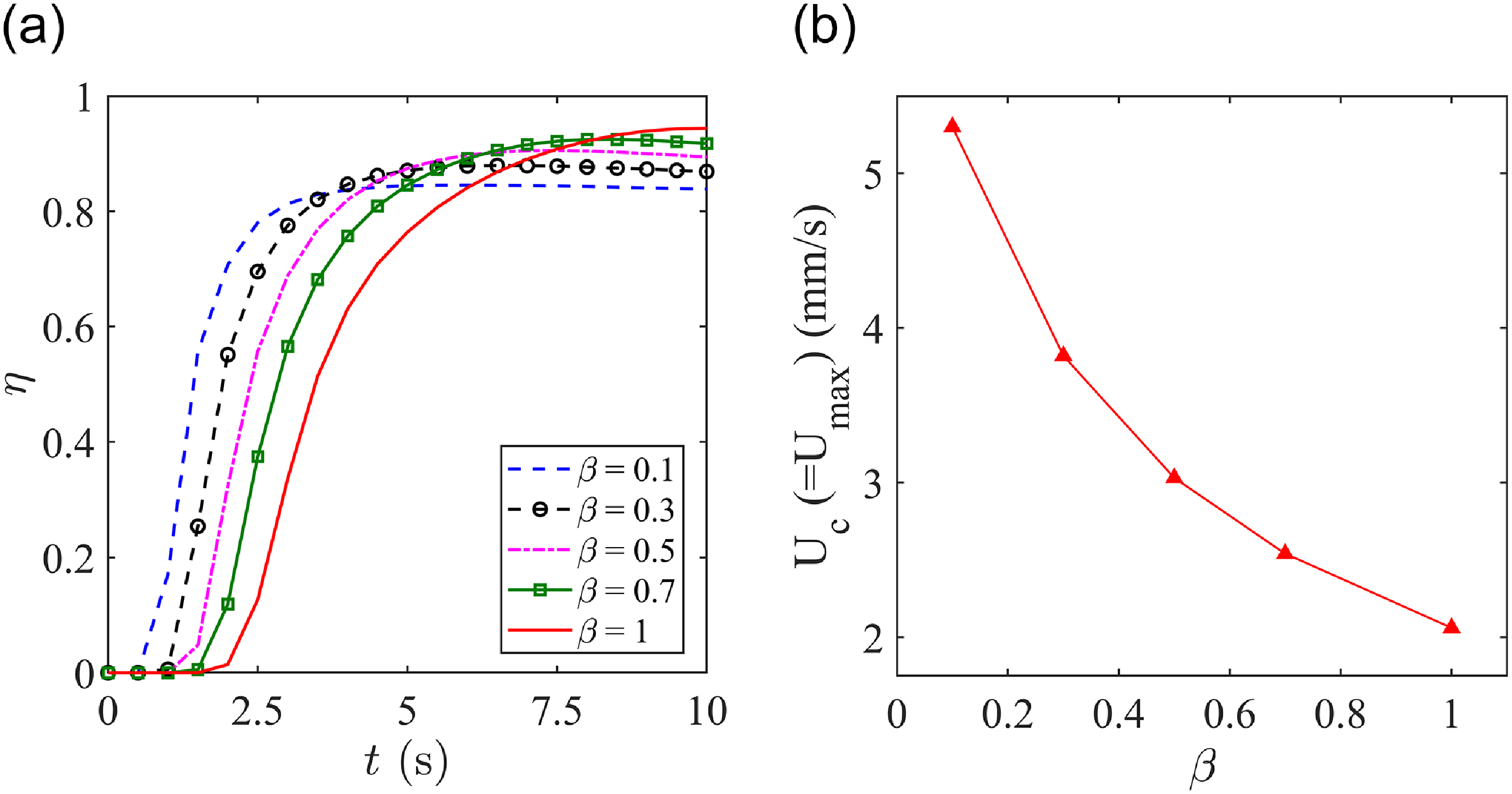
Another important non-dimensional number to be considered is the viscosity ratio (β), which is defined as the ratio of infinite shear rate viscosity to the zero shear rate viscosity, i.e. β = μ ∞/μ 0. For simulations, the zero shear rate viscosity was fixed at 1 mPa·s while μ ∞ was varied by different factors. Figure 9a presents the effect of varying viscosity ratio (β) on mixing index and we note that the mixture quality gets better as viscosity ratio increases. A lower value of β indicates a lower value of μ ∞ and vice versa. In figure 9a, we also note that the mixing index at the outlet increases with time and reaches a steady value for all the cases. Fluids with lower magnitudes of β, demonstrate better and rapid mixing behaviour in the initial stages while the fluids with higher magnitudes of β demonstrate a slightly better performance in the later stages. At high values of β, the overall viscosity of the Carreau–Yasuda fluid increases, resulting in a drop of the characteristic velocity of the device. Although this results in better diffusion of species, the overall impact on the mixture quality is is not substantial.
5.4. Effect of relaxation time ( $\lambda$
) on mixing performance
$\lambda$
) on mixing performance

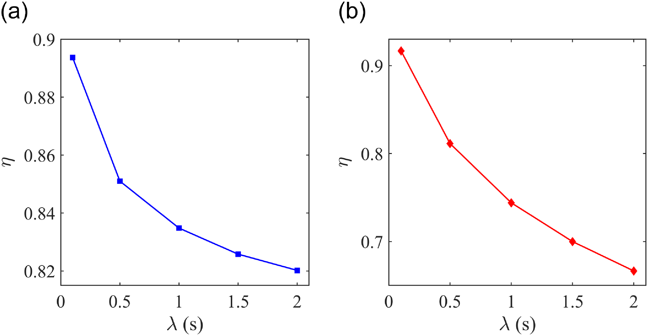
Figure 10 presents the effect of relaxation time ( $\lambda$
) on the mixing index (η) for a case of (a) shear-thinning (n = 0.8) and (b) shear-thickening fluids (n = 1.2). As seen in figure 10, the mixture quality drops with the increase in relaxation time for both shear-thinning (see figure 10a) and shear-thickening (see figure 10b) fluids. The drop in η is more significant for the case of a shear-thickening fluid (≈ 27.3 %) as compared with the case of a shear-thinning fluid (≈ 8.22 %). The higher the value of
$\lambda$
) on the mixing index (η) for a case of (a) shear-thinning (n = 0.8) and (b) shear-thickening fluids (n = 1.2). As seen in figure 10, the mixture quality drops with the increase in relaxation time for both shear-thinning (see figure 10a) and shear-thickening (see figure 10b) fluids. The drop in η is more significant for the case of a shear-thickening fluid (≈ 27.3 %) as compared with the case of a shear-thinning fluid (≈ 8.22 %). The higher the value of $\lambda$
, the greater is the departure from Newtonian behaviour and the greater is the time taken to achieve a state of equilibrium. Hence, for fluids with higher characteristic
$\lambda$
, the greater is the departure from Newtonian behaviour and the greater is the time taken to achieve a state of equilibrium. Hence, for fluids with higher characteristic $\lambda$
, species mixing might be low for a given set of operating conditions, in which case the operating parameters can be optimised to improve the mixture quality.
$\lambda$
, species mixing might be low for a given set of operating conditions, in which case the operating parameters can be optimised to improve the mixture quality.
Variation of mixing index (η) at 10 s with relaxation time ( $\lambda$
) for (a) shear thinning, n = 0.8 and (b) shear thickening, n = 1.2. The infinite shear rate viscosity (μ∞) was taken as 0 mPa·s, the zero shear rate viscosity (μ0) was set at 1 mPa·s and the transition parameter (a) was chosen as 1.25.
$\lambda$
) for (a) shear thinning, n = 0.8 and (b) shear thickening, n = 1.2. The infinite shear rate viscosity (μ∞) was taken as 0 mPa·s, the zero shear rate viscosity (μ0) was set at 1 mPa·s and the transition parameter (a) was chosen as 1.25.
5.5. Effect of electrode configuration on flow pattern and mixing
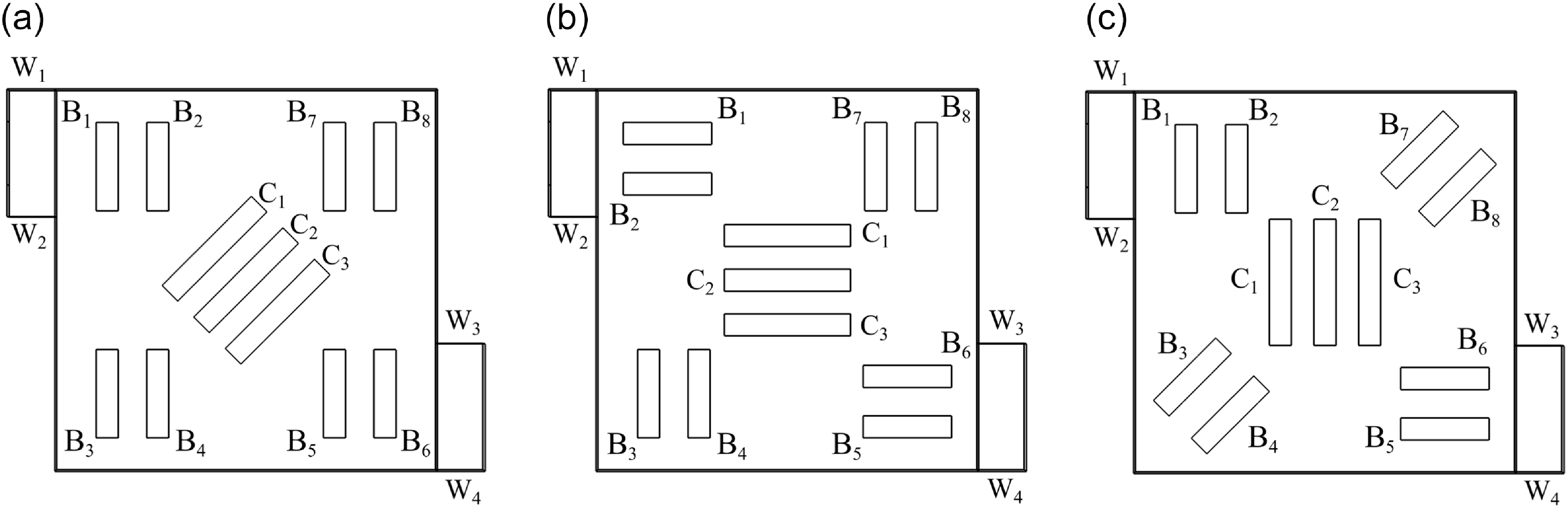
Flow control and manipulation is one the most desired features of MHD based devices and is crucial when it comes to applications in mixing. In this section, we discuss the results of numerical investigations, focused on flow path manipulation and its subsequent effect on species mixing. Figure 11 presents the schematics of three different electrode configurations under consideration.
Schematics of different electrode configurations: (a) configuration-I (C-I), (b) configuration-II (C-II) and (c) configuration-III (C-III).
The electrode voltage combinations for the three configurations are as follows:
(i) Configuration-I (C-I) : $\phi$
w1 =
$\phi$
w1 = $\phi$
w3 = 0 V,
$\phi$
w3 = 0 V, $\phi$
w2 =
$\phi$
w2 = $\phi$
w4 = 10 V,
$\phi$
w4 = 10 V, $\phi$
b1 =
$\phi$
b1 = $\phi$
b4 =
$\phi$
b4 = $\phi$
b5 =
$\phi$
b5 = $\phi$
b7 = 7.5 V,
$\phi$
b7 = 7.5 V, $\phi$
b2 =
$\phi$
b2 = $\phi$
b3 =
$\phi$
b3 = $\phi$
b6 =
$\phi$
b6 = $\phi$
b8 = 0 V,
$\phi$
b8 = 0 V, $\phi$
c1 =
$\phi$
c1 = $\phi$
c3 = 0 V and
$\phi$
c3 = 0 V and $\phi$
c2 = 10 V.
$\phi$
c2 = 10 V.
(ii) Configuration-II (C-II) : $\phi$
w1 =
$\phi$
w1 = $\phi$
w3 = 0 V,
$\phi$
w3 = 0 V, $\phi$
w2 =
$\phi$
w2 = $\phi$
w4 = 10 V,
$\phi$
w4 = 10 V, $\phi$
b1 =
$\phi$
b1 = $\phi$
b4 =
$\phi$
b4 = $\phi$
b6 =
$\phi$
b6 = $\phi$
b8 = 0 V,
$\phi$
b8 = 0 V, $\phi$
b2 =
$\phi$
b2 = $\phi$
b3 =
$\phi$
b3 = $\phi$
b5 =
$\phi$
b5 = $\phi$
b7 = 7.5 V,
$\phi$
b7 = 7.5 V, $\phi$
c1 =
$\phi$
c1 = $\phi$
c3 = 10 V and
$\phi$
c3 = 10 V and $\phi$
c2 = 0 V.
$\phi$
c2 = 0 V.
(iii) Configuration-III (C-III) : $\phi$
w1 =
$\phi$
w1 = $\phi$
w3 = 0 V,
$\phi$
w3 = 0 V, $\phi$
w2 =
$\phi$
w2 = $\phi$
w4 = 10 V,
$\phi$
w4 = 10 V, $\phi$
b1 =
$\phi$
b1 = $\phi$
b3 =
$\phi$
b3 = $\phi$
b6 =
$\phi$
b6 = $\phi$
b8 = 0 V,
$\phi$
b8 = 0 V, $\phi$
b2 =
$\phi$
b2 = $\phi$
b4 =
$\phi$
b4 = $\phi$
b5 =
$\phi$
b5 = $\phi$
b7 = 7.5 V,
$\phi$
b7 = 7.5 V, $\phi$
c1 =
$\phi$
c1 = $\phi$
c3 = 0 V and
$\phi$
c3 = 0 V and $\phi$
c2 = 10 V.
$\phi$
c2 = 10 V.
Flow patterns generated by different electrode configurations: (a) configuration-I (C-I), (b) configuration-II (C-II) and (c) configuration-III (C-III). Concentration fields after t = 10 s for (d) C-I, (e) C-II and (f) C-III. The fluid conductivity σ) and magnetic flux density (Bz) were set at 0.1 S/m and 0.5 T respectively and the power index (n) was set at 1. The infinite shear rate viscosity (μ∞) was taken as 0 mPa·s, the zero shear rate viscosity (μ0) was set at 1 mPa·s, the relaxation time ( $\lambda$
) was set at 1.902 s and the transition parameter (a) was chosen as 1.25.
$\lambda$
) was set at 1.902 s and the transition parameter (a) was chosen as 1.25.
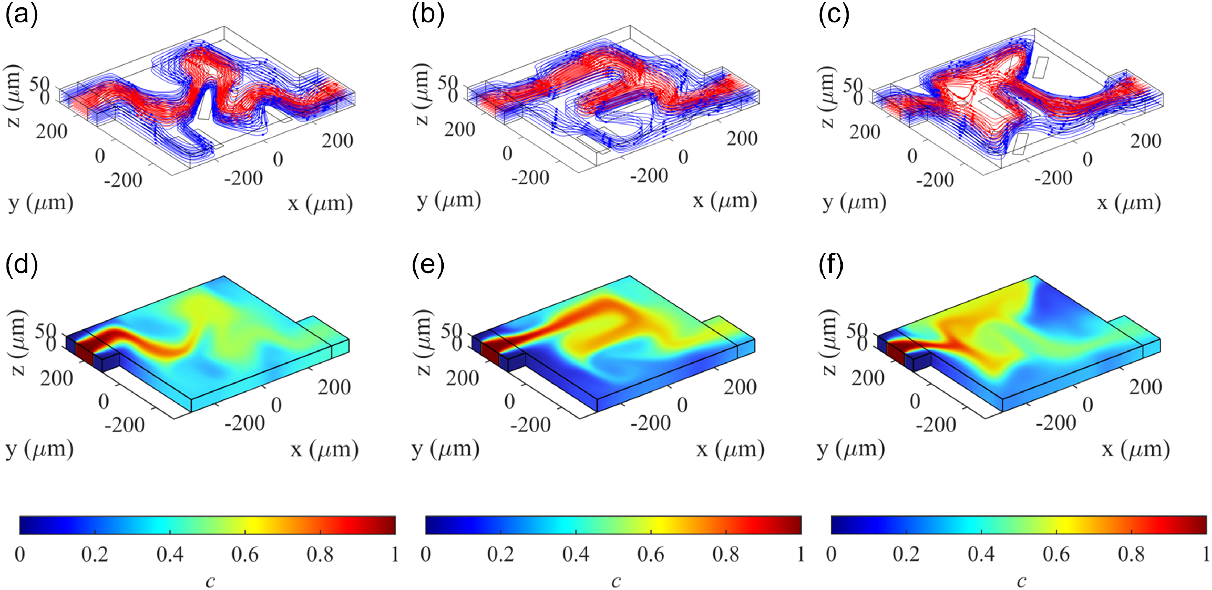
Figure 12a–c presents the streamlines of the fluids drawn in through inlet 1 (blue), inlet 2 (red) and inlet 3 (blue), with species rich fluid being drawn in through inlet 2. As mentioned earlier, the objective is to manipulate the flow to traverse a complex and longer path, in a compact region, such that the species gets readily advected to different sections in the chamber and has sufficient time to diffuse. As seen in figure 12d–f, the species is well distributed throughout the domain for all three configurations compared with a case with no base electrodes to manipulate the flow (see figure 6a). All the results presented in figure 12, were obtained for a case with n = 1, i.e. for a Newtonian fluid, and we note that C-I performs better in terms of homogeneous mixing (η = 0.86) compared with C-II (η = 0.80) and C-III (η = 0.82).
Evolution of η over time for electrode configurations C-I, C-II and C-III for (a) shear-thinning (n = 0.8), (b) Newtonian (n = 1) and (c) shear-thickening (n = 1.2) fluids. The mixing indices (η) were evaluated at the device outlet over a duration of 10 s. The fluid conductivity (σ) and magnetic flux density (Bz) were set at 0.1 S/m and 0.5 T respectively for all the cases. The infinite shear rate viscosity (μ∞) was taken as 0 mPa·s, the zero shear rate viscosity (μ0) was set at 1 mPa·s, the relaxation time ( $\lambda$
) was set at 1.902 s and the transition parameter (a) was chosen as 1.25.
$\lambda$
) was set at 1.902 s and the transition parameter (a) was chosen as 1.25.
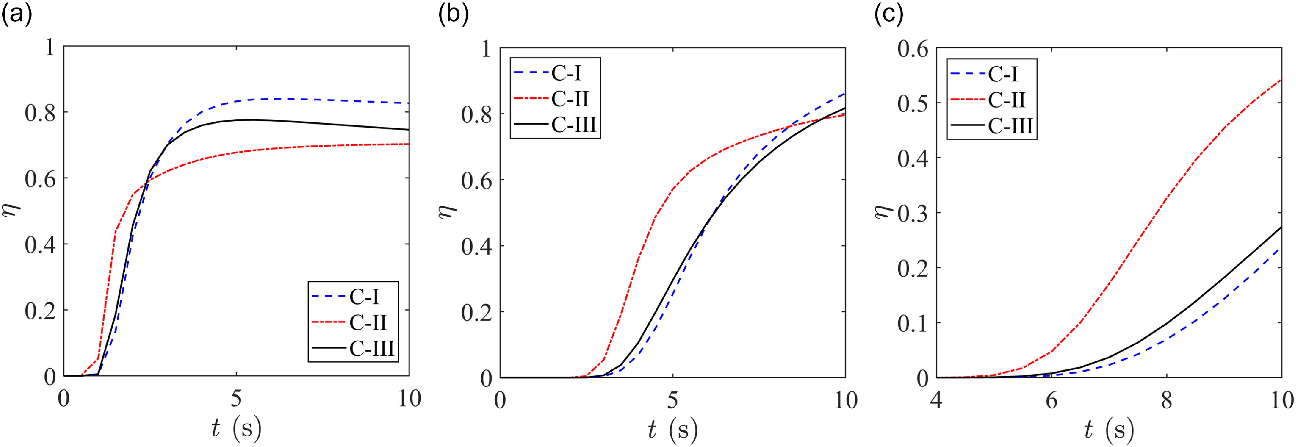
The mixing performances for configurations C-I, C-II and C-III for three cases of a Carreau–Yasuda fluid: shear-thinning (n < 1), Newtonian (n = 1) and shear-thickening (n > 1) fluids were quantified in terms of the mixing index η and the results are presented in figure 13. In figure 13a, for shear-thinning fluids (n = 0.8), C-I delivers the best quality mixture (η = 0.83), followed by C-III (η = 0.75) and C-II (η = 0.70). For Newtonian fluids, C-III (η = 0.82) performs slightly better than C-II (η = 0.80), with C-I delivering the best mixture quality (η = 0.86). Mixing of shear-thickening fluids is quite difficult due to the rise in the apparent viscosity with increased fluid deformation and this is evident in figure 13c, where η is less than 0.6 for all configurations. Despite the resistance to flow due to high viscosity, it is to be noted that C-II (η = 0.54) performs far superior compared with C-I (η = 0.24) and C-III (η = 0.27). Therefore, a minor modification of the electrode configuration aids in the augmentation of species mixing for the case of shear-thickening fluids. Once again, this can be attributed to the change in the flow pattern, which results in better advection and subsequent diffusion of the species in shear-thickening fluids. The results presented in figure 13 will be very useful in determining the ideal electrode configuration for different cases of Carreau–Yasuda fluids in terms of optimising the mixing process.
6. Conclusions
In this work, we have proposed a microfluidic mixing device based on the principles of MHD. Through three-dimensional numerical simulations, we have demonstrated how complex flow patterns can be generated using different voltage combinations at the electrodes. Just by simple flow manipulation, mixing can be intensified for a Carreau–Yasuda fluid, be it shear thinning, Newtonian and shear thickening. We have investigated three different electrode configurations and conducted comparative analysis of their performances. It was observed that, for a given set of parameters, configurations I and II performed better for shear-thinning and Newtonian fluids, while configuration III delivered superior mixture qualities for shear-thickening fluids.
The proposed micromixer does not require any external pumping mechanism like commonly used syringe pumps and draws in and expels out fluids using wall electrodes. The compact design of the device also offers ease of integration with different types of lab-on-chip systems. The scope of application for such compact and miniaturised MHD micromixers can extend to chemical analysis, biomedical analysis, sample preparation in different microfluidic devices etc. The findings reported in this study will greatly contribute to the design and fabrication of such compact MHD micromixers and microreactors involving non-Newtonian fluid specimens and serve as a benchmark for further experimental investigations.
Data availability statement
Data are available upon reasonable request from the corresponding author (A.B.)
Author contributions
C.B. and A.B. equally contributed to the conceptualisation and formal analysis of the problem, C.B. lead the investigation, with valuable support from A.B., the validation, visualisation and writing of the original draft were conducted by C.B., under the supervison of A.B., equal contributions were made to review and editing of the draft by C.B. and A.B.
Funding statement
This research received no specific grant from any funding agency, commercial or not-for-profit sectors.
Competing interests
The authors declare no conflict of interest.


 Open access