1. Introduction
Supernovae inject ≈ 1051 erg of kinetic energy into the surrounding interstellar medium (ISM), and a powerful blast wave propagates outward, sweeping up matter and distributing ≈10–1000 μG magnetic fields throughout a roughly spherical volume. The cosmic rays and magnetic fields associated with the forward shock induce synchrotron emission, which is detectable at radio frequencies (Alfvén & Herlofson Reference Alfvén and Herlofson1950). The radio brightness is expected to increase secularly for young (age t < 100 yr) Supernova Remnants (SNRs) and thereafter decreases as the magnetic field is distributed over a larger volume (Bozzetto et al. Reference Bozzetto2017). SNRs remain radio-bright until they merge with the ISM, ≈200 000 yr after formation (see Dubner & Giacani Reference Dubner and Giacani2015, for a thorough review of the radio properties of SNRs).
While SNRs are also detectable at other wavelengths, some producing filamentary optical emission (Baade & Minkowski Reference Baade and Minkowski1954), others possessing central thermal X-ray emission (see Vink Reference Vink2012, for a review), around 95 % of known and candidate Galactic SNRs have been detected via their radio emission (Dubner & Giacani Reference Dubner and Giacani2015). Follow-up observations via other means are often critical to determine whether the candidate truly is an SNR, such as determining whether the radio emission is thermal or non-thermal by examining its infrared (IR) brightness; finding an associated pulsar via radio or X-ray observations; measuring kinematic movement of the shell by H i absorption; or determining the presence of a pulsar wind nebulae by examining the X-ray emission.
Green (Reference Green2014) published a compilation of SNR and candidate SNR detected by astronomers via all methods, including optical, radio, X-ray, and γ-rays, and regularly updates each SNR entry with new published work.Footnote a The June 2017 version contains 295 confirmed SNRs and ≈250 candidate SNRs which have not yet been confirmed by Green. The objects in the latter category have only been detected by a single survey or published work, and would be easily classified by the addition of sensitive radio and IR data.
The Murchison Widefield Array (MWA) offers a new view of the radio sky, as a Square Kilometer Array LOW precursor operating in the Murchison Radioastronomy Observatory of Western Australia (Tingay et al. Reference Tingay2013). The GaLactic and Extragalactic All-sky MWA (GLEAM; Wayth et al. Reference Wayth2015) survey used the MWA to survey the sky at ≈2′ resolution, across a bandwidth of 72–231 MHz. The latest data release of this survey unveils 2 860 deg2 of the Galactic Plane covering 345° < l < 60°, 180° < l < 240°, and |b| ≤ 10° (Hurley-Walker et al. Reference Hurley-Walker2019 c).Footnote b
This paper is the first of two papers studying SNRs in the region published by Hurley-Walker et al. (Reference Hurley-Walker2019c) and is referred to as Paper I. As the papers share common methods, datasets, and analysis, common material is presented in this paper under a single Methodology section (Section 2) and the material omitted from Paper II, the focus of which is new SNRs detected in the region. Paper I examines candidate SNRs detected by other methods and attempts to confirm or invalidate them using the GLEAM data.
Within the published region, Green (Reference Green2017) list 136 candidate SNRs (Table A1).Footnote c Of particular note are the 35 unconfirmed candidates (of the original 49 suggested) by Helfand et al. (Reference Helfand, Becker, White, Fallon and Tuttle2006), the largest sample of unconfirmed candidates in this longitude range of Green (Reference Green2017). Examining the literature, 17 have already been reclassified by other work, leaving 18 to be investigated. This work uses the GLEAM Galactic Plane data release and other available data to follow up the 101 non-MAGPIS and 18 MAGPIS candidate SNRs to determine their nature. Section 2 explains the methodology, including the datasets used in this work; Section 3 details the findings for each candidate SNR detectable in GLEAM; Section 4 examines the overall patterns in these data; and Section 5 summarises our conclusions.
Throughout the paper, we use the original names of SNR candidates as listed in their discovery publications, rather than renaming them to a consistent format. Positions are in J2000 unless otherwise specified. Single-frequency images use the ‘cubehelix’ colour scale (Green Reference Green2011).
2. Methodology
2.1. Data
The primary resource for Papers I and II is the GLEAM Galactic Plane data published by Hurley-Walker et al. (Reference Hurley-Walker2019c), which consists of 2 860 deg2 covering 345° < l < 60°, 180° < l < 240°, and |b| ≤ 10°.Footnote d There are 24 frequencies available: 20 × 7.68-MHz ‘narrowband’ images, and four ‘wideband’ images at frequency ranges 72–103 MHz, 103–134 MHz, 139–170 MHz, and 170–231 MHz. Thermal noise is significant in the narrowband images, varying from ≈20 to 500 mJy beam−1 over 72 to 213 MHz (for |b| > 1°). The sensitivity of the wideband images, ≈20 to 50 mJy beam−1, is largely limited by the quality of calibration and deconvolution, as well as confusion at low Galactic latitudes, due to the limited image resolution.
Given the wide bandwidth of this survey, for sources of integrated flux density > 3 × the local RMS in a narrowband image, it is possible to measure an in-band spectral index α assuming that the emission from the source follows a power-law spectrum of S ν ∝ ν α. Synchrotron sources such as shell-type SNR are expected to have ‘falling’ spectra of − 1.1 < α < 0, depending on age and environment (see Dubner & Giacani Reference Dubner and Giacani2015, for a review). H ii regions typically have flatter spectral indices of − 0.2 < α < +2 (Condon & Ransom Reference Condon and Ransom2016), dominated by their thermal emission. At low frequencies, they become optically thick and absorb the background diffuse synchrotron emission. In an RGB cube formed from the three lowest wideband GLEAM images (R = 72–103 MHz, G = 103–134 MHz, and B = 139–170 MHz), H ii regions are distinctively blue against the diffuse ‘red’ synchrotron emission (see Section 2.3).
The all-sky survey release of the Wide-field Infrared Survey Explorer (WISE) provides an extremely useful discriminant between thermal and non-thermal emission, specifically in discriminating H ii regions from SNR. H ii regions have a distinctive morphology in the lower two of the four WISE bands: 22 μm emission from stochastically heated small dust grains, surrounded by a 12 μm halo, where polycyclic aromatic hydrocarbon (PAH) molecules fluoresce from the UV radiation (Watson et al. (Reference Watson2008, Reference Watson, Corn, Churchwell, Babler, Povich, Meade and Whitney2009) and Deharveng et al. (Reference Deharveng2010)). The centre is usually coincident with radio continuum emission from the ionised gas directly around the star. These data were used to catalogue over 8000 Galactic H ii regions (Anderson et al. Reference Anderson, Bania, Balser, Cunningham, Wenger, Johnstone and Armentrout2014). Non-thermal emission of purely synchrotron origin, such as that from classic shell-type SNRs, should have no correlated emission in the mid-IR, although there may be coincident emission from H ii regions in the same complex, or unrelated sources along the line-of-sight.
Two other radio surveys yield useful insights for our observations. The Bonn 11-cm (2.695 GHz) Survey with the Effelsburg Telescope (hereafter E11; Reich et al. Reference Reich, Fuerst, Haslam, Steffen and Reif1984) is a single-dish survey covering 357°.4 ≤ l ≤ 76°, b ≤ |1°.5| with 4′.3 resolution and 50 mK (20 mJy beam−1) sensitivity, which is useful for total power measurements of larger SNR near the Galactic plane.Footnote e Careful background subtraction is necessary to measure accurate flux densities (see Section 2.4) but the large frequency lever arm between 200 MHz and 2.695 GHz yields excellent spectral indices even for measurements with large uncertainties. The Molonglo Observatory Synthesis Telescope (MOST) Galactic Plane Survey (MGPS) at 843 MHz is an interferometric survey with 45 arcsec × 45 cosec|δ| arcsec resolution covering 245° < l < 355°, |b| < 1°.5, with 1–2 mJy beam−1 RMS noise. There have been two data releases, MGPS1 (Green et al. Reference Green, Cram, Large and Ye1999) and MGPS2 (Murphy et al. Reference Murphy, Mauch, Green, Hunstead, Piestrzynska, Kels and Sztajer2007; Green et al. Reference Green2014); we find generally that our SNR candidates are more visible in the first data release than the second, and use MGPS1 throughout.Footnote f The interferometric nature of the survey means that flux densities of larger objects may be underestimated but the resolution yields excellent morphological information.
Other ancillary datasets which frequently assist our search and classification are:
National Radio Astronomy Observatory Very Large Array (VLA) Sky Survey (NVSS; Condon et al. Reference Condon, Cotton, Greisen, Yin, Perley, Taylor and Broderick1998) at 1.4 GHz;
The VLA Low-Frequency Sky Survey Redux (VLSSr; Lane et al. Reference Lane, Cotton, van Velzen, Clarke, Kassim, Helmboldt, Lazio and Cohen2014);
The 2nd Digitized Sky Survey (DSS2; McLean et al. Reference McLean, Greene, Lattanzi, Pirenne, Manset, Veillet and Crabtree2000)Footnote g;
The Australia Telescope National Facility pulsar catalogue v1.59 (Manchester et al. Reference Manchester, Hobbs, Teoh and Hobbs2005)Footnote h;
Alternative Data Release 1 of the Tata Institute for Fundamental Research Giant Metrewave Radio Telescope Sky Survey (TGSS-ADR1; Intema et al. Reference Intema, Jagannathan, Mooley and Frail2017) at 150 MHz.
2.2. SNR catalogues
The most comprehensive list of known SNRs is compiled by Green (Reference Green, Reeves and Murphy2014), with the latest version compiled in 2017 (Green Reference Green2017)Footnote i, comprising 295 known SNRs and a similar number of candidates. Within the Galactic longitude range of this data release, Green (priv. comm.) provided a machine-readable list of 136 candidate SNRs (Table A1). In this work, for each object, we used its position and diameter to generate a region file to overlay on Flexible Image Transport System (FITS) images using the viewing software DS9Footnote j. In Hurley-Walker et al. (Reference Hurley-Walker2019b), we make use of the known and candidate SNR catalogues to exclude them from our search for new SNR, and for comparison with our detected SNRs. Hereafter, the known (non-candidate) SNRs in (Green Reference Green2017) are denoted ‘G17’.
We noted that 35 candidate SNRs were derived from the Multi-Array Galactic Plane Imaging Survey (MAGPIS; Helfand et al. Reference Helfand, Becker, White, Fallon and Tuttle2006), the largest single contributor of as-yet unconfirmed SNRs. Given the homogeneity of this sample and the accessibility of its ancillary dataFootnote k, we obtained the full MAGPIS catalogue of 49 objects and included them all as potential objects to investigate. The results of this search are described in Section 3.2.
2.3. Finding SNRs
To find candidates which we are able to measure, we overlay the region files created in Section 2.2 on FITS images and search by eye for objects with a shell-like morphology, both in the wide (170–231 MHz) image, and an RGB cube formed from the 72–103 MHz (R), 103–134 MHz (G), and 139–170 MHz (B) images. The resolution of the images is only 2–4 arcmin, so only SNR of extents larger than about 5 arcmin can be identified by eye. In this work, we search at the locations of candidate SNRs, and in Paper II, we search for objects that do not correspond to existing candidate or known SNR locations.
The wide spectral coverage makes it easy to discriminate between H ii regions and SNR, as the former appear blue in the RGB image, as they become optically thick below ≈ 150 MHz and absorb the background Galactic synchrotron. Figure 1 shows the SNR candidate G 350.7 + 0.6 (Paper II, Section 3.18) as an example.
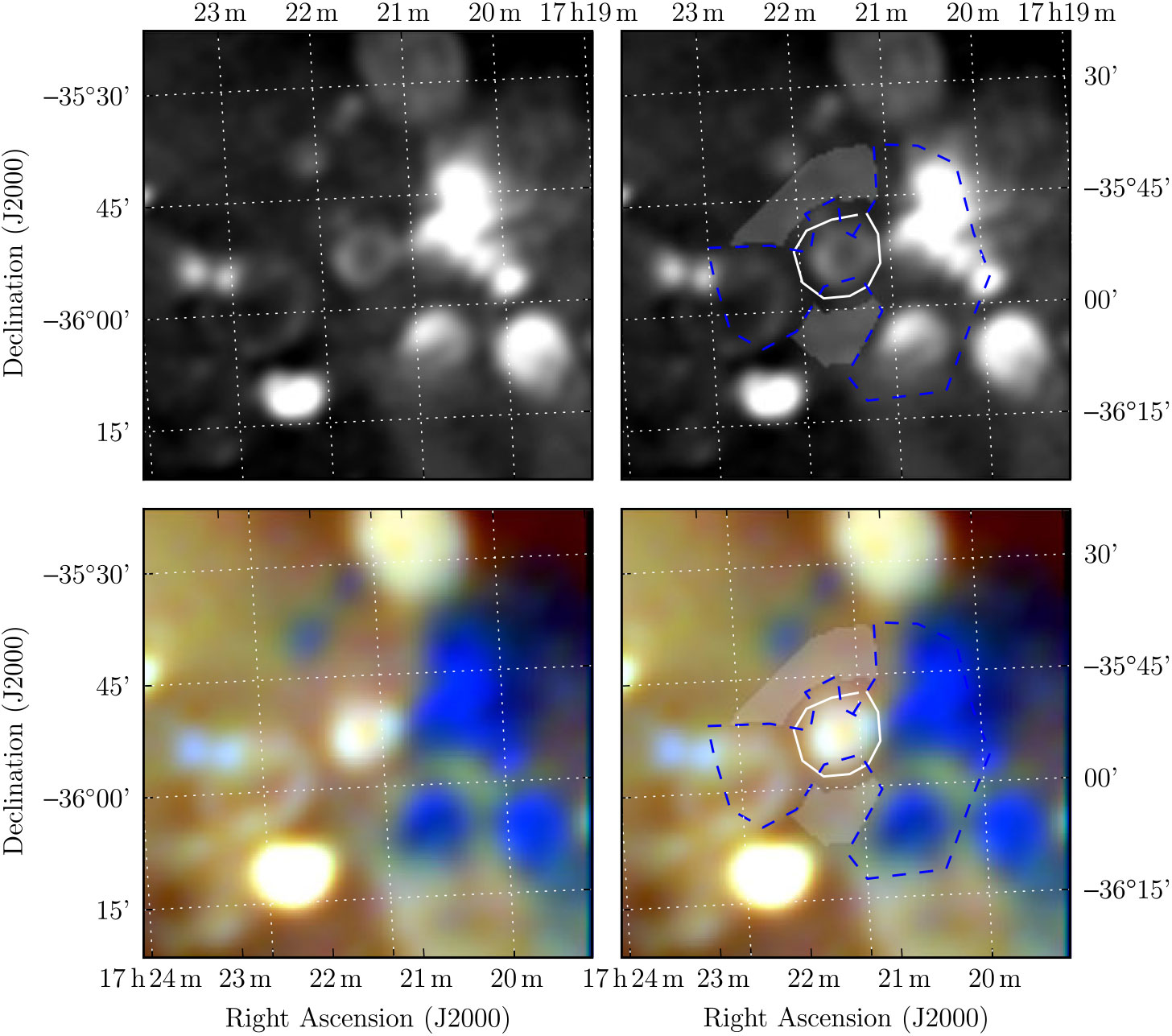
G 351.4 + 0.4 as imaged, detected, and measured in Paper II, demonstrating the method used in that paper and this work. The top two panels show the GLEAM 170–231 MHz images; the lower two panels show the RGB cube formed of the 72–103 MHz (R), 103–134 MHz (G), and 139–170 MHz (B) images. G 351.4 + 0.4 can be clearly discriminated as a white ellipse in the centre of the image, compared to the H ii regions surrounding it, which appear dark blue, due to their absorbing effect on the lowest frequency radio emission. The left two panels show the panels without annotation, while the right two panels show the use of the Polygon_Flux software. The white lines indicate polygons drawn to encapsulate the SNR shell measured in this work; the blue dashed lines indicate polygons drawn to exclude regions from being used as background; the grey shading indicates areas used to calculate the background.
2.4. Measuring SNRs
To effectively measure the flux densities of SNRs, we employed the Polygon_FluxFootnote l software (Hurley-Walker, in prep.). This presents an interactive view of the wide and RGB images, and allows the user to draw a polygon surrounding the object of interest. The user may also draw a polygon to encapsulate any regions which are thought to be contaminated with other objects which might interfere with a measurement of the background.
Once the polygons are selected, the flux densities of the SNR can be calculated from each of the 24 GLEAM mosaics, each convolved to the same resolution as the lowest-resolution image at 72–80 MHz. A background is calculated from an annulus surrounding the first polygon, excluding any regions selected by the second polygon. The total flux density inside the polygon is calculated and the average background level subtracted. This ensures that regardless of where the polygon is drawn, the total flux density of the SNR is calculated accurately. Figure 1 shows an example of the polygon drawing method.
Some larger SNRs are seen to overlap with point sources (see e.g. Section 3.1.5). A compact source near the centre of an SNR may be a pulsar or pulsar wind nebula (PWNe), but if it is off-centre, the origin is less clear. Extragalactic sources such as radio galaxies are fairly isotropically distributed and have varying brightnesses. At the resolution of the GLEAM survey, only one-third of radio galaxies are at all resolved, with a size more than 10 % greater than the local PSF, and the majority have non-thermal spectra with median α ≈ − 0.8 ± 0.2 (Hurley-Walker et al. Reference Hurley-Walker2017)]. We therefore consider any non-central, unresolved source with a non-thermal spectrum to be a contaminating extragalactic radio source. We perform compact source-finding and fitting across the full GLEAM band as per Hurley-Walker et al. (Reference Hurley-Walker2019c), forcing the background level to match that of the surrounding SNR. Sources thus measured are then subtracted from the flux density measurements of the SNR.
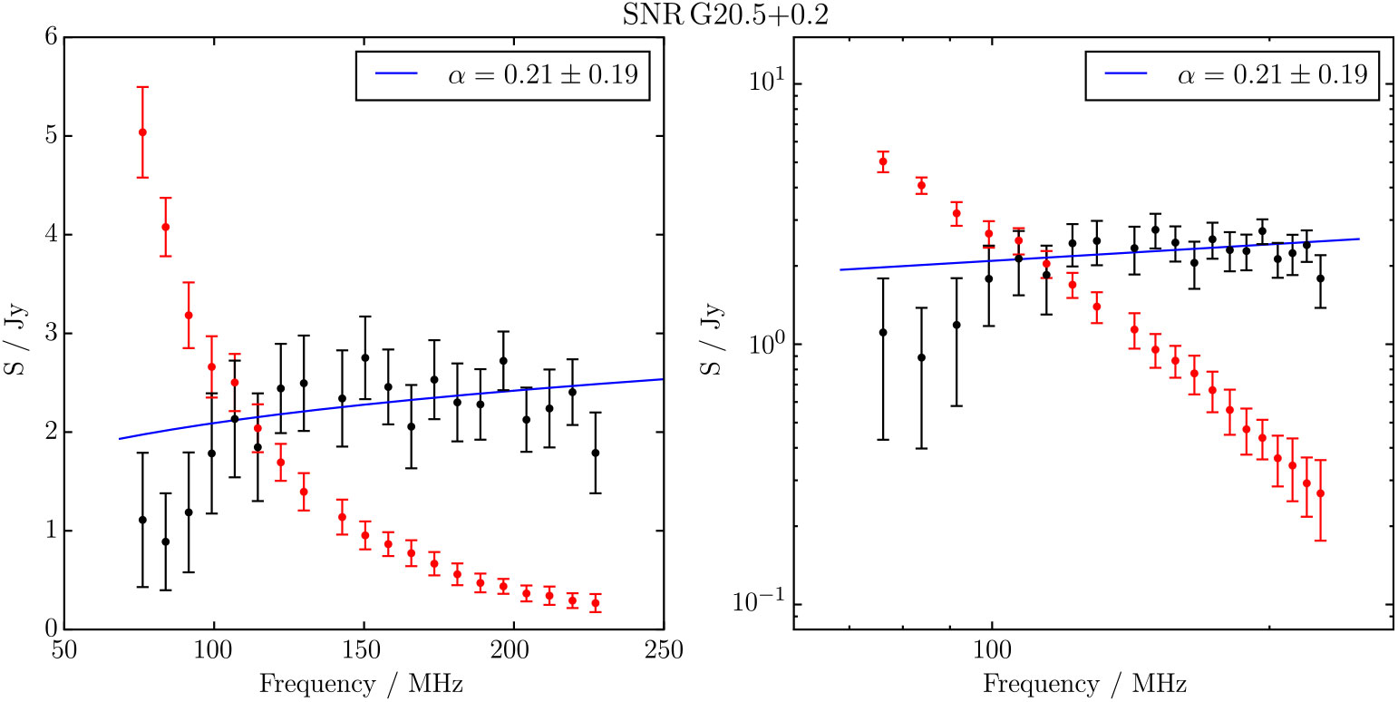
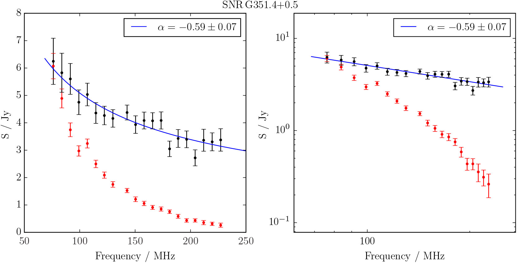
Once these flux densities are calculated, a power-law spectral energy distribution (SED) is fit to the spectra, using only the 20 narrow-band measurements. If the reduced χ 2 > 1.93, indicating a poor fit, the calculation is repeated for the wide-band images, to improve signal-to-noise. If that also shows a poor fit, no spectral index can be reported for that SNR. All calculations are saved to a FITS table for future use. Figure 2 shows an example of the output from the spectral fitting routine. Appendix B shows full details of the regions fit to the SNR images and Appendix C shows the resulting spectra for all objects measured in this work.
The spectrum of G 351.4 + 0.4 as measured using the backgrounding and flux summing technique described in Section 2.4. The left panel shows flux density against frequency with linear axes while the right panel shows the same data in log. (It is useful to include both when analysing the data as a log plot does not render negative data points, which occur for faint SNRs or negative background levels). The black points show the (background-subtracted) SNR flux density measurements, the red points show the measured background, and the blue curve shows a linear fit to the data above 150 MHz (marked in black) in log–log space (i.e. S ν ∝ ν α). The fitted value of α is shown at the top right.
For the new SNRs described in Paper II, the software is used to perform measurements in the MGPS and E11 datasets by using exactly the same polygons as determined when examining the GLEAM images. This allows us to avoid contamination from thermal regions and point sources in the object and background flux density measurements, and for partial objects, means the same fraction of the objects is measured. For the candidate SNRs in this work, published flux density measurements are often used in conjunction with the GLEAM measurements to derive SEDs, although on occasion using the same Polygon_Flux technique is useful.
2.5. SNR evolution
Multiple publications in the literature review the evolution of SNRs and suggest models of varying complexity to describe it. Given that from radio measurements alone, we generally know little about a given SNR aside from its radius, we restrict ourselves to modelling SNR evolution using the simplest descriptive models, following Woltjer (Reference Woltjer1972), and making standard assumptions about their energetics. Over the lifetime of an SNR, it passes through several stages, where relatively simple equations can be used to predict the SNR radius as a function of time (or estimate the SNR age, given its radius). The initial stage is the ejecta-dominated stage of free expansion, in which the radius R depends on velocity v and time t via:
 \begin{equation}R = v t.\end{equation}
The velocity of the ejecta depends on the energy of the SNR E and the ejecta mass M ejecta via (Woltjer Reference Woltjer1972):
 \begin{equation}v = \left(\frac{2E}{M_{\text{ejecta}}}\right) \approx 10^4\left(\frac{E}{10^{51}\text{erg}}\right)^{1/2}\left(\frac{M_{\text{ejecta}}}{M_\odot}\right)^{-1/2} \text{km s}^{-1}.\end{equation}
That is, 104 km s−1 for standard assumptions of M ejecta = M ȯ and E = 1051 erg.
As the ejecta collide with the ISM, a forward shock propagates outwards, and a reverse shock propagates toward the centre of the remnant. This adiabatic (or Sedov–Taylor) stage starts once mass of the swept-up ISM becomes comparable to the ejecta mass, at around 200 years for typical SNR, and the SNR is fully in this phase once the ejecta are fully thermalised. The SNR radius R is proportional to its age t via (Sedov Reference Sedov1959):
 \begin{equation}R=1.17\left(\frac{E}{\rho}\right)^{1/5}t^{2/5},\end{equation}
where ρ is the density of the surrounding ISM. Expressed in units typical of spherical SNRs expanding into the Galactic ISM:
 \begin{equation}R\approx5\left(\frac{E}{10^{51}\,\text{erg}}\right)^{1/5}\left(\frac{n_{\text{H}}}{\text{cm}^{-3}}\right)^{-1/5}\left(\frac{t}{1000\,\text{years}}\right)^{2/5}\,\text{pc}.
\end{equation}
\begin{equation}R\approx5\left(\frac{E}{10^{51}\,\text{erg}}\right)^{1/5}\left(\frac{n_{\text{H}}}{\text{cm}^{-3}}\right)^{-1/5}\left(\frac{t}{1000\,\text{years}}\right)^{2/5}\,\text{pc}.
\end{equation}
The SNR enters its third phase of radiative expansion, and the shocked ISM begins to cool, starting when the SNR is ≈ 50 000 years old, and the shell velocity is around 200 km s−1. The SNR is driven only by internal pressure instead of the initial kinetic expansion, and its radius R increases as t 2/7. Finally, the SNR cools and enters a stage where momentum drives the shell expansion, and eventually the shell velocity drops to the general ISM random values of ≈ 10 km s−1, and the SNR becomes indistinguishable from the surrounding ISM.
3. Results
We searched 101 non-MAGPIS candidate SNR positions and 18 MAGPIS candidate SNR positions (see Section 2.2) to identify regions where the GLEAM data could serve as a useful discriminant. In the first category, we identified 19 regions, presented in Section 3.1; in the second, we identified seven, discussed in Section 3.2.
3.1. Candidate SNRs
In this section we examine the 19-candidate SNR with useful GLEAM detections and compare to previous results in the literature, in order of Galactic longitude, first for the outer-Galactic ‘oG’ region (180° < l < 240°) and then the inner-Galactic ‘iG’ region (345° < l < 60°). Table 1 summarises the vital properties of these objects.
Summary of non-MAGPIS candidates, detailed in Section 3.1. Entries marked with a ‘*’, and all entries in rows or columns so marked, were derived in this work. Italics indicate candidates that we believe should no longer be considered potential SNRs. The flux density and spectral index for G 353.3-1.1 were calculated after the subtraction of contaminating radio sources, and extrapolation of the full shell morphology (see Section 3.1.6). The two objects classed with ‘SNR?’ are potentially SNRs but cannot be definitively proved so by this work. The object classed ‘Both’ is a composite thermal and non-thermal source, the former a H ii region and the latter either a compact SNR or a pulsar.

3.1.1 G189.6 + 3.3
G189.6 + 3.3 was detected by Asaoka & Aschenbach (Reference Asaoka and Aschenbach1994) as a faint X-ray excess overlapping G189.1 + 3.0 (IC443). Leahy (Reference Leahy2004) performed a detailed radio continuum mapping of the region and noted the presence of a radio-bright arc coincident with the northern edge of the SNR candidate proposed by Asaoka & Aschenbach (Reference Asaoka and Aschenbach1994), with a radio spectral index of α = −0.1– − 0.6. Lee et al. (Reference Lee, Koo, Yun, Stanimirović, Heiles and Heyer2008) used the VLA and Arecibo to investigate IC443 at 1 420 MHz and detected the arc of G189.6 + 3.3 where it intersects IC443. Our observations show about half of the shell that is visible in the X-ray observations. We were unable to extract a spectrum for the SNR candidate due to low signal-to-noise, and confusing effects from IC443. However, the peak flux density where the shell of G189.6 + 3.3 intersects with IC443, at RA = 6h 18m 30s, Dec = +22d50m, can be measured both our own data, and that of Lee et al. (Reference Lee, Koo, Yun, Stanimirović, Heiles and Heyer2008), who determine it to be ≈ 6 mJy beam−1 at 1420 MHz (Figure 3 of Lee et al. 2008) [c/f ≈ 1 K or ≈ 15 mJy beam−1 by Leahy (Reference Leahy2004)].
G189.6 + 3.3 as observed by ROSAT (left) and GLEAM at 200 MHz (right, including colour bar). The ROSAT X-ray image has been convolved with a Gaussian kernel 10 pixels wide in order to highlight the large-scale structure of SNR G189.6 + 3.3, which is marked with a dotted white ellipse. The dashed line in the right panel indicates the radio excess discussed in Section 3.1.1. The right panel also contains five logarithmically spaced thin black contours with levels between 0.3 and 10 Jy beam−1, inclusive, to highlight SNR IC 433.
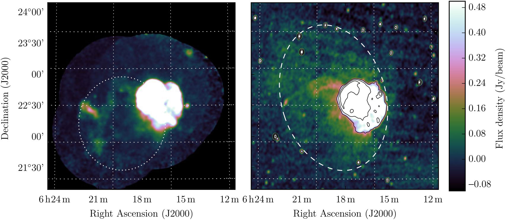
In our data, we first measure a background level of 60 mJy beam−1, from a nearby region not associated with either G 189.6 + 3.3 or IC443. Our peak flux density measurement at the above RA and Dec is 230 mJy beam−1, and 170 mJy beam−1 after background subtraction. Combining S 200 MHz = 170 mJy beam−1 and S 1.4GHz = 10 mJy beam−1, and assuming 30 % errors on each, yield a spectral index of α = −1.2 ± 0.2, consistent with an aged population of synchrotron-emitting electrons.
We note that this 60 mJy beam−1 background level seems to be associated with an elliptical radio excess, with a centre at RA = 6h 18m50s, Dec = +22d38m, diameter 2.4° × 1.8°, and a position angle of 20° (CCW from North), shown as a dashed ellipse in Figure 3. The RMS noise at 200 MHz in this region is about 20 mJy beam−1, but while the peak is low signal-to-noise, the total flux density is significant. In the lower-frequency wideband GLEAM images, the background flux density and RMS noise values in this area are 215, 90 mJy beam−1 (72–103 MHz), 100, 40 mJy beam−1 (103–134 MHz), and 68, 25 mJy beam−1 (139–170 MHz). A spectral fit to these background levels (using the RMS values as errors) gives a α = −1.5 ± 0.6, making this object potentially another candidate SNR. Sidelobes from inadequate calibration and deconvolution of the nearby Crab nebula increase the noise in the region; a more definitive statement could be made with more data processed to a higher quality.
3.1.2. G345.1– 0.2
Whiteoak and Green (Reference Whiteoak and Green1996) presented 18 new SNRs and 16 candidate SNRs found in observations by the MOST at 843 MHz. G345.1 – 0.2 falls into the candidate category and was described as a ‘bright shell with point source’, a diameter of 6 × 6 arcmin, a total flux density of 1.8 Jy, and a mean surface brightness of 7.1 × 10⁻²¹ W m−2Hz−1sr−1. Figure 4 shows the MGPS 843 MHz observation of G 345.1 – 0.2 and the corresponding GLEAM image at 200 MHz.
G345.1 – 0.2 as observed by MGPS at 843 MHz (left), GLEAM at 200 MHz (middle), and WISE (right).
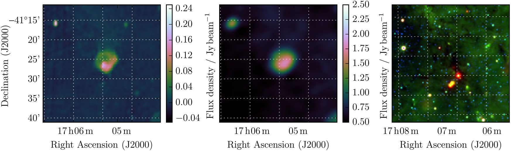
Despite the absence of any obvious emission in the WISE 12- and 22-μm maps of this area, there is some evidence of a low-frequency turnover within the GLEAM band (Figure A18). To avoid the effects of H ii region absorption on our spectral calculation, we use only those measurements with ν > 150 MHz, and include the measurement of Whiteoak and Green (Reference Whiteoak and Green1996) of S 843 MHz = 1.8 Jy, and find that the candidate has a slightly falling spectrum of α = −0.69 ± 0.06 and a fitted flux density of S 200 MHz = 4.30 ± 0.09 Jy. Its morphology and spectrum suggest that it truly is an SNR.
3.1.3. G345.1 + 0.2
Similar to G 345.1 – 0.2 (Section 3.1.2), G345.1 + 0.2 was also classed as a potential SNR by Whiteoak and Green (Reference Whiteoak and Green1996), who gave its properties as total flux density of 0.7 Jy, a 10 × 10 arcmin diameter, and a mean surface brightness of 0.7 × 10⁻²¹ W m−2Hz−1sr−1, describing it as ‘a faint shell’. Figure 5 shows the MGPS 843 MHz observation of G 345.1 + 0.2, and the corresponding GLEAM image at 200 MHz.
G345.1 + 0.2 as observed by MGPS at 843 MHz (left) and GLEAM at 200 MHz (right).
We tentatively confirm this morphology, noting that the shell appears to have a gap in the north-west. Background-subtracting our 200-MHz image and the 843-MHz MGPS image, and convolving the latter to the resolution of the former, we can form a spectral index map of the candidate. The shell has a spectral index of − 0.8 to − 0.4, while the source south-east of the shell has a flat spectrum of − 0.05. This source does not appear to have a counterpart in WISE, so is not a typical H ii region. It is difficult to separate the source from the shell at frequencies <200 MHz in GLEAM due to the low resolution of the survey, and the background level in GLEAM is similar to the total flux density of the candidate, so the uncertainties on our narrow-band measurements are large. We therefore suggest using the combined GLEAM and MGPS measurement as the most reliable estimator of its radio flux density and spectral index, calculating S 200 MHz = 1.6 ± 0.2 Jy and α = −0.57 ± 0.10.
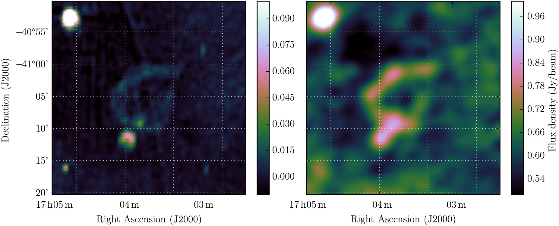
3.1.4. G348.8 + 1.1
Concluding our selection from Whiteoak and Green (Reference Whiteoak and Green1996) (see also Sections 3.1.2 and 3.1.3), G348.8 + 1.1 is a ‘category C’ candidate, which described only as a ‘faint, incomplete shell’ with 10 arcmin diameter, S 843 MHz = 0.1 Jy, and a mean surface brightness of 0.1 × 10⁻²¹ W m−2Hz−1sr−1. Figure 6 shows the MGPS 843 MHz observation of G348.8 + 1.1, and the corresponding GLEAM image at 200 MHz.
G348.8 + 1.1 as observed by MOST at 843 MHz (left) and GLEAM at 200 MHz (right).
Our observations do not clearly show the same shell-like structure, but find regions of increased brightness coincident with the NW SE, S, and central filaments seen in the MOST image. From our measurements we derive α = −0.7 ± 0.2 and S 200 MHz = 1.8 ± 0.2 Jy. However, these values are inconsistent with those listed by Whiteoak and Green (Reference Whiteoak and Green1996) in Table MSC.C; extrapolating to 843 MHz, we would expect to see ≈ 0.64 Jy of total flux density, instead of the listed 0.1 Jy. However, if we use our own Polygon_Flux software to measure the flux density in the MOST data, we find that the total flux density at 843 MHz is 0.7 Jy, consistent with our own observations, and thus suggest that Whiteoak & Green may have made a typographical error in their table. Given the existence in GLEAM, and spectrum of the candidate, we confirm it as an SNR.
PSR J1710-37 lies outside of the shell of G348.8 + 1.1 by more than its radius, so is unlikely to be associated.
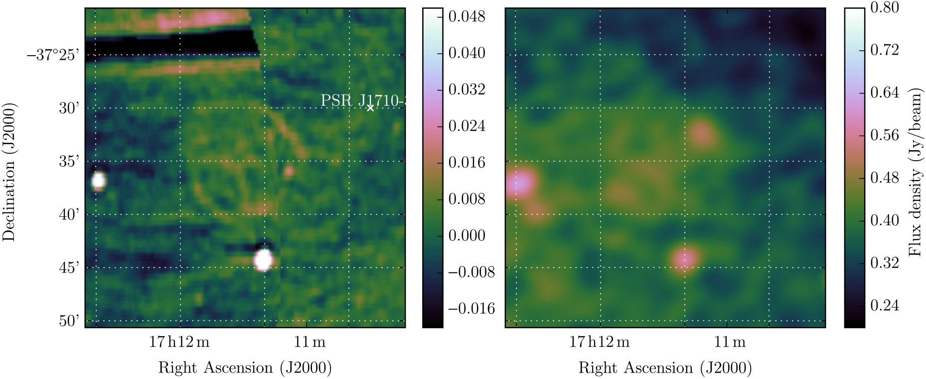
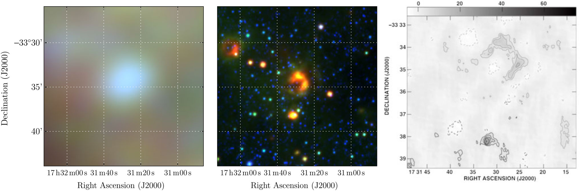
3.1.5. G352.2 – 0.1
Manchester et al. (Reference Manchester, Slane and Gaensler2002) used the Australia Telescope Compact Array and the MGPS to search for SNR associated with pulsars detected in the Parkes Multibeam Survey, in this case PSR J1726-3530. Figure 7 shows the MGPS 843 MHz observation of G352.2 – 0.1, and the RGB GLEAM cube at 72–103 MHz (R), 103–134 MHz (G), and 139–170 MHz (B). Our image shows strong absorption at 72–103 MHz, indicating the presence of H ii regions. However, the candidate does appear to have a shell-like shape, indicating it could well be an SNR.
G352.2 – 0.1 as observed by MOST at 843 MHz (left) and GLEAM at 72–103 MHz (R), 103–134 MHz (G), and 139–170 MHz (B) (right). The (linear) scales for the colour ranges of these frequencies are 4.0–7.0, 2.3–3.6, and 1.0–1.7 Jy beam−1, respectively.
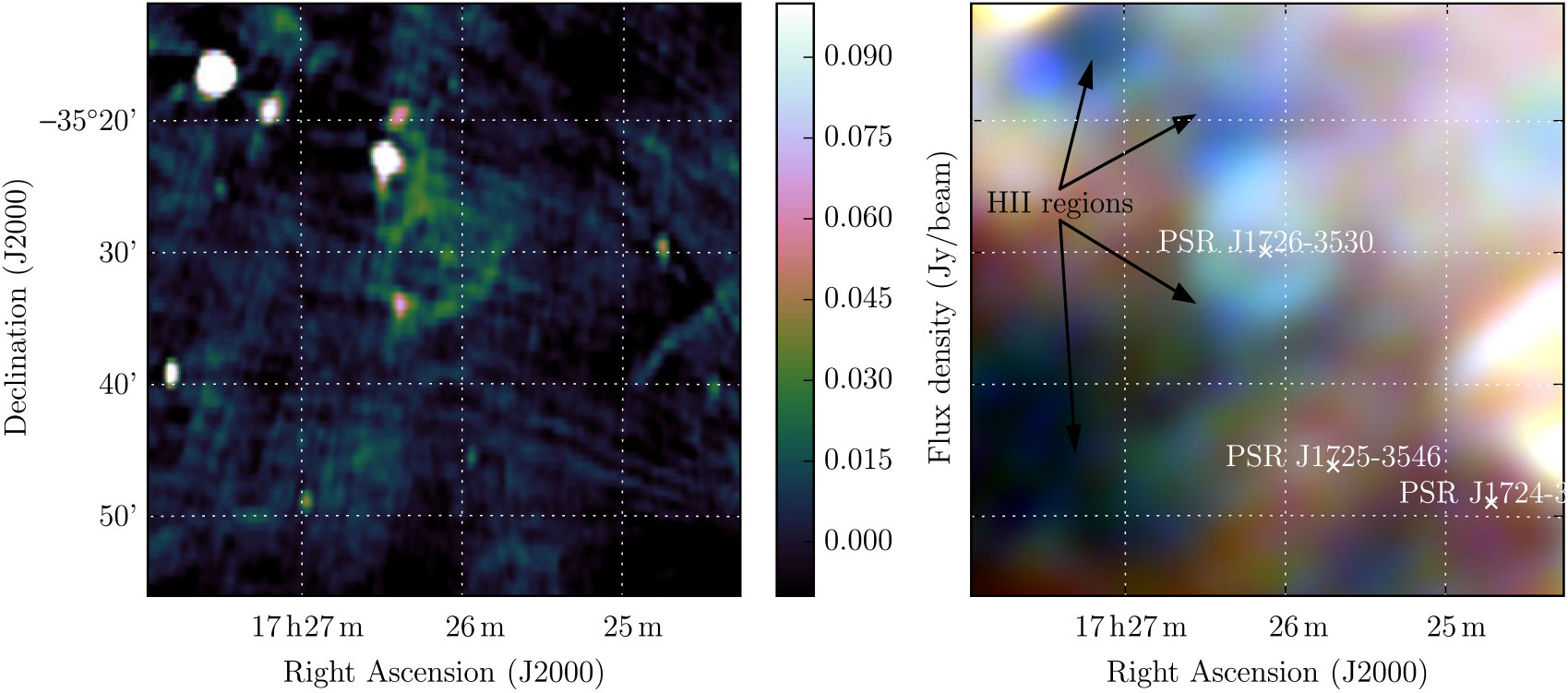
WISE shows increased 12- and 22-μm emission just northeast of the edge of this shell, corresponding to one of the most highly absorbing regions in our image. This region is sufficiently complex that we cannot derive a spectrum for the candidate, only the foreground H ii regions (see Figure A21). We estimate S 200 MHz = 2.0 ± 0.2 Jy without any correction for contaminating H ii regions. Using Polygon_Flux, we measure S 843 MHz = 1.3 ± 0.2 Jy from MGPS, deriving α = −0.30 ± 0.05 from these two measurements alone.
Using the pulsar dispersion measure (DM) of 718 cm–3 pc (Petroff et al. Reference Petroff, Keith, Johnston, van Straten and Shannon2013) and the electron density model of Yao et al. (Reference Yao, Manchester and Wang2017), a distance of 4.7 kpc can be assigned to PSR J1726-3530.Footnote m If PSR J1726-3530 and G352.2 – 0.1 are associated and there is no line-of-sight difference in distances, the SNR is 8 pc in diameter. PSR J1726-3530 has P ≈ 1.11 s and $\dot{P}\approx1.2\times10^{-12}\;{\rm s}\; {\rm s}^{-1}$
(Manchester et al. Reference Manchester2001), giving it a characteristic age of 14 500 years, in which it is likely to be in the Sedov–Taylor phase, described by Equation (4).
$\dot{P}\approx1.2\times10^{-12}\;{\rm s}\; {\rm s}^{-1}$
(Manchester et al. Reference Manchester2001), giving it a characteristic age of 14 500 years, in which it is likely to be in the Sedov–Taylor phase, described by Equation (4).
After 14 500 years, a typical SNR in this phase would therefore be ≈ 29 pc in diameter, more than three times larger than the observed diameter. There are multiple factors which could cause such an inconsistency: the distance estimate may yet be wrong (having already been revised by a factor of two in a decade); the SNR may have an unusually (≈ 530×) low energy (unlikely to be the sole factor given SNR energies range from 1050 to 1052 erg; see Leahy Reference Leahy2017); or the ISM may be overdense by a similar factor. Additionally, pulsar characteristic ages are usually an overestimate since they assume a spindown from P = 0 (see e.g. Kaspi et al. Reference Kaspi, Roberts, Vasisht, Gotthelf, Pivovarof and Kawai2001), but not usually by the necessary factor of ≈ 20, particularly for a slow pulsar such as PSR J1726-3530. We cannot easily reconcile these values and suggest some combination of factors would be necessary to explain the discrepancy. Given the known pulsar spatial density in the region, there is also a ≈ 40 % chance that the pulsar lies within the shell of the SNR purely through chance geometrical alignment.
3.1.6. G353.3 – 1.1
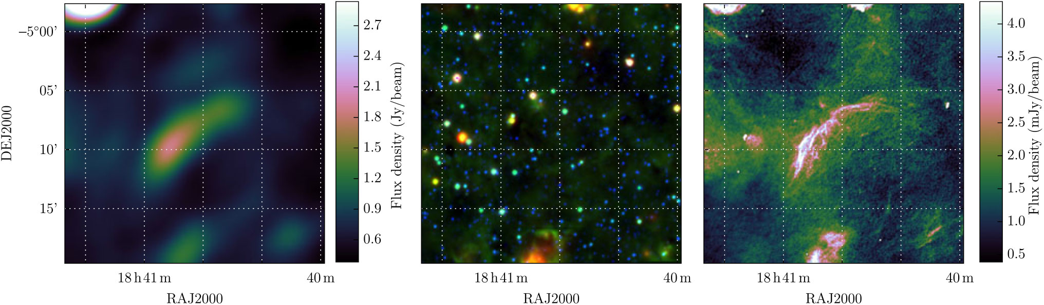
Using the Parkes radio telescope at 2.4 GHz, Duncan et al. (Reference Duncan, Stewart, Haynes and Jones1995) conducted a survey of the Galactic plane in continuum and polarisation, publishing 25 SNR candidates (Duncan et al. Reference Duncan, Stewart, Haynes and Jones1997). Many of these have since been confirmed as SNRs, but the large angular diameter (≈ 1°) and partial, poorly resolved morphology of G353.3 – 1.1 has made it difficult to confirm. Figure 8 shows the Parkes 2.4 GHz continuum image of G353.3 – 1.1 and the GLEAM RGB cube of the same region.
G353.3 – 1.1 as observed by Parkes at 2.4 GHz (left) and GLEAM at 72–103 MHz (R), 103–134 MHz (G), and 139–170 MHz (B) (right). All frequencies are set to an identical linear colour scale of 0.5–5.0 Jy beam−1
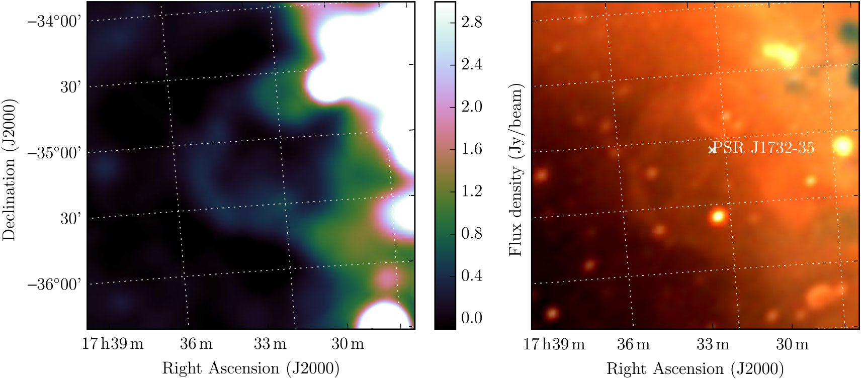
The GLEAM observations confirm this object as an SNR, clearly resolving the shell structure against the diffuse Galactic background and despite the presence of other SNRs and contaminating extragalactic radio sources. Given that half of the shell is obscured by other SNRs, we use Polygon_Flux to measure half of the shell (Figure A5). We also use Polygon_Flux to measure G353.3 – 1.1 in the Parkes 2.4 GHz continuum image,Footnote n across the same region fitted in GLEAM. To deal with the contaminating compact radio sources, we performed compact source-finding and fitting across the full GLEAM band as per Hurley-Walker et al. (Reference Hurley-Walker2019c), finding six unresolved sources with S 200 MHz > 5 × the local RMS noise. In total, these had S 200 MHz = 6.3 Jy and a median α = −0.84.
We extrapolate the radio source spectra across 72–2.4 GHz and subtract them from all measurements. Two of the sources have flat or rising spectra with large error bars, so we do not extrapolate these to 2.4 GHz. There is some evidence for contamination by H ii regions in the spectrum, as it begins to flatten at ν < 150 MHz. We therefore fit to the source-subtracted data for ν > 150 MHz, resulting in α = −0.85 ± 0.04 and S 200 MHz = 43 ± 4 Jy (Figure A22). Since we are measuring approximately half of the shell, we postulate that the total flux density is 95 ± 8 Jy.
One pulsar lies 10'.5 from the centre of the shell: Ng et al. (Reference Ng2015) detected PSR J1732-35 using the Parkes radio telescope at 1.4 GHz as part of the High Time Resolution Universe (HTRU) survey. The pulsar has a spin period of P ≈ 127 ms, a DM of 340 ± 2 cm−3 pc, and therefore a distance of 4.1 kpc (Yao et al. Reference Yao, Manchester and Wang2017).Footnote o Timing solutions are not yet precise enough to determine whether the pulsar is isolated or in a binary system, so it is not possible to tell if this spin rate is due to partial recycling or simply youth. The period derivative of the pulsar has not yet been measured, so an age cannot be estimated. However, if $\dot{P}\gtrsim 10^{-13}{\rm s}\;{\rm s}^{-1}$
, its P and
$\dot{P}\gtrsim 10^{-13}{\rm s}\;{\rm s}^{-1}$
, its P and $\dot{P}$
would be typical of pulsars with SNR associations.
$\dot{P}$
would be typical of pulsars with SNR associations.
If the pulsar distance estimate is correct and the pulsar and SNR are associated, G353.3 – 1.1 is 71 pc in diameter, and the pulsar has moved 12 pc since birth. Reversing Equation (4), we can use the SNR radius to predict the age, finding t ≈ 130 000 yr. At this age the SNR is not likely to still be in the Sedov–Taylor phase, and is likely in the ‘snow plough’ stage, where its radius will evolve more slowly with respect to time (R ∝ t 2/7). This age could therefore be considered a lower limit. The pulsar line-of-sight velocity would therefore be <90 km s−1, reasonable considering that 32 % of young pulsars have velocities distributed in a Maxwellian with an average velocity of $\sigma\sqrt{8/\pi}=130\; {\rm km}\; {\rm s}^{-1}$
(Verbunt et al. Reference Verbunt, Igoshev and Cator2017). Given the pulsar spatial density in this region and the large size of the shell, we would expect at least one pulsar to lie within the shell purely through geometric coincidence. A measurement of the pulsar’s
$\dot{P}$
or true velocity would help to confirm its association with the SNR.
$\sigma\sqrt{8/\pi}=130\; {\rm km}\; {\rm s}^{-1}$
(Verbunt et al. Reference Verbunt, Igoshev and Cator2017). Given the pulsar spatial density in this region and the large size of the shell, we would expect at least one pulsar to lie within the shell purely through geometric coincidence. A measurement of the pulsar’s
$\dot{P}$
or true velocity would help to confirm its association with the SNR.
3.1.7. G354.46 + 0.07
Roy & Pal (Reference Roy and Pal2013) used the GMRT to observe G354.46 + 0.07 at 330 MHz and 1.4 GHz. They made long-baseline and short-baseline images in order to separate extended (>2 arcmin) H ii region emission from what they identified as a young SNR shell. They attributed to the ‘shell’ flux densities of S 300 MHz = 0.9 ± 0.1 Jy and S 1400 MHz = 0.7 ± 0.1 Jy, and thereby determined a spectral index of α = −0.2 ± 0.1, which they note is ‘quite flat and unexpected for a shell-type SNR’. We also note that in Figure 3, they plot these flux densities multiplied by a factor of four, but have not concomitantly multiplied the error bars.
Searching the WISE data, we find that this ‘shell’ has the same morphology as a 12- and 22-μm emitting region, strongly indicating it is actually an H ii region. Our GLEAM observations would not be able to resolve the shell were it to be present, but they do show that there is no emission on a 4’-scale, which is what Roy & Pal (Reference Roy and Pal2013) claim as the extent of the H ii region. Figure 9 shows the WISE, GLEAM, and GMRT high-resolution data for this region, while Figure A23 shows the GLEAM spectrum, with a distinct low-frequency turnover indicating absorption of Galactic synchrotron from an H ii region. We argue that G354.5 + 0.1 has been mistakenly identified as an SNR and is in fact an H ii region.
G354.5 + 0.1 as observed by GLEAM (left) at 72–103 MHz (R), 103–134 MHz (G), and 139–170 MHz (B), by WISE (middle) at 22 μm (R), 12 μm (G), and 4.6 μm (B), and with the GMRT at 1.4 GHz with (u, v) > 1000λ (left panel of Figure 2 from Roy & Pal 2013). The colour scales for the GLEAM RGB cube are 4.3–8.6, 2.0–4.4, and 0.8–2.3 Jy beam−1, respectively.
3.1.8. G356.6 + 0.1
Gray (Reference Gray1994) searched the Galactic Centre using the MOST and detected 24-candidate SNR, many of which are not visible in the GLEAM images, in many cases because the Galactic Centre is such a complex region that disentangling individual objects becomes difficult. Gray identify G 356.6 + 0.1 and suggest S 843 MHz = 3.7 Jy, although with ‘much uncertainty’. WISE shows a small circular region of increased 22-μm emission to the south-west of the object, which is likely an H ii region. This is also noted by Gray as IRAS 17335 − 3136. The GLEAM observations do not resolve the source into the two components, but the GLEAM RGB image (Figure 10) shows that it has a flatter spectrum toward the southwest, consistent with this part being a H ii region. Running Polygon_Flux on MGPS data, we can separate the object into the likely H ii region component and the potential shell component, finding S 843MHz,H ii = 0.72 ± 0.7 Jy and S 843MHz,shell = 0.37 ± 0.4 Jy. Assuming the H ii region has a flat spectrum of α = 0.0, we can subtract the first value from all GLEAM flux density measurements. Restricting the fit to ν > 150 MHz to avoid any absorbing effect from the H ii region, we find S 200 MHz = 1.9 ± 0.3 Jy and α = −1.1 ± 0.3, distinctly non-thermal. However, this analysis assumes that the MGPS data and our Polygon_Flux measurement is superior to that of Gray (Reference Gray1994), and they overestimated the 843-MHz flux density by a factor of ≈2.
G356.6 + 0.1 as observed by GLEAM (left) at 72–103 MHz (R), 103–134 MHz (G), and 139–170 MHz (B), by WISE (middle) at 22 μm (R), 12 μm (G), and 4.6 μm (B), and with MGPS at 843 MHz (right). The colour scales for the GLEAM RGB cube are all 2–10 Jy.
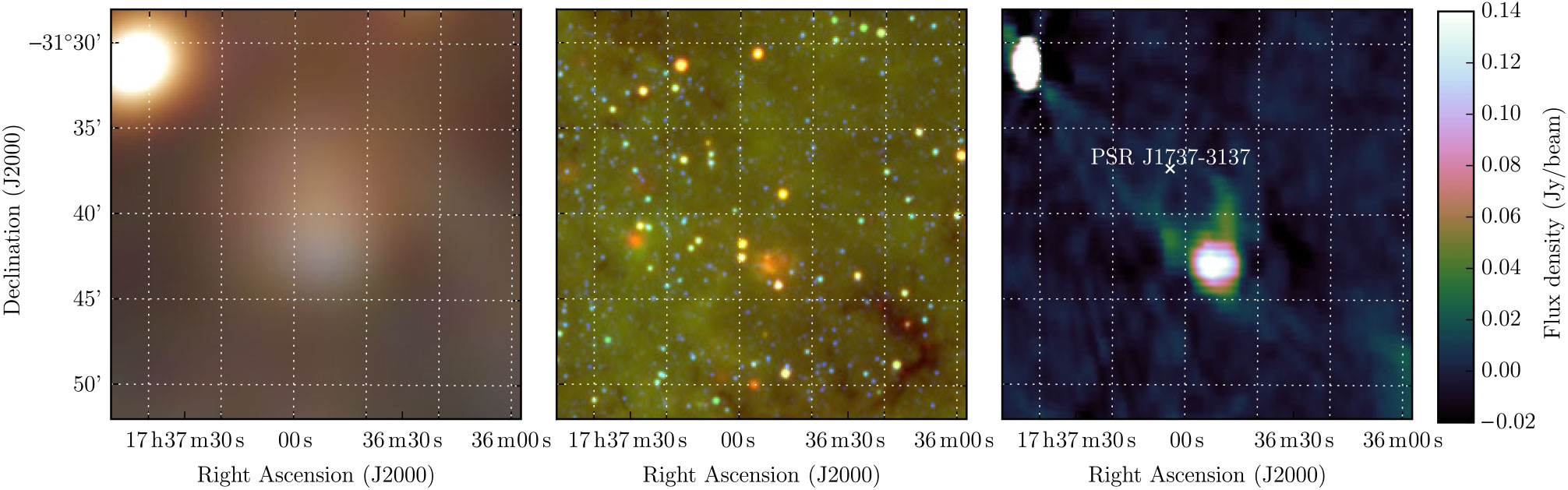
PSR J1737-3137 lies just on the edge of the shell (Figure 10) and has P ≈ 450 ms and $\dot{P}\approx1.4\times10^{-13}\; {\rm s}\; {\rm s}^{-1}$
(Morris et al. Reference Morris2002), giving it a characteristic age of ≈ 51,000 years. If it is associated with the SNR, then its distance of 4.2 kpc (Yao et al. Reference Yao, Manchester and Wang2017) would constrain the SNR to be 9 pc in diameter. Equation (4) predicts a radius of 24 pc for an SNR of this age, that is, about five times larger than expected if the pulsar association is correct. The factors in Section 3.1.5 would have to be even more extreme in order to explain this discrepancy, so we suspect the SNR and pulsar are not related, despite the low probability (≈3 %) that the pulsar and SNR are geometrically aligned by chance.
$\dot{P}\approx1.4\times10^{-13}\; {\rm s}\; {\rm s}^{-1}$
(Morris et al. Reference Morris2002), giving it a characteristic age of ≈ 51,000 years. If it is associated with the SNR, then its distance of 4.2 kpc (Yao et al. Reference Yao, Manchester and Wang2017) would constrain the SNR to be 9 pc in diameter. Equation (4) predicts a radius of 24 pc for an SNR of this age, that is, about five times larger than expected if the pulsar association is correct. The factors in Section 3.1.5 would have to be even more extreme in order to explain this discrepancy, so we suspect the SNR and pulsar are not related, despite the low probability (≈3 %) that the pulsar and SNR are geometrically aligned by chance.
3.1.9. G359.2 – 1.1
SNR G359.2 – 1.1 is a candidate detected by Gray (Reference Gray1994), and its higher Galactic latitude makes easier to distinguish, although at 4 × 5 arcmin it is close to unresolved by GLEAM. Gray describe it as asymmetric, and note that its lack of sharp edges potentially makes it less likely to be an SNR. ‘With considerable uncertainty’, they estimate S 843 MHz = 1.3 Jy. Using Polygon_Flux on the MGPS data, we find S 843 MHz = 0.56 Jy. Gray note the lack of IR emission from IRAS; in WISE there is no obvious diffuse 12- or 22-μm emission. PSR J1748-3009 lies nearby but with a period of P ≈ 9 ms, it is likely an unrelated recycled pulsar (
$\dot{P}$
has not yet been measured). Figure 11 displays the GLEAM, WISE, and MGPS images for this region.
G359.2 – 1.1 as observed by GLEAM (left) at 72–103 MHz (R), 103–134 MHz (G), and 139–170 MHz (B), by WISE (middle) at 22 μm (R), 12 μm (G), and 4.6 μm (B), and with MGPS at 843 MHz. The colour scales for the GLEAM RGB cube are 7.1–19.7, 3.1–10.1, and 1.1–4.7 Jy beam−1 for R, G, and B, respectively.
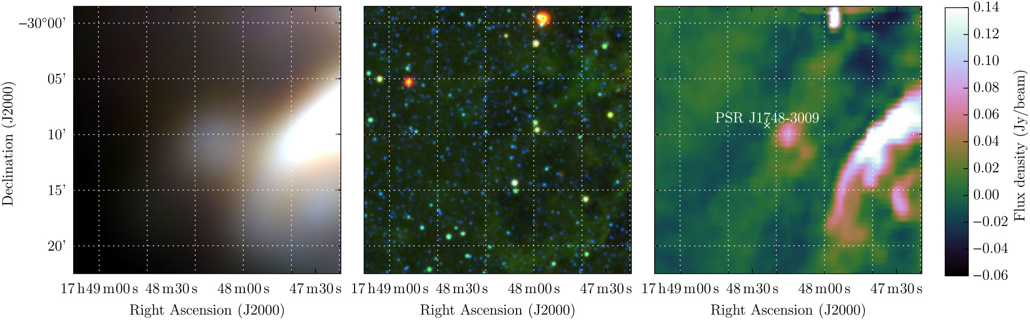
The GLEAM observations yield S 200 MHz = 2.6 ± 0.2 Jy and α = −0.83 ± 0.2, which would predict S 843 MHz = 0.8 Jy, slightly more consistent with our own measurement on MGPS than the measurement of Gray (Reference Gray1994) (similar to G356.6 + 0.1, Section 3.1.8). Given the low S/N of this source in both our data and the MGPS, we fit a single power-law SED to the GLEAM flux densities and our measurement from MGPS, and find S 200 MHz = 2.6 ± 0.2 and α = −1.07 ± 0.08, clearly non-thermal. Higher-resolution observations will be necessary to confirm the morphology, so we only tentatively confirm this candidate (Table 1).
3.1.10. G1.2 – 0.0
Sawada et al. (Reference Sawada, Tsujimoto, Koyama, Law, Tsuru and Hyodo2009) investigated the Sagittarius D H ii region with the Suzaku X-ray telescope. They identified ‘Diffuse Source 1’ (DS1) via its diffuse X-ray emission, and proposed it as a previously unknown SNR. They identified this also as a region of emission at 18 cm from observations made by Mehringer et al. (Reference Mehringer, Goss, Lis, Palmer and Menten1998). From 3.5 cm and 6.0 cm observations taken by Law et al. (Reference Law, Yusef-Zadeh, Cotton and Maddalena2008) with the GBT they calculated the spectral index of this emission to be α = −0.5.
However, GLEAM observations reveal this region to have large amounts of low-frequency absorption, and a rising spectrum, indicative of H ii regions. WISE images show 12- and 22-μm emission in the same location, also indicating a thermal origin to the radio emission. We argue that G1.2 – 0.0 has been mistakenly identified as an SNR and is in fact several superposed and complex H ii regions. Figure 12 shows the GLEAM and WISE data for this region, and a reproduction of Figure 6(a) from Sawada et al. (Reference Sawada, Tsujimoto, Koyama, Law, Tsuru and Hyodo2009).
G1.2 – 0.0 as observed by GLEAM (left) at 72–103 MHz (R), 103–134 MHz (G), and 139–170 MHz (B), by WISE (middle) at 22 μm (R), 12 μm (G), and 4.6 μm (B) and by Sawada et al. (Reference Sawada, Tsujimoto, Koyama, Law, Tsuru and Hyodo2009) with Suzaku X-ray (0.7–5.5 keV) in blue, Spitzer MIR (24 μm) in green, and GBT radio (6.0 cm) in red. The slice for the calculated radio spectral index (α = −0.5) is shown with a ticked vector. Objects are labelled in Italic for SNRs and in Roman for H ii regions. The colour scales for the GLEAM RGB cube are 11–38, 5–21, and 2–11 Jy beam-1 for R, G, and B, respectively.

3.1.11. G3.1 – 0.6
G 3.1 – 0.6 is the second-brightest object in the candidate sample of Gray (Reference Gray1994), with S 843 MHz = 6 Jy, and is described as being 28 × 52 arcmin, with ‘extensive filaments’. Roy and Rao (Reference Roy and Rao2002) used the GMRT at 330 MHz to follow up G3.1 – 0.6 and found similar filamentary structures. They also found increased emission toward the south-west of the region, and a potential shell-like structure in the southernmost part. We argue, however, that this is not a separate structure, and merely a chance of coincidence of filaments.
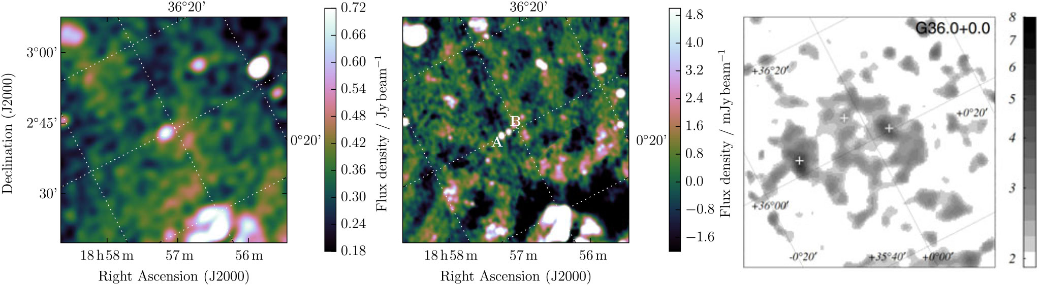
Figure 13 shows the MGPS 843 MHz observation of G3.1 – 0.6, the 200-MHz GLEAM image, and the RGB GLEAM cube at 72–103 MHz (R), 103–134 MHz (G), and 139–170 MHz (B). The MGPS data resolves out the large-scale structure of the region, and indeed only filamentary edges are visible. However, the GLEAM data show the large-scale structure of this candidate, and it is clear that the morphology is very complex, with two distinct regions: a spherical object ‘A’ centred at RA = 17h54m50s, and Dec = −26d39m30s, with radius 15 arcmin, and a more elliptical object ‘B’, which is consistent with a filled arc of equivalent radius 30 arcmin centred at the same position; these are marked in Figure 13. The ratio of flux densities between A and B is almost unity and its uncertainty is dominated by the subjective decision of how to separate the components. The chance of two short-lived SNR of such similar brightnesses and spectral indices (identical within errors) just happening to overlap along the line-of-sight is very small, so we believe these two structures are part of the same object.
G3.1 – 0.6 as observed by MGPS at 843 MHz (left), GLEAM at 200 MHz (middle), and at 72–103 MHz (R), 103–134 MHz (G), and 139–170 MHz (B) (right). The colour scales for the MGPS and GLEAM 200 MHz data are shown in the figure, while the colour scales for the GLEAM RGB cube are 4.8–13.2, 1.8–6.3, and 0.5–2.8 Jy beam−1 for R, G, and B, respectively. On the middle panel, we have overlaid a black ellipse (‘A’) and a white arc (‘B’) indicating the two potential expanding shells of different radii propagating from the same stellar explosion (see Section 3.1.11).
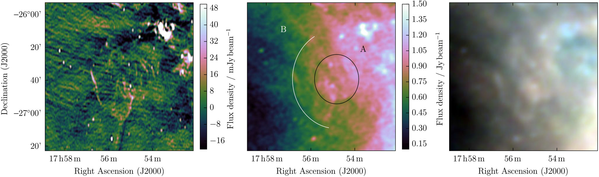
This SNR is reminiscent of the Cygnus Loop (e.g. Figure 1 of Leahy et al. Reference Leahy, Roger and Ballantyne1997), or, even more so, VRO42.05.01 (see right panel of Figure 2 of Leahy & Tian Reference Leahy and Tian2005). Landecker et al. (Reference Landecker, Pineault, Routledge and Vaneldik1982) examine this latter remnant in detail, concluding that its asymmetric morphology is most likely due to a single SNR expanding into two slabs of very different densities: the star explodes into a dense slab of gas, forming a circular shell; on the west side, the shock front breaks out of the dense slab and expands rapidly into a lower-density medium, forming a larger ‘wing’-like object, very similar to object ‘B’. Further interactions with denser regions of the ISM increase the brightness of the edge of the wing (see Pineault et al. Reference Pineault, Pritchet, Landecker, Routledge and Vaneldik1985; Reference Pineault, Landecker and Routledge1987, for further details). We postulate that G 3.1 – 0.6 is undergoing a similar type of expansion. Like Landecker et al. (Reference Landecker, Pineault, Routledge and Vaneldik1982), we may estimate the density discontinuity between the two slabs by assuming that the remnant is in the adiabatic phase and the SNR energy has been divided equally between the two components. The ratio of radii of the two components is 2:1, and the Sedov–Taylor relation (equation 3) implies $R_{\text{A}}^5\rho_{\text{A}} = R_{\text{B}}^5\rho_{\text{B}}$
. Therefore, the ρ A/ρ B ≈ 32.
$R_{\text{A}}^5\rho_{\text{A}} = R_{\text{B}}^5\rho_{\text{B}}$
. Therefore, the ρ A/ρ B ≈ 32.
Arias et al. 2019 postulate an alternative explanation for the shape of VRO42.05.01, where the progenitor star was moving at supersonic velocities from a high- to low-density environment, creating a bow-shock in the latter. After forming a supernova, the ‘wing’ expands outward into the bow-shock cavity, while the circular shell expands in the cavity left behind in the higher-density medium. In the case of G 3.1 – 0.6, the edge of the ‘wing’ appears more circular than triangular, and the MGPS image (left panel of Figure 13) shows filaments reconnecting the wing toward the centre of the explosion, which may be less compatible with a bow-shock interpretation. In any case, we cannot explain the morphology and non-thermal spectrum of the candidate by any mechanism other than an SNR and therefore confirm G 3.1 – 0.6 as an SNR.
3.1.12. G5.3 + 0.1
Trushkin (Reference Trushkin, Gimenez, Reglero and Winkler2001) searched NVSS data for polarised features which were part of shell-like objects in the continuum images, and followed them up with the RATAN-600 telescope at 0.96, 2.3, and 3.9 GHz. From these data they selected 15-candidate SNR, of which SNR G5.3 + 0.1 is one. We attempted to extract a spectrum for this SNR from the listed websiteFootnote p but found it was not available. Trushkin (Reference Trushkin, Gimenez, Reglero and Winkler2001) indicate that has size 2′.5 × 2′.0, and therefore nearly unresolved in GLEAM.
WISE shows a classic H ii region in this location, with strong central 22-μm emission, and an encircling ring of 12-μm emission. The GLEAM data show very strong absorption at low frequencies at this location. However, these features are ≈ 15 arcmin in size, and there is no sign of compact emission on a 2 arcmin scale. The NVSS image does have some compact features, but the quality is poor due to inadequate sampling and deconvolution of features on larger scales. We conclude that G5.3 + 0.1 is not an SNR, but part of a H ii region, only partly resolved by the VLA and RATAN-600. Figure 14 shows the GLEAM, WISE, and NVSS images for this region.
G5.3 + 0.1 as observed by GLEAM (left) at 72–103 MHz (R), 103–134 MHz (G), and 139–170 MHz (B), by WISE (middle) at 22 μm (R), 12 μm (G), and 4.6 μm (B) and NVSS at 1.4 GHz (right). The colour scales for the GLEAM RGB cube are 6.6–15.1, 3.4–7.8, and 1.3–3.5 Jy beam−1 for R, G, and B, respectively.
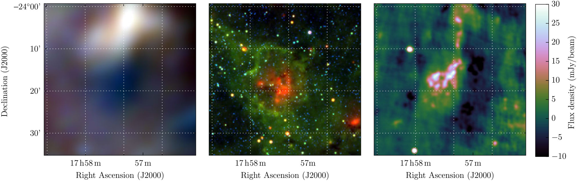
3.1.13. G 7.5 – 1.7
Roberts and Brogan (Reference Roberts and Brogan2008) observed G7.5 – 1.7 as an irregular shell surrounding the PWNe ‘Taz’, which itself is centred on the variable γ-ray source 3EG J1809-2328. Roberts & Brogan followed up the X-ray excess they observed in archival ROSAT and Advanced Satellite for Cosmology and Astrophysics (ASCA) data with a VLA observation at 324.84 MHz, and also used the Effelsberg Bonn 11-cm (2695 MHz) Survey (Reich et al. Reference Reich, Fuerst, Haslam, Steffen and Reif1984) to examine the emission in this region. They found evidence for a shell of radio emission with a steep (α ≈ − 0.8) spectral index. Figure 15 shows the röntgensatellit (ROSAT) Position-Sensitive Proportionate Counter (PSPC) 0.1–2.4 keV image, with 2695 MHz contours, and the GLEAM RGB cube of the same region.
G7.5 – 1.7 as observed by ROST PSPC at 0.1–2.4 keV (left), GLEAM at 72–103 MHz (R), 103–134 MHz (G), and 139–170 MHz (B) (middle), and by Effelsberg at 2695 MHz (right). The colour scales for the GLEAM RGB cube are 0.5–6.0, 0.1–3.5, and − 0.1–2.0 Jy beam−1 for R, G, and B, respectively.
GLEAM reveals the larger angular scales of this object quite clearly, showing a large irregular ellipse with an NW edge coincident with the steep-spectrum shell identified in Figure 3 of Roberts and Brogan (Reference Roberts and Brogan2008) (dashed arc on Figure 15). There is a faint inner circular ring in the GLEAM image, centred about 10’ to the East of ‘Taz’. This is reminiscent of the shape of extended PWNe such as the Crab Nebula (Figure 10 of Dubner et al. Reference Dubner, Castelletti, Kargaltsev, Pavlov, Bietenholz and Talavera2017), although more circular. We confirm G 7.5 – 1.7 as a Crab-like SNR with a shell.
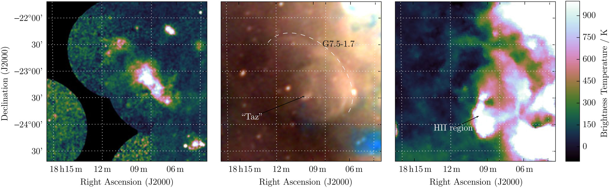
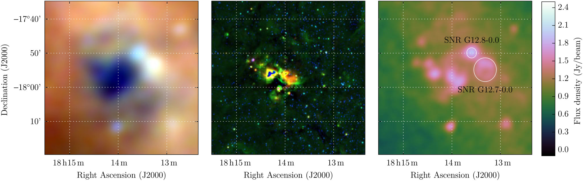
3.1.14. G12.75 – 0.15
Gosachinskii (Reference Gosachinskii1985) used publicly available radio surveys at 408 MHz (Shaver & Goss Reference Goss and Shaver1970), 1.42 GHz (Alferova et al. Reference Alferova, Venger, Gosachinskij, Kurochkina, Komar, Mogileva and Khersonskij1983), 4.875 GHz (Altenhoff et al. Reference Altenhoff, Downes, Pauls and Schraml1979), 5 GHz (Goss & Shaver Reference Goss and Shaver1970), and 10.7 GHz (MacLeod & Doherty Reference MacLeod and Doherty1968) to determine spectral indices of 14 extended Galactic sources, and suggested that the eight with non-thermal spectra may be SNRs. Of these eight, G12.75 – 0.15 was listed as having α = −0.61, and S 408 MHz = 53 ± 8 Jy, which would lead to S 200 MHz = 82 ± 12 Jy. With an angular extent of 15 arcmin, this should be overwhelmingly obvious in the GLEAM images.
Figure 16 shows an image of this region; the only feature on a 15 arcmin scale is an irregular H ii region of dimensions 15′ × 12′, clearly shown in absorption in the low frequencies of GLEAM (left panel), and in 12- and 22-μm emission in WISE (middle panel). Two known SNRs of diameters 3 and 6 arcmin are also labelled in the 200-MHz image (right panel) and appear unrelated to the H ii region. Gosachinskii (Reference Gosachinskii1985) fitted Gaussian templates to try to separate the Galactic background level from the observed features, and perhaps were unable to correctly separate thermal from non-thermal emission in this case. We suggest that G12.75 – 0.15 is not an SNR, but a H ii region.
G12.75 – 0.15 as observed by GLEAM (left) at 72–103 MHz (R), 103–134 MHz (G), and 139–170 MHz (B), by WISE (middle) at 22 μm (R), 12 μm (G), and 4.6 μm (B) and GLEAM at 200 MHz (right). The colour scales for the GLEAM RGB cube and wideband 200-MHz image are 1.9–8.0, 1.9–4.8, 1.2–2.7, and − 0.1–2.5 Jy beam−1, respectively.
3.1.15. G13.1 – 0.5
The Clark Lake (CL) survey of the Galactic plane at 30.9 MHz (Kassim Reference Kassim1988) was analysed by Gorham (Reference Gorham1990), who compared it with higher-frequency radio data in order to distinguish candidate SNR from H ii regions, which are seen in absorption at 30.9 MHz. The resolution of the CL survey was 11 × 13 arcmin with a sensitivity of 2 Jy, and many of these candidates have since been confirmed as true SNRs. G13.1 – 0.5 was measured as 49 × 46 arcmin in size, with a flux density of S 31 MHz = 79 Jy, and having ‘clear association with distinct radio flux and polarisation features and no obvious H ii region confusion’, no obvious IRAS 60 μm counterpart, and in the Palomar sky survey, having ‘distinct nebulosity with possible SNR morphology’.
G13.1 – 0.5 has low surface brightness in the GLEAM observations, but being so large, high enough integrated flux density in each narrow-band image to make it possible to fit a reliable spectrum. We find S 200 MHz = 28.6 ± 2.3 Jy and α = −0.57 ± 0.03, entirely consistent with the CL measurement. Figure 17 shows the GLEAM images for this SNR, which are the first to show the full extent of the SNR. Based on the morphology in our images, we suggest that the true extent of the SNR is 38 × 28 arcmin, with a position angle of 15° CCW from North.
G13.1 – 0.5 as observed by GLEAM at 170–231 MHz (left) and 72–103 MHz (R), 103–134 MHz (G), and 139–170 MHz (B) (right). The colour scales for the GLEAM wideband image and elements of the RGB cube are − 0.1–2.0, 3.1–8.3, 1.3–4.6, and 0.5–2.3Jy beam−1, respectively.
3.1.16. G15.51 – 0.15
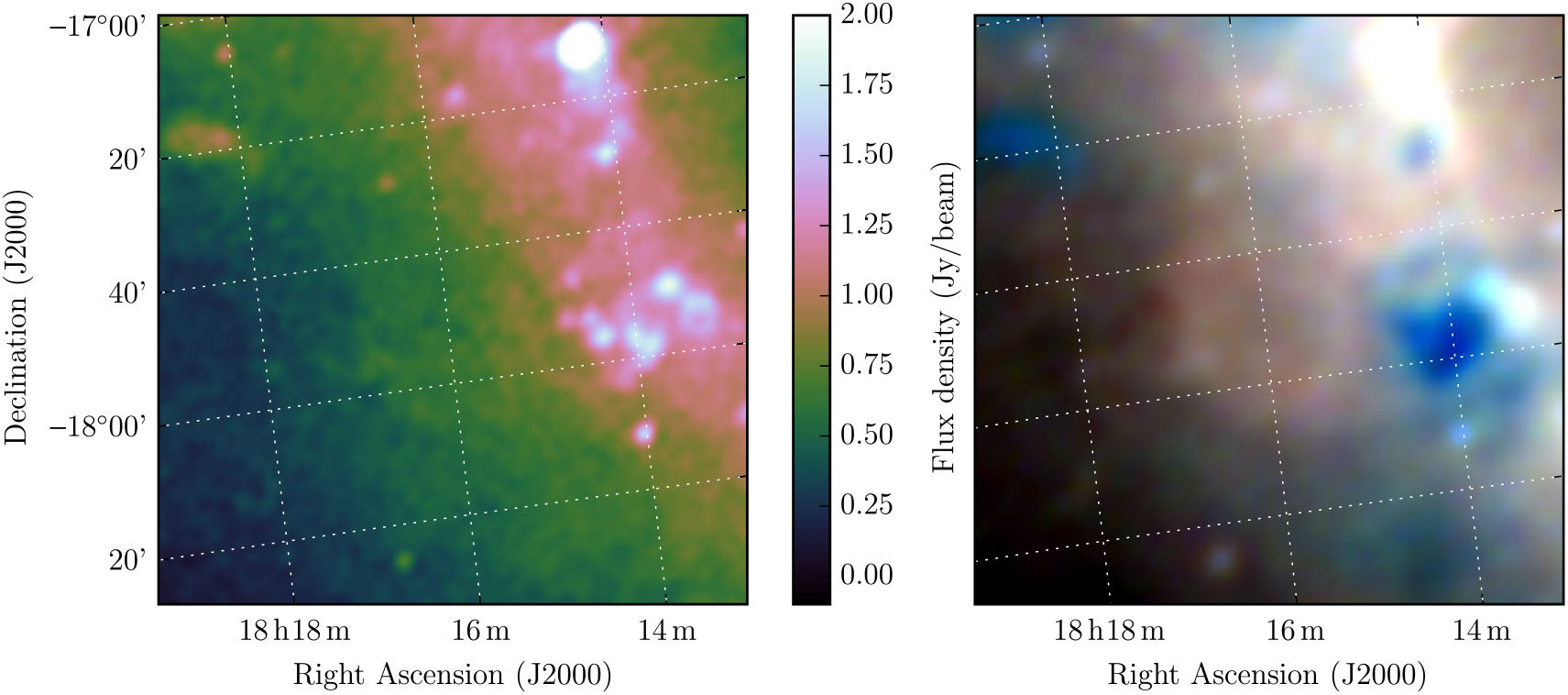
Brogan et al. (Reference Brogan, Gelfand, Gaensler, Kassim and Lazio2006) discovered 35 SNRs between 4.5° < l < 22.0° and |b| < 1.25°, using the VLA at 330 MHz. These remnants were ranked by the likelihood of being true SNRs, with Class III being the least likely. G15.51 – 0.15 fell into this class, despite meeting their three criteria for admission into the sample: a shell or partial-shell morphology, a negative spectral index, and no correlation with bright mid-IR μm emission. It was not further discussed, except to clarify that as Class III, it must be very faint, very confused, or does not exhibit a typical SNR morphology. It is just visible in the 11 cm Bonn survey of the Galactic Plane but at low significance and slightly confused with the other emission to the East. As one of a sample of 75 SNRs and 6 candidates, Hewitt & Yusef-Zadeh (Reference Hewitt and Yusef-Zadeh2009) searched G15.51 – 0.15 for maser emission, but did not make a detection, to a limit of ≈ 25 mJy at 0.53 km s−1 velocity resolution. No associated X-ray emission is seen in ROSAT, nor is there any significant 12 or 22 μm emission in WISE.
Our observations show that this source lies in a complex and confusing region, with two areas of low-frequency absorption (likely H ii regions) to the East and South, and the known SNR G15.4 + 0.1 to the West. Morphologically, it appears to be a complete and filled shell. Figure 18 shows the 200-MHz GLEAM image, and the RGB GLEAM cube at 72–103 MHz (R), 103–134 MHz (G), and 139–170 MHz (B), for G 15.51 – 0.15.
G15.51 – 0.15 as observed by GLEAM at 200 MHz (left) and at 72–103 MHz (R), 103–134 MHz (G), and 139–170 MHz (B) (right). The colour scales for the RGB cube are 3–7, 1.7–4, and 0.8–2 Jy beam–1, respectively. Black contours on the left panel show the NVSS data for the region, highlighting the compact source in the centre of the remnant. Levels are at 5, 35, 65, and 95 mJy beam–1. The local NVSS RMS noise level is 2 mJy beam–1.
There is also a potentially unrelated point source within the shell; running source-finding on the NVSS postage stamp for this region, we can find it has position RA = 18h19m23s Dec = +15d30m48s, size 1 × 1 arcmin with 1.4-GHz peak and integrated flux densities of 93 ± 3 mJy beam−1 and 163 ± 6 mJy, respectively. It is therefore unresolved by GLEAM; in the 170–231 MHz image it has a peak flux density of 1.5 Jy beam−1 and the local background (consisting of the shell of G15.5 – 0.2) is 1 Jy beam−1, so its flux density at 200 MHz is 0.5 Jy. Using the NVSS 1.4 GHz and GLEAM 200 MHz integrated flux densities, we calculate a spectral index of α = −0.58. The extrapolated flux density of this source is subtracted from each of the GLEAM measurements.
Excluding the nearby H ii regions and SNR G15.4 + 0.1 from the background calculation of G15.5 – 0.2, and subtracting the contaminating point source, yield a good spectral fit to the integrated flux density measurements, with S 200 MHz = 2.86 ± 0.29 Jy and α = −0.55 ± 0.03, typical for an SNR. This is very similar to the spectral index of the central radio source, perhaps indicating a common origin of the emission. Based on the spectral index, morphology, and lack of IR emission, we confirm G15.51 – 0.15 as an SNR.
3.1.17. G19.00 – 0.35
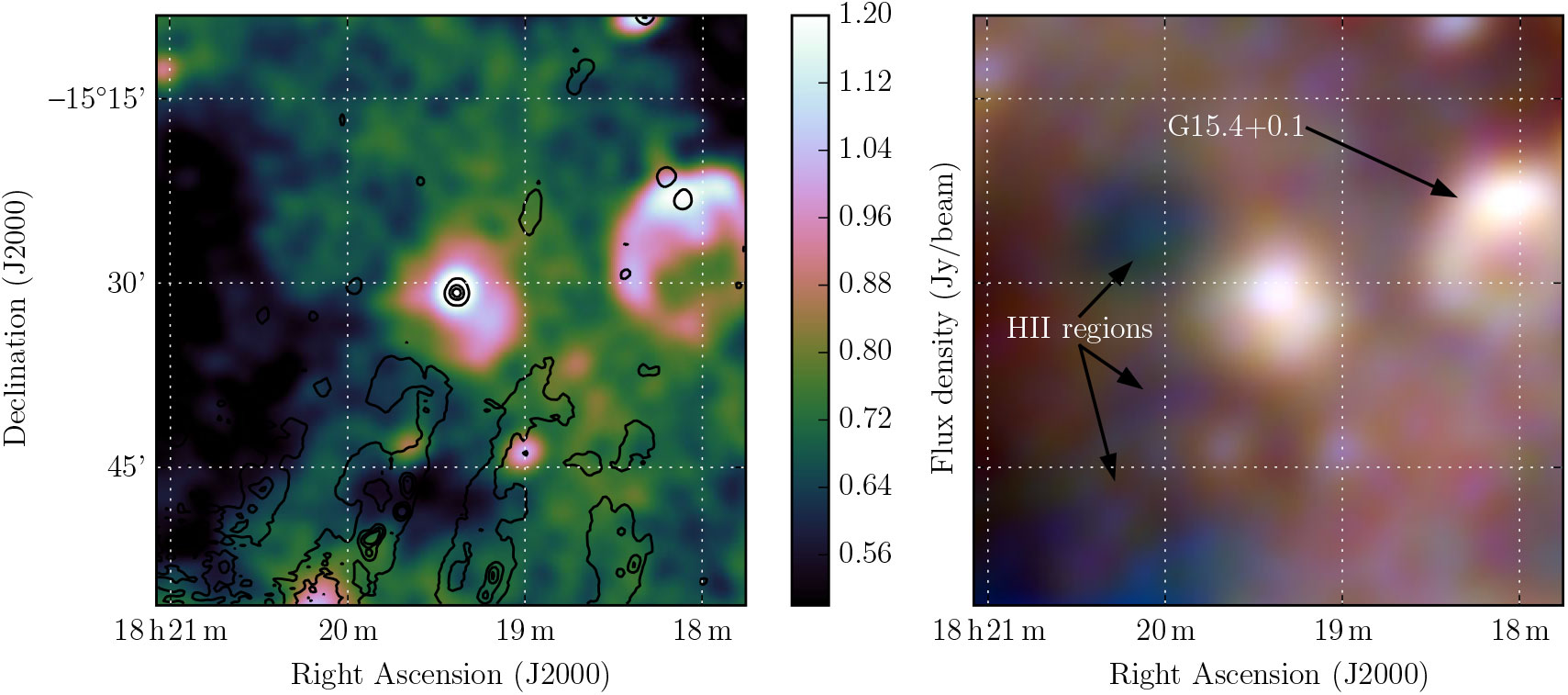
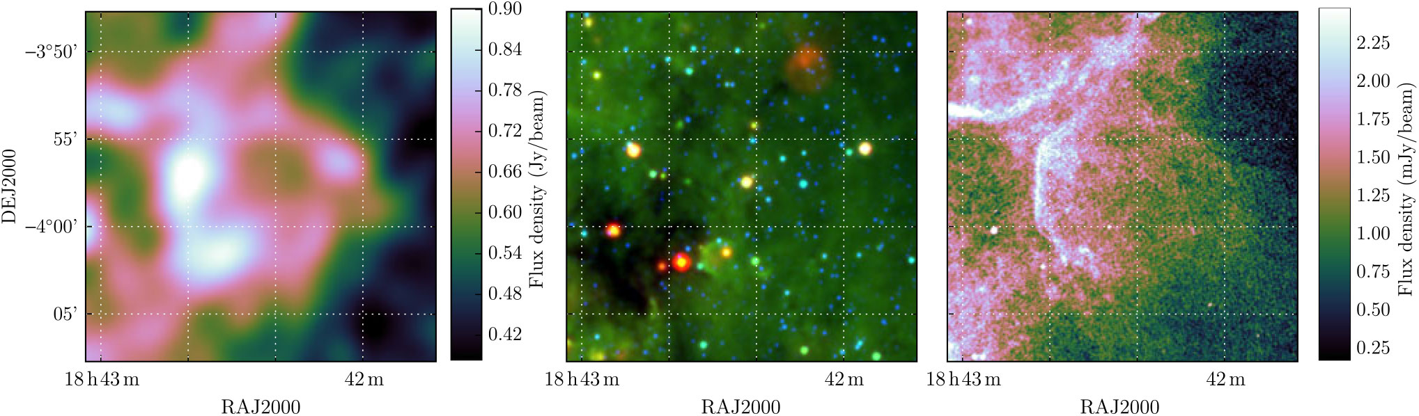
Another candidate proposed by Gosachinskii (Reference Gosachinskii1985) (see Section 3.1.14), G19.00 – 0.35 is described as having a 30’ diameter, with S 1.42GHz = 56 Jy and α = −0.48, therefore predicting S 200 MHz = 143 Jy. It is revealed as a complicated region of thermal and non-thermal emission by the GLEAM and WISE data, with S 200 MHz = 28 ± 2 Jy (see Figure 19). The dominant H ii region is visible in the WISE data (middle panel) as a bright loop of 12- and 22-μm emission, much brighter on the northwest side than the southeast; this is mirrored by the 200-MHz GLEAM data (right panel). In the GLEAM RGB cube (left panel), the free–free absorption of the low-frequency radio background over the whole loop becomes clear. Four or more non-thermal sources appear to be embedded in the complex. It is understandable that the Gaussian template fitting of Gosachinskii (Reference Gosachinskii1985) was unable to disentangle the complexity of this region. Now, however, we can state categorically that G19.00 – 0.35 is not an SNR.
G19.00 – 0.35 as observed by GLEAM (left) at 72–103 MHz (R), 103–134 MHz (G), and 139–170 MHz (B), by WISE (middle) at 22 μm (R), 12 μm (G), and 4.6 μm (B) and GLEAM at 200 MHz (right). The colour scales for the GLEAM RGB cube and wideband 200-MHz image are 2.8–9.0, 2.0–4.6, 1.0–2.4, and − 0.1–2.0 Jy beam−1, respectively. The candidate MAGPIS 18.6375 – 0.2917 is discussed in Section 3.2.
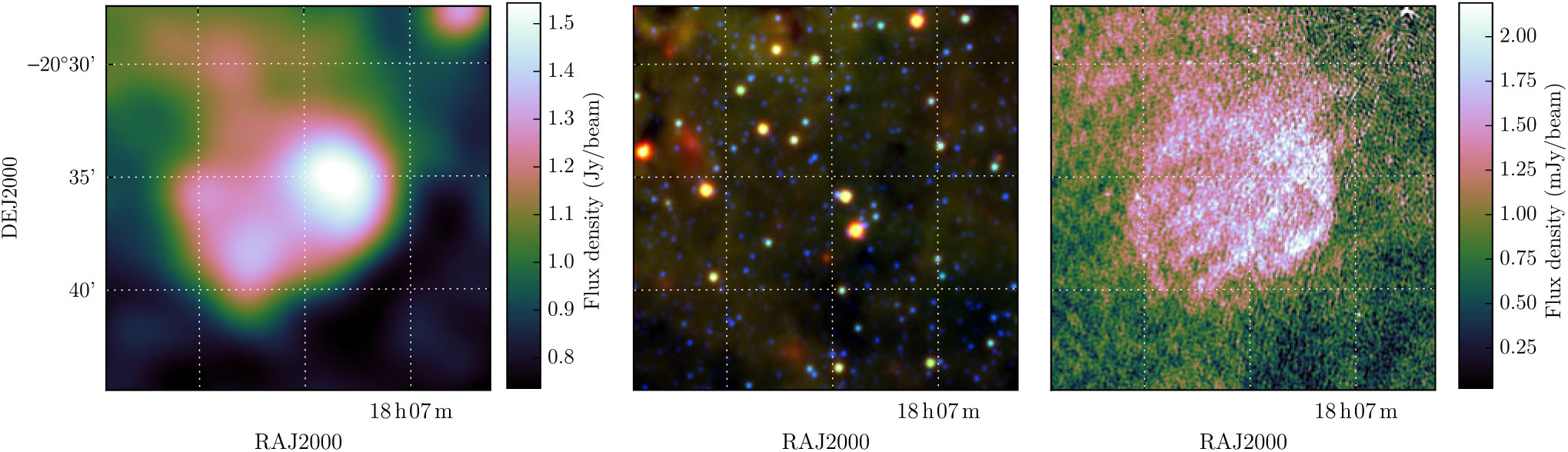
3.1.18. G35.40 – 1.80
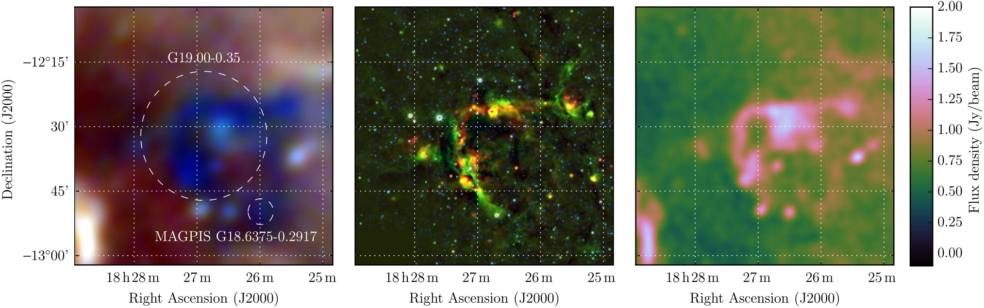
Also proposed by Gosachinskii (Reference Gosachinskii1985) as an SNR candidate, G35.40 – 1.80 was described as having 7’ extent, S 408 MHz = 7.9 ± 1.2 Jy, and α = −0.42, which would predict S 200 MHz = 10.7 ± 1.5 Jy. At the time of their observations, they did not consider this source to be part of the W48 H ii region complex, and specified W48 as a reference source to assist their flux calibration. Onello et al. (Reference Onello, Phillips, Benaglia, Goss and Terzian1994) classed all of the objects in this area as part of W48, with G35.40 – 1.80 labelled as W48C and W48D.Footnote q Using the VLA, they attempted to detect radio recombination lines (RRLs) toward W48A–E and were successful in all cases except for W48C. Despite this, the classification of W48C as an H ii region appears to have persisted in the literature.
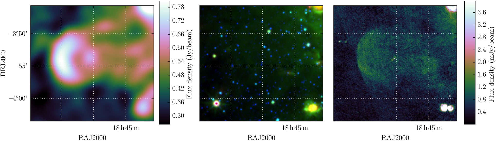
The compact source-finding of Hurley-Walker et al. (Reference Hurley-Walker2019c) detected G35.40 – 1.80 as two distinct components, GLEAM J190215 + 012219 (S 200 MHz = 0.97 ± 0.08, α = −0.82 ± 0.06) and GLEAM J190222 + 011904, for which S 200 MHz = 1.4 ± 0.1 Jy, and a distinct low-frequency turnover is observed. These objects are, respectively, the same as W48C and W48D, as classified by Onello et al. (Reference Onello, Phillips, Benaglia, Goss and Terzian1994). The non-thermal source, GLEAM J190215 + 012219, is also detected in VLSSr, TGSS-ADR1 and NVSS; Figure 20 shows a plot of the spectrum containing these and the GLEAM flux density measurements: combining them yields α = −0.85 ± 0.02 and S 200 MHz = 1.00 ± 0.09 Jy.
G35.40 – 1.80 and the W48 region, as observed by GLEAM at 72–103 MHz (R), 103–134 MHz (G), and 139–170 MHz (B) (left), WISE (middle), and NVSS (right). The colour scales for the GLEAM RGB cube are − 0.1–2.5 Jy beam−1. The five components ‘A’–‘E’ of W48 identified by Onello et al. (Reference Onello, Phillips, Benaglia, Goss and Terzian1994) are labelled on the right panel; C and D together make up the object G35.40 – 1.80 identified by Gosachinskii (Reference Gosachinskii1985) as an SNR candidate.
The thermal source, GLEAM J190222 + 011904, is resolved out by VLSSr and TGSS, and while it appears in NVSS images, is clearly not catalogued correctly by the automated source-finding. We use Polygon_Flux to measure S 1.4GHz = 1.73 ± 0.15 Jy from the NVSS image, but suspect that this is an underestimate of the true flux density due to the large angular extent (6’) of the source. Figure 21 shows a plot of this measurement, that of Onello et al. (Reference Onello, Phillips, Benaglia, Goss and Terzian1994), and the GLEAM flux density measurements.
The spectra of the two components of G35.40 – 1.80: the left panel shows the non-thermal source GLEAM J190215 + 012219 (W48C) and the right panel shows the H ii region GLEAM J190222 + 011904 (W48D). Black points indicate GLEAM measurements; red points indicate VLSSr (74 MHz), TGSS-ADR1 (150 MHz), and NVSS (1.4 GHz), while green squares show 1.362 GHz measurements made by Onello et al. (Reference Onello, Phillips, Benaglia, Goss and Terzian1994). In the left panel, the NVSS point is taken from the NVSS catalogue, while in the right panel, it has been measured using Polygon_Flux. Blue lines indicate least-squares power-law fits to the data; the left fit uses all plotted data points, while the right fit excludes the NVSS point and uses only the GLEAM data with ν > 150 MHz.
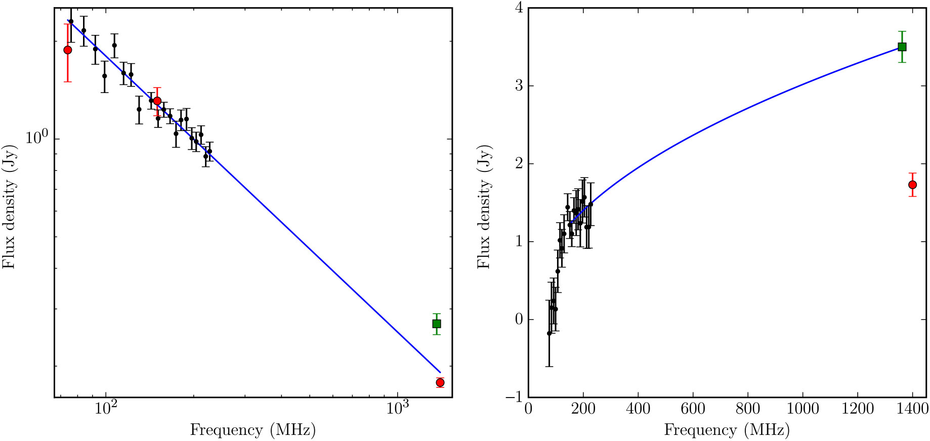
Based on the low-frequency free–free absorption, thermal radio spectrum, and the strong 12- and 22-μm emission seen in WISE, we confirm that W48D/GLEAM J190222 + 011904 is a H ii region. W48C / GLEAM J190215 + 012219 has no optical or IR counterpart; the nearest discrete source is an apparently unrelated galaxy at RA = 19h02m14.5s, Dec = +01d22m38s, 14 arcsec away. This unresolved source with no RRLs, and no optical or IR counterpart, α = −0.85, is a good candidate pulsar, or even a high-redshift radio galaxy. However, given α > − 1.3, it is still potentially an SNR, perhaps very young. Higher-resolution and/or pulsar timing observations will be necessary to reveal the nature of this source.
3.1.19. G36.00 + 0.00
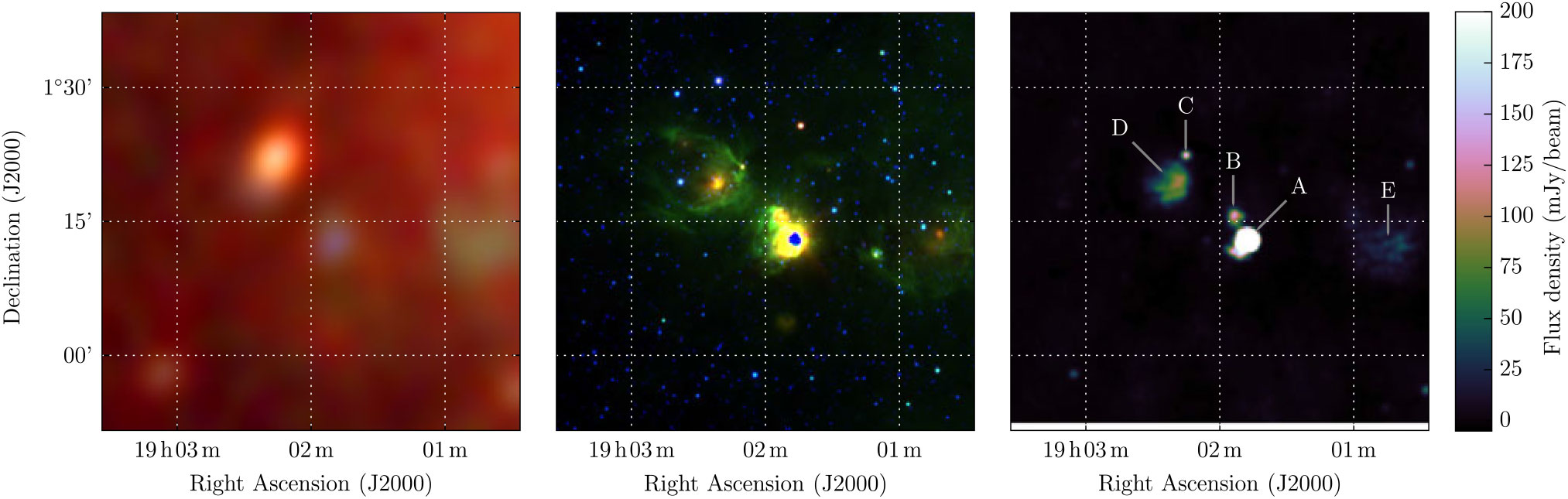
Ueno et al. (Reference Ueno, Yamauchi, Bamba, Yamaguchi, Koyama, Ebisawa, Meurs and Fabbiano2006) suggested G36.00 + 0.00 as a candidate SNR based on a diffuse X-ray excess of size ≈ 12 × 10 arcsec in the ASCA Galactic Plane Survey.
In the GLEAM images, there is no sign of diffuse emission on these scales, only an isolated point source. However, in TGSS-ADR1 and NVSS, this source is resolved into two individual sources, appearing at RA = 18h57m15.77s, Dec = +02d42m21.39s, and RA = 18h57m09.70s, Dec = +02d43m10.21s, and labelled A and B respectively in Figure 22. Neither appear in the NVSS catalogue, so we use Aegean to make measurements in the NVSS images, while we obtain TGSS flux densities directly from the ADR1 catalogue. Source A has S 150 MHz = 55 ± 10 mJy and S 1.4GHz = 24.8 ± 0.1 mJy, giving the source a spectral index of α = −0.36 ± 0.08. Source B has S 150 MHz = 540 ± 60 mJy and S 1.4GHz = 13.5 ± 0.1 mJy, giving the source a spectral index of α = −1.65 ± 0.04. For both sources combined, we measure S 200 MHz = 490 ± 90 mJy and α = −1.62 ± 0.15 across the GLEAM band, consistent with the TGSS-ADR1 and NVSS measurements.
G36.00 + 0.00 as observed by GLEAM (left) at 200 MHz, by NVSS (middle) at 1.4 GHz, and by Ueno et al. (Reference Ueno, Yamauchi, Bamba, Yamaguchi, Koyama, Ebisawa, Meurs and Fabbiano2006) with ASCA X-ray (2.0–7.0 keV) (right). Linear colour scales for GLEAM and NVSS are shown in the figure, while for ASCA, the scale is logarithmic and the numbers next to the scale bars correspond to the surface brightness in ×10−6 counts cm–2s−1arcmin–2. Dashed lines, white in the left and middle panel, and black in the right panel indicate Galactic coordinates. In the middle panel, the two compact radio sources discussed in the text are labelled A and B. In the right panel, the X-ray sources detected by Sugizaki et al. (Reference Sugizaki, Mitsuda, Kaneda, Matsuzaki, Yamauchi and Koyama2001) are designated with white crosses.
There is no obvious counterpart in WISE or DSS2 to either the diffuse X-ray source or the compact radio sources, and there are no known pulsars within the excess X-ray emission identified by Ueno et al. (Reference Ueno, Yamauchi, Bamba, Yamaguchi, Koyama, Ebisawa, Meurs and Fabbiano2006). We cannot confirm the status of G36.00 + 0.00 as an SNR, as we do not detect any diffuse component, but based on its steep spectrum and compact nature, we suggest Source B is a candidate pulsar.
3.2. MAGPIS candidates
Helfand et al. (Reference Helfand, Becker, White, Fallon and Tuttle2006) imaged 5° < l < 32° |b| < 0.8° with the VLA in multiple configurations at 1.4 GHz, to a noise level of ≈2 mJy beam−1, to create the MAGPIS. They compared this data to 330 MHz VLA data and the 21 μm MSX Point Source Catalog version 2.3 ‘MSX6C’ dataset (Egan et al. Reference Egan, Price and Kraemer2003), in order to detect new compact Galactic objects and distinguish H ii regions from SNR. They presented 49 ‘high-probability’ candidate SNR, requiring the object to be undetected in MSX6C, brighter at 330 MHz than at 1.4 GHz, and have a shell-like or pulsar wind nebula (PWNe)-like morphology. Due to the high resolution of the VLA survey, these are all relatively compact objects, with diameters ≤14' and typically ≈3′, and are therefore usually unresolved by GLEAM.
The MSX6C dataset and 330 MHz VLA data appear not to have been sensitive enough to completely discriminate SNR from H ii regions. The WISE data is ≈300× more sensitive than the MSX data and reveals that 31 of these candidate SNRs are associated with strong 12- and sometimes 22-μm emission, which is morphologically similar to the radio emission. Three are coincident with known H ii regions observed in the canonical survey of Lockman (Reference Lockman1989). Johanson and Kerton (Reference Johanson and Kerton2009) measured the H i absorption spectra toward the 41 candidates to attempt to measure their distances, and reclassified a further nine as H ii regions based on strong RRL emission, 8-μm GLIMPSE, or 24-μm MIPSGAL emission. Anderson et al. (Reference Anderson2017) reclassified a further eight MAGPIS SNR candidates as known H ii regions, based on their IR emission in WISE, as well as another MAGPIS candidate as a known planetary nebula (PN). Ten SNRs were accepted to the catalogue of Green (Reference Green2014). Table 2 summarises the MAGPIS candidates, extending Table 4 of Helfand et al. (Reference Helfand, Becker, White, Fallon and Tuttle2006) to include the GLEAM measurements and morphological classifications, where possible. The total number of candidates previously confirmed as SNRs is 10, reclassified as H ii regions is 20, with one further object reclassified as a PN.
MAGPIS SNR candidates; the first four columns are taken from Table 4 of Helfand et al. (Reference Helfand, Becker, White, Fallon and Tuttle2006); the next four columns are calculated in Section 3.2. ‘Class’ is determined from the literature where possible, or this work if the GLEAM spectrum and/or morphology are clear: ‘–’ indicates that the GLEAM data do not improve our understanding of this candidate.
Of the 10 SNR added to the catalogue of Green (Reference Green2014), we detect and measure eight, including spectral indices for three, which are uniformly non-thermal. MAGPIS 29.366700 + 0.100000 is noted as a potential PWNe by Helfand et al. (Reference Helfand, Becker, White, Fallon and Tuttle2006); the GLEAM spectrum of α = −0.09 ± 0.14 is consistent with a PWNe interpretation. Morphologically in the MAGPIS data, it resembles a wide-angle tail radio galaxy, but there is no obvious host visible in WISE or DSS2. There is also a somewhat filled shell visible in both MAGPIS and GLEAM. We therefore tentatively confirm this SNR as a composite SNR with central emission and a surrounding shell.
Of the 20 candidates already reclassified as H ii regions, we observe eight as regions absorbing low frequencies in GLEAM, further increasing the likelihood that they are H ii regions. We have noted their rising spectra in Table 2 (α > 0), but do not attempt to fit power-law spectral indices as these do not sufficiently describe the spectra. The upcoming publication Su et al. (in prep.) will publish the GLEAM spectra for these objects, as well as all other detected H ii regions in the data release of Hurley-Walker et al. (Reference Hurley-Walker2019c).
Of the 18 unconfirmed and not-previously reclassified objects, we detect seven in GLEAM. MAGPIS 9.683300 – 0.066700, MAGPIS 28.375000 + 0.202800, and MAGPIS 28.7667 – 0.4250 have non-thermal spectra and shell-like morphology and are easily confirmed as SNRs (Figures 23, 24, 25, respectively). MAGPIS 18.6375 – 0.2917 appears in absorption and overlaps with the candidate G 19.00 – 0.35 (Section 3.1.17), which we reclassify as a H ii region; its location is marked on Figure 19. Similarly, MAGPIS 20.4667 + 0.1500 also has a thermal spectrum with absorption at low frequencies (Figure A34), so we class it as a H ii region. The spectrum of these two candidates is indicated with α > 0 in Table 2.
MAGPIS 9.683300 – 0.066700 as observed by GLEAM at 200 MHz (left), WISE at 22 μm (R), 12 μm (G), and 4.6 μm (B), and by MAGPIS at 1.4 GHz (right).
MAGPIS 28.375000 + 0.202800 as observed by GLEAM at 200 MHz (left), WISE at 22 μm (R), 12 μm (G), and 4.6 μm (B), and by MAGPIS at 1.4 GHz (right).
MAGPIS 28.7667 – 0.4250 as observed by GLEAM at 200 MHz (left), WISE at 22 μm (R), 12 μm (G), and 4.6 μm (B), and by MAGPIS at 1.4 GHz (right).
MAGPIS 27.133300 + 0.033300 appears to be a single lone arc of emission, reminiscent of part of an SNR shell (Figure 26). There is a H ii region to the south which could be confused as a counterpart arc were it not for the WISE data, which shows strong 12- and 22-μm emission. There is another non-thermal region of emission to the south-west which has a similar filamentary morphology in MAGPIS, and is likely the other half of the shell. Unfortunately the region is strongly confused in GLEAM, with many nearby H ii regions, making it difficult to extract reliable flux density measurements. Table 2 therefore has only a 200-MHz measurement for this source, and only for the single arc as seen in MAGPIS.
MAGPIS 18.758300 – 0.073600 is small and located in a confused region, so while we may make a flux density measurement, it is unresolved by GLEAM. It is noted as a potential PWNe by Helfand et al. (Reference Helfand, Becker, White, Fallon and Tuttle2006). Due to its small size (1′.6), we can use NVSS to measure its 1.4-GHz flux density as 22.8 ± 1.5 mJy, implying a spectral index between 200 and 1400 MHz of − 1.8, which is highly incompatible with a PWNe interpretation, which we have indicated in Table 2.
MAGPIS 27.133300 + 0.033300 as observed by GLEAM at 200 MHz (left), WISE at 22 μm (R), 12 μm (G), and 4.6 μm (B), and by MAGPIS at 1.4 GHz (right).
It would be ideal to use the MAGPIS 1.4-GHz integrated flux density measurement to constrain the spectra of all 13 SNR candidates measurable in GLEAM, but Helfand et al. (Reference Helfand, Becker, White, Fallon and Tuttle2006) note that their flux density scale has a large amount of uncertainty, and that integrated flux densities are unreliable and often overestimated by large and varying factors. Our measurements confirm this, finding that for the five sources where we are able to derive full spectra, the resulting 1.4-GHz flux density prediction is of order 6–25 % of the values obtained by MAGPIS.
4. Discussion
Of the 101 non-MAGPIS candidates proposed in the region, 82 are undetectable in these data. Given the range of different origins of these candidates, it is difficult to draw any particular conclusions about how one might improve the detection rate. Certainly, higher sensitivity by increasing the integration time may be useful for the larger and fainter objects. In all, 51 have diameters ≤5 arcmin, so arcminute or better resolution may help reveal the nature of these sources. The upcoming GLEAM-eXtended (GLEAM-X; Hurley-Walker et al., in prep.) survey using the upgraded MWA will have up to 10× the sensitivity of GLEAM, and double the resolution. This should be a valuable resource for determining the nature of many of the remaining candidates.
Low frequencies appear to offer a decided advantage in finding new SNRs over high frequencies, where both thermal and non-thermal emission have similar contributions to the Galactic brightness. Of the 49 MAGPIS candidates, 30 are in fact H ii regions, while Hurley-Walker et al. (Reference Hurley-Walker2019b) show 27 new SNRs detected at low frequencies with no IR counterparts, many with pulsar associations, and Johnston-Hollitt et al. (in prep.) find similar results over the region 240° < l < 345°.
The wide bandwidth of the MWA has been particularly useful in discriminating between types of emission, due to the distinct absorption signature of the H ii regions. However, wide bandwidths at higher frequencies, such as those available to the Australian Square Kilometer Array Pathfinder (ASKAP; Hotan et al. Reference Hotan2014), should also allow useful discrimination between thermal and non-thermal emission. Indeed, the combination of upcoming radio surveys in the Southern Hemisphere from both the MWA and ASKAP will offer powerful insights into Galactic astrophysics and should result in many more SNR detections. Flux density calibration across multiple epochs and instruments is key: the poor flux calibration of MAGPIS appears to have hindered their ability to produce reliable spectra, contaminating their candidate sample.
As the population of known Galactic SNRs grows, more SNR will be found in line-of-sight overlap, and require careful analysis to separate the different objects. There are likely a further ≈700 SNRs yet to be discovered, and many will naturally be overlapping. High resolution and high surface brightness sensitivity will become exponentially more important as the counts of SNRs increase.
5. Conclusions
We examined the latest data release from the GLEAM survey covering 345° < l < 60° and 180° < l < 240°, using these data and that of the WISE to follow up proposed candidate SNRs from other sources. Of the 101 candidates proposed in the region, we are able to definitively confirm ten as SNRs, tentatively confirm two as SNRs, and reclassify five as H ii regions. A further two are detectable in our images but difficult to classify; the remaining 82 are undetectable in these data. We also investigated the 18 unclassified MAGPIS candidate SNRs, newly confirming three as SNRs, reclassifying two as H ii regions, and exploring the unusual spectra and morphology of two others.
Acknowledgements
We thank the anonymous referee for their comments, which improved the paper. This scientific work makes use of the Murchison Radio-astronomy Observatory, operated by CSIRO. We acknowledge the Wajarri Yamatji people as the traditional owners of the Observatory site. Support for the operation of the MWA is provided by the Australian Government (NCRIS), under a contract to Curtin University administered by Astronomy Australia Limited. We acknowledge the Pawsey Supercomputing Centre which is supported by the Western Australian and Australian Governments. We acknowledge the work and support of the developers of the following python packages: Astropy The Astropy Collaboration et al. (2013), Numpy (van der Walt et al. Reference van der Walt, Colbert and Varoquaux2011), and Scipy (Jones et al. Reference Jones, Oliphant and Peterson2001). We also made extensive use of the visualisation and analysis packages DS9Footnote r and Topcat (Taylor Reference Taylor, Shopbell, Britton and Ebert2005). This publication makes use of data products from the Wide-field Infrared Survey Explorer, which is a joint project of the University of California, Los Angeles, and the Jet Propulsion Laboratory/California Institute of Technology, funded by the National Aeronautics and Space Administration.
Appendix A. List of candidate SNRs searched
SNR candidates searched for in this work, ordered first by detection method, second by date detected, and third by l.
Appendix B. Regions used to determine SNR flux densities
These plots follow the format of Figure 1, indicating where the polygons were drawn in Polygon_Flux to measure SNRs. The top two panels of each figure show the GLEAM 170–231 MHz images; the lower two panels show the RGB cube formed from the 72–103 MHz (R), 103–134 MHz (G), and 139–170 MHz (B) images. As described in Section 2.4, the annotations on the right two panels consist of: white polygons to indicate the area to be integrated in order to measure the SNR flux density; blue dashed lines to indicate regions excluded from any background measurement; the light shaded area to show the region that is used to measure the background, which is then subtracted from the final flux density measurement. Figures proceed in order of Galactic longitude, first for the outer-Galactic ‘oG’ region (180° < l < 240°), and then the inner-Galactic ‘iG’ region (345° < l < 60°). SNRs for which no GLEAM spectra was extracted are excluded from this list.
Polygons drawn over GLEAM images to measure source and background flux densities for G345.1 – 0.2.
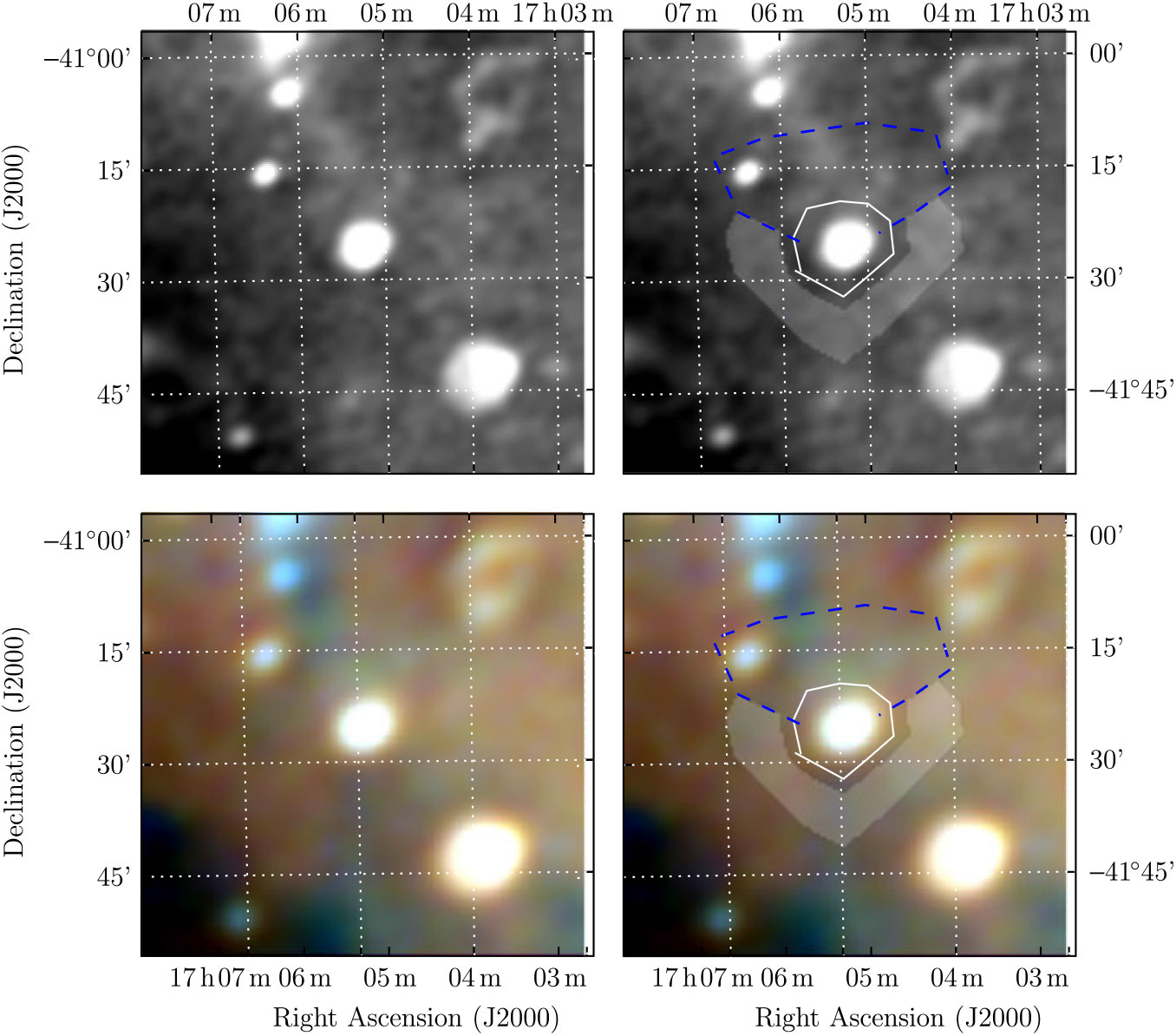
Appendix C. Spectra
The spectra of the measured SNR using the backgrounding and flux summing technique are described in Section 2.4. The left panels show flux density against frequency with linear axes while the right panels show the same data in log. (It is useful to include both when analysing the data as a log plot does not render negative data points, which occur for faint SNRs). The black points show the (background-subtracted) SNR flux density measurements, the red points show the measured background, and the blue curve shows a linear fit to the log–log data (i.e. S ν ∝ ν α ). The fitted value of α is shown at the top right of each plot.
Polygons drawn over GLEAM images to measure source and background flux densities for G345.1 + 0.2.
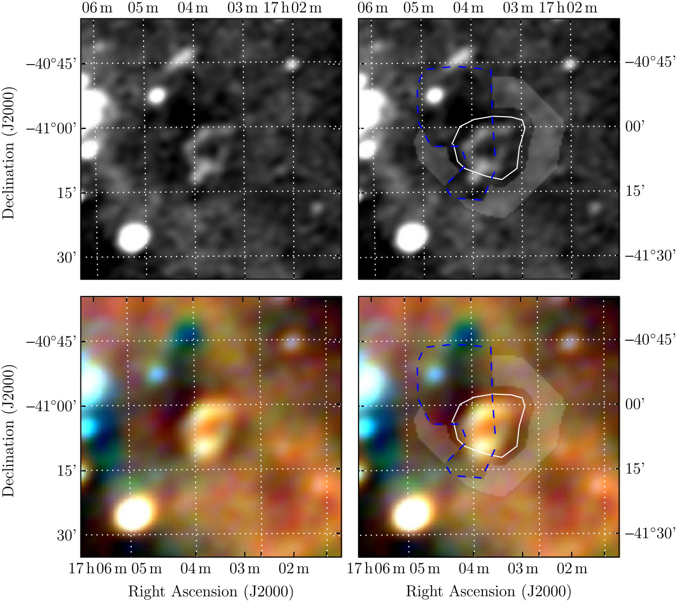
Polygons drawn over GLEAM images to measure source and background flux densities for G348.8 + 1.1.
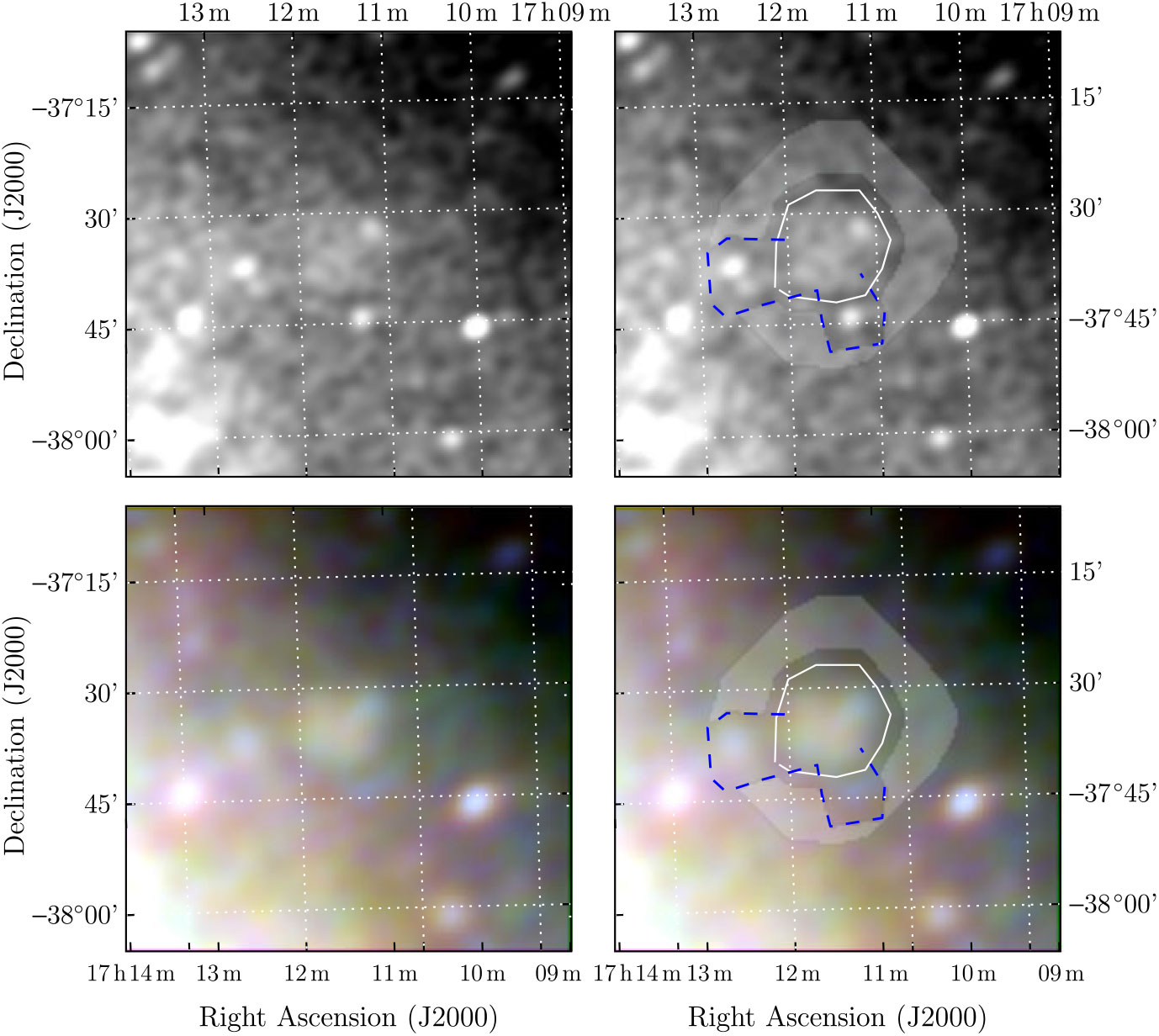
Polygons drawn over GLEAM images to measure source and background flux densities for G352.2 –0.1.
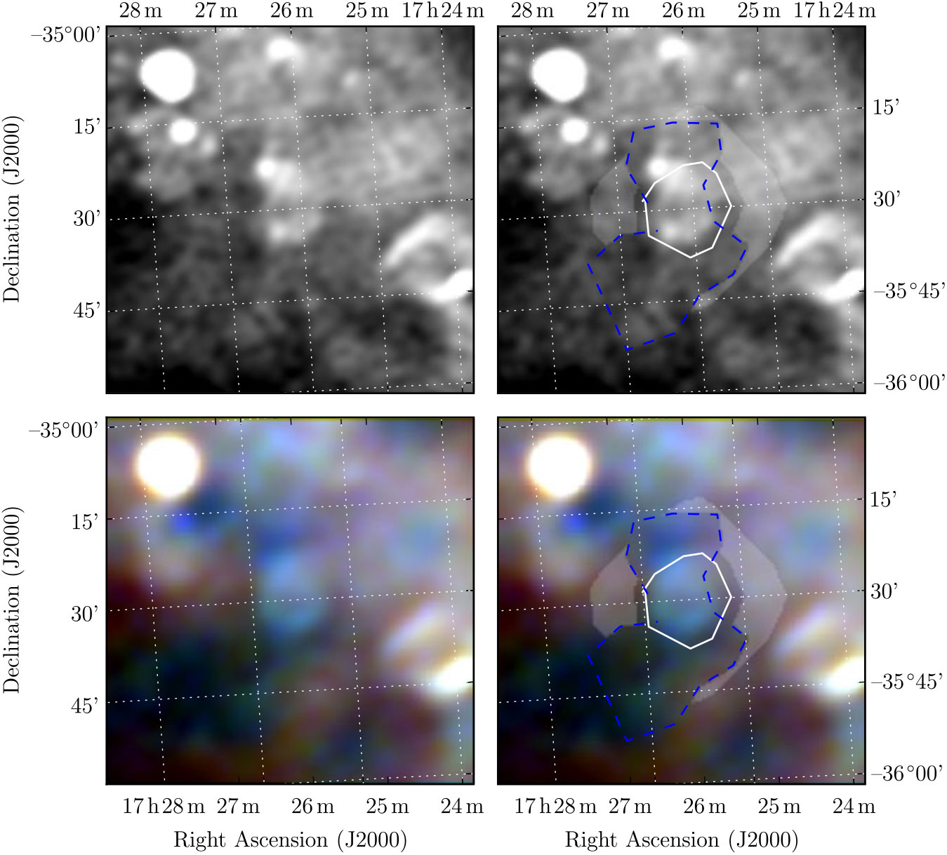
Polygons drawn over GLEAM images to measure source and background flux densities for G353.3–1.1.
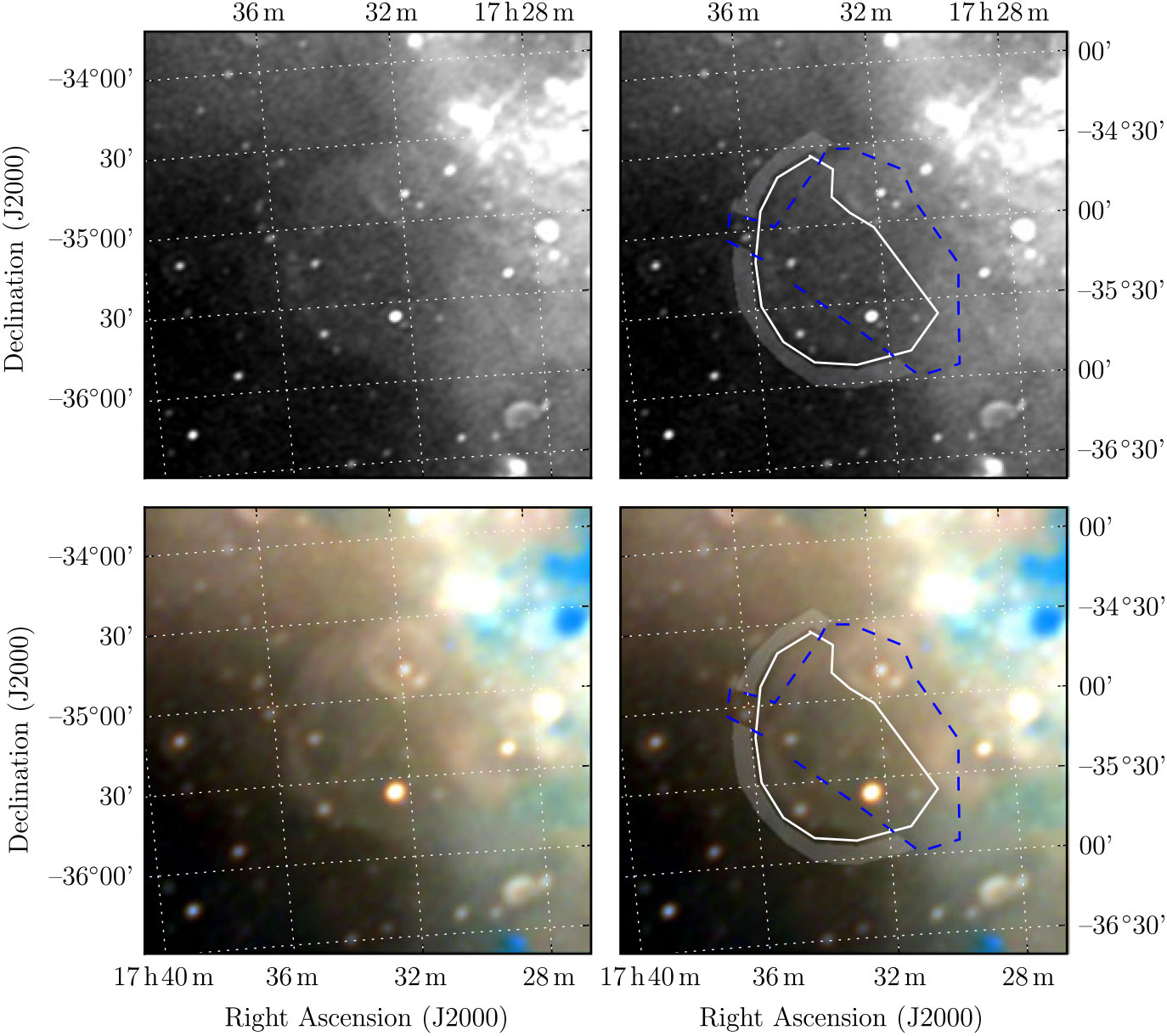
Polygons drawn over GLEAM images to measure source and background flux densities for G354.46 + 0.07.
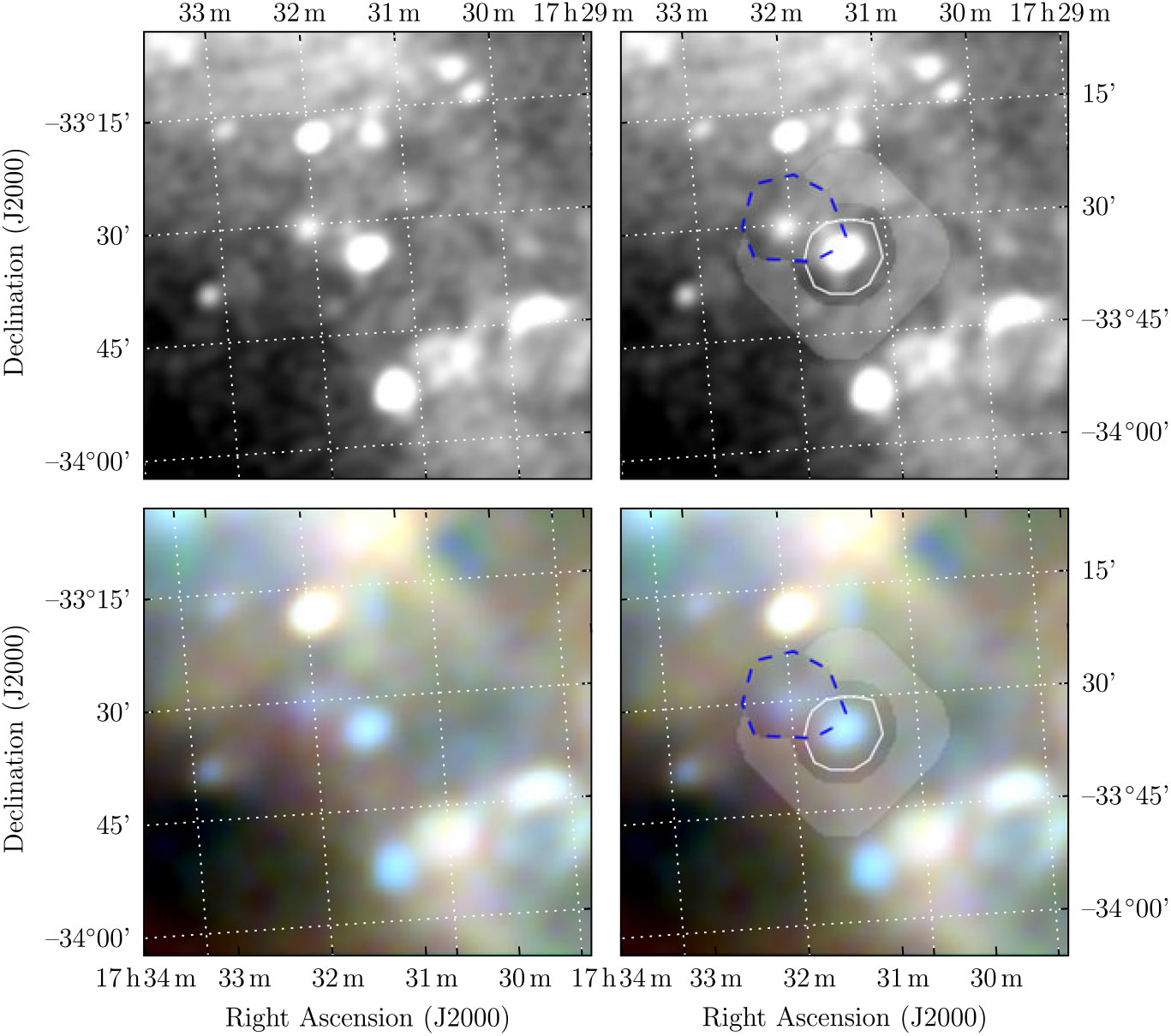
Polygons drawn over GLEAM images to measure source and background flux densities for G356.6 + 00.1.
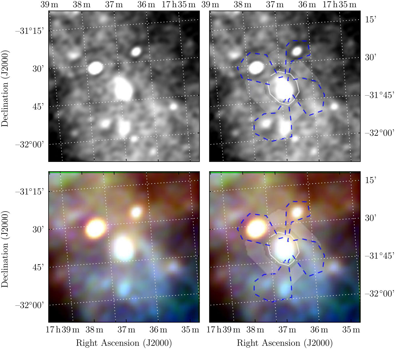
Polygons drawn over GLEAM images to measure source and background flux densities for G359.2 –01.1.
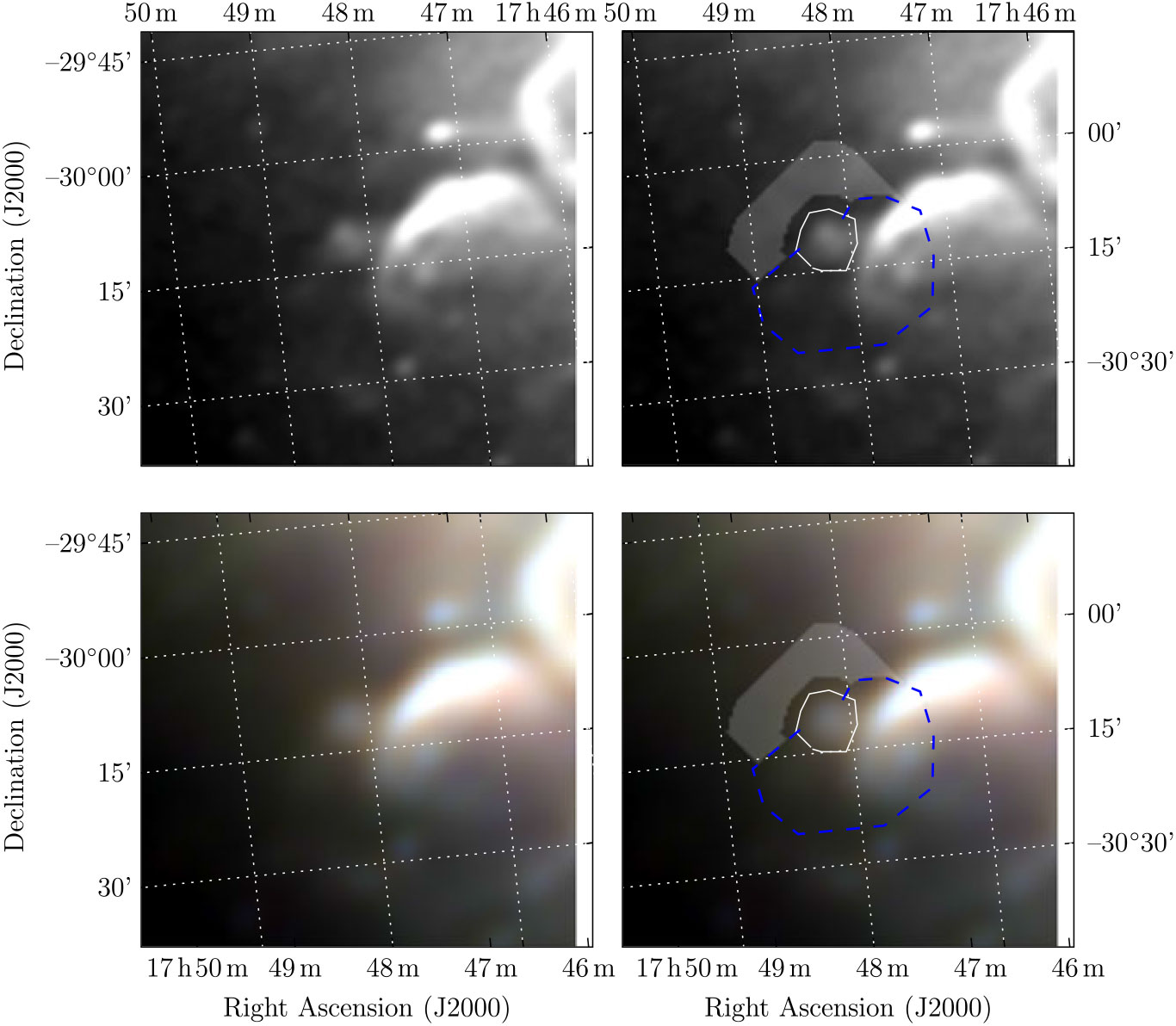
Polygons drawn over GLEAM images to measure source and background flux densities for G3.1–0.7.
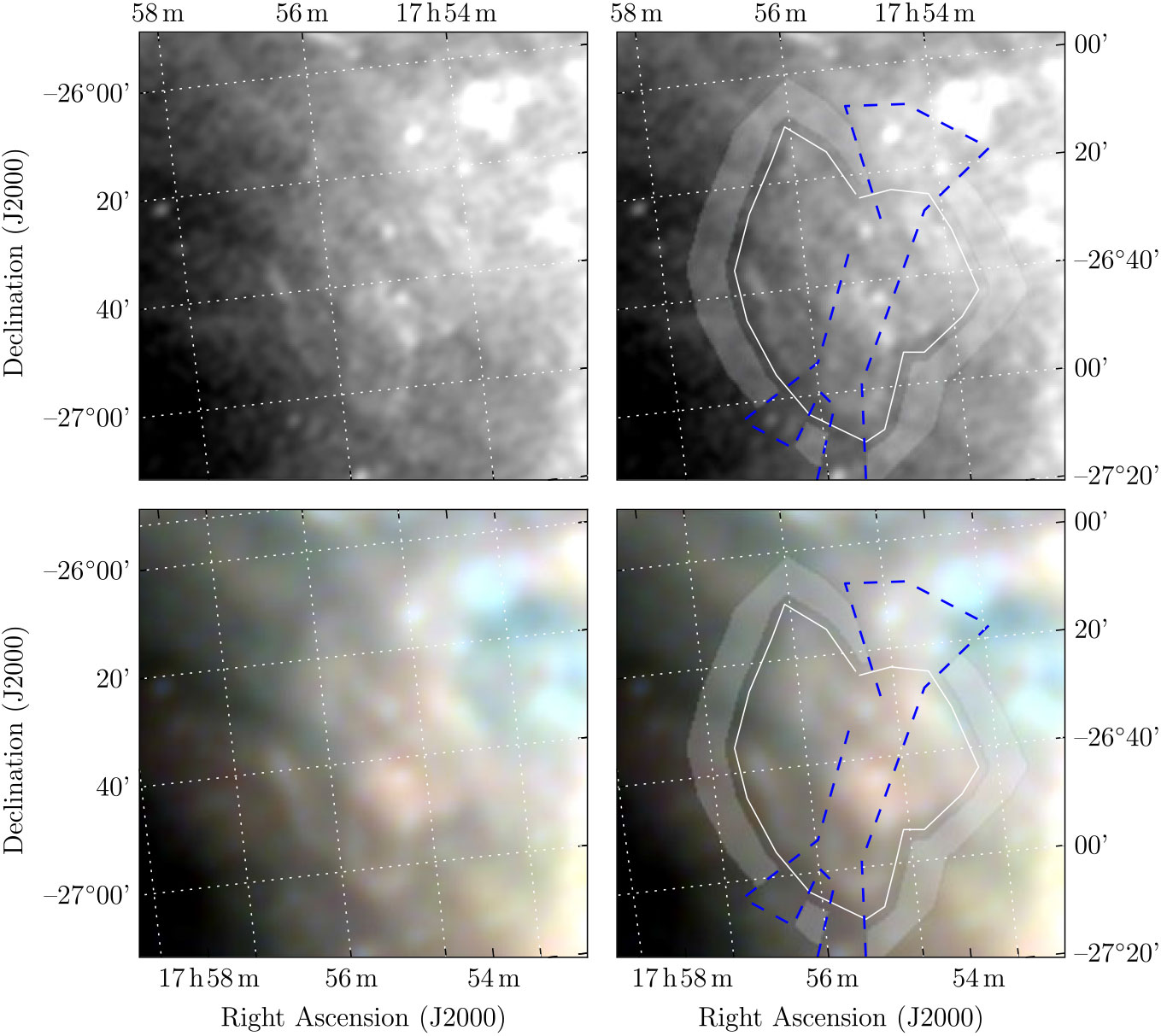
Polygons drawn over GLEAM images to measure source and background flux densities for G7.5–1.7.
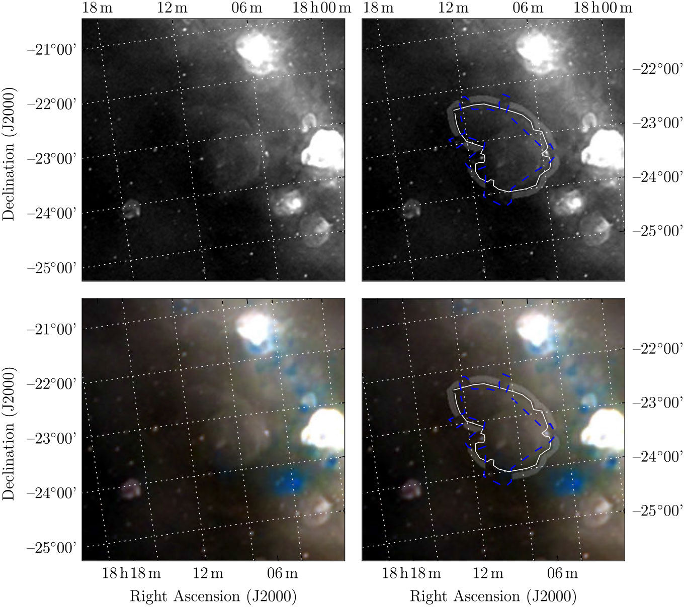
Polygons drawn over GLEAM images to measure source and background flux densities for G13.1–0.5.
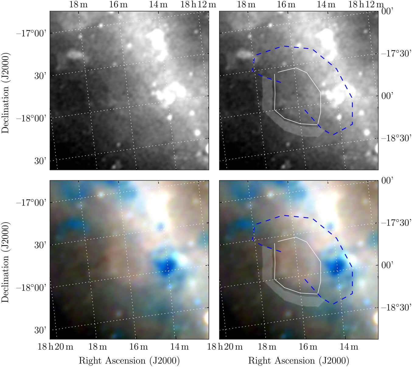
Polygons drawn over GLEAM images to measure source and background flux densities for G15.51–0.15.
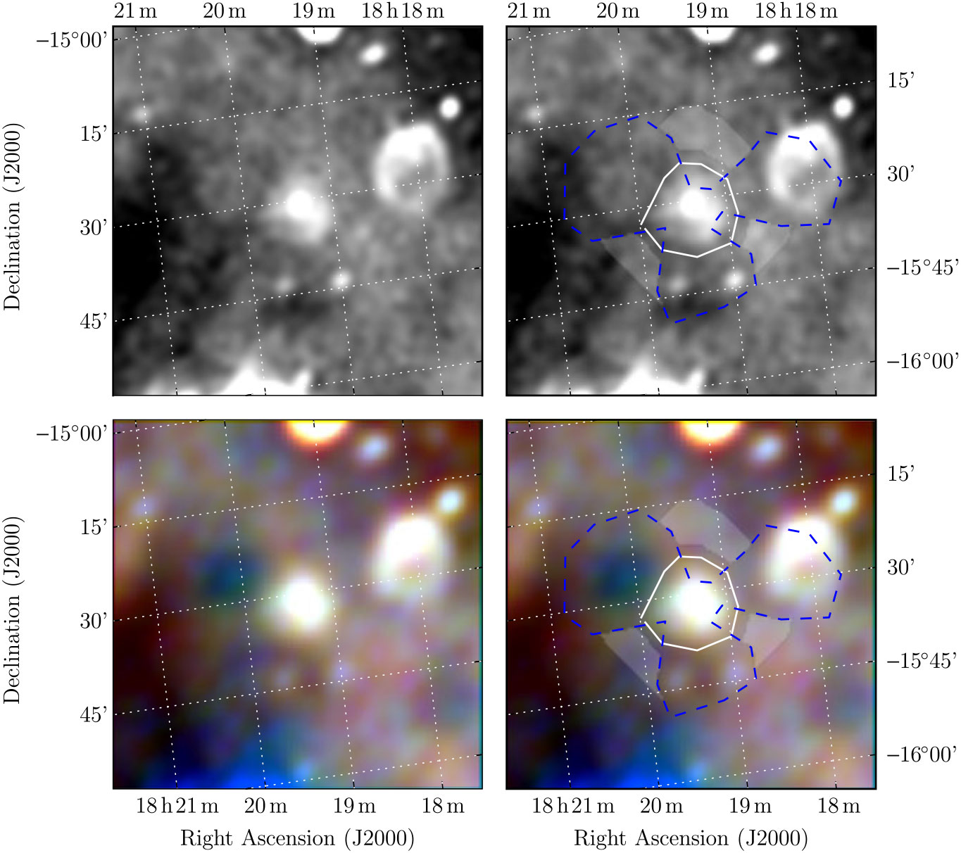
Polygons drawn over GLEAM images to measure source and background flux densities for MAGPIS 9.6833 − 0.0667.
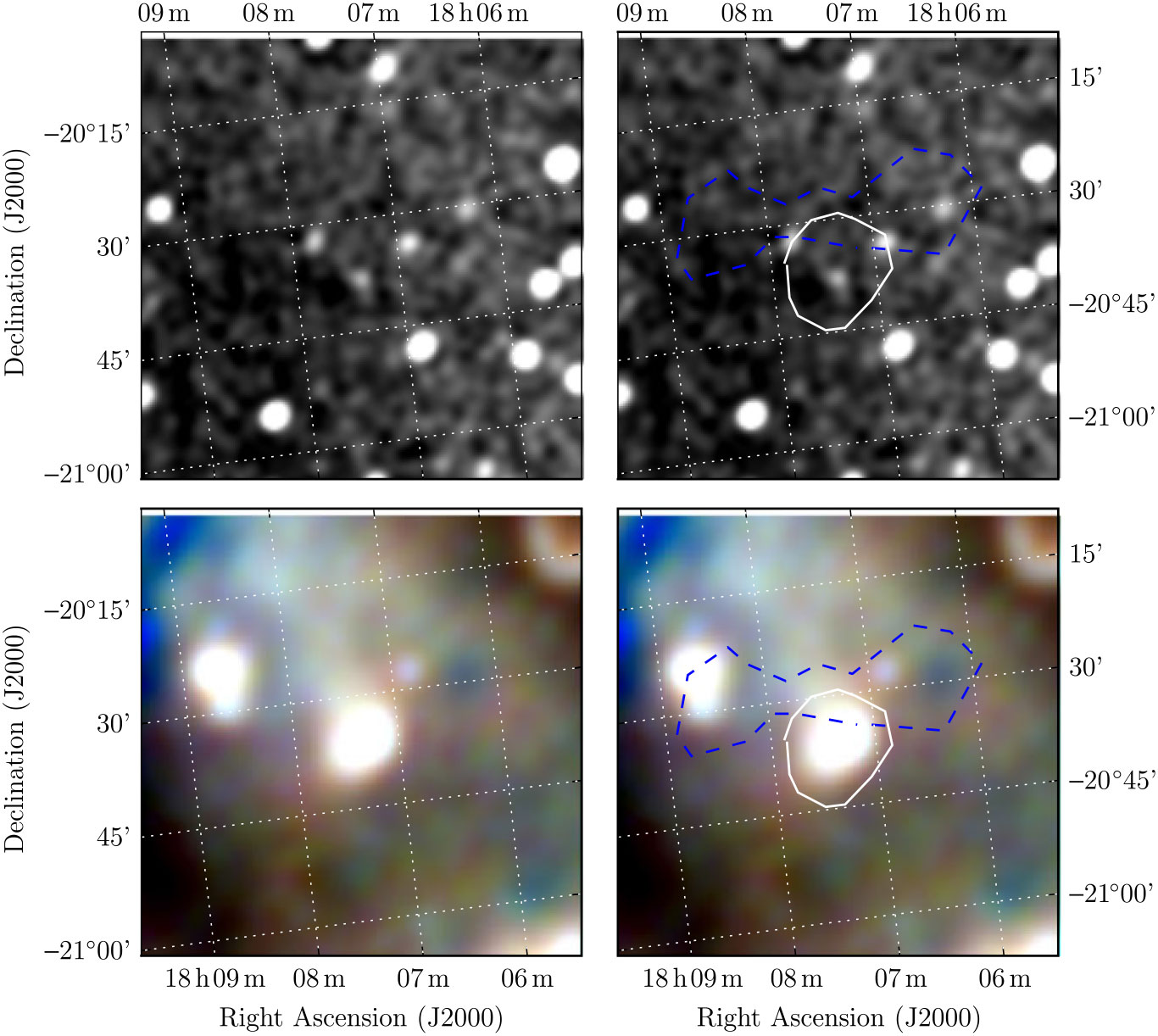
Polygons drawn over GLEAM images to measure source and background flux densities for MAGPIS 28.3750 + 0.2028.
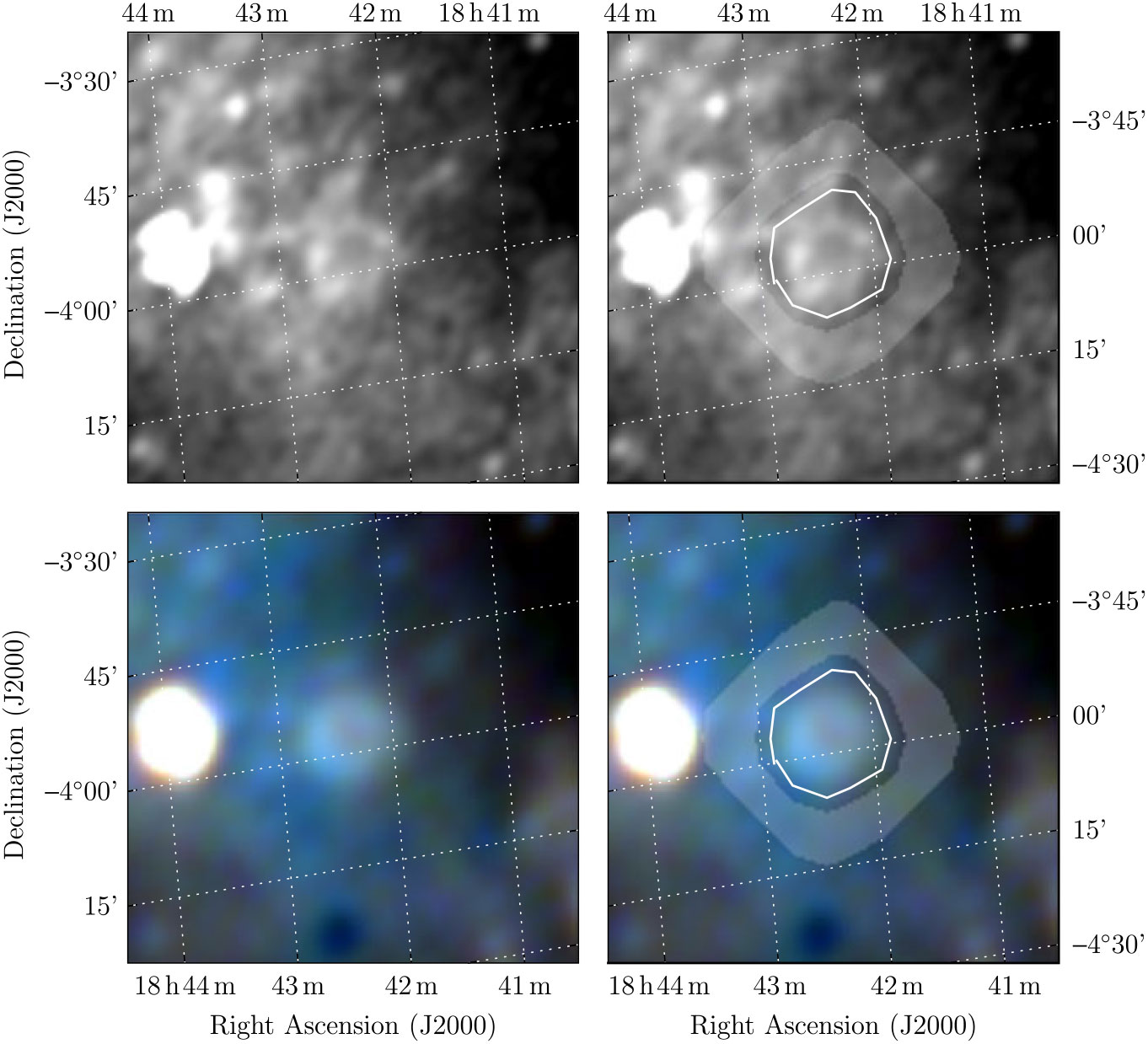
Polygons drawn over GLEAM images to measure source and background flux densities for MAGPIS 28.7667 − 0.4250.
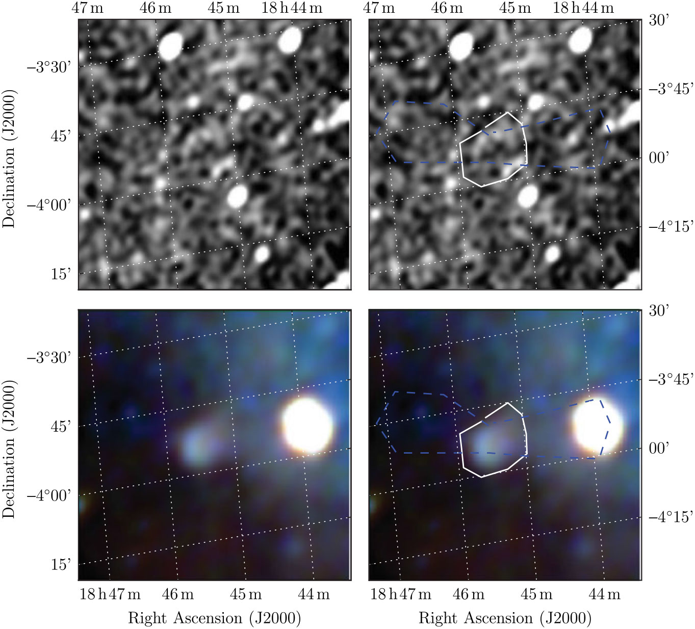
Polygons drawn over GLEAM images to measure source and background flux densities for MAGPIS 27.1333 + 0.0333.
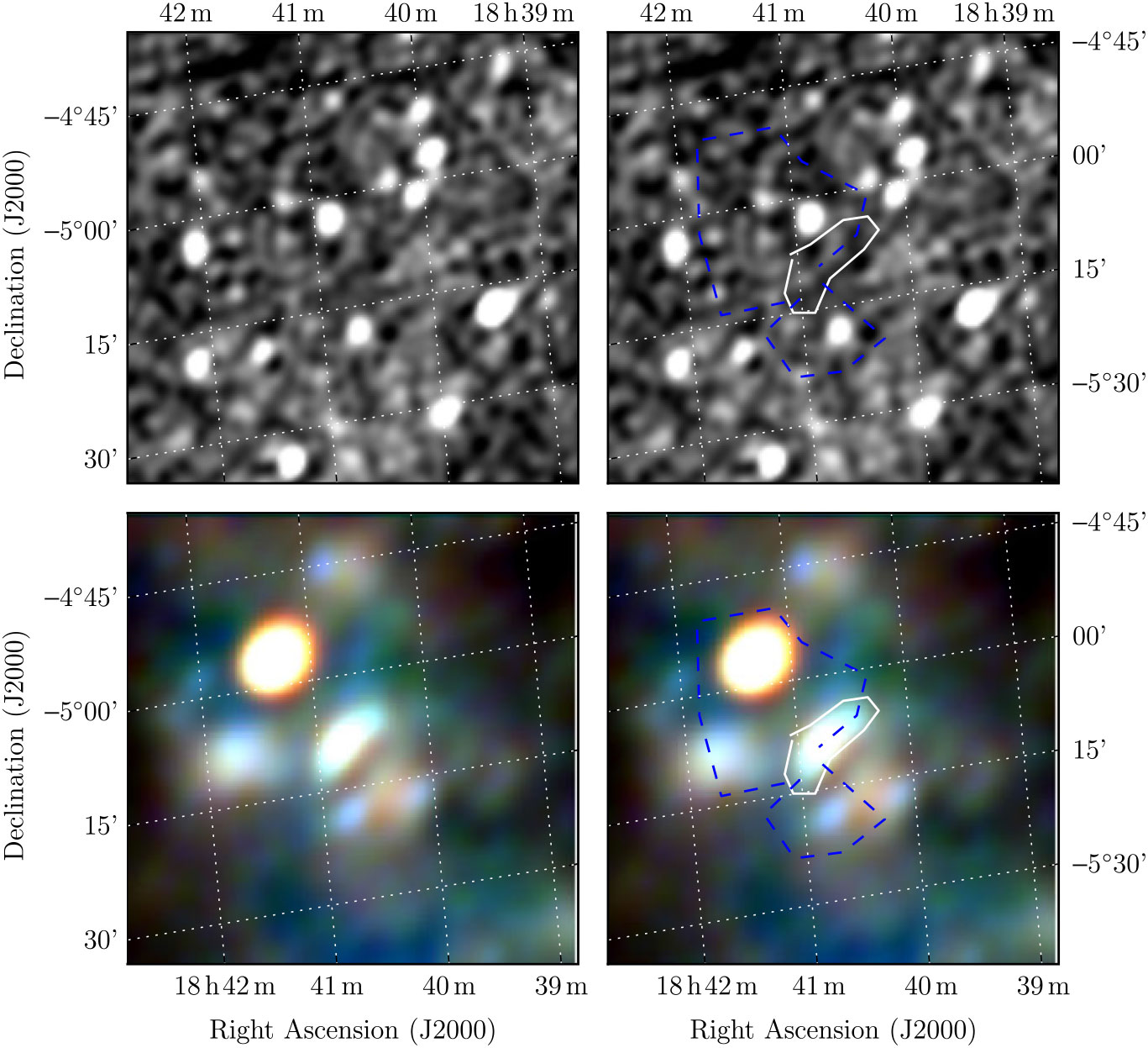
Polygons drawn over GLEAM images to measure source and background flux densities for MAGPIS 20.4667 + 0.1500.
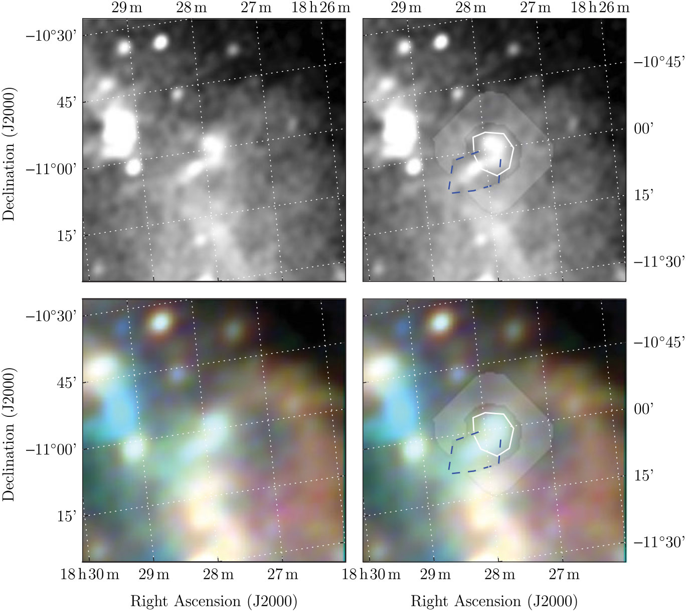
Spectral fitting over the GLEAM band for G345.1–0.2.

Spectral fitting over the GLEAM band for G345.1 + 0.2.
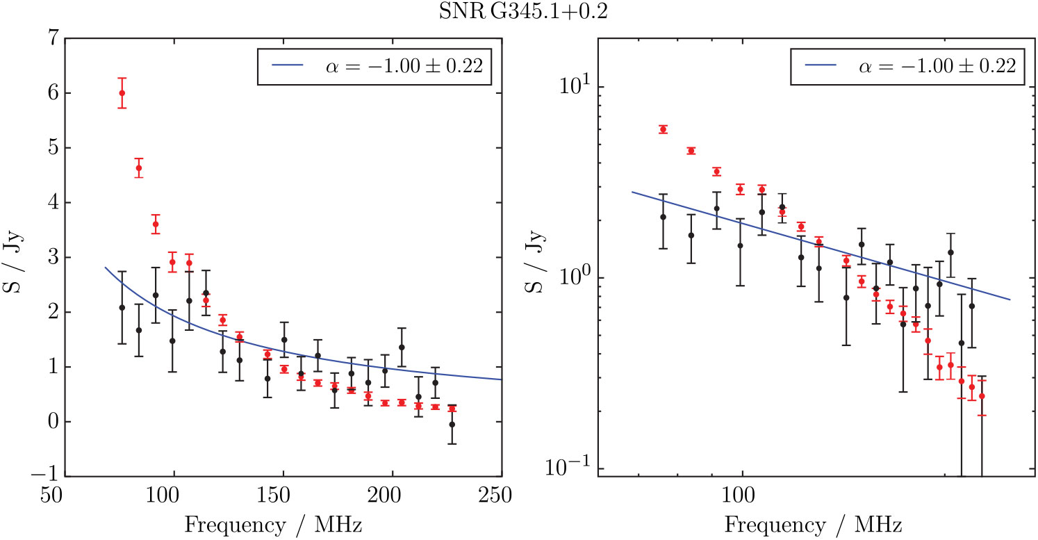
Spectral fitting over the GLEAM band for G348.8 + 1.1.
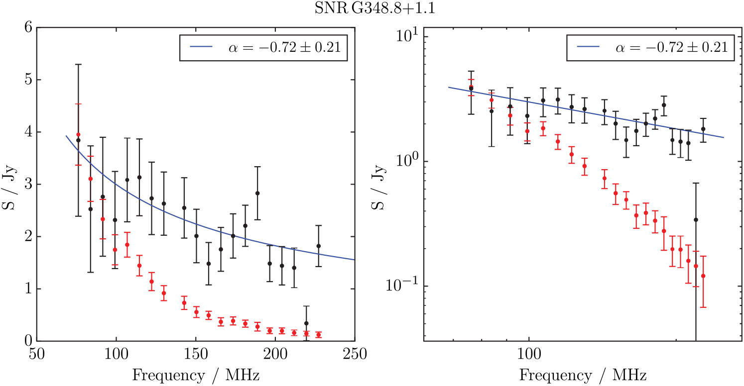
Spectral fitting over the GLEAM band for G352.2–0.1.
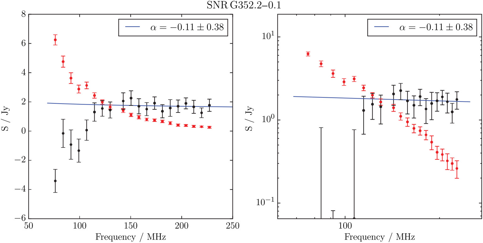
Spectral fit to the GLEAM and Parkes 2.4 GHz data integrated flux densities for SNR G353.3 – 1.1. Raw flux densities are shown with grey points; measured and extrapolated compact source flux densities are shown by green points, and the source-subtracted data (for ν > 150 MHz) used to fit the spectrum of the SNR are shown in black. As per the other plots, the fit is shown with a blue line.
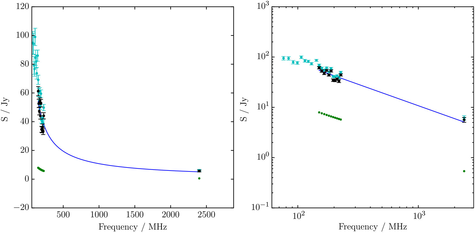
Spectral fitting over the GLEAM band for G354.46 + 0.07.
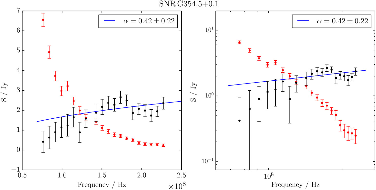
Spectral fitting over the GLEAM band for G356.6 + 00.1.
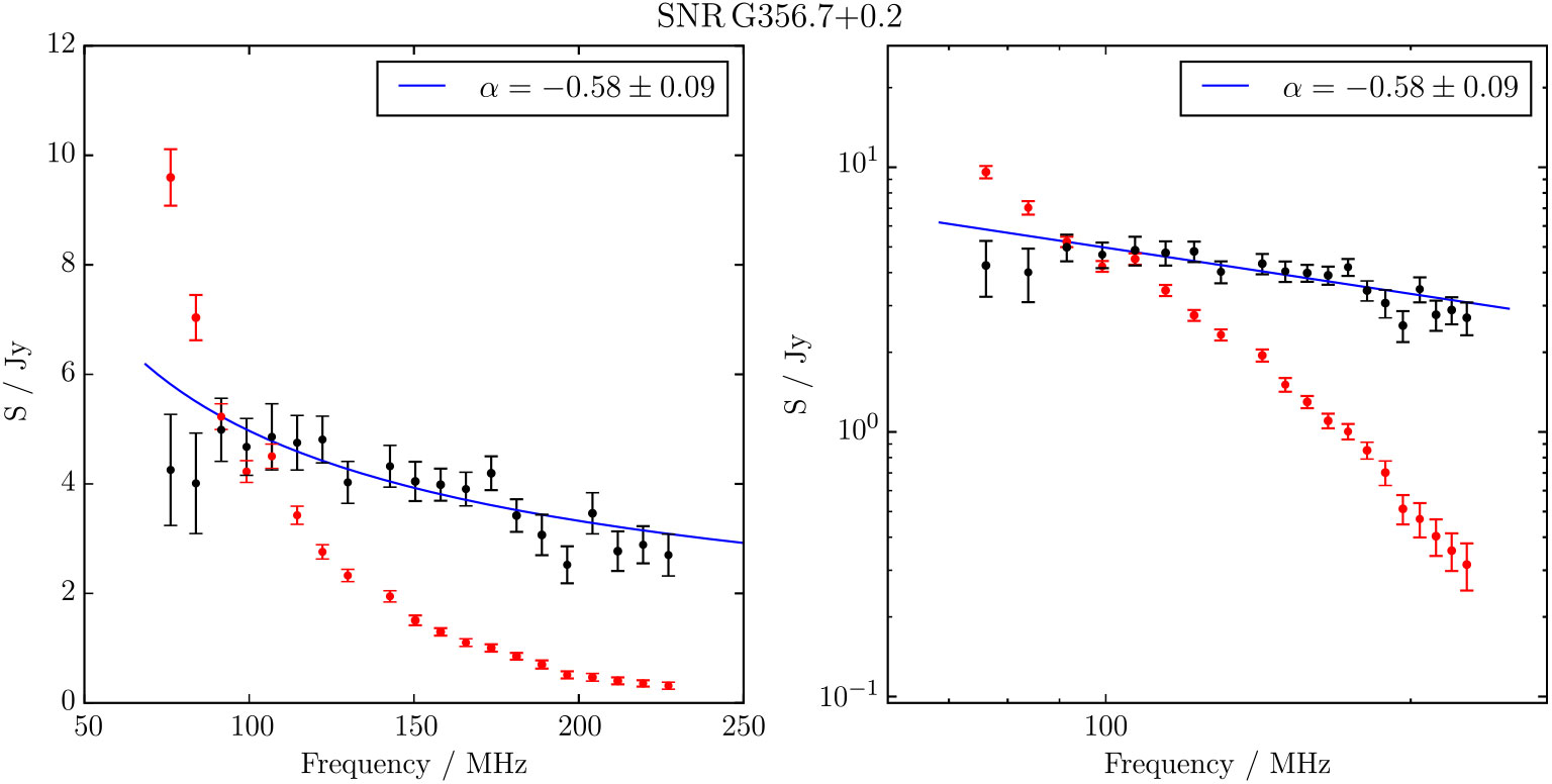
Spectral fitting over the GLEAM band for G359.2 –01.1.
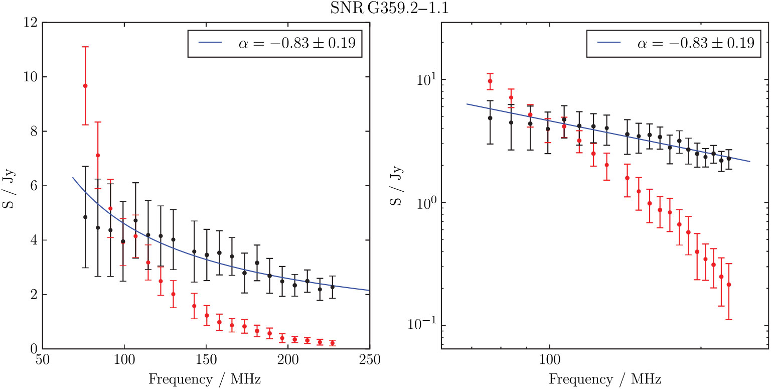
Spectral fitting over the GLEAM band for G3.1–0.7.
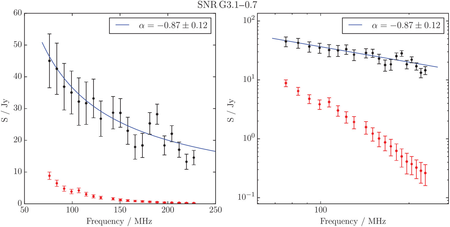
Spectral fitting over the GLEAM band for G7.5–1.7.
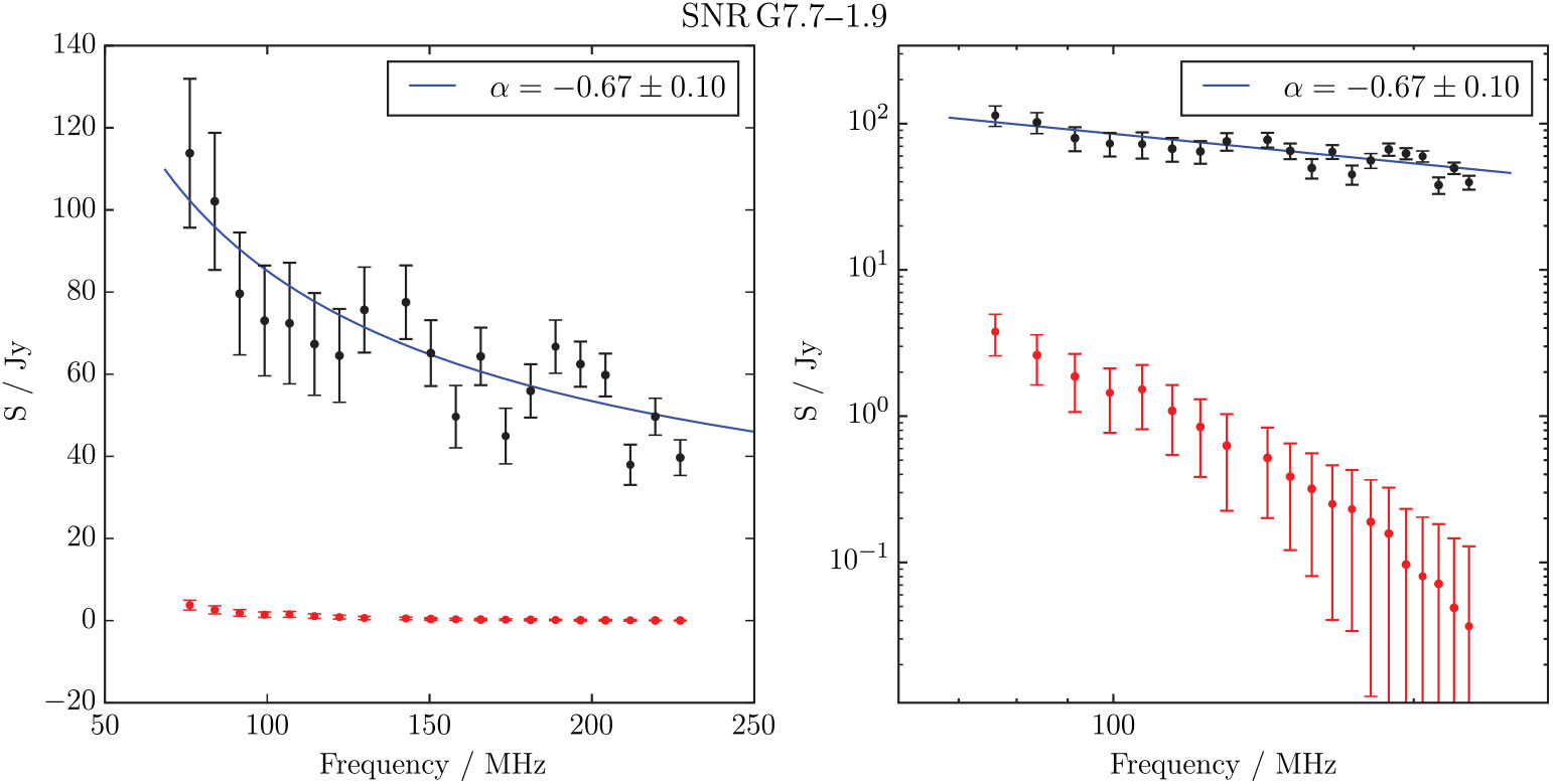
Spectral fitting over the GLEAM band for G13.1–0.5.
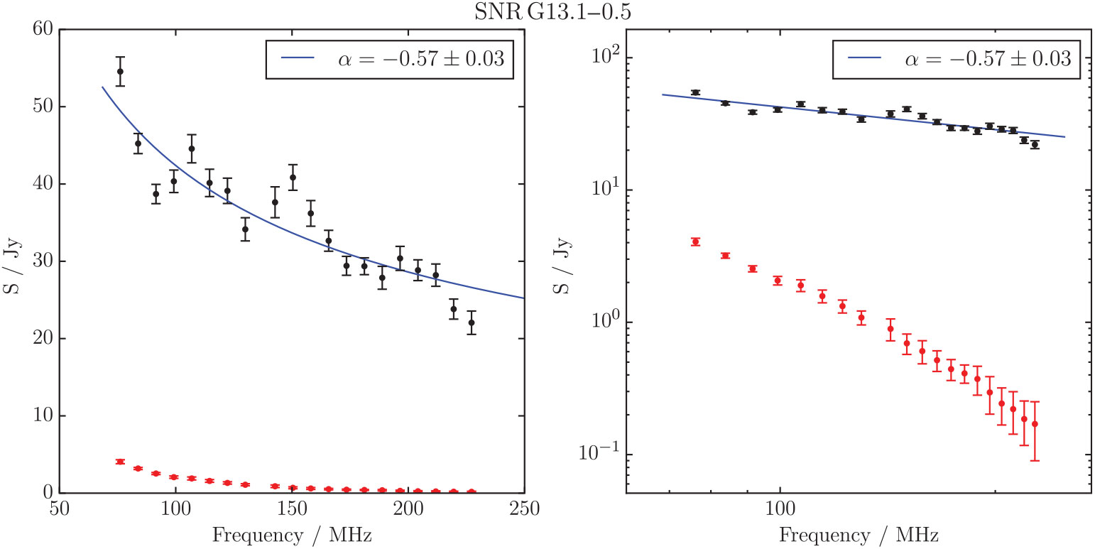
Spectral fitting over the GLEAM band for G15.51–0.15.
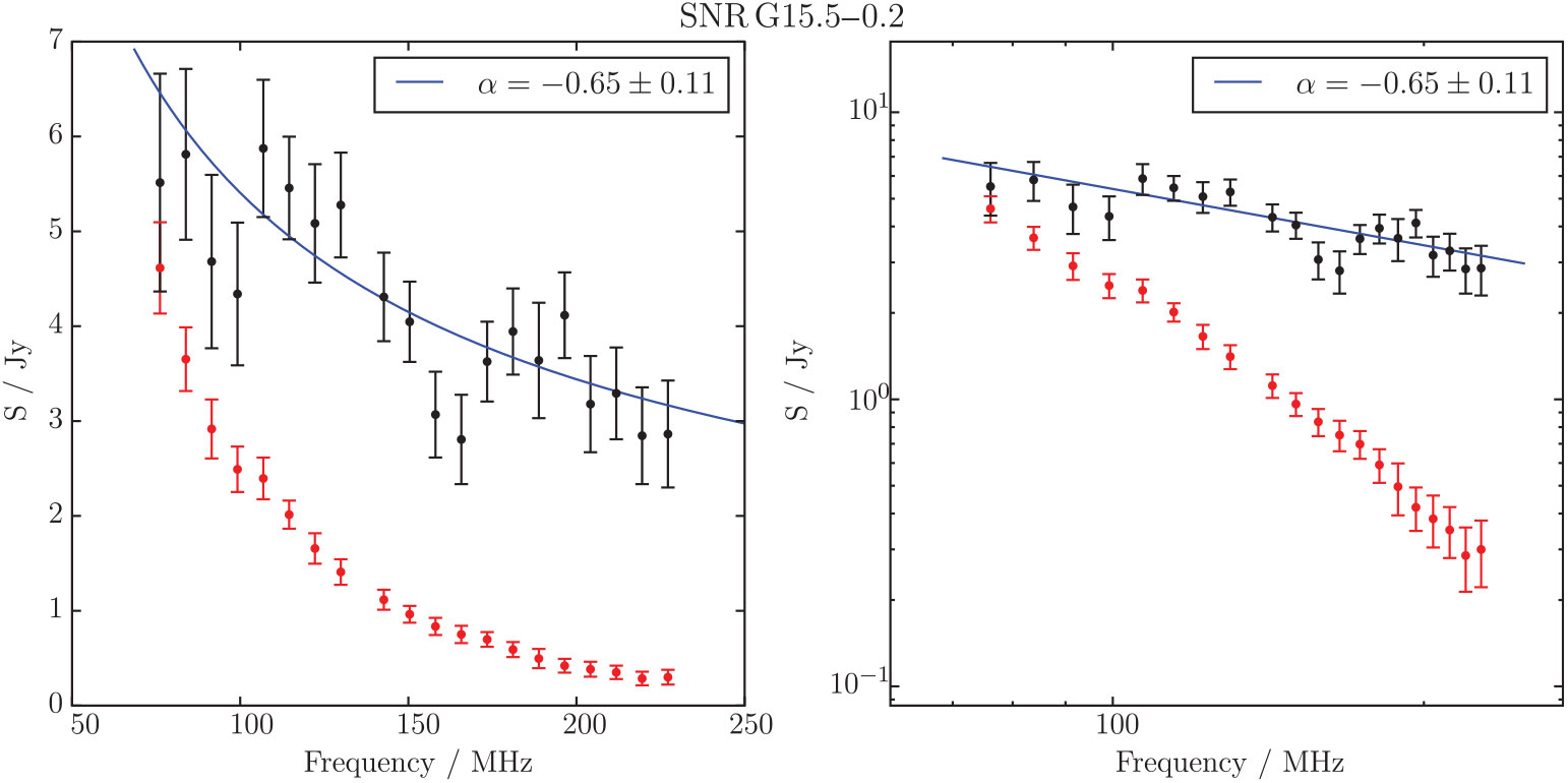
Spectral fitting over the GLEAM band for MAGPIS 9.6833 − 0.0667.
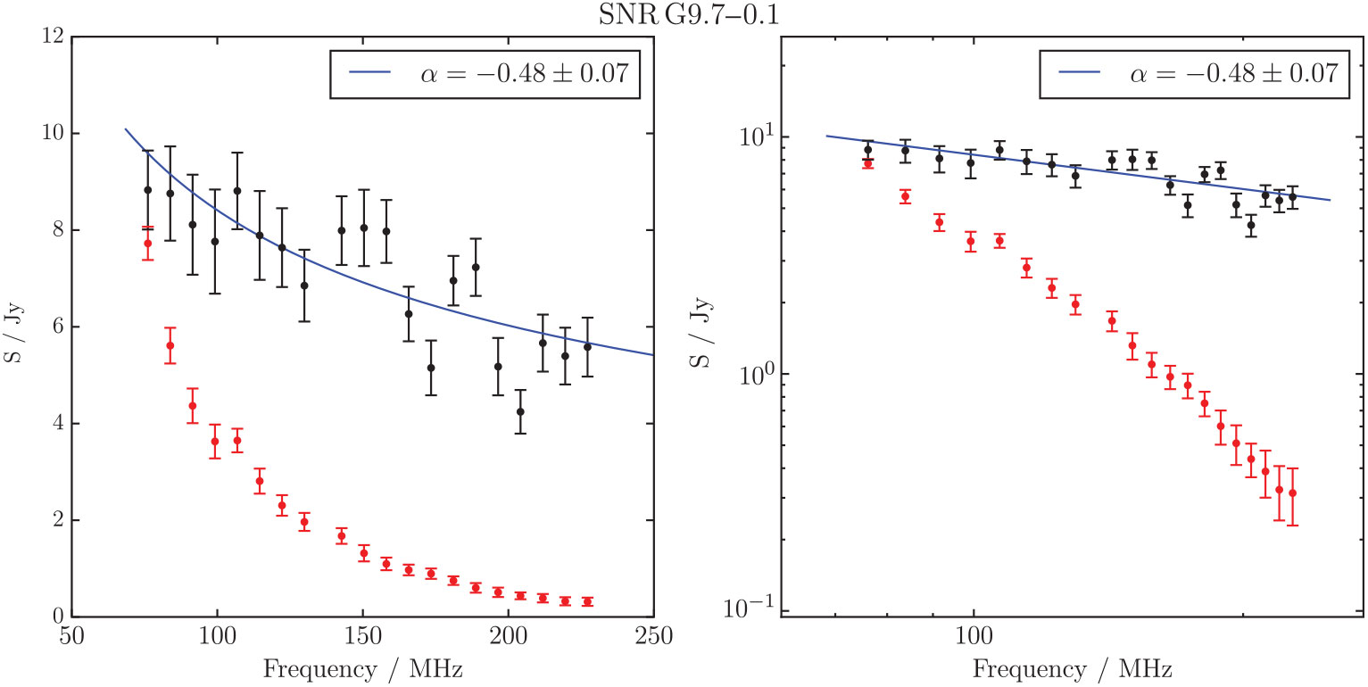
Spectral fitting over the GLEAM band for MAGPIS 28.3750 + 0.2028.
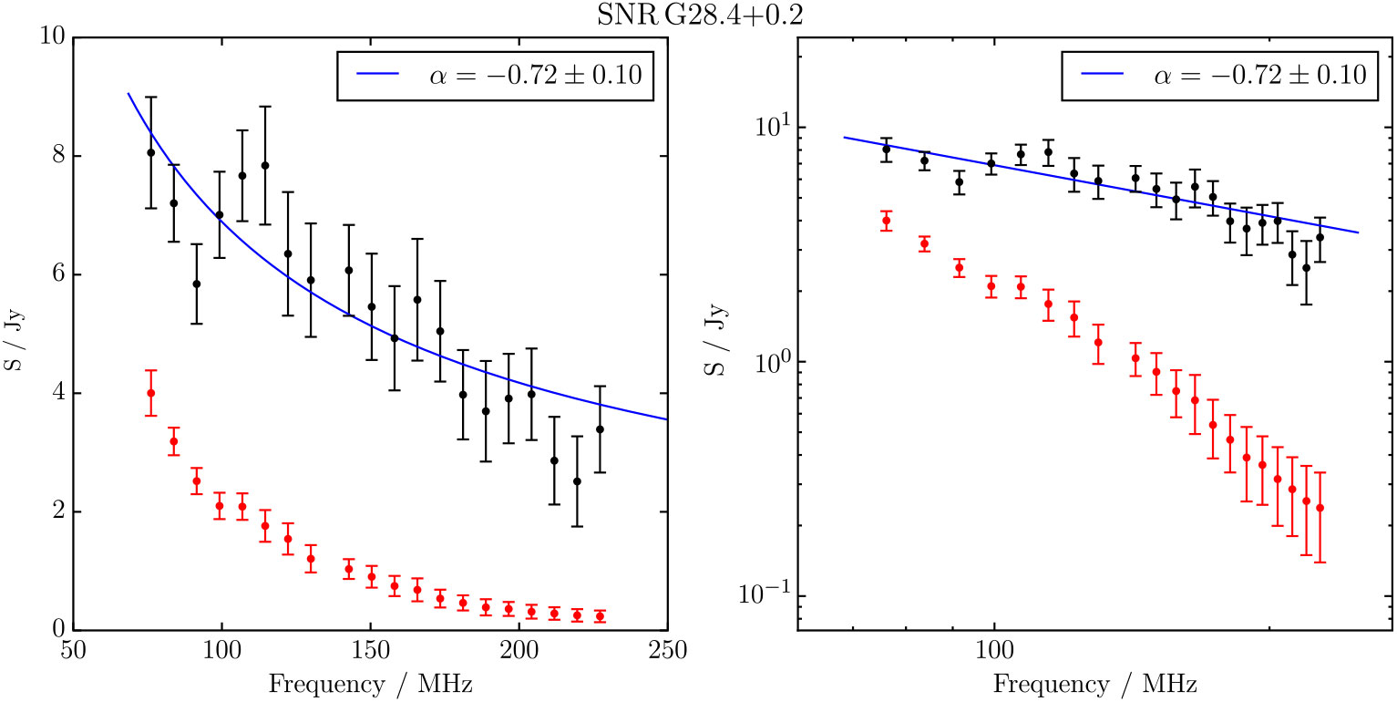
Spectral fitting over the GLEAM band for MAGPIS 28.7667 – 0.4250.
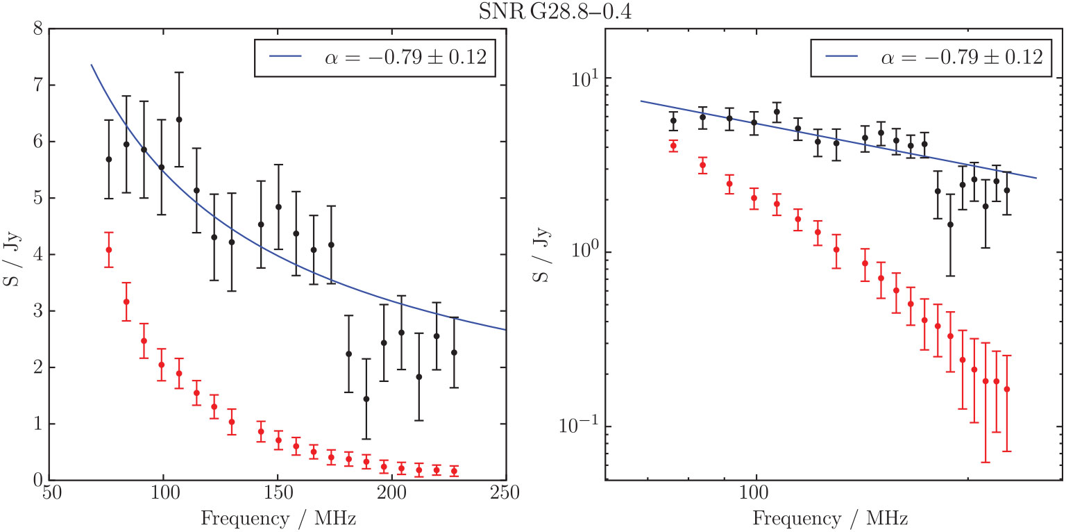
Spectral fitting over the GLEAM band for MAGPIS 27.1333 + 0.0333.
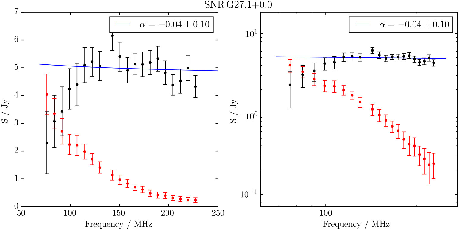
Spectral fitting over the GLEAM band for MAGPIS 20.4667 + 0.1500.