

1. INTRODUCTION
Ogives remain one of the most enigmatic features of glacier flow. In the mid-19th century, the pioneers of glaciology showed a keen interest in these natural features which could be easily seen from remote observation sites (Agassiz, Reference Agassiz1840; Forbes, Reference Forbes1845). Band ogives consist of alternating light and dark bands. Band ogives are ~30–50 m wide in the ice flow direction (Reynaud, Reference Reynaud1979).They are also referred to as Forbes bands, named after the physicist who first described the phenomenon on the Mer de Glace glacier in France (Forbes, Reference Forbes1845). These band ogives should not be confused with wave ogives which are surface undulations often found at the base of icefalls (Goodsell and others, Reference Goodsell, Hambrey and Glasser2002). Wave ogives result from a combination of variations in ablation and plastic deformation occurring through icefalls (Nye, Reference Nye1958; Waddington, Reference Waddington1986).
1.1. Band ogives theories
Several theories have been proposed for the genesis of band ogives (e.g. Forbes, Reference Forbes1845; Haefeli, Reference Haefeli1951; King and Lewis, Reference King and Lewis1961; Vallon, Reference Vallon1967; Posamentier, Reference Posamentier1978; Reynaud, Reference Reynaud1979; Lliboutry and Reynaud, Reference Lliboutry and Reynaud1981; Goodsell and others, Reference Goodsell, Hambrey and Glasser2002). The reason for the color difference in band ogives is a highly contentious issue (Goodsell and others, Reference Goodsell, Hambrey and Glasser2002).
Some authors suggest that the darker bands are caused by dirt that comes from the surface and accumulates more readily in the troughs of wave ogives (Allen and others, Reference Allen, Kamb, Meier and Sharp1960; King and Lewis, Reference King and Lewis1961; Atherton, Reference Atherton1963). Other studies indicate that the dirt originates from within the ice, with the dark ogive zones being richer in englacial debris (Haefeli, Reference Haefeli1951; Leighton, Reference Leighton1951; Posamentier, Reference Posamentier1978). Several authors noticed that the darker bands consist of coarse, bubble-free blue ice while the light bands consist of bubble-rich white ice (Fisher, Reference Fisher1962; Vallon, Reference Vallon1967; Posamentier, Reference Posamentier1978; Reynaud, Reference Reynaud1979; Lliboutry and Reynaud, Reference Lliboutry and Reynaud1981; Goodsell and others, Reference Goodsell, Hambrey and Glasser2002). According to these studies, the color differences result from differences in ice type. Vallon (Reference Vallon1967) pointed out that cryoconite and other debris remain preferentially close to the surface of the bubble-free ice. In contrast, cryoconite and dirt penetrate more easily in the bubble-rich ice, due to the strong albedo difference between the dirt and the white ice. Other authors suggest that the main cause of the brightness difference is related to the intensity of foliation (Posamentier, Reference Posamentier1978; Goodsell and others, Reference Goodsell, Hambrey and Glasser2002). The difference in foliation leads to differential weathering and the presence of small-scale weathered ridges trapping dirt more effectively on the dark foliated areas (Posamentier, Reference Posamentier1978; Goodsell and others, Reference Goodsell, Hambrey and Glasser2002).
Guy and others (Reference Guy, Daigneault and Thomas2002) suggested that band ogives result from a self-organization. According to this theory, the alternating dark and light bands originates from a combination of higher internal melt in dark bands and a lower melt in light bands. The dark bands would be due to a local increase in the mineral content which leads to a lowering of the temperature and pressure of ice melting, and an increase of dust content within the ice. It would be followed by a decrease in pressure that can stop the melt, creating a light band (Guy and others, Reference Guy, Daigneault and Thomas2002).
In addition to the origin of the color difference, important questions arise concerning the genesis of the bubble-rich white ice and the bubble-free blue ice.
1.2. Band ogives and the presence of an icefall
Most of the studies suggest that the genesis of band ogives requires the presence of an icefall upstream (King and Lewis, Reference King and Lewis1961; Fisher, Reference Fisher1962; Vallon, Reference Vallon1967; Posamentier, Reference Posamentier1978; Reynaud and others, Reference Reynaud1979; Lliboutry and Reynaud, Reference Lliboutry and Reynaud1981; Goodsell and others, Reference Goodsell, Hambrey and Glasser2002) with an extensive flow in the icefall followed by a compressive flow at the foot of the icefall. Two very different assumptions explain the alternating dark and light bands. On one hand, Nye (Reference Nye1958); King and Lewis (Reference King and Lewis1961); Vallon (Reference Vallon1967); Lliboutry and Reynaud (Reference Lliboutry and Reynaud1981) and Fisher (Reference Fisher1962) suggest that the rapid ice velocity of the icefall allows a parcel of ice to pass through the icefall each summer and winter. They consider that dark bands are formed by the concentration of debris and refrozen water in glacier-wide crevasses during the summer (King and Lewis, Reference King and Lewis1961; Vallon, Reference Vallon1967; Reynaud, Reference Reynaud1979; Lliboutry and Reynaud, Reference Lliboutry and Reynaud1981). Reynaud (Reference Reynaud1979) and Lliboutry and Reynaud (Reference Lliboutry and Reynaud1981) note that thanks to crevasses, blue ice and dust penetrate down to about two-thirds of the glacier thickness at Mer de Glace glacier. In contrast, the light bands are considered to result from the winter snowfalls which form the bubble-rich white ice. On the other hand, Posamentier (Reference Posamentier1978) suggested that the dark bands result from bubble-free and debris-rich ice which is transported upward, from near the glacier base to the surface, by the processes of folding and potentially reverse faulting due to compressive flow at the base of the icefall. According to this hypothesis, the basal ice is uplifted to the glacier surface to produce the dark foliated band ogives. Goodsell and others (Reference Goodsell, Hambrey and Glasser2002) confirmed this theory by analyzing ice samples extracted from the surface of the dark bands at Bas Glacier d'Arolla (Switzerland). The debris content was shown to come for the glacier base. Their model is a variation of reverse faulting with associated drag folding (Posamentier, Reference Posamentier1978), although they mention that the drag folding hypothesis is not required for Bas Glacier d'Arolla. Goodsell and others (Reference Goodsell, Hambrey and Glasser2002) concluded that the band ogives result from sedimentary stratification and crevasse traces which have been transposed into arcuate, transverse foliation. They suggest that the folds become tighter down-glacier as a result of longitudinal compression, before becoming an integral part of the foliation.
Several of these theories suggest a difference in ice ablation between dark and light ogives (Posamentier, Reference Posamentier1978; Goodsell and others, Reference Goodsell, Hambrey and Glasser2002; Guy and others, Reference Guy, Daigneault and Thomas2002). However, to our knowledge, the ablation difference between dark and light ogives has never been established.
1.3. Objectives of this study
The goal of this paper is to investigate the rate and mechanisms of ice ablation both on dark and light band ogives based on albedo and surface roughness measurements and surface mass balance (SMB) modeling. For this purpose, our paper aims at (i) comparing the ice ablation observed over 12 years on dark and light ogives and (ii) understanding the prevailing processes which drive ice ablation on both types of ogives. Providing a general theory for band ogive formation is beyond the scope of this study.
2. STUDY SITE, DATA AND METHODS
2.1. Study site and description of Forbes bands
The Mer de Glace glacier (45°55′N, 6°57′E) is the largest glacier in the French Alps, covering a surface area of 28 km2 between 4300 and 1600 m a.s.l.
Alternating light and dark bands can be seen on the Mer de Glace glacier downstream from the ‘Séracs du Géant’ icefall. Wave ogives first appear at the foot of the icefall. These wave ogives are smoothed out with distance from the icefall.
The color difference between light and dark bands does not fully develop until some distance downstream from the foot of the icefall, once the wave topography has been reduced. The enhanced color differentiation coincides with the declining amplitude of the wave ogives as seen on the Bas Glacier d'Arolla (Goodsell and others, Reference Goodsell, Hambrey and Glasser2002).
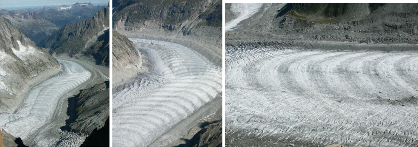
Our study focuses on a small part of Mer de Glace, in the ablation zone, named ‘Tacul glacier’, on which dark and light ogives are clearly visible (Figs 1, 2). This zone is ~2 km downstream from the icefall. We selected a small area of ~1800 m2 at 2100 m a.s.l. on the Tacul glacier, and performed point annual mass-balance measurements between 2004 and 2015 using six stakes inserted in the ice. The ice flow velocity is ~50 m a−1 in this area (Berthier and Vincent, Reference Berthier and Vincent2012; Vincent and others, Reference Vincent, Harter, Gilbert, Berthier and Six2014). The maximum ice thickness is 350 m. The glacier is ~800 m wide in this region.
Map of Tacul glacier located downstream from the icefall. The ablation stakes set up in dark and light band ogives are indicated in red. Some crevasses located at the foot of the icefall can be seen at the bottom of the figure. The image is from a 2008 orthophoto (Régie de Gestion des Données 73–74). The contour interval is 10 m.

Pictures of Forbes bands at the Mer de Glace glacier (2004). In the image on the right, the glacier flows from right to left.
2.2. Point mass balance and ice flow velocity measurements
Each year between 2004 and 2015, three stakes were set up in a dark ogive and three others in the next upstream light ogive. Given that the ogives move with the glacier, the stakes were not set up exactly at the same locations every year. Geodetic measurements were performed to obtain the coordinates of the ablation stakes at the end of each summer. For this purpose, we used a Leica 1200 Differential GPS (DGPS) unit, running with dual frequencies. Occupation times were typically 1 min with 1-s sampling and the number of visible satellites (GPS and GLONAS) was greater than seven. The distance between the fixed receiver and the mobile receiver was 2 km. The DGPS positions have an intrinsic accuracy of ±0.01 m. However, depending on the size of the holes drilled to insert the stakes, the stake positions have an uncertainty of ±0.05 m.
The winter mass balances were measured at the end of April using snow cores and density measurements. During the ablation season (April–October), the sites were visited monthly. The summer mass balance is calculated from the difference between the winter mass balance and the annual mass balance. The uncertainties of the direct measurements have been assessed at ~0.20 m w.e. a–1 for winter mass balances and 0.15 or 0.30 m w.e. a–1 for summer mass balances, depending on whether the ablation concerned ice or snow and firn (Thibert and others, Reference Thibert, Blanc, Vincent and Eckert2008). Given that our measurements are performed in the ablation zone, the annual mass-balance observations performed in September or October result from emergence stakes set up in ice. Consequently, the uncertainty of the emergence measurements does not exceed 0.15 m w.e. a–1. Another source of uncertainty could be related to the influence of compressive or extensive flow which can lead to errors in the determination of ablation using stakes, as shown by Vallon (Reference Vallon1968). Vallon (Reference Vallon1968) recommends a correction for regions of high extensive or compressive flow. The ice flow velocities observations performed in the studied area (Berthier and Vincent, Reference Berthier and Vincent2012) reveal a compressive flow in this region with a horizontal strain rate close to −0.015 a−1. Given that the buried length of each stake is ~7 m on average during the whole year, this correction should not exceed 0.10 m w.e. a−1.
2.3. Spectral albedo measurements
To investigate the difference in albedo between the dark and the light ogives, we performed spectral albedo measurements using the solalb instrument at each stake and between stakes with a spatial sampling distance varying from 15 to 40 m (17 locations are used in the following). The instrument is a one-channel version of the spectrometer described in Libois and others (Reference Libois2015); Picard and others (Reference Picard, Libois, Arnaud, Verin and Dumont2016a) and Dumont and others (Reference Dumont2017). Spectral albedo is obtained by two successive measurements of the radiation with the light collector looking upward and downward. The spectrometer has a range 400–1050 nm and an effective resolution of 3 nm. Each measurement was performed ~1 m above the ice surface. The accuracy of the sensor leveling was better than 1°.
Sky conditions were not perfectly stable over the time period of the measurements (13 July 2015, from 11:00 to 14:00 local time), leading to some spectra measured under clear sky conditions and others under overcast conditions. The stability of the integrated incident radiation was monitored during successive acquisitions, allowing us to immediately discard any albedo measurements with variations larger than 2%.
Following Picard and others (Reference Picard, Arnaud, Panel and Morin2016b), every raw spectrum was processed to take into account (i) dark current and stray light, (ii) integration time scaling and (iii) collector angular response. The bi-hemispherical reflectance (Schaepman-Strub and others, Reference Schaepman-Strub, Schaepman, Painter, Dangel and Martonchik2006), referred to as ‘spectral albedo’ in the following, was obtained as the ratio between the upward and downward acquisitions. Note that the collector angular response correction requires the proportion of diffuse and direct irradiance. This was obtained using SBDART simulations (Ricchiazzi and others, Reference Ricchiazzi, Yang, Gautier and Sowle1998), considering clear-sky and a typical winter temperate region atmosphere. SBDART spectral irradiance estimates were also used to calculate broadband albedo from the spectral albedo values.
Note that since the measurements were performed 1 m above the surface, the albedo value corresponds to a surface effective albedo value on a 300 m2 footprint and accounts for the effect of surface roughness (Cathles and others, Reference Cathles, Abbot, Bassis and Macayeal2011; Lhermitte and others, Reference Lhermitte, Abermann and Kinnard2014).
2.4. DGPS and photogrammetry measurements
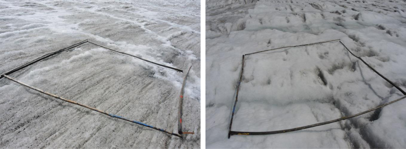
A terrestrial photogrammetric survey was carried out on 11 August 2016. We acquired 30 and 34 terrestrial photographs for the light and dark ogives, respectively. The photographs were taken using a Nikon Coolpix P7700 digital camera at a distance of ~4 m, thereby covering a surface area of ~5 m2 for each ogive (Fig. 3).
Dark (left) and light (right) ogives. The stakes are 2 m long (Photo C. Vincent, 2016).
The images from the survey were processed using the Structure for Motion (SfM) algorithm implemented in the Agisoft Photoscan Professional version 1.2.0 software package (Agisoft, 2014).
In order to georeference the surface models and to geometrically correct the images, ten ground control points (GCPs) (0.1 × 0.1 m white crosses painted on pieces of wood) were set up for each sampled area. These GCPs, easily identifiable on the pictures, were measured using a geodetic DGPS. The SfM stereo technique was then used to generate a dense point cloud of the glacier surface. All processing parameters were set to ‘high quality’ in the Agisoft Photoscan software. This dense point cloud was used to construct the DEMs. Photogrammetric restitutions were obtained with marker residuals of 0.01 and 0.03 m for the dark and the light ogives, respectively. A detailed description of the processing steps can be found in Kraaijenbrink and others (Reference Kraaijenbrink, Immerzeel, Pellicciotti, de Jong and Shea2016) or Brun and others (Reference Brun2016).
The positions of all GCPs used for the photogrammetric survey were measured with a Leica 1200 DGPS unit. Occupation times were 1 min with 1 s sampling and the number of visible satellites (GPS and GLONAS) was greater than seven. The distance between the fixed receiver and the mobile receiver was 2 km. In order to improve the relative accuracy between GCPs, we set up a second fixed receiver close to the measurement areas, i.e. ~40 m away. The position of the second receiver was consequently obtained accurately from an occupation time of 8 h and the positions of the mobile receiver were calculated from this second receiver. Furthermore, in order to improve the accuracy, the height of the antenna used for GCPs measurements was 10 cm. Thus, the GCPs have an accuracy of ±0.005 m. In addition, two longitudinal profiles were measured on dark and light ogives, respectively, from DGPS measurements at ~10 cm intervals.
2.5. Surface roughness
The aerodynamic roughness length z 0 is defined as the height above the ground at which a vertical wind profile drops to zero for a logarithmic profile (Oerlemans, Reference Oerlemans2001; Greuell and Genthon, Reference Greuell, Genthon, Bamber and Payne2004). Here we estimate the effective roughness length z 0 and assess the impact on the energy balance of both ogives. Previous studies attempted to estimate z 0 using a microtopographic method (e.g. Lettau, Reference Lettau1969; Munro, Reference Munro1989; Brock and others, Reference Brock, Willis and Sharp2006; Irvine-Fynn and others, Reference Irvine-Fynn, Sanz-Ablanedo, Rutter, Smith and Chandler2014; Rounce and others, Reference Rounce, Quincey and McKinney2015). Traditional microtopographic methods rely on measurements of elevation along a transect. More recently, close-range accurate photogrammetry was used (Irvine-Fynn and others, Reference Irvine-Fynn, Sanz-Ablanedo, Rutter, Smith and Chandler2014). Here we used DEMs with a grid size of 1 cm, determined from numerous terrestrial photographs using Agisoft Photoscan software.
Numerous relationships between surface roughness element geometry and z 0 have been proposed. Conventional microtopographic techniques to estimate z 0 are based on Lettau (Reference Lettau1969):
 $$z_0 = \sigma _{\rm h}s/S$$
where σ h is half the effective roughness element height or half the average vertical extent, s the typical roughness element silhouette area or vertical crosswind-lateral plane and S the specific area measured in the horizontal plane or the density of roughness elements (Munro, Reference Munro1989; Brock and others, Reference Brock, Willis and Sharp2006).
This equation can be simplified (Brock and others, Reference Brock, Willis and Sharp2006; Irvine-Fynn and others, Reference Irvine-Fynn, Sanz-Ablanedo, Rutter, Smith and Chandler2014) and rewritten as:
 $$z_0 = (\sigma _{\rm h})^{\rm 2}f/L$$
where f is the number of groups of positive deviations above the zero mean across the profile over length L.
2.6. SMB simulations
SMB simulations were performed using the SURFEX/ISBA-Crocus detailed snowpack model (Brun and others, Reference Brun, David, Sudul and Brunot1992; Vionnet and others, Reference Vionnet2012), hereafter referred to as Crocus. An exhaustive description of the model is provided in Vionnet and others (Reference Vionnet2012). Crocus is a full energy-balance model using a layered Lagrangian representation of the snowpack. Each layer is defined by its physical properties (snow morphological parameters, enthalpy, density and thickness). In the model, any snow layer with a density >850 kg m−3 is considered as ice. Crocus is a 1D model implying that any lateral flux is neglected. This is not a limitation in the snowpack and in the ice because the glacier is temperate, that is, its temperature is almost uniform. In the atmosphere, we perform independent 1-D simulations on each ogive as if they were horizontally infinite.
2.6.1. Crocus albedo scheme
The original Crocus albedo scheme uses three spectral bands for albedo and solar energy extinction calculations (0.3–0.8, 0.8–1.5 and 1.5–2.8 µm). For each band, the snow albedo and the absorption coefficient is parameterized as a function of the snow grain parameters and the age and density of the snow layer for the absorption coefficient.
If the density of the snow layer is higher than 850 kg m−3, the albedo and absorption coefficients are set to constant values that can be assigned by the user (see Vionnet and others, Reference Vionnet2012 for more details).
2.6.2. Crocus turbulent fluxes scheme
Crocus uses a bulk formulation for the estimation of the turbulent latent and heat fluxes which relies on the calculation of a turbulent exchange coefficient determined by an effective aerodynamic roughness length, z 0.
Crocus surface turbulent fluxes are proportional to the turbulent exchange coefficient or drag coefficient C H, which depends on the Richardson number, R i and on the effective roughness length for momentum, z 0 and for heat, z 0H (Noilhan and Mahfouf, Reference Noilhan and Mahfouf1996). R i quantifies the stability of the atmosphere above the snow or the ice surface. To ensure a minimal level of turbulence in stable conditions due to complex topography of mountain terrain, a threshold value of 0.2 is applied to the Richardson number (Vionnet and others, Reference Vionnet2012). z 0H is calculated as z 0/10 (Vionnet and others, Reference Vionnet2012).
The default values for z 0 over snow and ice are usually 1 and 10 mm, respectively (see Vionnet and others, Reference Vionnet2012 for more details). Note that the relationship between this effective roughness length and a geometrical roughness length is not straightforward. In the following, this parameter is referred as to roughness length.
2.6.3. Input meteorological data
In this study, we used meteorological driving data from the SAFRAN system (Système d'Analyse Fournissant des Renseignements Adaptés à la Nivologie, system of analysis providing adapted information for snow studies, Durand and others, Reference Durand2009). The system performs a meteorological analysis based on the ERA-40 reanalysis and on observed weather data from the automatic weather and precipitation station conventional network of Météo-France in the French mountain ranges. However, the system is poorly constrained at high elevation sites such as Mer de Glace due to the limited number of observations available at such elevations.
The system provides hourly air temperature, specific humidity, precipitation rate and phase, downward longwave and shortwave radiation and wind speed data that are used as input for the snow model. Réveillet and others (Reference Réveillet, Vincent, Six and Rabatel2017) used the same set-up to simulate the SMB of Saint-Sorlin glacier (Grandes Rousses massif, French Alps) and they concluded that it was necessary to adapt the SAFRAN reanalysis at high elevations using automatic weather station measurements (AWS). In this study, we consequently use wind speed measurements from an automatic measurement station located on the Argentière glacier moraine that is operated in the framework of the GLACIOCLIM observatory. The station is located at 45°58′2.70″N, 6°58′35.56″E, at an elevation of 2450 m a.s.l. Although the AWS is 8 km from the stakes, we assume that the measured wind speed is more representative of Mer de Glace conditions than SAFRAN outputs that do not account for topographic effects and are the only representative of the synoptic conditions. The comparison between SAFRAN and AWS wind speed shows that SAFRAN wind speed is generally lower by 1–2 m s−1 than the AWS wind speed. Note that these data are only available from 1 August 2006. In addition, winter precipitation used in Crocus was adjusted to fit the winter mass-balance measurements at each stake. The adjustment was performed using a multiplication factor on the solid precipitation amount during the accumulation period for each stake location and each year. The multiplication factor was selected so that the RMSE between simulated and measured winter mass balance was smaller than 0.2 m w.e., i.e. smaller than the uncertainties of the winter mass-balance measurements. Lastly, shadowing effects on shortwave radiation due to adjacent slopes were taken into account in the simulations. The shadowing mask was calculated based on a 25 m spatial resolution DEM from IGN (BD ALTI®), available at http://professionnels.ign.fr/bdalti.
2.6.4. Simulation set-up
Mass-balance simulations were performed from 1 August 2006 to 1 November 2015. We initialized the simulations with a 45 m column of ice and no snow and we performed a 7-year spin up to adjust ice temperature. The simulations were performed at the location of the three stakes in the light ogives using ice albedo values derived from albedo measurements, called α light hereafter (see Section 2.3), and at the locations of the three stakes located in the dark ogives using α dark albedo values also derived from in situ measurements. We consequently made the very simplistic assumption that ice albedo values do not change significantly during summer and between years. The sensitivity of the simulations to the value of the effective roughness length z0 is investigated in the next section.
3. RESULTS
3.1. SMB on light and dark ogives over 12 years of observations
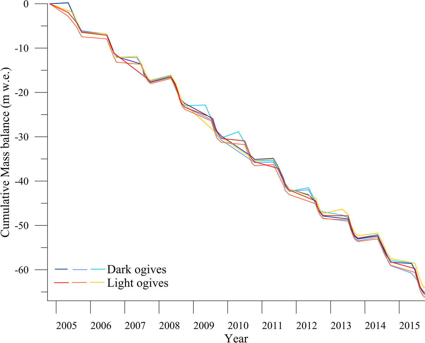
Cumulative measured mass balances were obtained for the six ablation stakes, three of them set up in the dark band and the three others in the light band (Fig. 4). Between 24 October 2004 and 28 September 2015, the cumulative mass balance ranges between −64.1 and −66.2 m w.e. for both groups of stakes set up on dark and light ogives. This corresponds to a difference of 0.19 m w.e. a−1, which is almost within the uncertainty. Note that no systematic differences in ablation are observed between stakes set up in dark and light ogives. Indeed, the maximum ablation was reached for two stakes, one in the dark ogive and the other in the light ogive. The winter accumulation was measured at each stake for each winter except for some years. Although the stakes were only ~30 m apart, differences in accumulation could explain part of the small differences between annual mass balances. In any case, these observations show that the measured SMB is very similar to dark and light ogives.
Cumulative surface mass balances measured for the six ablation stakes set up in dark and light ogives over 2004–15.
3.2. Surface albedo difference between dark and light ogives
Figure 5 sums up all the albedo measurements performed in the dark and light ogives (top) and the spectral Std dev. of the albedo for the two types of ogives (bottom) calculated over all the measurements (nine for the light ogives and eight for the dark ogives).
Top: Summary of all the measured albedo values recorded for the light (deep and light blue lines) and the dark (black and grey lines) ogives. The sky conditions are indicated by the different colors. The thick blue and sand lines correspond to the mean spectra for the light and dark ogives. Bottom: The spectral Std dev. of the measured spectra for the dark (sand line) and the light (blue line) ogives.

As expected, the albedo measurements reveal a strong difference between the dark and light ogives.
It also shows that the variability of the albedo is slightly larger in the light ogives than in the dark ogives.
Using the mean spectral albedo for the light and dark ogives, respectively (thick lines in Fig. 5, top) and the spectral diffuse to total irradiance ratio obtained for Mer de Glace atmospheric conditions and 50° solar zenith angle, we calculated that the albedo for the 400–800 nm band is 0.373 ± 0.035 (resp. 0.200 ± 0.03) for the light (resp. dark) ogives. Within the 800–1000 nm band, the albedo of the light ogives is 0.223 ± 0.022, compared with 0.125 ± 0.015 for the dark ogives. For both types of ogives, the differences in band albedo are higher than the spectral variability within each type. This roughly corresponds to a difference in broadband albedo (400–2500 nm) of 0.13.
Consequently, the absorbed shortwave radiation is higher on the dark than on the light ogives, which should lead to higher ice ablation. Since we found similar ablation on dark and light ogives, another process must be present to compensate for the difference of absorbed short-wave energy.
3.3. Surface roughness difference
The turbulent exchanges of sensible and latent energy at a surface strongly depend on the aerodynamic roughness length z0 (e.g. Reid and Brock, Reference Reid and Brock2010; Irvine-Fynn and others, Reference Irvine-Fynn, Sanz-Ablanedo, Rutter, Smith and Chandler2014; Smith and others, Reference Smith2016).
From DEMs obtained using the SfM algorithm (Fig. 6), we selected 30 cross sections for each band ogive and calculated the roughness z 0 according to the study of Irvine-Fynn and others (Reference Irvine-Fynn, Sanz-Ablanedo, Rutter, Smith and Chandler2014). An example is given in Figure 7 for both dark and light bands. On the average, over the 60 cross sections, our results show large differences in z0, i.e. 2.9 mm ± 0.12 mm on the light band and 0.4 mm ± 0.20 mm on the dark band.
DEMs determined on light (left) and dark (right) bands using photogrammetric measurements. The contour interval is 0.01 m. The elevation scales are identical. The ground control points are shown in red. Note the ablation stakes (2 cm diameter) shown on the left side of each figure.

Cross sections through the light (left) and dark (right) ogives. Note that the vertical axis scales are the same. The red line corresponds to the zero mean across the profile over the length used in Eqn 2.
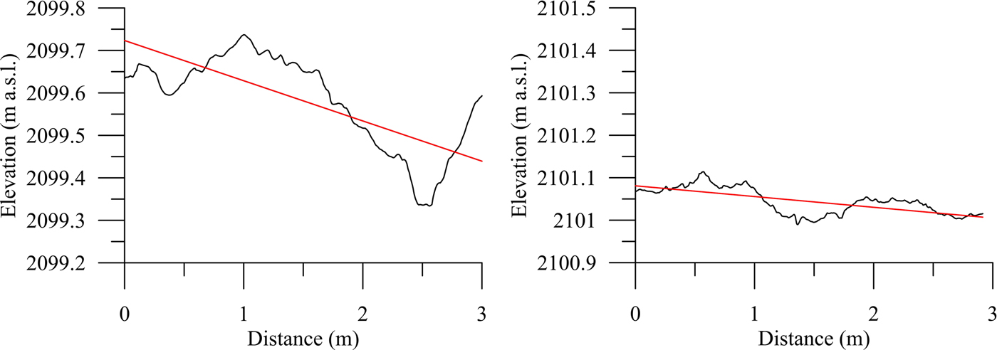
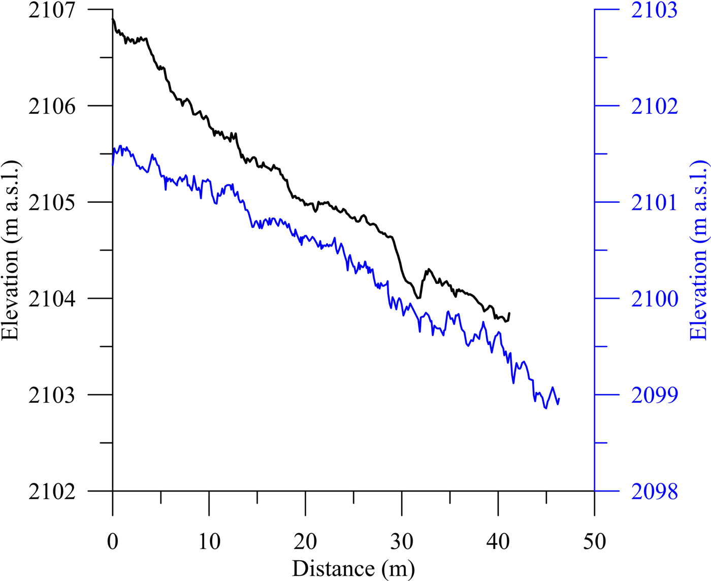
These values are consistent with those found in the literature for ice surfaces, generally in the range 0.1–6 mm (Brock and others, Reference Brock, Willis and Sharp2006; Smith and others, Reference Smith2016). Note that the value of z0 can reach 80 mm for very rough glacier ice (Smeets and others, Reference Smeets, Duynkerke and Vugts1999). The difference in roughness represents a factor of ~7 between the dark and light bands. In addition, these differences are obvious from longitudinal profiles measured at a spatial resolution of 10 cm from DGPS (Fig. 8) over a length of ~45 m. From these measurements, we can conclude that turbulent heat fluxes should be higher on light ogives than on dark ogives. Note that an order of magnitude change in z 0 leads to a factor of two in estimated turbulent fluxes change (Munro, Reference Munro1989; Hock and Holmgren, Reference Hock and Holmgren1996; Brock and others, Reference Brock, Willis and Sharp2006).
Cross sections measured on light (blue) and dark (black) ogives using DGPS measurements. Note that the vertical axes have the same scales.
3.4. Numerical modeling of the surface energy and mass balance on light and dark ogives
We used the Crocus model at the stake locations, forcing the albedo of ice to values measured in the field for the dark and light ogives. Figure 9 compares the simulated and observed cumulative mass balances from 2006 to 2015 obtained for several values of the effective roughness length.
Simulated (solid and dashed lines) and observed surface mass balances (markers). The only difference in the Crocus set-up between the black and the blue lines is the ice albedo.
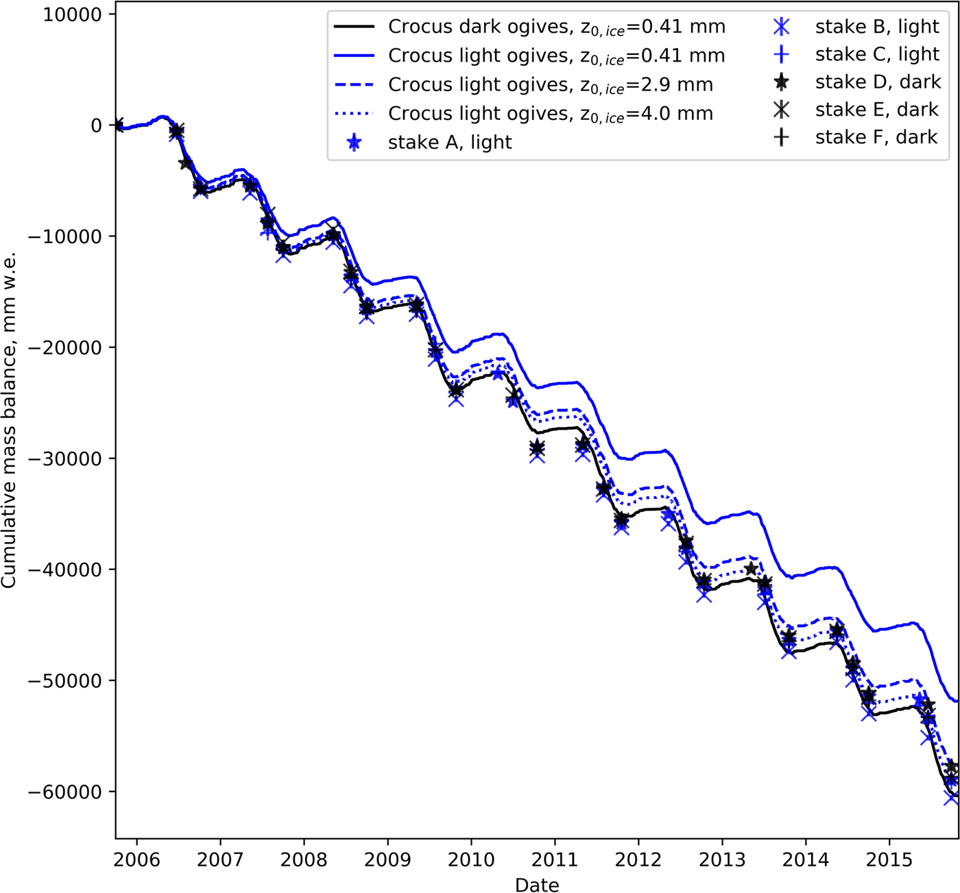
In the first modeling experiment, we used a unique value of roughness z 0 measured on the dark ogives (0.41 mm) for both dark and light bands when the surface was bare ice. When snow was present, all simulations used the default Crocus value (1 mm).
Figure 10 compares the measured and the simulated mass balances for two consecutive measurement dates (seasonal mass balance) for the light (upper panel) and the dark ogives (lower panel). For the dark ogives, only the results obtained with z 0 = 0.41 mm are shown while for the light ogives simulations results for z 0 = 0.41 mm and z 0 = 4.0 mm are reported.
Simulated versus measured mass balance (m w.e.) for the light ogives (upper panel, blue dots corresponds to the simulations with z 0 = 0.41 mm and green dots to the simulation with z 0 = 4.0 mm) and the black ogives (lower panel, simulations with z 0 = 0.41 mm). Each dot corresponds to the mass balance at one stake between two consecutive measurement dates shown on Figure 9. For each simulation, bias and RMSE are also indicated on figure.
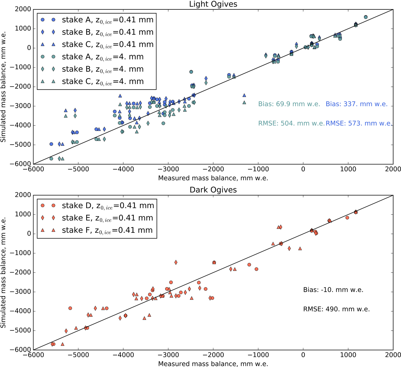
The results show that simulated mass balance agrees acceptably with the observed values for the dark ogives (RMSE: 0.490 m w.e., r 2 = 0.95) but are largely overestimated for the light ogives, when using z 0 = 0.41 mm (bias + 0.337 m w.e.). They also show that the difference in absorbed energy due to the difference in albedo would lead to a difference in ablation of ~9 m after 9 years without compensating processes.
In the second modeling experiment, we used the roughness values z 0 obtained from the field measurements, i.e. 0.41 and 2.9 mm, for dark and light bands, respectively. We then obtained a difference of 3.2 m w.e. in ablation between the dark and light ogives, which is 4.8% of the total measured ablation. This hardly exceeds the difference in ablation (2.1 m w.e.) between the maximum and minimum cumulative ablation measured on the stakes. In the third modeling experiment, we adjusted the roughness values z 0 of light bands in order to obtain similar ablation on both bands. The corresponding roughness value z 0 was 4.0 mm.
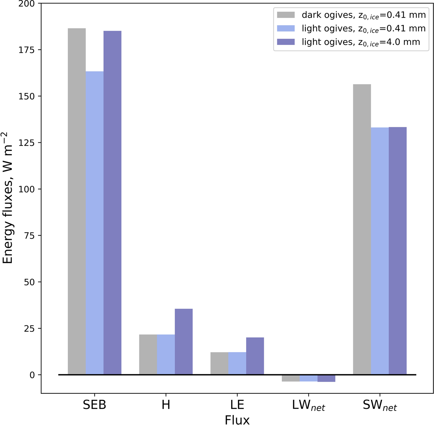
In addition, Figure 11 shows the simulated intensity of the different components of the surface energy balance (SEB) averaged from 2007 to 2015 for the period 1 June to 1 November each year. The figure displays the mean energy balance (SEB), the mean sensible (H) and latent (LE) heat fluxes, the net longwave radiation (downward-upward, LWnet) and the net shortwave radiation (SWnet) for the dark ogives in grey and for the light ogives (the two types of blue corresponding to two roughness lengths). It shows that over summer the energy balance is dominated by the SWnet term and that the dark ogives absorb on average 23 W m−2 more than the light ogives due to the albedo difference. The simulated total change in the turbulent fluxes (H + LE) due to the change in roughness length (from 0.41 to 4.0 mm) is able to compensate almost all this additional absorption (the difference between the gray and the dark blue energy balance is <2 W m−2).
Mean simulated energy balance for 1 June to 1 November of each year (2007–15 average). The different terms of the surface energy balance (SEB, sum of the four following terms) are the sensible (H), and latent (LE) heat fluxes, the net longwave radiation (downward-upward, LWnet) and the net shortwave radiation (SWnet). The gray bars correspond to the value simulated for the dark ogives with z 0 = 0.41 mm, the light blue bars to the values simulated for the light ogives with z 0 = 0.41 mm and the dark blue bars to the value simulated for the light ogives with z 0 = 4.0 mm.
4. DISCUSSION
4.1. Uncertainty on turbulent fluxes
In the numerical modeling experiments, the observed and calculated cumulative mass balances agree well when the measured roughness values are used for each band. The best agreement is achieved when using a roughness value of 4.0 mm for the light band instead of the measured value equal to 2.9 mm. However, the differences in cumulative mass balances obtained for both these values are within the uncertainty of the measured mass balance. In addition, the uncertainty of the measured roughness values is high. The difference between the adjusted value obtained from modeling (4.0 mm) for the light band and the measured value (2.9 mm) is within this uncertainty. Several alternative methods could be used for the calculations of z 0 (e.g. Smith and others, Reference Smith2016). Even if these alternative methods would lead to different absolute values of z 0, they would not change the strong difference in z 0 values found between dark and light bands given that the differences in the type of ice at the surface of the dark and light bands are similar whatever the calculation method (Smith and others, Reference Smith2016, Fig. 3a). Here, we found a factor of 7 difference between measured z 0 values for the dark and light bands. Taking into account the uncertainty of the measured z 0, this factor should be comprised between 3 and 19. Note also the large uncertainty in the turbulent exchanges calculations due to both the choice of the formulation and the uncertainty in the wind speed. In our study, the wind speed was obtained from the Argentière weather station located 8 km from our area study at 2430 m a.s.l. This may explain part of the uncertainties in the calculated turbulent fluxes.
It should be underlined that simulating snow and ice mass balance using detailed snowpack model is complex because of the high equifinality in the mass-balance calculation, i.e. the simulated mass balance may be accurate but for the wrong reasons (error compensation in the different components of the energy balance, e.g. Lafaysse and others, Reference Lafaysse2017). Snow/ice detailed modeling is generally affected by two sources of errors (i) uncertainties in the meteorological forcing data and (ii) errors and parameterizations in the physics of the snow/ice model itself. The use of another wind speed dataset or of another formulation of the turbulent fluxes will necessarily lead to different values of roughness length to minimize the SMB simulations errors. However, in light of this equifinality and uncertainties of roughness values, wind speed and turbulent fluxes formulation, the simulations shows that the sensible and latent flux increase due to increased surface roughness on light bands is likely the process which compensates for the net short-wave radiation increase related to the lower albedo observed on dark bands.
Another limitation of our calculation is the 1-D approach used for the calculation of the fluxes, which inherently considers the surface and boundary layer as horizontally infinite. In fact, the air flow passes alternately over the rough and smooth bands with a periodicity of 30–50 m. The result is probably a series of transient changes of the turbulence intensity resulting in less contrasted turbulent fluxes than in the simulations.
4.2. Consequences for band ogive theories
Several theories for the genesis of band ogives assume a strong contrast in ablation between dark and light ogives and are therefore not compatible with our results. For instance, Posamentier (Reference Posamentier1978) and Goodsell and others (Reference Goodsell, Hambrey and Glasser2002) suggest that the dark bands result from basal debris rich, bubble-free and strongly foliated ice transported toward the glacier surface by the processes of folding and potentially reverse faulting due to compressive flow at the base of the icefall. This theory assumes a strong difference in ice ablation between dark and light ogives to explain how the uplifted layers of basal debris rich and bubble-free ice are eroded at the surface of the glacier. This model does not hold with our measurements which show no significant difference in ice ablation between dark and light bands.
Guy and others (Reference Guy, Daigneault and Thomas2002) suggest higher internal melt in dark bands due to a change in melting point related to an increase of dust content and pressure within the ice. However, this theory also assumes higher melt in dark bands which is not the case as seen in our study. This theory, very different from the classical glaciological theory (Cuffey and Paterson, Reference Cuffey and Paterson2010, p. 115), does not hold with our measurements.
A general theory for band ogive formation is beyond the scope of this paper. Although most studies have concluded that the color differences result from differences in ice type, the origin of this difference is controversial. The dark bands are characterized by more surface debris and in situ observations show that the dirt does not come from the surface. Indeed, the ice of dark bands appears as white as the adjacent light band when a patch on a dark band has been cleared and swept to remove all superficial dirt (King and Lewis, Reference King and Lewis1961; Vallon, Reference Vallon1967; Goodsell and others, Reference Goodsell, Hambrey and Glasser2002). King and Lewis (Reference King and Lewis1961) noted that after 1 year again, the ice had become much dirtier than the light band. Goodsell and others (Reference Goodsell, Hambrey and Glasser2002) showed that the dirt comes from deep layers.
Posamentier (Reference Posamentier1978) and Goodsell and others (Reference Goodsell, Hambrey and Glasser2002) suggest that the dark bands result from basal debris rich and bubble-free ice while other studies (King and Lewis, Reference King and Lewis1961; Vallon, Reference Vallon1967; Lliboutry and Reynaud, Reference Lliboutry and Reynaud1981) hypothesize that they are formed by the concentration of debris and refrozen water in glacier-wide crevasses of the icefall during the summer. Our results tend to favor the latter theory because the theory of Posamentier (Reference Posamentier1978) and Goodsell and others (Reference Goodsell, Hambrey and Glasser2002) requires a strong difference in ablation to erode the uplifted dark bands resulting from folding. This is not compatible with our observations. However, Goodsell and others (Reference Goodsell, Hambrey and Glasser2002) note that drag folding is not required for Bas Glacier d'Arolla, as all observed foliation dips up-glacier. As a conclusion, it seems that the folding assumed by Posamentier (Reference Posamentier1978) which requires a strong differential ablation to erode the dark bands is not consistent with our measurements. However, the assumption that basal debris transported from the bedrock to the surface cannot be totally excluded.
Finally, some studies analyzed the temporal periodicity of the bands. King and Lewis (Reference King and Lewis1961); Vallon (Reference Vallon1967); Reynaud (Reference Reynaud1979) and Lliboutry and Reynaud (Reference Lliboutry and Reynaud1981) assume that the band ogives correspond to annual cycles, with the dark bands resulting from the concentration of debris and refrozen water in glacier-wide crevasses of the icefall during the summer and the light bands formed by the bubble-rich white ice resulting from the filling of crevasses by winter snow accumulation. This hypothesis is indirectly supported by the reconstruction of the past ice velocities of Mer de Glace since 1888. Indeed, based on the assumption of annual alternation and using aerial photographs, Reynaud (Reference Reynaud1979) successfully reproduced the in situ measurements between 1892 and 1899 and between 1912 and 1952.
5. CONCLUSIONS
We found similar cumulative SMBs ranging between −64.1 and −66.2 m w.e. for 12 years of measurements on dark and light ogives even though their surface albedos are strongly different. Indeed, the ice albedo of dark ogives is ~40% lower than that of light ogives (corresponding to a 0.13 difference in broadband albedo) and should lead to very different ice ablation. From our in situ measurements, we found that the roughness of the dark and light ogives is very different, playing a crucial role by increasing the turbulent fluxes over the light ogives. Numerical modeling shows that the increased heat fluxes on light bands could compensate for the higher net short-wave radiation related to the lower albedo observed on dark bands.
Our study has an impact on certain theories relative to the genesis of band ogives. Indeed, the theory of Guy and others (Reference Guy, Daigneault and Thomas2002) based on a self-organization phenomenon can be discarded given that this theory assumes higher melting in dark bands.
Our results are also inconsistent with the theory of Posamentier (Reference Posamentier1978) and Goodsell and others (Reference Goodsell, Hambrey and Glasser2002) which assumes that the dark bands result from basal debris rich and bubble-free ice which is transported toward the glacier surface by the processes of folding and potentially reverse faulting due to compressive flow at the base of the icefall. This theory requires a strong difference in ablation to erode the uplifted dark bands resulting from folding, which is not compatible with our observations. However, except for the process of folding, the assumption that the basal debris is transported from the bedrock to the surface cannot be excluded.
Our simulations on Mer de Glace clearly indicate that the higher turbulent fluxes on light ogives due to a higher surface roughness could compensate for the lower radiative flux due to higher albedo. These results should be checked on other glaciers with band ogives to confirm that it is not coincidental and unique on Mer de Glace. Deploying instruments to measure the turbulent fluxes is another avenue to confirm this hypothesis, even though the experimental challenge is notoriously high.
More generally, a question arises concerning the impact of supraglacial debris on the SEB. Could the superficial debris decrease the surface roughness and thus turbulent fluxes in order to naturally compensate, totally or in part, the radiative impact of their lower surface albedo? In any case, our study shows that the effect of surface roughness is strong and could potentially compensate for the radiative effects. Consequently, the impact of roughness changes in the future should be considered with the same attention as the radiative impacts of potential increases of aerosols (Painter and others, Reference Painter2013) or debris at the surface of glaciers (Oerlemans and others, Reference Oerlemans, Giesen and Van den Broeke2009). Modeling future roughness changes represents an important challenge to be met.
DATA AVAILABILITY
The input meteorological variables and the parameter lists used in the model are included as supplementary material to the paper. For reproducibility of the results, the version of SURFEX used in this work is tagged as ‘MerDeGlace2017’ on the SURFEX git repository (git.umr-cnrm.fr/git/Surfex_Git2.git). The full procedure and documentation to access this git repository can be found at https://opensource.cnrm-game-meteo.fr/projects/snowtools_git/wiki. The files related to meteorological data and parameters are in Supplementary Material.
SUPPLEMENTARY MATERIAL
The supplementary material for this article can be found at https://doi.org/10.1017/jog.2018.12
ACKNOWLEDGEMENTS
This study was funded by Observatoire des Sciences de l'Univers de Grenoble (OSUG) and Institut des Sciences de l'Univers (INSU) in the framework of the French ‘GLACIOCLIM (Les GLACiers comme Observatoire du CLIMat)’ project (https://glacioclim.osug.fr/). It was also funded by the Labex OSUG@2020 (ANR10LABx56), ANR JCJC MONISNOW and ANR 1-JS56-005-01 MONISNOW projects. We thank Jonathan Rogge and Louis Debias who made the mass balance and the roughness calculations. We are very grateful to Michel Vallon for his very useful comments. We are grateful to H. Harder for reviewing the English and to Matthieu Lafaysse for help with the SURFEX simulations.


 Open access