



1 INTRODUCTION
The spectral resolving power R = λ/δλ is perhaps the most important single property of a spectrograph. The wavelength increment δλ is the minimum separation for two spectral lines to be considered as just resolved. The problem is that the definition of δλ is arbitrary and inconsistent between various usages. Classically, the Rayleigh criterion was used, while in recent years by far the most common practice has been to use the full-width at half maximum, i.e. δλ = FWHM.
It is clear that there can be no fundamental definition of the minimum resolvable wavelength difference δλ, because with arbitrarily high signal/noise ratio, sufficiently fine sampling and a perfectly known instrumental response function (here abbreviated as the line-spread function, LSFFootnote 1 ) an observed spectrum could be deconvolved to any desired spectral resolution. What spectroscopists understand by the ‘resolution’ of an instrument is the smallest δλ which does not require (significant) deconvolution to obtain spectral line strengths and locations (wavelengths). Lines of this separation can be distinguished at moderate signal/noise levels. This arbitrariness in the definition of δλ has always been recognised, from the early use of the Rayleigh criterion.
There is in principle no problem with an arbitrary definition of δλ and hence R, provided it is consistent between various systems that are to be compared. Thus, meaningful comparisons could be made using δλ = FWHM provided that the LSF has the same form in each case. However, the problem arises because this is not true: a diffraction-limited slit spectrograph gives a sinc2 profile, a projected multi-mode circular fibre feed gives a boxy profile (a half ellipse), a Fabry–Perot etalon with high finesse gives a Lorentzian profile, a single-mode fibre or waveguide will give a Gaussian profile, and an LSF with significant aberrations may resemble a Gaussian but in general will have its own unique form. It is when comparing resolving power between instruments with different forms of LSF that inconsistency arises and, as shown below, the inconsistency can exceed a factor of two in resolving power. This is a significant error in the context of scientific requirements for resolution, e.g. in stellar abundance studies. Moreover, resolving power is typically one of the formal specifications of a spectrograph, yet without a description of the LSF and the way δλ is to be measured, any requirement on R is necessarily imprecise in its meaning. Likewise, the concept of signal/noise per resolution element is vague because the ‘resolution element’ is not well defined.
Inconsistencies also occur between the well-known formulas for theoretical resolving power:
-
(a) R = mN for a diffraction-limited slit spectrograph with uniform illumination of all grating lines (m = diffraction order, N = number of illuminated lines) assumes a sinc2 LSF and the Rayleigh criterion, i.e. the maximum of a spectral line of wavelength λ occurs at the same position on the detector as the first zero of the line at λ + δλ.
-
(b) R = mF for a Fabry—Perot instrument (m = order of interference, F = etalon finesse) assumes separation of the two Lorentzian LSFs by their FWHM.
-
(c) R = 2btan θ i /(Dtan θ s ) for a slit-limited spectrograph used in Littrow configuration (b = collimated beam diameter, θ i = grating incidence angle, D = telescope diameter, θ s = slit width in angular measure on the sky) assumes rectangular LSFs (i.e. perfect images of a uniformly illuminated slit) and two lines are regarded as just resolved when the two slit images just touch.
There is thus a need to provide a more consistent definition of resolving power, so that comparisons can be made with better precision.
In this paper, I first illustrate the problem by comparing various LSF forms with two lines separated according to the various criteria that have been proposed. I then attempt to provide a consistent definition of resolution across different LSF forms.
The influence of sampling of spectra into discrete pixels is important in practice, but will be considered separately in a later work. For the present paper, sampling issues will be avoided by using a sufficiently large number of pixels so that profiles are effectively continuous. This will keep the discussion focused on the issue of resolution itself. The discussion here will be confined to one-dimensional spectra, e.g. after processing to integrate over the spatial direction of a raw two-dimensional data set.
2 RESOLUTION CRITERIA COMPARED
Figure 1 compares the different LSF profiles used in this work and the various resolution criteria. There are a number of points to note from this figure. Taking the rows in order:
Five LSF forms (top row, each shown with unity FWHM) with five different resolution criteria illustrated in the rows below. The three numbers at the right-hand side of each panel are (from the top) the separation of the two peaks as a multiple of the FWHM, the relative minimum between the two peaks, and the autocorrelation at the separation shown (normalised to a peak of 1.0).

-
(1) The top row shows a single spectral emission line of each LSF form. The sinc2, rectangular and Lorentzian LSFs were introduced above. The Gaussian is often used as a general form of smooth profile, perhaps caused by many small errors and aberrations smoothing the ideal profile and combining via the central limit theorem to give a Gaussian distribution. The projected circle profile in column D applies to the case of a multimode fibre, which presents a uniformly illuminated circular image at the spectrograph entrance. When integrated over the spatial direction and presented as a profile along the wavelength axis, it has the form of a half-ellipse. (This is an Abel transform; see e.g. Bracewell Reference Bracewell1995, p. 367.)
-
(2) This and the subsequent rows show a pair of identical lines separated according to various criteria. The three numbers towards the right-hand side of each panel show the separation/FWHM, the local minimum, and the value of the autocorrelation at the separation shown. Panel 2A shows the classical Rayleigh criterion separation of two sinc2 profiles. The local minimum between the peaks is 81.1% of the peak height. To many spectroscopists, this does indeed represent what is meant by two lines being just resolved. However, the separation is 1.129 × FWHM, illustrating the inconsistency of the two criteria. The Rayleigh criterion, where one peak is placed over the zero of the other profile, cannot be used for the Gaussian or Lorentzian profiles which do not have a zero. For the projected circle, the boxy profile, with slope increasing as the edge of the profile is approached, produces the central spike in the sum as seen in all of panels 2D–6D. In practice, aberrations and pixelisation will remove this to some extent, but its effects must still be considered.
-
(3) The Rayleigh criterion can be generalised by taking its local minimum of 81.1% as the defining criterion. This can be applied to all except the projected circle, due to its central spike.
-
(4) The FWHM is the most used criterion nowadays. However, as panels 4A and 4B show, for the sinc2 and Gaussian profiles the resulting blended profile is not well resolved. For the sinc2 profile (panel 4A) the local minimum is 97% of the peak, which does not accord with the common understanding of resolution. A Gaussian profile (panel 4B) is only a little better. The projected circle (panel 4D) has an overall flux deficit between the peaks but a central spike at the midpoint. In practice, the result will depend on the degree of smoothing and pixelisation. For the Lorentzian profile (panel 4E), the relative minimum is well seen but only with good signal/noise, due to the substantial overlap of the line wings (note the high autocorrelation of 0.498).
-
(5) Again using the sinc2 profiles separated at the Rayleigh criterion as a standard, this row takes the resulting autocorrelation value of 0.151 and uses it as a criterion for two lines to be just resolved. Due to the high wings of the Lorentzian, it requires a separation of 2.366 × FWHM to meet this criterion (panel 5E).
-
(6) The equivalent width (area/height) has been proposed to meet some of the above objections (e.g. Jones et al. Reference Jones, Bland-Hawthorn and Shopbell1995, Reference Jones, Shopbell and Bland-Hawthorn2002). For the sinc2 profiles, a separation of 1.0 equivalent width is extremely close to the Rayleigh criterion. For other profiles, it also gives reasonable results.
The conclusion from Figure 1 is that none of the separation criteria shown is clearly superior for all LSF forms and, in particular, the FWHM is a poor indicator of resolution for the important cases of smooth sinc2 or Gaussian profiles. For reference, the main properties of the LSF functional forms discussed in this paper are given in Table 1.
Line-spread function properties.
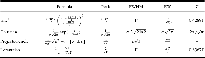
Note that all formulas are normalised to unit area under the profile.
3 A CONSISTENT RESOLUTION CRITERION
This paper aims to present criteria by which resolving power can be more meaningfully compared across LSFs of different functional forms. Two approaches have been taken. In Section 5, a criterion based on wavelength accuracy will be given. However, the first criterion, to be discussed in this section, is developed by recognising that what an astronomer means by two close spectral lines being resolved is that the two can be seen separately and can have their strengths and positions (wavelengths) measured without undue influence of one on the other. There will still be an arbitrary definition of what constitutes ‘undue’ influence, but the aim is to ensure that there is only one arbitrary definition and that all other measures are consistent with it. The influence of one spectral line on another is measured by its effect in increasing the noise in measurement of the flux of the line.
The procedure to use this method was to generate LSFs of various functional forms, with two equal strength peaks at separations varying from 0.8 to 2.0 × FWHM, add noise to them, and then perform least-squares fits to extract the positions and strengths of the two peaks.Footnote 2 Importantly, the width of each peak was treated as known rather than as a further variable to fit. This was done for two reasons: (1) at the ultimate closest resolvable approach of two spectral lines, it is recognised that the issue is to separate two unresolved lines. It is well known that if the line width is itself resolved, then lines would have to be further apart to be properly resolved. This is not what ‘spectral resolving power’ is taken to mean. (2) Once two lines begin to blend, in the presence of noise the fitting process would be likely to result in one broadened line rather than two partly blended lines.
Figure 2 shows an example of two lines, with added noise, and the least-squares fits. The simulations were performed using the same noise power within the FWHM for each LSF form. This is an unavoidably arbitrary choice of noise power normalisation, but it does not influence the results to be derived from these simulations. The different LSFs were normalised to the same total area, i.e. flux (not peak). This reflects the fact that total signal power in the spectral line is the quantity of importance to astronomers. Figure 3 shows the results of this process. For each of the five LSFs shown (sinc2, Gaussian, Lorentzian, projected circle, and projected circle convolved with a Gaussian), a large number of trials (4000) were done at each of 25 separations from 0.8 to 2.0 × FWHM. From each set of 4000 trials, the standard deviation of the least-squares-fitted flux was found. The smooth curves shown are semi-empirical model fits to the data of standard deviation versus peak separation and are used to smooth out irregularities due to random fluctuations. The functional form fitted was
 \begin{equation}
\sigma _{\rm fitted\ flux} = C \ ({\rm autocorrelation}(B^2(x)))^\gamma + \sigma _{\rm flux,iso},
\end{equation}
\begin{equation}
\sigma _{\rm fitted\ flux} = C \ ({\rm autocorrelation}(B^2(x)))^\gamma + \sigma _{\rm flux,iso},
\end{equation}
Example of dual peak fitting. Blue line: two Gaussians each with peak 9.3941 (area 10.0), unity FWHM, at a separation of 1.1× FWHM, with 62.6 samples over an FWHM, and subject to independent Gaussian distributed noise with standard deviation 1.0 in each sample. Red curve: the least-squares fit to two Gaussians. This plot shows one of 4000 realisations at one of 25 peak spacings.

The variation of σflux versus separation of two peaks, for five different LSF forms. From highest to lowest at peak separation = 1.0 the curves are: black, Lorentzian; green, Gaussian; blue, sinc2; magenta, projected circle convolved with a Gaussian (see Section 6); red, projected circle. The blue square on the sinc2 curve indicates the Rayleigh criterion separation.

At large separations, the standard deviations approach the value obtained for an isolated peak, i.e. by this criterion the lines are not influencing each other, and are fully resolved. However, the Lorentz profile has such broad wings that it has not yet reached a constant level at the separation of 2.0 FWHM. The Lorentz profile shows the effect of one peak disturbing another (i.e. increasing its noise) at substantially larger separations than the other LSFs, when measured in multiples of the FWHM.
The sinc2 and Gaussian LSFs show very similar curves in Figure 3, consistent with the fact that both are peaked functions which drop smoothly and rapidly towards zero.
The projected circle LSF has a very different curve of σflux versus separation. There is no effect at all of one peak on the other until they begin to touch, at $2/\sqrt{3} \times$
FWHM = 1.1547 × FWHM. At smaller separations, there is some interaction but it is very small because the profiles are convex with such steep sides. Figure 3 also includes a curve for a projected circle LSF convolved with a Gaussian of width such that the final FWHM is a minimum (see Section 6).
$2/\sqrt{3} \times$
FWHM = 1.1547 × FWHM. At smaller separations, there is some interaction but it is very small because the profiles are convex with such steep sides. Figure 3 also includes a curve for a projected circle LSF convolved with a Gaussian of width such that the final FWHM is a minimum (see Section 6).
Figure 3 makes it clear that different LSF functional forms do indeed have very different properties as regards the mutual effects of two lines, and to simply use the FWHM as a resolution criterion is a poor indicator of spectral resolution as it affects line finding and fitting. It is also clear that the Lorentzian profile will give poor resolution at a given separation in FWHMs, while the projected circle is exceptionally good.
The data in Figure 3 can be used to derive scaling factors to quantitatively compare different LSFs. The method used here was to take a sinc2 profile separated according to the Rayleigh criterion as the standard of ‘just-resolved’ spectral lines. This leads to a σflux value increased by a factor of 1.0514 compared with its limiting value at large separations (i.e. for isolated peaks). Other LSF forms will thus be considered to be just resolved when their σflux values are likewise increased by 1.0514× over the value at large separations. Defining a resolving power according to this criterion:
 \begin{equation}
R_{\sigma {\rm flux}} = R_{\sigma _{\rm flux}=1.0514\times \sigma _{\rm flux,iso}} = R_{\rm FWHM}/ \alpha ,
\end{equation}
\begin{equation}
R_{\sigma {\rm flux}} = R_{\sigma _{\rm flux}=1.0514\times \sigma _{\rm flux,iso}} = R_{\rm FWHM}/ \alpha ,
\end{equation}
Resolution element scaling factors.
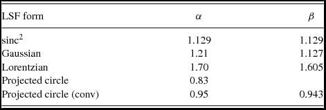
Although the sinc2 profile was used as the standard for resolution, its value of α is not unity because the Rayleigh criterion corresponds to a peak separation of 1.129 × FWHM. The α values show how much the resolving powers determined by the present criterion of equal disturbance in peak fitting due to an adjacent line differ from those based simply on the FWHM. As expected, the Lorentzian is the worst, with an R σflux only 59% of its R FWHM while the projected circle is the best, with R σflux exceeding R FWHM by 20%. The convolved projected circle is a more realistic case (to be discussed in Section 6) and its resolving power, while less than the exact projected circle, is still substantially greater than a Gaussian or sinc2. Figure 4 shows profiles presented in the same style as Figure 1 but with row 2 showing various LSF types with two peaks separated according to the criterion σflux = 1.0514×σflux,iso. These show the separations which are regarded as ‘just resolved’ according to the criterion introduced here.
Five LSF functional forms (top row). The convolved projected circle is the configuration with minimum final FWHM (FWHMprojectedcircle = 1.0532, FWHMGaussian = 0.3432, FWHMfinal = 1.000). The first row shows the single LSFs, while the second row shows a pair of peaks of the corresponding LSF separated according to the criterion σflux = 1.0514×σflux,iso introduced in Section 3. The three numerical values at the right-hand side of each panel are as for Figure 1.

4 LINE PARAMETER UNCERTAINTIES
Before introducing a second method of quantifying resolving power, it is necessary to review the formulas for uncertainties in the flux and position (wavelength) of a single spectral line peak.
When the width of the peak is known and only the amplitude (flux) and position (wavelength) are fitted by least squares, and assuming a symmetrical LSF form, Clarke et al. (Reference Clarke, Frater, Large, Munro and Murdoch1969) give the formulas:
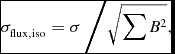 \begin{equation}
\sigma _{\rm flux,iso} = \sigma \left/ \sqrt{\sum {B^2}},\right.
\end{equation}
\begin{equation}
\sigma _{\rm flux,iso} = \sigma \left/ \sqrt{\sum {B^2}},\right.
\end{equation}
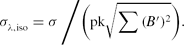 \begin{equation}
\sigma _{\lambda ,{\rm iso}} = \sigma \left/ \Big ( {\rm pk} \sqrt{\sum {(B^{\prime })^2}}\Big ).\right.
\end{equation}
\begin{equation}
\sigma _{\lambda ,{\rm iso}} = \sigma \left/ \Big ( {\rm pk} \sqrt{\sum {(B^{\prime })^2}}\Big ).\right.
\end{equation}
In these formulas, σ is the rms noise in each wavelength channel and is assumed to be the same for all channels. The summation is over all wavelength channels contributing to the profile. The LSF function is B, and B′ denotes its derivative with respect to wavelength. Note that in these equations B is normalised to a peak of 1.00, and the ‘pk’ in equation (4) is the peak flux of the response whose σλ is to be found. These formulas have been verified by Monte Carlo tests and show that the precision in finding the strength of a peak depends most on the values where the intensity is greatest, while the precision in the location of the peak depends on the regions of greatest slope.
It is not appropriate in this paper to consider a detailed noise model where one would take into account shot noise from both the object and the background sky, as well as read-out noise and dark noise. Instead, it will be suffice to use the above assumption of constant noise in all channels. The results are thus most directly applicable to spectra that are background (or read-out noise) limited but serve as a guide for other noise models as well. They can also be applied to absorption lines, especially those that do not depress the continuum by a large fraction.
In the present work, a large number of channels (pixels) have been used, e.g. 62.5 or 100 across the FWHM, to avoid the issue of sampling effects. However, for the projected circle, the gradient B′ becomes infinite as the intensity drops to zero, and the sum in equation (4) would always be dominated by the edge pixels (see Section 6). Hence, this case is omitted here. The more realistic convolved projected circle avoids this problem.
5 A SECOND RESOLUTION CRITERION
The second method to be considered originates from a somewhat independent property of high resolving power, namely the ability to measure accurate positions (wavelengths) of unresolved spectral lines. Thus, two spectrographs can be considered as having equal resolving power if they give the same wavelength accuracy despite their different LSF forms, assuming that the noise power per wavelength interval remains constant and equal total fluxes are received in both cases.
To compare resolving powers using this criterion, there is no need to perform noise simulations as in Section 3 but instead equation (4) can be used as follows.
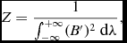
Define
 \begin{equation}
Z = \frac{1}{\int _{-\infty }^{+\infty }(B^{\prime })^2\ \text{d} \lambda },
\end{equation}
\begin{equation}
Z = \frac{1}{\int _{-\infty }^{+\infty }(B^{\prime })^2\ \text{d} \lambda },
\end{equation}
 \begin{equation}
Z \simeq \frac{1}{\Delta \lambda \sum {(B^{\prime })^2}},
\end{equation}
\begin{equation}
Z \simeq \frac{1}{\Delta \lambda \sum {(B^{\prime })^2}},
\end{equation}
Equation (4) can now be written as
 \begin{equation}
\sigma _\lambda = \sigma Z^{\frac{1}{2}} \Delta \lambda ^\frac{1}{2} / {\rm pk,}
\end{equation}
\begin{equation}
\sigma _\lambda = \sigma Z^{\frac{1}{2}} \Delta \lambda ^\frac{1}{2} / {\rm pk,}
\end{equation}
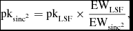
The basis of this second resolution criterion is that σλ,LSF of any LSF will be equated to σλ, sinc2 , with the condition that the two profiles have equal total fluxes (not equal peak values).
The condition for equal total fluxes is simply
 \begin{equation}
{\rm pk}_{{\rm sinc}^2} = {\rm pk}_{\rm LSF} \times \frac{{\rm EW}_{\rm LSF}}{{\rm EW}_{{\rm sinc}^2}},
\end{equation}
\begin{equation}
{\rm pk}_{{\rm sinc}^2} = {\rm pk}_{\rm LSF} \times \frac{{\rm EW}_{\rm LSF}}{{\rm EW}_{{\rm sinc}^2}},
\end{equation} $\text{EW}$
denotes the equivalent width. Equating the σλ values for the given LSF and sinc2 and using the values of Z and
$\text{EW}$
denotes the equivalent width. Equating the σλ values for the given LSF and sinc2 and using the values of Z and $\text{EW}$
for sinc2 from Table 1, there follows
$\text{EW}$
for sinc2 from Table 1, there follows
 \begin{equation}
{\rm FWHM}_{{\rm sinc}^2} = 1.2231 Z_{\rm LSF}^{\frac{1}{3}} {\rm EW}_{\rm LSF}^{\frac{2}{3}}.
\end{equation}
\begin{equation}
{\rm FWHM}_{{\rm sinc}^2} = 1.2231 Z_{\rm LSF}^{\frac{1}{3}} {\rm EW}_{\rm LSF}^{\frac{2}{3}}.
\end{equation}
This is the FWHM of a sinc2 profile which would have the same wavelength noise error as the actual LSF being examined. If the value is large, it means that a wide sinc2 could give accuracy equal to the LSF, i.e. the LSF is poor (e.g. a Lorentzian). If the FWHMsinc2 is narrow, it means that a high-resolution sinc2 is needed to equal the accuracy of a good LSF, e.g. the convolved projected circle.
The final step is to form the ratio of this calculated FWHMsinc2 with that of the actual LSF and scale it by a factor 1.129, which will make the final scaled resolving powers consistent with the Rayleigh criterion for sinc2 profiles. This gives
 \begin{equation}
\beta = 1.3809 \ Z_{\rm LSF}^{\frac{1}{3}} {\rm EW}_{\rm LSF}^{\frac{2}{3}}/ {\rm FWHM}_{\rm LSF}.
\end{equation}
\begin{equation}
\beta = 1.3809 \ Z_{\rm LSF}^{\frac{1}{3}} {\rm EW}_{\rm LSF}^{\frac{2}{3}}/ {\rm FWHM}_{\rm LSF}.
\end{equation}
Values of β for the standard LSF forms are included in Table 2, except for the projected circle where the infinite gradient limit makes the calculation invalid. Values are quite similar to the α scaling factors derived in Section 3.
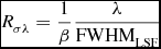
The interpretation of β is that
 \begin{equation}
\delta \lambda _{\sigma \lambda } = \beta \ {\rm FWHM}_{\rm LSF}
\end{equation}
\begin{equation}
\delta \lambda _{\sigma \lambda } = \beta \ {\rm FWHM}_{\rm LSF}
\end{equation}
 \begin{equation}
R_{\sigma \lambda } = \frac{1}{\beta } \frac{\lambda }{{\rm FWHM}_{\rm LSF}}
\end{equation}
\begin{equation}
R_{\sigma \lambda } = \frac{1}{\beta } \frac{\lambda }{{\rm FWHM}_{\rm LSF}}
\end{equation}
This criterion will be easier to use in practice than the σflux-based criterion of Section 3. For an empirically determined LSF, for example resulting from ray tracing of a spectrograph design, one would need to interpolate the LSF to a fine sampling interval, and smooth out any fine structure artefacts from the LSF calculation (e.g. from a finite number of traced rays), then use equation (6) to find the noise width and also find the FWHM and equivalent width (area/peak). Then, equation (10) can be used to find the scaling factor, which is finally applied in equation (12). In the case of an asymmetric LSF, the more general form of equation (4) given by Clarke et al. (Reference Clarke, Frater, Large, Munro and Murdoch1969, equation (A7))Footnote 3 should be used, although the corrections for asymmetry are small.
6 PROJECTED CIRCLE LSF
The projected circle LSF is important in practice and has very different properties compared with other forms, and so warrants further discussion. The use of multi-mode fibres to feed images to a pseudo-slit in a spectrograph is increasingly common. Taking the fibre exit face as a uniformly illuminated circle (a good approximation given the spatial scrambling produced by transmission along the fibre), when its image has been integrated over the spectrograph’s spatial direction, the result will be the projected circle as illustrated in panel 1D of Figure 1. It differs markedly from the sinc2, Gaussian, and Lorentzian forms in that the projected circle LSF approaches the x-axis with infinite slope. This convex-outward form results in the formation of a central spike when two such LSFs overlap, as in Figure 1.
Interestingly, the projected circle line profile also results from Doppler broadening of an intrinsically narrow line in a rapidly rotating star. This is because the radial velocity is constant along strips parallel to the rotation axis, and the flux at any one wavelength is due to an integration along such a strip, i.e. a projection. The effects of the very steep sides of such a profile have been noted, and Dravins (Reference Dravins1992) drew attention to the sharp spectral features that could appear at wavelengths where no spectral line is present, i.e. the central spikes as seen in Figure 1. He also noted that information about the true stellar spectrum could be obtained regarding features considerably narrower than the FWHM of the full broadened profile—this is again due to the steep sides, which lead to the central spike being narrow and easily smoothed out (in this case, by intrinsic line width in a stellar spectrum).
As shown in Section 3, the lack of wings of the projected circle LSF results in minimal noise interaction of two close lines, i.e. its effective resolving power is substantially higher than its FWHM would suggest.
The pure projected circle LSF cannot be directly compared with other LSFs as regards wavelength uncertainties, because of the infinite slopes. This means that however fine the sampling may be, the β value will still depend on the sampling interval. This is illustrated in Figure 5, which shows β dropping approximately logarithmically with increasing sampling frequency. The values of β shown are all substantially less than any of those in Table 2. Even with some blurring due to aberrations, a well-sampled LSF resembling the projected circle will have much higher wavelength accuracy than a Gaussian-like peak of the same FWHM.
Variation of β for a projected circle LSF as a function of the number of samples across the full-width to zero intensity.

One of the peculiarities produced by the convex boxy shape of this LSF is that the FWHM is reduced by convolution with a Gaussian of moderate width. This effect was noted in the design of the AAOmega spectrograph (Saunders Reference Saunders2005). This is another illustration of the inadequacy of FWHM as a measure of resolution, since one would not claim that the convolution of the LSF by spectrograph aberrations increases the resolving power. Figure 6 illustrates this behaviour, using a projected circle LSF of FWHM = 1.00 convolved with Gaussians of various FWHMs up to 0.7. The resulting FWHM drops by as much as 5%, when the Gaussian FWHM = 0.3259, before rising again as the Gaussian convolving function is further broadened. Figure 7 shows three of the profiles: the pure projected circle, the case of the minimum final FWHM, and the case of Gaussian FWHM = 0.595, which restores the final FWHM to 1.00, albeit with a very different LSF form compared with the initial projected circle. The case of the minimum final FWHM was used as the example of a convolved projected circle in Table 2 and Figures 3 and 4.
Final FWHM after convolving a projected circle LSF of unity FWHM with a Gaussian of FWHM as given by the horizontal axis.

Three of the resulting curves from the convolutions of Figure 6. The curves from highest to lowest at the peak are: black, pure unconvolved projected circle; blue, Gaussian FWHM = 0.3259 gives the minimum final FWHM of 0.9494; red, Gaussian FWHM = 0.595 results in a final FWHM of 1.00.

7 CONCLUSIONS
The analysis above has shown that characterising the resolution δλ of a spectrograph by its instrumental FWHM is a poor measure because it fails to take fully into account the variation among different LSF forms of the quantities which matter most in spectroscopy—namely the disturbance which a spectral line causes to a near neighbour, or the accuracy with which a single line’s wavelength can be measured. Using these two criteria, a very different picture emerges, as shown by the α and β scaling factors in Table 2. There is more than a factor of two difference in resolving power between the best and worst LSFs (with identical FWHM) when resolving power is measured on a consistent scale.
Comparing the various resolution criteria shown in Figure 1 with the σflux-based criterion of Figure 4 shows that the equivalent width is the one that comes closest to matching the consistent resolution scale introduced here. However, the match is not exact, with a significant difference in the case of the Gaussian LSF.
The Lorentzian LSF’s broad wings greatly increase its effective δλ and hence reduce the resolving power of an instrument with this LSF well below the value given by the FWHM. It is well known by users of imaging Fabry–Perot instruments, for example, that this LSF makes the instrument unsuitable for absorption line studies, because a line’s core is influenced by convolution with continuum fluctuations over a substantial wavelength range. Here, this influence has been quantified and the Lorentzian’s low relative resolving power explicitly demonstrated.
Conversely, the projected circle, even after smoothing by significant aberrations, has a steep-sided form which gives substantially higher resolving power than its FWHM would suggest. Gaussian and sinc2 profiles have properties intermediate between these two extremes. However, even they have ambiguities at the 10%–15% level, with a pair of Gaussian profiles requiring a separation of 1.129 × FWHM to achieve the 81% relative minimum of a generalised Rayleigh criterion. Either of the two resolution element scaling factors can serve as a quality indicator for any given LSF profile.
It is notable that the α and β scaling factors in Table 2 are quite similar for a given LSF type, despite the former being based on the additional error in fitting the flux of a line caused by a near neighbour, while the latter is based on the accuracy of wavelength determination for isolated lines. This agreement strengthens the case for using one of these resulting scaling factors to bring resolving power of any spectrograph on to a consistent scale. In principle, the ‘α’ factor, based on mutual disturbance in fitting a line, is the more appropriate in low-to-moderate signal/noise spectra, while the ‘β’ factor, based on wavelength accuracy, is the more appropriate for high-resolution, high signal/noise work. However, given the similarity of the two factors and that the β factor is much easier to calculate for a general empirically determined instrumental profile, the β factor is recommended as a suitable standard measure for comparison of resolving power between different spectrographs.



