

1 INTRODUCTION
The mechanical properties of glacier beds, hereafter called basal mechanics, are a fundamental component of glacier dynamics. The importance of basal mechanics is most pronounced in areas of fast-flowing ice, where much of the ice flow is likely to be accommodated by slip along or deformation within the bed and where resistive basal shear traction can be appreciably less than gravitational driving stress (e.g. Raymond, Reference Raymond1996; Tulaczyk and others, Reference Tulaczyk, Kamb and Engelhardt2000b; Morlighem and others, Reference Morlighem, Seroussi, Larour and Rignot2013). The mechanical properties of glacier beds are not fully understood, and this has clear implications for the veracity of models of future glacier states (Schoof, Reference Schoof2007a; Favier and others, Reference Favier2014; Joughin and others, Reference Joughin, Smith and Medley2014: Tsai and others, Reference Tsai, Stewart and Thompson2015). We can improve upon our understanding of basal mechanics by studying temporal variabilities in basal slip, leveraging the response of glaciers to changes in environmental forcing to constrain the set of admissible models of basal mechanics. Here we focus on the special case of the response of land-terminating glaciers with deformable beds to surface meltwater flux.
Glaciers accelerate and decelerate on hourly-to-seasonal timescales in response to surface meltwater flux, changes in terminus position and thinning at the margins (e.g. Iken and Bindschadler, Reference Iken and Bindschadler1986; Sugiyama and Gudmundsson, Reference Sugiyama and Gudmundsson2004; Rignot and Kanagaratnam, Reference Rignot and Kanagaratnam2006; Joughin and others, Reference Joughin2008; Bartholomew and others, Reference Bartholomew2010). The latter two perturbations primarily affect marine- and lacustrine-terminating glaciers and are not given further consideration in this study. Because viscous deformation rates are controlled by the geometry and mechanical properties of ice, which remain approximately constant on sub-annual timescales, changes in basal mechanical properties are the only plausible sources of observed hourly to seasonal timescale flow variability in land-terminating glaciers. These short-timescale ice flow variations have been shown to correlate with surface meltwater flux in the early melt season, sometimes becoming increasingly muted as the melt season progresses and the basal hydrological system evolves (Sugiyama and Gudmundsson, Reference Sugiyama and Gudmundsson2004; Bartholomew and others, Reference Bartholomew2010; Pimentel and Flowers, Reference Pimentel and Flowers2011; Moon and others, Reference Moon2014).
The states of basal hydrological systems are thought to be bounded by two configurations: (1) cavities that open downstream of bumps and (2) channels that are melted into the base of the ice by flowing water (Röthlisberger, Reference Röthlisberger1972; Nye, Reference Nye1976; Kamb, Reference Kamb1987; Schoof, Reference Schoof2010). Beginning in spring, water that drains to a glacier's bed likely inundates an inefficient distributed hydrological system, effectively lubricating the bed and accelerating glacier flow (Lliboutry, Reference Lliboutry1968; Kamb, Reference Kamb1987; Raymond and others, Reference Raymond, Benedict, Harrison, Echelmeyer and Sturm1995). As the melt season progresses, linked cavities eventually form efficient, arterial channel networks if sufficient water flux is available (Schoof, Reference Schoof2010; Sundal and others, Reference Sundal2011). Under steady state conditions, channel networks feature lower water pressure than distributed systems and, consequently, lower glacier speeds (Pimentel and Flowers, Reference Pimentel and Flowers2011; Hewitt, Reference Hewitt2013; Werder and others, Reference Werder, Hewitt, Schoof and Flowers2013). Throughout the melt season and regardless of the hydrological state, enhanced water flux from rainfall or elevated melt rates can temporarily overwhelm and pressurize basal hydrological systems leading to evanescent increases in glacier flow (Shepherd and others, Reference Shepherd2009; Bartholomew and others, Reference Bartholomew2010; Schoof, Reference Schoof2010). Increasing the frequency and duration of these accelerations results in dynamic glacier thinning (Parizek and Alley, Reference Parizek and Alley2004).
Evolution of the basal hydrological system complicates the response of glacier flow to surface meltwater flux, leading some authors to suggest that increased meltwater flux can enhance dynamic mass loss in a warming climate (e.g. Zwally and others, Reference Zwally2002; Parizek and Alley, Reference Parizek and Alley2004; Bougamont and others, Reference Bougamont2014) while others postulate a limited response (e.g. Joughin and others, Reference Joughin2008; Tedstone and others, Reference Tedstone2013, Reference Tedstone2015). Understanding the dynamic response of glaciers to surface meltwater flux and the potential for dynamically enhanced mass loss in warming climates requires understanding of two separate questions: How does basal water pressure respond to surface meltwater flux and how does glacier flow respond to changes in basal water pressure? In this study, we address only the latter question while considering surface meltwater flux to be the driver of basal water pressure variations.
To better understand the fundamental mechanics of glacier beds and the response of glacier flow to surface meltwater flux, we consider Hofsjökull, a relatively small ice cap in central Iceland (Fig. 1). Hofsjökull experiences seasonal melt and contains multiple land-terminating outlet glaciers. Land-termination isolates the influence of basal water pressure on glacier flow by eliminating ocean tidal forcing and seasonal accelerations attributable to displacement of calving fronts (Joughin and others, Reference Joughin2008). Hofsjökull's small size (diameter ~40 km), gentle surface slopes and dome-like shape (Fig. 1b) allow all outlet glaciers to experience roughly the same climate, thereby helping to elucidate the spatially heterogeneous response of individual outlet glaciers to comparable environmental forcing. Hofsjökull, which blankets a dormant volcanic caldera, is known to be underlain by till (Björnsson and others, Reference Björnsson, Pálsson, Sigurðsson and Flowers2003; Björnsson and Pálsson, Reference Björnsson and Pálsson2008), which we show deforms plastically. While observations indicate that plastically deforming beds are well-represented in nature (Boulton, Reference Boulton1979; Iverson and others, Reference Iverson, Hooyer and Baker1998; Tulaczyk and others, Reference Tulaczyk, Kamb and Engelhardt2000a), most models of basal mechanics and the influence of basal water pressure on ice flow dynamics focus on rigid-bedded glaciers. Therefore, while our observations focus solely on Hofsjökull, our physical model and conclusions have implications for understanding glacier systems worldwide.
(a) Shaded relief map of Iceland. Glaciers are white, Hofsjökull is enclosed by the red box and darkened regions delineate volcanic zones. The red triangle shows the location where meteorological data shown in Figure 3 were collected and the blue triangle indicates the study area of Boulton (Reference Boulton1979). (b) Surface topography (Jóhannesson and others, Reference Jóhannesson2013) (colormap and blue contours), ice divides (black lines; modified from Björnsson (Reference Björnsson1986)) and major outlet glaciers of Hofsjökull (Björnsson, Reference Björnsson1988). Contours indicate ice surface elevation in 150 m increments with the maximum contour at 1650 m. Glacier labels stand for: Illviðrajökull (HI), Þjórsárjökull (HÞ), Múlajökull (HM), Blautukvislarjökull (HT), Blágnípujökull (HB), Kvíslajökull (HK) and Sátujökull (HS). Bold labels indicate known surge-type glaciers (Björnsson and others, Reference Björnsson, Pálsson, Sigurðsson and Flowers2003; Minchew and others, Reference Minchew, Simons, Hensley, Björnsson and Pálsson2015). (c) Basal topography relative to mean sea level (Björnsson, Reference Björnsson1986) (colormap and dark contours); dark contours are at 100 m increments. (d) Ice thickness (colormap and dark contours); dark contours are at 100 m increments. (e) Gravitational driving stress τ d = ρghα (colormap and dark contours) with ρ = 9000 kg m−3; dark contours are at 25 kPa increments. In (c)–(e), light contour lines are the same as in (b)

2 DATA AND METHODS
2.1 Surface velocity observations
We capture temporal flow variability in multiple outlet glaciers during the early melt season by inferring complete velocity fields over Hofsjökull using repeat-pass interferometric synthetic aperture radar (InSAR) data (Fig. 2). Airborne InSAR data were collected with NASA's Uninhabited Aerial Vehicle Synthetic Aperture Radar (UAVSAR) (Hensley and others, Reference Hensley2009) in June 2012, beginning ~2 weeks after the onset of seasonal melt on Hofsjökull (Fig. 3), and in February 2014, the middle of winter (Minchew and others, Reference Minchew, Simons, Hensley, Björnsson and Pálsson2015). We expect basal water pressure during winter to be at or near annual minimum pressure due to the lack of surface melt, so we take the February data as the reference velocity field (Fig. 2a). Because InSAR measures the component of displacement occurring in the time between two radar acquisitions along the (oblique) radar line-of-sight (LOS) vector (Rosen and others, Reference Rosen2000), we designed the UAVSAR data collection to observe all of Hofsjökull from at least three unique LOS directions with approximately equal azimuthal spacing. For each azimuth heading, three flight tracks were needed to cover all of the ice cap, yielding a total of nine different flight tracks (Minchew and others, Reference Minchew, Simons, Hensley, Björnsson and Pálsson2015). UAVSAR was flown aboard a NASA Gulfstream III aircraft that cruises at ~12.5 km altitude, providing an incidence angle range of 22°–65°. We incorporated all InSAR data collected on given dates to estimate the horizontal velocity fields using a Bayesian approach (Minchew and others, Reference Minchew, Simons, Hensley, Björnsson and Pálsson2015). The resulting velocity fields have ~200 m resolution with typical errors <1 cm d−1 (Figs 2g–i).
Seasonal ice flow variability. (a) Horizontal surface speeds on Hofsjökull recorded 1–3 February 2014. Black contours indicate ice surface elevation in 150 m increments (maximum contour at 1650 m). (b) and (c) Horizontal surface speed relative to (a) recorded 3–4 June 2012 and 13–14 June 2012, respectively. (d) Horizontal surface speed on 13–14 June 2012 relative to 3–4 June 2012. (e) and (f) Transects of horizontal surface speed along A-A’ and B-B’, respectively. (g)–(i) Formal errors in InSAR-derived estimates of the horizontal velocity fields, derived from the method in Minchew and others (Reference Minchew, Simons, Hensley, Björnsson and Pálsson2015), for data collected (g) 1–3 February 2014, (h) 3–4 June 2012 and (i) 13–14 June 2012. Ice divides and labels in (b) are the same as in Figure 1b.

(a) Cumulative seasonal melt inferred from meteorological data collected at ~1100 m elevation on nearby Langjökull glacier (red triangle in Fig. 1). Data include incoming and outgoing solar and thermal radiation, relative humidity and windspeed and temperature at ~3 m above the ice surface. (b) Ambient temperature is from the same meteorological data. Red dashed lines indicate the times when UAVSAR data were collected.

2.2 Basal mechanics
To infer the basal shear traction and slip rate, we use the observed velocity fields to constrain finite-element ice flow models. Employing the Ice Sheet Systems Model (ISSM) (Morlighem and others, Reference Morlighem2010), we constructed the geometry of Hofsjökull using basal topography derived from ice-penetrating radar surveys (Björnsson, Reference Björnsson1986) and lidar-derived surface topography (Jóhannesson and others, Reference Jóhannesson2013) (Figs 1b–e). In ISSM the basal boundary condition uses a Weertman-type sliding law whose scalar form is defined as:
 $${\tau _{\rm b}} = Cu_{\rm b}^{1/{\rm m}}$$
where τ
b is the basal shear traction, u
b is the basal slip rate, m ≥ 1, and coupling between ice and the bed is indicated by the non-negative scalar C (e.g. Weertman, Reference Weertman1957; Gudmundsson and Raymond, Reference Gudmundsson and Raymond2008). Using a higher-order ice flow model to estimate viscous deformation in the ice (Blatter, Reference Blatter1995; Pattyn, Reference Pattyn2003; Morlighem and others, Reference Morlighem, Seroussi, Larour and Rignot2013), we solved for the optimal values of C at each mesh node such that τ
b satisfies global stress balance and u
b minimizes the residual between modeled and observed surface velocities. Ice is treated as an incompressible viscous fluid whose constitutive relation is ${\tau _{ij}} = 2\eta {\dot \varepsilon _{ij}}$
, where
${\tau _{ij}} = 2\eta {\dot \varepsilon _{ij}}$
, where ${\dot \varepsilon _{ij}}$
and τ
ij
are components of the strain rate and deviatoric stress tensors, respectively,
${\dot \varepsilon _{ij}}$
and τ
ij
are components of the strain rate and deviatoric stress tensors, respectively, $\eta = {A^{ - 1/n}}\dot \varepsilon _{\rm e}^{\left( {1 - n} \right)/n} /2$
is the effective dynamic viscosity, and
$\eta = {A^{ - 1/n}}\dot \varepsilon _{\rm e}^{\left( {1 - n} \right)/n} /2$
is the effective dynamic viscosity, and ${\dot \varepsilon _{\rm e}}$
is effective strain rate (calculated from the second invariant of the strain rate tensor). Hofsjökull is temperate and damage in the ice is predominantly restricted to areas that are not of interest in this study (Björnsson and others, Reference Björnsson, Pálsson, Sigurðsson and Flowers2003), so we take A and n to be spatially and temporally constant, assigning n = 3 and A = 2.4 × 10⁻²⁴ Pa−3 s−1 (Cuffey and Paterson, Reference Cuffey and Paterson2010). Results given in this study were obtained using m = 5. Further details of the inversion and ice flow model are given by Morlighem and others (Reference Morlighem, Seroussi, Larour and Rignot2013).
${\dot \varepsilon _{\rm e}}$
is effective strain rate (calculated from the second invariant of the strain rate tensor). Hofsjökull is temperate and damage in the ice is predominantly restricted to areas that are not of interest in this study (Björnsson and others, Reference Björnsson, Pálsson, Sigurðsson and Flowers2003), so we take A and n to be spatially and temporally constant, assigning n = 3 and A = 2.4 × 10⁻²⁴ Pa−3 s−1 (Cuffey and Paterson, Reference Cuffey and Paterson2010). Results given in this study were obtained using m = 5. Further details of the inversion and ice flow model are given by Morlighem and others (Reference Morlighem, Seroussi, Larour and Rignot2013).
A Weertman-type sliding law (Eqn (1)) with small values of m may not be physically applicable to Hofsjökull because of its till-covered bed (Iverson and others, Reference Iverson, Hooyer and Baker1998; Björnsson and others, Reference Björnsson, Pálsson, Sigurðsson and Flowers2003; Björnsson and Pálsson, Reference Björnsson and Pálsson2008). The exponent 1/m is a prescribed value in ISSM so it is important that we test the sensitivity of inferred basal shear traction and basal slip rate to m. We expect inferred basal shear traction to be insensitive to prescribed values of m because basal shear traction must satisfy global stress balance (Joughin and others, Reference Joughin, MacAyeal and Tulaczyk2004). To confirm this postulate, we infer C using multiple values of m, such that 1 ≤ m ≤ 50. The higher-order ice flow model is computationally expensive to implement so we only inferred basal conditions with the higher-order model for m = 1, 3 and 5. For m = 1, 3, 5, 10, 20 and 50 we applied the 2-D shallow-shelf model (e.g. MacAyeal, Reference MacAyeal1989) to infer basal conditions using ISSM and the same mesh grids. The higher-order and shallow-shelf models yield the same basal shear traction for m = 1, 3 and 5, so we expect results from the shallow-shelf model and large m values to represent the sensitivity of inferred τ
b to large m. For all tested m values, we retrieve basal shear traction fields that are within a few percent of one another because $C \propto u_{\rm b}^{ - 1/m} $
for any m in all observed data (Fig. 4). We will exploit this behavior to interpret inferred basal shear tractions in the context of sliding laws that differ from Eqn (1).
$C \propto u_{\rm b}^{ - 1/m} $
for any m in all observed data (Fig. 4). We will exploit this behavior to interpret inferred basal shear tractions in the context of sliding laws that differ from Eqn (1).
(a)–(c) Basal slipperiness versus basal slip rate inferred using a linear viscous sliding law (m = 1 in Eqn (1)) for horizontal surface speeds recorded (a) 1–3 February 2014, (b) 3–4 June 2012 and (c) 13–14 June 2012. Blue lines are the best-fit linear trends. (d) Basal slipperiness versus basal slip rate for 13–14 June inferred with m = 1, 3 and 5 (Eqn (1)). The solid black line is the best linear fit and indicates that, in general, $C \propto u_{\rm b}^{ - 1/m} $
for any m, implying that τ
b is independent of u
b and the bed deforms plastically.
$C \propto u_{\rm b}^{ - 1/m} $
for any m, implying that τ
b is independent of u
b and the bed deforms plastically.

3 RESULTS
3.1. Surface velocity observations
Comparing winter and summer surface speeds, we find that early summer acceleration is evident in most outlet glaciers (Figs 2a–f). The only named glacier in our dataset that does not appear to accelerate is Kvíslajökull (Fig. 1b), which partially drains ice collected in the central caldera through a notch in the caldera rim, causing the observed surface speeds to be dominated by viscous deformation (Minchew and others, Reference Minchew, Simons, Hensley, Björnsson and Pálsson2015). In other glaciers, typical increases in velocity are approximately double wintertime velocities, meaning that faster flowing areas tend to experience higher acceleration than slower moving areas. Highest accelerations are more evident at intermediate elevations (Figs 2e and f), with ice flow in higher- and lower-elevations indicating lower rates of acceleration, likely due to limited surface meltwater supply and the existence of a relatively efficient basal hydrological system, respectively. These observations are consistent with an influx of surface meltwater to, and subsequent pressurization of, a distributed hydrological system along much of the length of the outlet glaciers during the early melt season.
Between 3–4 June and 13–14 June the meteorological data indicate 4 days of little-to-no melt followed by 6 days of higher melt rates (Fig. 3) and UAVSAR data show notable changes in the relative surface velocities of the outlet glaciers. Glaciers that previously accelerated slowed except Sátujökull (transect A-A’; Fig. 2a) and Illviðrajökull, suggesting that during the 10-day interim the capacity of the hydrological system beneath the other glaciers increased through a combination of enhanced efficiency, connectivity and the opening of cavities leeward of bumps in the bed (Figs 2b and 2c) (e.g. Schoof, Reference Schoof2010; Hoffman and Price, Reference Hoffman and Price2014; Andrews and others, Reference Andrews2014). While they likely have similar bed properties to the rest of Hofsjökull (Björnsson and others, Reference Björnsson, Pálsson, Sigurðsson and Flowers2003), Sátujökull and Illviðrajökull have relatively small water catchment areas feeding their hydrological systems (Björnsson, Reference Björnsson1988), which can delay evolution of the subglacial hydrological system (Schoof, Reference Schoof2010). Glaciers in the southwest quadrant slowed to near wintertime velocities, while other outlet glaciers only partially slowed, consistent with differential evolution of the basal hydrological systems (Iken and Bindschadler, Reference Iken and Bindschadler1986; Sugiyama and Gudmundsson, Reference Sugiyama and Gudmundsson2004; Bartholomew and others, Reference Bartholomew2010). Múlajökull (transect B-B’; Fig. 2a) slowed considerably, losing approximately half of its early melt season acceleration, but maintained elevated flow speeds. Þjórsárjökull generally experienced slowdown between 3–4 June and 13–14 June, though its southern-most portion accelerated slightly over the same time. There are no indications that any outlet glaciers slowed to below wintertime flow rates except in upstream areas with slightly reduced flow rates located at elevations that experienced little or no surface melt (Fig. 3). Given their overall minor changes and general association with relatively strong beds (next section), we do not consider areas that experience higher wintertime ice speeds to be germane to this study.
3.2 Basal mechanics
Modeled surface speeds match observed surface speeds to within 10% (20%) over more than 50% (70%) of areas where observed flow speeds exceed 4 cm d−1 (Fig. 5). Notable misfits include the midstream region of Múlajökull, lower extent of Blöndujökull, and high-velocity region of Kvíslajökull (all in green dashed circle and respectively labeled A, B and C; Fig. 5a). In all three cases the modeled viscous flow component of surface speed exceeds the observed surface flow speed. Three likely causes for the misfits in these areas are: (1) ice thickness overestimation, (2) excessive surface slope estimates and (3) failure of the underlying assumptions in the higher-order ice flow model. Viscous flow in areas with low basal slip rates approximately scales as α n h n+1, where α is the surface slope (radians) and h is ice thickness, so small errors in ice thickness and surface slope are amplified in the viscous flow estimates. In all three glaciers in question, surface crevassing led to gaps in the bedrock topography observations, which were filled by interpolation (Björnsson, Reference Björnsson1986). Modeling errors on Kvíslajökull could be exacerbated by a large increase in local surface slope that is not properly accounted for in the surface elevation measurements, which were collected at a different time than the InSAR data. The upper extent of Kvíslajökull is coincident with a significant slope break at the lip of the underlying caldera and, therefore, may be especially prone to errors in surface slope. Where high horizontal normal stresses are present, the assumption of hydrostatic normal pressure at the bed breaks down and the use of the higher-order model incurs larger errors (Schoof and Hindmarsh, Reference Schoof and Hindmarsh2010). However, for this study, our interest is in areas with relatively high and seasonally variable basal slip rates, all of which are well fit by the modeled ice flow and have flow characteristics that support the underlying assumptions in the higher-order model (Blatter, Reference Blatter1995; Pattyn, Reference Pattyn2003; Schoof and Hindmarsh, Reference Schoof and Hindmarsh2010). Therefore, we disregard the aforementioned and other areas containing high misfits between modeled and observed ice flow (magenta and cyan colored regions in Fig. 5a) and analyze basal shear traction and basal slip rates in the remaining areas.
(a)-(c) Residual surface velocities between modeled and observed surface speeds $(\Delta {u_{\rm s}} = u_{\rm s}^{mod} - u_{\rm s}^{obs} )$
for (a) 1–3 February 2014, (b) 3–4 June 2012 and (c) 13–14 June 2012. (d)–(f) Same as (a)–(c) but normalized by observed surface speeds. Gray regions indicate areas where observed surface speeds are <4 cm d−1.
$(\Delta {u_{\rm s}} = u_{\rm s}^{mod} - u_{\rm s}^{obs} )$
for (a) 1–3 February 2014, (b) 3–4 June 2012 and (c) 13–14 June 2012. (d)–(f) Same as (a)–(c) but normalized by observed surface speeds. Gray regions indicate areas where observed surface speeds are <4 cm d−1.

Inferred basal shear traction and basal slip rate fields indicate that the bed beneath Hofsjökull deforms plastically. Inferred basal shear tractions typically are between 100 and 150 kPa in areas where basal slip rate is non-zero (Figs 6a–h and 7a–f) and are within a factor of two of the gravitational driving stress, τ
d = ρghα, where ρ is the mean density of ice, g is gravitational acceleration, and α is taken to be small such that sin (α) ≈ α (Figs 7g–i). Basal shear tractions generally increase linearly with basal slip rate for slow basal slip ( ${u_{\rm b}}{\rm \lesssim} 5\,{\rm cm} {{\rm \,d}^{ - 1}}$
) and are independent of basal slip rate and observed surface speed in areas of faster slip, behavior that is consistent with a plastically deforming bed. This conclusion is supported by laboratory tests of plastically deforming subglacial till (Kamb, Reference Kamb1991; Tulaczyk and others, Reference Tulaczyk, Kamb and Engelhardt2000a). The existence of plastically deforming till beneath Hofsjökull is bolstered by direct observations of the bed of nearby Breiðamerkurjökull (blue triangle in Fig. 1a) (Boulton, Reference Boulton1979), the known bed composition of Hofsjökull (Björnsson and others, Reference Björnsson, Pálsson, Sigurðsson and Flowers2003; Björnsson and Pálsson, Reference Björnsson and Pálsson2008) and the presence of an active drumlin field at the Mulajökull (transect B-B’ in Fig. 2a) terminus (Johnson and others, Reference Johnson2010). The existence of an active drumlin field is particularly salient given that drumlins are thought to be primarily depositional, rather than erosional, features that arise due to the behavior of plastically deforming till (Fowler, Reference Fowler2000, Reference Fowler, Balmforth and Provenzale2001; Schoof, Reference Schoof2007b). This suite of observations diminishes the applicability of rigid-bed sliding laws to our study site (e.g. Lliboutry, Reference Lliboutry1968; Fowler, Reference Fowler1987; Schoof, Reference Schoof2005) and supports limiting our focus to models that account for deformation within a finite till layer. Though the thickness of the till remains unknown, as do the mechanisms for maintaining a till layer (Iverson, Reference Iverson2010), we note that till layers only need to be centimeters thick to facilitate plastic deformation. The mechanical properties of till layers depend on pore water pressure (Tulaczyk and others, Reference Tulaczyk, Kamb and Engelhardt2000a), represented herein by mean basal water pressure.
${u_{\rm b}}{\rm \lesssim} 5\,{\rm cm} {{\rm \,d}^{ - 1}}$
) and are independent of basal slip rate and observed surface speed in areas of faster slip, behavior that is consistent with a plastically deforming bed. This conclusion is supported by laboratory tests of plastically deforming subglacial till (Kamb, Reference Kamb1991; Tulaczyk and others, Reference Tulaczyk, Kamb and Engelhardt2000a). The existence of plastically deforming till beneath Hofsjökull is bolstered by direct observations of the bed of nearby Breiðamerkurjökull (blue triangle in Fig. 1a) (Boulton, Reference Boulton1979), the known bed composition of Hofsjökull (Björnsson and others, Reference Björnsson, Pálsson, Sigurðsson and Flowers2003; Björnsson and Pálsson, Reference Björnsson and Pálsson2008) and the presence of an active drumlin field at the Mulajökull (transect B-B’ in Fig. 2a) terminus (Johnson and others, Reference Johnson2010). The existence of an active drumlin field is particularly salient given that drumlins are thought to be primarily depositional, rather than erosional, features that arise due to the behavior of plastically deforming till (Fowler, Reference Fowler2000, Reference Fowler, Balmforth and Provenzale2001; Schoof, Reference Schoof2007b). This suite of observations diminishes the applicability of rigid-bed sliding laws to our study site (e.g. Lliboutry, Reference Lliboutry1968; Fowler, Reference Fowler1987; Schoof, Reference Schoof2005) and supports limiting our focus to models that account for deformation within a finite till layer. Though the thickness of the till remains unknown, as do the mechanisms for maintaining a till layer (Iverson, Reference Iverson2010), we note that till layers only need to be centimeters thick to facilitate plastic deformation. The mechanical properties of till layers depend on pore water pressure (Tulaczyk and others, Reference Tulaczyk, Kamb and Engelhardt2000a), represented herein by mean basal water pressure.
Inferred (a)–(d) basal slip rates, (e)–(h) basal shear tractions, (i)–(l) basal water pressures and (m)–(p) normalized basal water pressure p′w = p w/(ρgh) for ρ = 9000 kg m−3. The left column contains properties inferred from data collected 1–3 February 2014 while the two center columns contain inferred properties for 3–4 June 2012 and 13–14 June 2012, relative to the left column. The right column shows 13–14 June 2012 relative to 3–4 June 2012. Bright areas in (i)–(p) indicate regions where τ b = τ y, allowing for direct estimates of basal water pressure, while water pressures in subdued regions (i.e. areas of lower color intensity that tend to appear gray) are an upper bound on the absolute estimates in (i) and (m) or at least one estimate in the differences in (j)–(l) and (n)–(p). Ice divides and labels in (a) are the same as in Figure 1b.

Mechanical properties of the bed. (a)–(c) Inferred basal shear traction versus inferred basal slip. (d)–(f) Inferred basal shear traction versus observed horizontal surface speed. Blue curves (and shaded regions) represent the viscous deformation rate for 250 m (±100 m) thick ice approximated as ${u_{\rm v}} = 2A\tau _{\rm b}^n h/(n + 1)$
. The range of ice thicknesses corresponds to the mean and standard deviation in rapid-flowing areas. (g)–(i) Ratio of inferred basal shear traction to gravitational driving stress versus inferred basal slip rate. In all figures dot colors represent number of data points within each hexagonal bin. Columns contain properties inferred from data collected 1–3 February 2014 (a, d, g) 3–4 June 2012 (b, e, h), and 13–14 June 2012 (c, f, i).
${u_{\rm v}} = 2A\tau _{\rm b}^n h/(n + 1)$
. The range of ice thicknesses corresponds to the mean and standard deviation in rapid-flowing areas. (g)–(i) Ratio of inferred basal shear traction to gravitational driving stress versus inferred basal slip rate. In all figures dot colors represent number of data points within each hexagonal bin. Columns contain properties inferred from data collected 1–3 February 2014 (a, d, g) 3–4 June 2012 (b, e, h), and 13–14 June 2012 (c, f, i).

Given a plastic bed, it is straightforward to estimate mean basal water pressure using inferred basal shear tractions. We assume that basal slip is facilitated solely by plastic bed deformation (Tulaczyk and others, Reference Tulaczyk, Kamb and Engelhardt2000b), thereby ignoring any linear relationship between basal shear traction and basal slip rate at low basal slip rates (Figs 7a–c). We define the bed yield stress using the Mohr-Coulomb criteria (Iverson and others, Reference Iverson, Hooyer and Baker1998; Kamb, Reference Kamb1991; Tulaczyk and others, Reference Tulaczyk, Kamb and Engelhardt2000a):
 $${\tau _{\rm y}} = (\rho gh - {\,p_{\rm w}}){\,f_{\rm c}}$$
where p w is the mean basal water pressure, f c is the internal friction parameter for till and we have assumed negligible till cohesion (Iverson, Reference Iverson2010). For a plastic bed, τ b = τ y wherever basal slip occurs (u b >0) and τ b <τ y where there is no basal slip (u b = 0). By setting τ b = τ y and taking the unknown f c to be the median of published values (f c = 0.4; Iverson, Reference Iverson2010), we can solve for estimates of water pressure (Figs 6i–p). In areas with little or no basal slip (Fig. 6a), the estimated water pressure is the upper bound (indicated by subdued colors in Figs 6i and 6m).
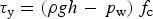
The accuracy of estimated water pressure is relatively insensitive to the chosen value of f c. The error in estimated water pressure arising from incorrect values of f c is given as:
 $$\eqalign{\delta {\,p_{\rm w}} = & \displaystyle{{\partial {\,p_{\rm w}}} \over {\partial {\,f_{\rm c}}}}\delta {\,f_{\rm c}} \cr = & \displaystyle{{{\tau _{\rm y}}} \over {\,f_{\rm c}^2}} \delta {\,f_{\rm c}}.} $$
Taking f c = 0.4 and δf c = 0.2 (Iverson, Reference Iverson2010), Eqn (3) gives δp w = 1.25τ y. Given that p w is generally more than an order of magnitude larger than τ y (cf. Figs 6e and 6i), δp w is <10% of typical inferred p w values in the areas of interest. This relatively small uncertainty provides some confidence in absolute estimates of basal water pressure. We note that because seasonal variations in inferred τ b are relatively small, errors in f c have negligible influence on estimated seasonal changes in p w (Figs 6j–l and n–p).
We infer higher basal water pressure in areas where observed glacier flow is faster during the early melt season (Figs 6i–p). The relationship between temporal changes in surface speed and the corresponding inferred changes in basal water pressure is non-local (Figs 2a–d and 6) because perturbations in basal shear traction can affect ice flow over larger spatial scales (Raymond, Reference Raymond1996). On Sátujökull and Illviðrajökull, we note that elevated basal water pressure is present under much of the outlet glaciers, whereas basal water pressure variations are less spatially extensive beneath other outlet glaciers. Sustained elevated water pressure beneath Sátujökull and Illviðrajökull supports our previous postulate that the respective basal hydrological systems did not channelize during the timespan of our data collection. Overall, estimates of basal water pressure show that water pressure and flow speed are nonlinearly related, with small changes in water pressure $({\rm \lesssim} 2\% )$
producing more substantial (
$({\rm \lesssim} 2\% )$
producing more substantial ( ${\gtrsim} 100\%$
) changes in surface speed (Figs 6i–p and 2a–d, respectively). This nonlinearity, which has been previously noted on an Alaskan glacier (Jay-Allemand and others, Reference Jay-Allemand, Gillet-Chaulet, Gagliardini and Nodet2011), combined with the plasticity of the bed motivates an idealized physical model for the influence of basal hydrology on ice flow.
${\gtrsim} 100\%$
) changes in surface speed (Figs 6i–p and 2a–d, respectively). This nonlinearity, which has been previously noted on an Alaskan glacier (Jay-Allemand and others, Reference Jay-Allemand, Gillet-Chaulet, Gagliardini and Nodet2011), combined with the plasticity of the bed motivates an idealized physical model for the influence of basal hydrology on ice flow.
4 DISCUSSION
When the bed is perfectly plastic, the Weertman-type sliding law (Eqn (1)), which is predicated on the assumption of a rough, rigid bed (Weertman, Reference Weertman1957; Kamb, Reference Kamb1970; Nye, Reference Nye1970), does not provide insight into the coupling between basal shear traction and ice flow because the exponent 1/m ≈ 0 (Iverson and others, Reference Iverson, Hooyer and Baker1998). In deriving an alternative basal slip model, we consider an idealized case in which basal slip along a smooth, horizontal bed arises solely from an imbalance between basal shear traction and gravitational driving stress (Figs 7g–i). In areas where basal slip is a significant fraction of the total surface velocity, slip along or within the glacier margins is negligible, and speed varies gradually along flowlines, we can consider ice flow to be controlled primarily by basal shear traction and lateral shearing in the glacier side walls. Sidewall shearing tends to concentrate near glacier margins, because ice is a non-Newtonian viscous fluid, so we further simplify the model by considering only the central trunk of a symmetric glacier, of width 2w, where lateral shearing is locally negligible (e.g. Joughin and others, Reference Joughin, MacAyeal and Tulaczyk2004). Under these assumptions, the normalized basal slip rate ${u'_{\rm b}} = {u_{\rm b}}/{u_{{{\rm b}_{{\rm max}}}}} = {\left[ {1 - {\tau _{\rm b}}/{\tau _{\rm d}}} \right]^n}$
where n is the stress exponent in the constitutive relation for ice and the maximum basal slip rate,
${u'_{\rm b}} = {u_{\rm b}}/{u_{{{\rm b}_{{\rm max}}}}} = {\left[ {1 - {\tau _{\rm b}}/{\tau _{\rm d}}} \right]^n}$
where n is the stress exponent in the constitutive relation for ice and the maximum basal slip rate, ${u_{{{\rm b}_{{\rm max}}}}} = 2A\tau _{\rm d}^n {(w/h)^n}w/(n + 1)$
, corresponds to τ
b = 0 (Raymond, Reference Raymond1996). Maximum basal slip rate is a function of glacier geometry and ice viscosity, parameters that vary over annual or longer timescales, meaning that u′b captures all of the sub-annual-timescale variability in the idealized model. The dependence of basal slip rate on the stress ratio τ
b/τ
d is consistent with the inferred basal properties discussed above where the stress ratio decreases with increasing basal slip rate, reaching a minimum in the early melt season of τ
b/τ
d ≈ 0.75 (Figs 7g–i). After applying the Mohr-Coulomb criteria (Eqn (2)) by imposing τ
b = τ
y, we can write a single equation for normalized basal slip rate as a function of normalized basal water pressure, p′w = p
w/(ρgh) (Fig. 8a):
${u_{{{\rm b}_{{\rm max}}}}} = 2A\tau _{\rm d}^n {(w/h)^n}w/(n + 1)$
, corresponds to τ
b = 0 (Raymond, Reference Raymond1996). Maximum basal slip rate is a function of glacier geometry and ice viscosity, parameters that vary over annual or longer timescales, meaning that u′b captures all of the sub-annual-timescale variability in the idealized model. The dependence of basal slip rate on the stress ratio τ
b/τ
d is consistent with the inferred basal properties discussed above where the stress ratio decreases with increasing basal slip rate, reaching a minimum in the early melt season of τ
b/τ
d ≈ 0.75 (Figs 7g–i). After applying the Mohr-Coulomb criteria (Eqn (2)) by imposing τ
b = τ
y, we can write a single equation for normalized basal slip rate as a function of normalized basal water pressure, p′w = p
w/(ρgh) (Fig. 8a):
 $${u^{\prime}_{\rm b}} = {\left[ {H(\Theta )\Theta} \right]^n};\quad \Theta = 1 - \mu (1 - {\,p^{\prime}_{\rm w}})$$
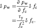
where μ = f c /α is the stress factor that represents the ratio of dry (p w = 0) basal shear traction to gravitational driving stress. Over the timescales of interest, it is reasonable to think of μ as the static stress component and (1 − p′w) as the dynamic component. That basal slip arises from unbalanced basal shear traction and driving stress requires the basal slip parameter, Θ, to be positive for basal slip to occur. Because basal shear traction can be less than the bed yield stress, we apply H(Θ), the Heavyside step function (H(Θ) = 1 for Θ >0 and H(Θ) = 0 otherwise), in Eqn (4) to ensure u′b is everywhere non-negative and real for any n. This condition provides some insight as to when certain glaciers accelerate in response to variations in basal water pressure. Setting Θ = 0 (i.e. τ d = τ y) yields the critical water pressure;
 $$p_{\rm w}^{\ast} = \rho gh\,(1 - {\mu ^{ - 1}}),$$
above which basal slip is non-zero. Only basal water pressure variations above the critical water pressure will lead to glacier flow variability.

Basal water pressure is equal to critical water pressure whenever gravitational driving stress is equal to the yield stress of the bed. During winter on Hofsjökull, inferred basal shear traction and driving stress are roughly balanced in areas with high basal slip rates (Fig. 7g). Consequently, inferred wintertime basal water pressure (Fig. 6i) and critical water pressure (Eqn (5)) should be approximately equal as well. Indeed we find good agreement between $p_{\rm w}^* $
and wintertime p
w in areas with basal slip rates above 4 cm d−1 (Fig. 8b). This agreement suggests that estimates of annually averaged, effective water pressures for broad spatial areas (several ice thicknesses) can be gleaned from surface slope and thickness measurements on glaciers that are at or near steady state.
$p_{\rm w}^* $
and wintertime p
w in areas with basal slip rates above 4 cm d−1 (Fig. 8b). This agreement suggests that estimates of annually averaged, effective water pressures for broad spatial areas (several ice thicknesses) can be gleaned from surface slope and thickness measurements on glaciers that are at or near steady state.
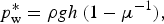
For sub-annual water pressure variations, our basal slip model (Eqn (4)) shows that the sensitivity of basal slip rate to changes in mean basal water pressure is given as:
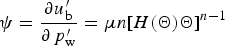 $$\psi = \displaystyle{{\partial {u^{\prime}_{{{\rm b}}}}} \over {\partial {\,p^{\prime}_{{\rm w}}}}} = \mu n{\left[ {H(\Theta )\Theta} \right]^{n - 1}}$$
and scales as the inverse of the ice surface slope. Published values give 0.3 ≤ f c ≤ 0.5, with f c being approximately constant in time (Iverson, Reference Iverson2010), while observed surface slopes vary by up to two orders of magnitude, with minimum values ~ 10−3, and may change on multi-annual timescales. Therefore, ice surface slope is the dominant factor in μ at seasonal and shorter timescales. Consequently, for a given f c, glaciers with gentler surface slopes require higher mean basal water pressures to initiate slip but, once slip has commenced, these glaciers are highly sensitive to subsequent changes in water pressure. This behavior is due to the dependence of basal slip rate on the ratio τ b/τ d: for a given ice thickness, glaciers with gentle surface slopes have relatively low gravitational driving stress, τ d, requiring basal water pressure to approach ice overburden pressure (i.e. for the glacier to approach floatation) for basal slip to commence. Once basal slip is underway, basal slip rates become increasingly sensitive to changes in water pressure as basal slip rates increase (Fig. 8a) because shearing in the glacier sidewalls is a fundamental control on ice flow in our model. A consequence of nonlinearity in ψ is that for a given change in the absolute value of mean basal water pressure (|δp w|) the amplitude of increases in basal slip rate (|δu b(δpw >0)|) will exceed the amplitude of decreases in basal slip rate (i.e. |δu b(δpw <0)| <|δu b(δpw >0)|). Furthermore, that ψ scales as the inverse of ice surface slope helps explain some of the variable response to meltwater flux on Hofsjökull, where typical surface slopes are <0.2, with a median of 0.06, making 2 ≤ μ ≤ 12 for f c = 0.4 (Fig. 9).
Stress factor μ for Hofsjökull calculated assuming f c = 0.4 and with surface slopes averaged over ~10 ice thicknesses. Blue contours delineate the bright regions in Figures 6i–p, indicating that basal slip occurs in these areas.

The sensitivity of basal slip rate to changes in basal water pressure can be understood in a Mohr's circle framework (Fig. 10), which considers the relationship between shear stress and effective normal stress (Malvern, Reference Malvern1969). In the idealized model, effective normal stress is equal to effective pressure N, where N = p
i − p
w and p
i = ρgh. For basal slip, we consider the gravitational driving stress and the basal shear tractions, which form the radii of the concentric half-circles labeled D, for driving stress (green), and B, for basal shear traction (red). We delineate the Mohr-Coulomb criteria (Eqn (2)) using the line labeled ‘yield criteria’, which slopes at an angle $\phi = \mathop {\tan} \nolimits^{ - 1} ({f_{\rm c}})$
. The value of τ
d dictates the maximum size of the half-circles because the Mohr-Coulomb criteria, along with the existence of non-zero stresses within the ice, requires B to be smaller than D at all times. Over the timescales of interest, τ
d is constant and τ
b is bounded by the bed yield stress. Thus half-circle D can enter the gray-shaded region but half-circle B cannot and B intersects the yield line at
$\phi = \mathop {\tan} \nolimits^{ - 1} ({f_{\rm c}})$
. The value of τ
d dictates the maximum size of the half-circles because the Mohr-Coulomb criteria, along with the existence of non-zero stresses within the ice, requires B to be smaller than D at all times. Over the timescales of interest, τ
d is constant and τ
b is bounded by the bed yield stress. Thus half-circle D can enter the gray-shaded region but half-circle B cannot and B intersects the yield line at ${p_{\rm w}}\, = \,p_{\rm w}^{\ast} $
.
${p_{\rm w}}\, = \,p_{\rm w}^{\ast} $
.
Mohr's circle representation of basal shear traction and driving stress, where $\phi = \mathop {\tan} \nolimits^{ - 1} ({f_{\rm c}})$
is the internal friction angle, N = p
i
− p
w is the effective pressure at the bed, assumed equal to the effective normal stress; p
i
= ρgh, the ice overburden pressure; and c
0 is the till cohesion, assumed negligible in Eqn (2).
$\phi = \mathop {\tan} \nolimits^{ - 1} ({f_{\rm c}})$
is the internal friction angle, N = p
i
− p
w is the effective pressure at the bed, assumed equal to the effective normal stress; p
i
= ρgh, the ice overburden pressure; and c
0 is the till cohesion, assumed negligible in Eqn (2).

The disparity between driving stress and basal shear traction in their response to yielding informs the sensitivity of basal slip rate to changes in basal water pressure. When τ
b < τ
y, both circles have approximately the same radius. Decreasing α reduces τ
d, shrinking half-circle D. If we hold f
c constant, then glaciers with smaller α will have greater freedom to traverse along the x-axis (effective normal stress) without their stress circles intersecting the yield line, meaning that $p_{\rm w}^* $
is large, as expected from Eqn (5). Once the bed beneath a shallow-sloping glacier begins to yield, there is less space between N at yielding and the origin where
$p_{\rm w}^* $
is large, as expected from Eqn (5). Once the bed beneath a shallow-sloping glacier begins to yield, there is less space between N at yielding and the origin where ${u_{\rm b}}\, = \,{u_{{{\rm b}_{{\rm max}}}}}$
, meaning that ψ must be large. Conversely, increasing α enlarges half-circle D causing the Mohr circles to intersect the yielding criteria at higher values of N (lower
${u_{\rm b}}\, = \,{u_{{{\rm b}_{{\rm max}}}}}$
, meaning that ψ must be large. Conversely, increasing α enlarges half-circle D causing the Mohr circles to intersect the yielding criteria at higher values of N (lower $p_{\rm w}^* $
) than for shallower-sloping glaciers, requiring relatively large subsequent increases in p
w to achieve
$p_{\rm w}^* $
) than for shallower-sloping glaciers, requiring relatively large subsequent increases in p
w to achieve ${u_{\rm b}}\, = \,{u_{{{\rm b}_{{\rm max}}}}}$
(i.e. ψ is small). We can achieve the same effect by increasing (decreasing) f
c instead of decreasing (increasing) α. Hence the sensitivity of basal slip rate to changes in basal water pressure scales as μ.
${u_{\rm b}}\, = \,{u_{{{\rm b}_{{\rm max}}}}}$
(i.e. ψ is small). We can achieve the same effect by increasing (decreasing) f
c instead of decreasing (increasing) α. Hence the sensitivity of basal slip rate to changes in basal water pressure scales as μ.
Together, spatial variability in μ (Fig. 9) and inferred basal water pressure (Figs 6i–p) more closely represent patterns in seasonal velocity (Figs 2a–c) than either individually. Outlet glaciers on Hofsjökull that show the greatest decrease in speed during the early melt season have the lowest μ values due to steep ice surface slopes. Outlet glaciers that experience nearly complete cessation of the observed acceleration within 10 d have μ<5 (Fig. 9) and show sharp reductions in basal water pressure (Figs 6j–k and n–o). Conversely, outlet glaciers that maintained elevated ice flow between early and mid-June 2012 have relatively high μ values due to gradual surface slopes, except for Illviðrajökull, whose basal hydrological system likely did not become channelized. Glaciers in the southeast quadrant, which have relatively high μ values, sustain increased speeds during the period of observation despite modestly elevated basal water pressures.
These observations indicate that the stress factor, μ, is a useful parameter in establishing a glacier's dynamic response to basal water flux. Glaciers accelerate in response to rapid changes in melting or precipitation so long as basal water pressure exceeds the critical water pressure (Eqn (5)), a function of ice overburden pressure and μ. Initial melt-season accelerations may be ephemeral owing to evolving hydrological systems but diurnal melt cycles and periodic rain events can continue to episodically overwhelm and pressurize the system throughout the melt season. Ice flow responds readily to these continual, short-term water pressure fluctuations (Shepherd and others, Reference Shepherd2009; Schoof, Reference Schoof2010) and this response will be amplified on glaciers with gentle surface slopes. Longer melt seasons, increasing diurnal temperature variations and more frequent rain events (e.g. Schuenemann and Cassano, Reference Schuenemann and Cassano2010) brought on by a warming climate will potentially bolster total melt-season mass flux in gently sloping glaciers, while glaciers with steep surface slopes will be less susceptible to these prolonged cyclical basal water pressure variations. Given the prevalence of till-covered glacier beds, these findings should help reconcile observations of the influence of basal hydrology and surface meltwater flux on glacier flow (Zwally and others, Reference Zwally2002; Joughin and others, Reference Joughin2008; Shepherd and others, Reference Shepherd2009; Bartholomew and others, Reference Bartholomew2010; Moon and others, Reference Moon2014; Tedstone and others, Reference Tedstone2013, Reference Tedstone2015). In particular, it may be useful to classify glaciers by μ to facilitate mechanistically consistent comparisons of the response of different glaciers with surface meltwater flux and enhance our understanding of basal processes.
Our model has some limitations in its immediate applicability to understanding the response of soft-bedded glaciers to surface meltwater flux. The primary limitation is that not all glaciers closely adhere to the idealized assumptions employed in the model derivation. More robust testing with numerical models and further observations on other glacier systems are needed to support the model and lend credence to μ as a viable mechanistic parameter. Another limitation is the need to decouple the dependence of ψ and the evolution of the basal hydrological system on the ice surface slope in observations (e.g. Schoof, Reference Schoof2010). These mechanical and hydrological dependencies work together, with gentler surface slopes potentially resisting channelization of the hydrological system by increasing the critical meltwater flux needed to facilitate the switch from an inefficient distributed system to an efficient channelized system. This resistance to channelization increases the likelihood that an inefficient distributed hydrological system will persist later in the melt season on shallower-sloping glaciers, resulting in higher basal water pressure variability (Schoof, Reference Schoof2010) in a system with higher dynamical sensitivity to such variability (Eqn (6)). Because it may not be possible to know the state of the basal hydrological system during the early melt season, collecting observations aimed at understanding ψ is challenging. In this work, we avoid the complexities of evolving basal hydrological systems by estimating the effective basal water pressure directly from observations of surface velocity and the inferred basal shear traction fields. Our approach isolates the mechanical basal properties from the hydrological properties, providing insight into the mechanics of deformable glacier beds.
Improved understanding of basal mechanics is a key component of the physical foundation on which we can build predictive models to explore a range of plausible future glacier states in a warming climate. One outstanding problem currently prohibiting reliable predictive models is an incomplete understanding of how changes in water flux at the bed of glaciers, arising from surface meltwater flux, transmission of tidal loads (e.g. Thompson and others, Reference Thompson, Simons and Tsai2014) or subglacial lake drainage (e.g. Magnússon and others, Reference Magnússon, Rott, Björnsson and Pálsson2007, Reference Magnússon, Björnsson, Rott and Pálsson2010; Fricker and Scambos, Reference Fricker and Scambos2009), influences multi-annual-timescale ice flow. Solving this problem requires defining the sensitivity of basal slip rate to changes in q w, the water flux through the basal hydrological system, given as:
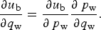 $$\displaystyle{{\partial {u_{\rm b}}} \over {\partial {q_{\rm w}}}} = \displaystyle{{\partial {u_{\rm b}}} \over {\partial {\,p_{\rm w}}}}\displaystyle{{\partial {\,p_{\rm w}}} \over {\partial {q_{\rm w}}}}.$$
The second term on the right hand side of Eqn (7) (∂p
w/∂q
w) is a function of the time-varying state of the basal hydrological system and is the subject of numerous studies (e.g. Lliboutry, Reference Lliboutry1968; Röthlisberger, Reference Röthlisberger1972; Nye, Reference Nye1976; Kamb, Reference Kamb1987; Schoof, Reference Schoof2010). With this study, we define the first term on the right hand side of Eqn (7), simply the dimensional form of Eqn (6) in which both sides are multiplied by ${u_{{{\rm b}_{{\rm max}}}}}/(\rho gh)$
, in an idealized framework for glaciers with deformable beds.
${u_{{{\rm b}_{{\rm max}}}}}/(\rho gh)$
, in an idealized framework for glaciers with deformable beds.
5 CONCLUSION
We use InSAR-derived measurements of ice surface velocity combined with a numerical ice-flow model to study the response of several outlet glaciers on Hofsjökull ice cap to surface melt during the early melt season. Observations indicate that the outlet glaciers respond differently to similar environmental forcing with some glaciers maintaining fast ice flow relative to winter while other glaciers appear to accelerate then slow to wintertime speeds over the same time period. This spatial heterogeneity in the response of ice flow to surface melt is at least partially explained by differential evolution of the basal hydrological systems of the outlet glaciers, which influences how surface meltwater flux can alter basal shear traction and consequently ice flow. We infer basal shear tractions using the observed velocities and note that the bed beneath Hofsjökull deforms plastically, allowing for a straightforward means of estimating absolute and seasonally variable basal water pressures. The resulting water pressure estimates indicate that changes in basal water pressure and surface velocity are non-local and nonlinearly related. These findings motivate an idealized model of basal slip rate wherein the response of glaciers with plastically deforming beds is largely determined by the relationship between the intrinsic mechanical properties of the deforming bed and glacier geometry. This relationship is quantified by the stress factor, μ, defined as the ratio of the internal friction parameter for the bed to the ice surface slope.
In plastic-bedded glaciers, μ helps determine the critical basal water pressure, $p_{\rm w}^* $
, at which basal slip commences and the sensitivity of basal slip rate to changes in basal water pressure. Given the ranges of plausible values for internal friction in till and ice surface slopes, both the critical water pressure and sensitivity of basal slip rate to changes in basal water pressure are driven primarily by the ice surface slope. Glaciers with shallower ice surface slopes require higher basal water pressure (relative to overburden pressure) for incipient basal slip, but basal slip rate is then more sensitive to basal water pressure variations than in steeper sloping glaciers. Our observations support this conclusion by showing that outlet glaciers that maintained elevated ice flow between early and mid-June, despite evidence that the respective hydrological systems evolved toward being channelized, have relatively high μ values, arising from gentle surface slopes. Conversely, outlet glaciers that experienced the greatest slowdowns over the same time period have relatively low μ values, or steep surface slopes.
$p_{\rm w}^* $
, at which basal slip commences and the sensitivity of basal slip rate to changes in basal water pressure. Given the ranges of plausible values for internal friction in till and ice surface slopes, both the critical water pressure and sensitivity of basal slip rate to changes in basal water pressure are driven primarily by the ice surface slope. Glaciers with shallower ice surface slopes require higher basal water pressure (relative to overburden pressure) for incipient basal slip, but basal slip rate is then more sensitive to basal water pressure variations than in steeper sloping glaciers. Our observations support this conclusion by showing that outlet glaciers that maintained elevated ice flow between early and mid-June, despite evidence that the respective hydrological systems evolved toward being channelized, have relatively high μ values, arising from gentle surface slopes. Conversely, outlet glaciers that experienced the greatest slowdowns over the same time period have relatively low μ values, or steep surface slopes.
ACKNOWLEDGEMENTS
The authors benefited from discussions with R. Arthern, H. Gudmundsson, I. Hewitt, J.-P. Ampuero, T. Johannesson, and T. van Boeckel. We thank Y. Lou, B. Hawkins, Y. Zheng, and the UAVSAR crew for assistance with InSAR data collection and processing, T. Johannesson, on behalf of the Icelandic Meteorological Office, provided the Hofsjökull DEM. This research was conducted at the California Institute of Technology and the University of Iceland with funding provided by the NASA Crysopherice Sciences Program (Award NNX14AH80G). B. M. was partially funded by a NASA Earth and Space Sciences Fellowship and an Achievement Rewards for College Students (ARCS) fellowship. InSAR data are freely available from the Alaska Satellite Facility via the UAVSAR website (http://uavsar.jpl.nasa.gov).


 Open access