


Nomenclature
- ${T_{{\theta _2}}}$
-
short period time constant
-
${x_{cg}}$
-
centre of gravity
- CAP
-
control anticipation parameter
- CAS
-
calibrated airspeed
- CoG
-
centre of gravity
- DI
-
dynamic inversion
- f, g
-
unknown nonlinear functions
- FQ
-
flight quality
- ICAO
-
International Civil Aviation Organization
- LOC-II
-
loss-of-control in flight
- LOE
-
loss-of-effectiveness
- NDI
-
nonlinear dynamic inversion
- NN
-
neural network
- PID
-
proportional integral derivative
- RAFS
-
research aircraft flight simulator
- RLS
-
recursive least square
-
${\mathbf{F}},\,{{\hat {\mathbf{F}}}}$
-
local state matrix and its estimate, respectively
-
${\mathbf{G}},\,{{\hat {\mathbf{G}}}}$
-
local control matrix and its estimates, respectively
-
${\mathbf{I}}$
-
unit matrix
-
${\mathbf{L}}$
-
covariance matrix
-
${\mathbf{V}},{\rm{\;}}\mathbf{W}$
-
neural network weight matrices
-
$m{\rm{\;}}$
-
mass
-
$q$
-
pitch rate
-
$u,{\rm{\;}}v,{\rm{\;}}w$
-
velocity components


Greek symbol
-
${\delta _e}$
-
elevator deflection
-
${\xi _{sp}}$
-
short period damping
-
${\omega _{sp}}$
-
short period natural frequency
-
${\boldsymbol{\Delta }}t$
-
time step
-
${\boldsymbol{\Gamma }}$
-
learning rate matrix
-
${\boldsymbol{\Theta }},\,{{\hat {\boldsymbol{\Theta}} }}$
-
matrix of unknown parameters and its estimate
-
$\theta $
-
pitch angle
-
$\kappa $
-
forgetting factor
-
$\lambda $
-
scalar
-
$\sigma ,{\rm{\;}}\sigma^\prime $
-
sigmoid transfer function and its gradient
-
$\unicode{x1D6D7}$
-
unknown nonlinear function
-
$\epsilon $
-
RLS estimation error


1.0 Introduction
Flight control systems are critical for maintaining stability and safety in aircraft operations. According to the Federal Administration Aviation (FAA), human errors contribute to nearly 60% to 80% of aircraft accidents [1], which are often due to unmitigated environmental hazards or system failures. Advanced flight control laws therefore play a central role in reducing pilot workload, enhancing autonomy and improving operational safety. Compared to costly structural modifications, software-based enhancements at the control level, such as flutter suppression or manoeuvre load alleviation, provide more flexible and efficient solutions [Reference Wunderlich, Dähne, Reimer and Schuster2]. This motivates the development of adaptive and intelligent controllers that can reliably handle uncertainties in real time.
Traditional flight control architectures still primarily rely on linear controllers such as proportional integral derivative (PID) and linear quadratic regulator (LQR) designs [Reference Stevens, Lewis and Johnson3]. These methods are straightforward and well-established offering proven stability with guaranteed gain and phase margins. However, they require precise gain scheduling [Reference Reynolds, Pachter and Houpis4] to ensure adequate performance across the aircraft’s full envelope and under varying operating conditions. The tuning of these controllers is based on linearised models, which often neglect higher-order nonlinearities [Reference Stevens, Lewis and Johnson3]. Consequently, performance degrades and stability margins may deteriorate when the aircraft operates outside the scheduled regime. Robust control techniques such as ${H_\infty }$
[Reference Khalil and Fezans5, Reference Efremov, Mbikayi and Efremov6] and linear quadratic Gaussian (LQG) controllers [Reference Ferrier, Nguyen, Ting, Chaparro, Wang, de Visser and Chu7] mitigate certain uncertainties, but they are still strongly dependent on accurate mathematical models.
${H_\infty }$
[Reference Khalil and Fezans5, Reference Efremov, Mbikayi and Efremov6] and linear quadratic Gaussian (LQG) controllers [Reference Ferrier, Nguyen, Ting, Chaparro, Wang, de Visser and Chu7] mitigate certain uncertainties, but they are still strongly dependent on accurate mathematical models.
Advanced nonlinear control methods, such as nonlinear dynamic inversion (NDI) [Reference Horn8–Reference Steffensen, Steinert and Smeur10] and model predictive control (MPC) [Reference Doff-Sotta, Cannon and Bacic11], address several of the limitations of traditional linear techniques. However, both approaches depend heavily on precise state-space models [Reference Harris, Elliott and Tallant12–Reference Eren, Prach, Koçer, Raković, Kayacan and Açıkmeşe14], making them sensitive to parameter variations, unmodeled dynamics or environmental disturbances. This reliance on precise linearisation remains one of the main obstacles to their widespread application in commercial aircraft.
To mitigate this dependence, online estimation techniques such as recursive least squares (RLS) [Reference Haykin15–Reference Mohseni and Bernstein17] and extended Kalman filtering (EKF) [Reference Xiaoqian, Feicheng, Zhengbing and Hongying18] have been developed, enabling incremental model updates [Reference Konatala, Milz, Weiser, Looye and van Kampen19] and adaptive compensation of the dynamic inversion [Reference Andrianantara, Ghazi and Botez20–Reference Nguyen22] or MPC controllers [Reference Andrianantara, Ghazi and Botez23]. Although effective in principle, their performance is often sensitive to initialisation conditions, forgetting factor selection, and numerical instabilities, which can compromise real-time implementation.
In parallel, intelligent control approaches have demonstrated the ability of neural networks [Reference Ge, Hang, Lee and Zhang24–Reference Emami, Castaldi and Banazadeh26], fuzzy logic [Reference Grigorie, Botez, Popov, Mamou and Mébarki27–Reference Hosseini, Ghazi and Botez29] and hybrid adaptive controllers [Reference Pedro and Meyer30–Reference Lungu, Lungu and Efrim32] to capture nonlinearity and compensate for unmodeled dynamics. Robust adaptive control, in particular, has raised interests due to its effectiveness in compensating for time-varying dynamics and in controlling highly nonlinear systems, including actuator dynamics [Reference Steffensen, Steinert and Smeur10].
Foundational works by Ref. [Reference Nguyen22] introduced hybrid adaptive control architectures that combines baseline inversion controllers, indirect parameter estimation using RLS and adaptive neural networks adaptive controllers for compensation [Reference Nguyen22–Reference Park, Shin, Lee and Antonios33]. These studies validated the hybrid concept for damaged aircraft and launch vehicles [Reference Nguyen and Krishnakumar34]. More recent applications on the Cessna Citation X [Reference Andrianantara, Ghazi and Botez20–Reference Andrianantara, Ghazi and Botez23] have demonstrated the potential of dynamic inversion combined with neural network controllers. However, while these studies established the foundation for hybrid adaptive dynamic inversion, their scope was limited in terms of flight conditions and did not address certification-level validation. This study extends their findings by systematically analysing RLS estimation sensitivity, integrating neural networks adaptive learning and demonstrating Level 1 flight qualities under FAA standards.
This paper advances the state of the art by implementing a hybrid RLS – NN adaptive controller for the longitudinal pitch-rate control of the Cessna Citation X. Unlike prior studies, the controller is designed and validated across 64 flight conditions covering the aircraft cruise envelope, thereby removing the need to gain scheduling. In this architecture, the baseline PID controller operates with fixed gains to provide stability, while only the RLS estimator and NN residual compensator adapt online. This design eliminates the need for repeated across conditions, as adaptation is handled automatically by the adaptive controllers. Furthermore, this study provides a systematic analysis of RLS adaptation mechanisms, including initialisation, forgetting factors and covariance resets, and evaluates their impact on both stability and accuracy. Neural networks are then integrated for direct control, providing robust adaptation even in case of degraded RLS estimates. Importantly, flight qualities are explicitly validated, showing Level 1 compliance [Reference Hakim and Choukri35–Reference Hodgkinson37], while nonlinear stability is formally guaranteed through Lyapunov-based analysis [Reference Narendra and Annaswamy38, Reference Lewis, Yeşildirek and Liu39].
Related controller structures with different compensation strategies have been assessed by other researchers. Steffensen et al. [Reference Steffensen, Steinert and Smeur10] examined nonlinear dynamic inversion (DI) with incremental control perspectives, including first-order actuator dynamics, showing improved robustness but without NN augmentation nor analysis of wide-range uncertainties. Harris et al. [Reference Harris, Elliott and Tallant12] applied L1 adaptive DI ensuring fast adaptation but with a strong dependence on accurate modelling and without formal flight quality assessment. More recently, Andrianantara et al. [Reference Andrianantara, Ghazi and Botez23] extended their earlier study by combining MPC with RLS and NN augmentation for the Cessna Citation X, demonstrating performance gains but without systematic RLS estimator tuning or robustness validation. In contrast, the present study incorporates higher-order actuator dynamics, introduces a formal tuning methodology and conducts comprehensive robustness testing. Taken together, these contributions help bridge the gap between theoretical adaptive controller designs and certifiable implementations suitable for commercial aircraft.
Several researchers have focused their efforts on unmanned aerial vehicle (UAV) applications, where agility and adaptability are prioritised over certifiability. This is made possible due to the fact that UAVs present less risk to human life, as being remotely controlled. O’Connell et al. [Reference O’Connell, Shi, Shi, Azizzadenesheli, Anandkumar, Yue and Chung40] demonstrated rapid NN-based adaptation for UAV flight in strong winds, but relied primarily on reinforcement learning without model-based stability guarantees. Zhou et al. [Reference Zhou, Ho and Chu41] proposed extended incremental DI with optical-flow feedback for micro air vehicles, confirming feasibility but only in small-scale systems. Earlier, Pedro and Meyer [Reference Pedro and Meyer30] applied NN-based DI to fighter aircraft, showing improved nonlinear tracking in simulations but without robustness validation. Similarly, Lungu and Lungu [Reference Lungu and Lungu31] applied NN – DI to landing autopilots, enhancing robustness during approach and flare, while Lungu et al. [Reference Lungu, Lungu and Efrim32] later extended NN – DI concepts to spacecraft control. These studies confirm the adaptability of NN-augmented DI across various domains; however, they are limited to UAV-scale or highly specific applications. This study, instead, focuses on manned commercial aircraft, for which a high-fidelity research aircraft flight simulator is available, thereby extending NN – DI hybrid approaches into a certifiable, envelope-wide framework.
In summary, the benefits of the proposed controller are twofold. First, the architecture is simplified, since gain-scheduled controllers are replaced by a single adaptive configuration capable of covering the entire cruise envelope. Second, the controller demonstrates robustness against a wide range of uncertainties, including turbulence, actuator loss-of-effectiveness and actuator noise, while maintaining compliance with flight quality requirements.
By addressing long-standing limitations related to gain scheduling, model dependence and estimator sensitivity, this work provides a practical and certifiable method for integrating intelligent adaptive controllers into commercial aircraft. While previous studies [Reference Steffensen, Steinert and Smeur10–Reference Harris, Elliott and Tallant12] have validated adaptive NN – DI concepts in specific operating conditions, UAVs, or specialised mission phases, this study systematically assesses 64 cruise conditions of the Cessna Citation X, integrates NN residual learning with RLS sensitivity analysis, incorporates higher-order actuator dynamics and validates flight qualities against FAA Level 1 standards. This represents a significant step beyond feasibility demonstrations and aligns with ongoing certification initiatives from the FAA, EASA and NASA [42–Reference Agogino, Brat, He, Hulse, Lipkis, Pressburger, Gopinath, Irshad, Katis and Mavridou44], thereby reinforcing both the relevance and applicability of the proposed approach.
The remainder of this paper is organised as follows: Section 2 presents the methodology and controller design; Section 3 details the tuning strategy and results for ideal conditions; Section 4 provides robustness evaluation; Section 5 discusses findings; and Section 6 concludes with final remarks. The Lyapunov stability assessment is provided in the appendix.
1.1 Aircraft model and simulation platform
1.1.1 Cessna Citation X aircraft specifications
The Cessna Citation X is a long-range business jet that has been widely used as a platform for advanced control design [Reference Andrianantara, Ghazi and Botez23–Reference Hosseini, Ghazi and Botez29]. Since its introduction in 1996, the business jet aircraft has been recognised as one of the fastest business jets ever produced, with a maximum cruise speed of 350 kn and a maximum Mach number of 0.92. The aircraft is powered by two Rolls-Royce AE3007C-1 turbofan engines, each providing a maximum thrust of 28,655 N. Its cabin accommodates up to 12 passengers and three crew members.
The Cessna Citation X has a maximum range of 5,724 km and a service ceiling of 15,544 m. Its main performance characteristics, summarised in Table 1, make the Cessna Citation X an excellent candidate for adaptive control studies. In fact, its wide and available operational envelope, high performance and high-fidelity simulation models [Reference Ghazi and Botez45] provide a realistic platform for evaluating adaptive flight control architectures.
Cessna Citation X flight specifications

1.1.2 Nonlinear Simulink platform
A high-fidelity nonlinear model of the Cessna Citation X was developed in MATLAB/Simulink [Reference Ghazi and Botez45] and serves as a research platform for the controller design. This Simulink model integrates several modules such as aerodynamics, engine dynamics, actuator and sensor dynamics, atmospheric disturbance effects and other relevant aircraft systems.
The Simulink model was cross-validated using simulated flight data from a Research Aircraft Flight Simulator (RAFS) of the Cessna Citation X, designed and manufactured by CAE Inc. [Reference Ghazi and Botez45] and shown in Fig. 1. The RAFS has been validated by CAE engineers, based on qualification test guide (QTG) procedures and real flight-test data from the Cessna Citation X. In addition, the RAFS satisfies the flight simulator validation criteria imposed by the Federal Aviation Administration (FAA) and can be considered comparable to Level D fidelity with respect to flight dynamics. The flight dynamics implemented within the RAFS are based on CAE Inc. and Cessna Aircraft (Textron) proprietary data and are therefore not publicly accessible. However, the RAFS provides access to high-fidelity simulated flight data and supports the execution of a wide range of flight scenarios, manoeuvres and full-mission simulations. The MATLAB/Simulink environment was developed to reproduce the RAFS flight dynamics with sufficient accuracy to support advanced control design, thereby ensuring that controller development and evaluation are conducted on high-fidelity flight dynamics.
Cessna Citation X research aircraft flight simulator (RAFS) manufactured by CAE Inc.

In addition, the Cessna Citation X simulation platforms, both the RAFS and the derived Simulink models, have been widely used in advanced control research and peer-reviewed research literature. Examples of application include NN-based adaptive controllers with approximate dynamic inversion [Reference Andrianantara, Ghazi and Botez20, Reference Quintin, Andrianantara, Ghazi and Botez21] and model predictive controllers [Reference Eren, Prach, Koçer, Raković, Kayacan and Açıkmeşe14]. Similarly, fuzzy logic and recurrent neural network controllers have been demonstrated for longitudinal and lateral control [Reference Hosseini, Ghazi and Botez29–Reference Hosseini, Bematol, Ghazi and Botez51], while control clearance and lateral flight qualities were investigated in [Reference Boughari, Botez, Ghazi and Theel49, Reference Boughari, Ghazi, Botez and Theel50].
1.2 Nonlinear dynamic model
1.2.1 Cessna Citation X nonlinear dynamic model
The aircraft’s longitudinal dynamics were considered in this study. This assumption allows us to write the following nonlinear representation of the aircraft’s longitudinal dynamics:
 \begin{align}\begin{array}{l}{\dot {\mathbf{x}}} = {\unicode{x1D6D7}}( {{\mathbf{x}},\eta } )\\y = h( {\mathbf{x}} )\end{array} \end{align}
where ${\mathbf{x}} = {[ u \quad w \quad q \quad \theta ]^T}$
is the state vector,
${\mathbf{x}} = {[ u \quad w \quad q \quad \theta ]^T}$
is the state vector, $u$
and
$u$
and $w{\rm{\;}}$
are the longitudinal and lateral velocity components, respectively,
$w{\rm{\;}}$
are the longitudinal and lateral velocity components, respectively, $q$
is the pitch rate
$q$
is the pitch rate $\theta $
is the pitch angle,
$\theta $
is the pitch angle, $h$
is a nonlinear function,
$h$
is a nonlinear function, ${\rm{\;}}\eta = {\delta _e}$
is the elevator input and
${\rm{\;}}\eta = {\delta _e}$
is the elevator input and $\unicode{x1D6D7}$
is an unknown nonlinear function.
$\unicode{x1D6D7}$
is an unknown nonlinear function.
1.2.2 Nonlinear actuator dynamics
The actuators are modelled in Simulink using a second-order nonlinear transfer function. This allows us to realistically reproduce the higher-order nonlinearity that strongly affect aircraft stability and control performance, particularly in adaptive flight control studies [Reference Steffensen, Steinert and Smeur10]. The actuator parameters are summarised in Table 2.
Actuator dynamics parameter

2.0 Pitch rate controller design
2.1 Controller architecture
Figure 2 presents the controller architecture for the pitch rate control. The control elements include a baseline PID controller, an RLS-based DI controller and a NN adaptive controller. The stability analysis is detailed in the appendix.
Pitch rate model reference adaptive controller using PID, RLS dynamic inversion and adaptive NN.

Controlling the pitch rate $q$
for longitudinal control aims to track the desired short period performances [Reference Stevens, Lewis and Johnson3]. Therefore, the proposed control algorithm is designed to track a reference signal
$q$
for longitudinal control aims to track the desired short period performances [Reference Stevens, Lewis and Johnson3]. Therefore, the proposed control algorithm is designed to track a reference signal ${q_{ref}}$
.
${q_{ref}}$
.
2.2 Controller elements
Nonlinear Dynamic Inversion Controller
For linear systems, DI is straightforward to execute [Reference Stevens, Lewis and Johnson3]. For nonlinear systems, the inversion is more difficult, as nonlinear systems may include unmodeled dynamics. According to Ref. [Reference Stevens, Lewis and Johnson3], most aircraft dynamics can be represented in affine form, with respect to the control input. Therefore, Equation (1) can be rewritten as:
 \begin{align}\begin{array}{l}{\dot {\mathbf{x}}} = {\mathbf{f}}( {\mathbf{x}} ) + {\mathbf{g}}( {\mathbf{x}} )\eta \\y = q = {\mathbf{Cx}}\end{array} \end{align}
where ${\rm{f}}$
and
${\rm{f}}$
and ${\mathbf{g}}$
are nonlinear functions, and
${\mathbf{g}}$
are nonlinear functions, and ${\rm{y}}$
is the output. Hence,
${\rm{y}}$
is the output. Hence, $\rm{C} = [ 0\quad {}0\quad {}1\quad {}0]$
for pitch rate output.
$\rm{C} = [ 0\quad {}0\quad {}1\quad {}0]$
for pitch rate output.
Inverting Equation (1), the control input may be written as:
 \begin{align}{\rm{\eta }} = \aleph ( {\dot {\mathbf{x}},\mathbf{x}} ) \end{align}
where $\aleph = {{\unicode{x1D6D7}}^{ - 1}}$
is the inverse function of
$\aleph = {{\unicode{x1D6D7}}^{ - 1}}$
is the inverse function of ${\unicode{x1D6D7}}$
. Next, let’s express
${\unicode{x1D6D7}}$
. Next, let’s express ${\rm{\eta }} = {{\rm{\delta }}_{\rm{e}}}$
according to the control algorithm in Fig. 2. Considering Equations (1) and (2):
${\rm{\eta }} = {{\rm{\delta }}_{\rm{e}}}$
according to the control algorithm in Fig. 2. Considering Equations (1) and (2):
 \begin{align}{\dot {\mathbf{x}}} = {\unicode{x1D6D7}}( {{\mathbf{x}},{\rm{\eta }}} ) = {\rm{f}}( {\mathbf{x}} ) + {\mathbf{g}}( {\mathbf{x}} ){\rm{\eta }} \end{align}
Developing Equation (4) using the first-order linear approximation around ( ${{\mathbf{x}}_0},{\eta _0})$
, we obtain:
${{\mathbf{x}}_0},{\eta _0})$
, we obtain:
 \begin{align}{\unicode{x1D6D7}}( {{\mathbf{x}},{\rm{\eta }}} ) = {\unicode{x1D6D7}}( {{{\mathbf{x}}_0},{{\rm{\eta }}_0}} ) + {{{\unicode{x1D6D7}'}}_{\rm{x }}}{( {{\mathbf{x}},{\rm{\eta }}} )_{{{\mathbf{x}}_0},{{\rm{\eta }}_0}}}( {{\mathbf{x}} - {{\mathbf{x}}_0}} ) + {{\unicode{x1D6D7}^\prime}_{\rm{\eta }}}{( {{\mathbf{x}},{\rm{\eta }}} )_{{{\mathbf{x}}_0},{{\rm{\eta }}_0}}}( {{\rm{\eta }} - {{\rm{\eta }}_0}} ) \end{align}
where ${{\unicode{x1D6D7}}}( {{{\mathbf{x}}_0},{\eta _0}} )$
is the value at (
${{\unicode{x1D6D7}}}( {{{\mathbf{x}}_0},{\eta _0}} )$
is the value at ( ${{\mathbf{x}}_{\mathbf{0}}},{\eta _0})$
,
${{\mathbf{x}}_{\mathbf{0}}},{\eta _0})$
, ${{{\unicode{x1D6D7}'}}_x}{( {{\mathbf{x}},\eta } )_{{{\mathbf{x}}_0},{\eta _0}}}$
and
${{{\unicode{x1D6D7}'}}_x}{( {{\mathbf{x}},\eta } )_{{{\mathbf{x}}_0},{\eta _0}}}$
and ${{{\unicode{x1D6D7}'}}_\eta }{( {{\mathbf{x}},\eta } )_{{{\mathbf{x}}_0},{\eta _0}}}$
are the partial derivatives of
${{{\unicode{x1D6D7}'}}_\eta }{( {{\mathbf{x}},\eta } )_{{{\mathbf{x}}_0},{\eta _0}}}$
are the partial derivatives of ${{\unicode{x1D6D7}}}$
with respect to
${{\unicode{x1D6D7}}}$
with respect to ${\mathbf{x}}$
and
${\mathbf{x}}$
and $\eta $
, respectively. We may formulate the terms in Equation (5), such as:
$\eta $
, respectively. We may formulate the terms in Equation (5), such as:
 \begin{align}{{\unicode{x1D6D7}}}( {{{\mathbf{x}}_0},{\eta _0}} ) = {\mathbf{f}}( {{{\mathbf{x}}_0}} ) + {\mathbf{g}}( {{{\mathbf{x}}_0}} )\eta \end{align}
 \begin{align} {{{\unicode{x1D6D7}'}}_x}( {{\mathbf{x}},\eta } ) = \frac{{\partial {\mathbf{f}}( {\mathbf{x}} )}}{{\partial {\mathbf{x}}}} + \frac{{\partial {\mathbf{g}}( {\mathbf{x}} )}}{{\partial {\mathbf{x}}}}\eta \end{align}
 \begin{align}{{{\unicode{x1D6D7}'}}_\eta }( {{\mathbf{x}},\eta} ) = \frac{{\partial {\rm{f}}( {\mathbf{x}} )}}{{\partial {\rm{\eta }}}} + \frac{{\partial \left[ {{\mathbf{g}}( {\mathbf{x}} ){\rm{\eta }}} \right]}}{{\partial {\rm{\eta }}}} = {\mathbf{g}}( {\mathbf{x}} ) \end{align}
Considering the following changes, so that ${\boldsymbol{\Delta }}{\mathbf{x}} = \left( {{\mathbf{x}} - {{\mathbf{x}}_0}} \right){\rm{\;}}$
and
${\boldsymbol{\Delta }}{\mathbf{x}} = \left( {{\mathbf{x}} - {{\mathbf{x}}_0}} \right){\rm{\;}}$
and ${\boldsymbol{\Delta }}\eta = \left( {\eta - {\eta _0}} \right)$
, and substituting Equation (6) into Equation (5), the following expression is obtained:
${\boldsymbol{\Delta }}\eta = \left( {\eta - {\eta _0}} \right)$
, and substituting Equation (6) into Equation (5), the following expression is obtained:
 \begin{align}{{\unicode{x1D6D7}}}( {{\mathbf{x}},\eta } ) = {\mathbf{f}}( {{{\mathbf{x}}_0}} ) + {\mathbf{g}}( {{{\mathbf{x}}_0}} )\eta + {\left( {\frac{{\partial {\mathbf{f}}( {\mathbf{x}} )}}{{\partial {\mathbf{x}}}} + \frac{{\partial {\mathbf{g}}( {\mathbf{x}} )}}{{\partial {\mathbf{x}}}}\eta } \right)_{{{\mathbf{x}}_0},{\eta _0}}}{\mathbf{\Delta x}} + {\mathbf{g}}{( {\mathbf{x}} )_{{{\mathbf{x}}_0},{\eta _0}}}{\boldsymbol{\Delta }}\eta \end{align}
Let us express $\dot x$
in Equation (4) for small perturbations around
$\dot x$
in Equation (4) for small perturbations around $\left( {{{\mathbf{x}}_0},{\rm{\;}}{\eta _0}} \right)$
:
$\left( {{{\mathbf{x}}_0},{\rm{\;}}{\eta _0}} \right)$
:
 \begin{align}{\dot {\mathbf{x}}} = {{\dot {\mathbf{x}}}_0} + {{\Delta \dot {\mathbf{x}}}} = {{\unicode{x1D6D7}}}\left( {{\mathbf{x}},\eta } \right) \end{align}
From Equations (7) and (8), and considering ${{\dot {\mathbf{x}}}_0} = {\mathbf{f}}( {{{\mathbf{x}}_0}} ) + {\mathbf{g}}( {{{\mathbf{x}}_0}} )\eta $
,
${{\dot {\mathbf{x}}}_0} = {\mathbf{f}}( {{{\mathbf{x}}_0}} ) + {\mathbf{g}}( {{{\mathbf{x}}_0}} )\eta $
, ${\boldsymbol{\Delta }}{\dot {\mathbf{x}}}$
can be written such as:
${\boldsymbol{\Delta }}{\dot {\mathbf{x}}}$
can be written such as:
 \begin{align}{\boldsymbol{\Delta }}{\dot {\mathbf{x}}} = {\left( {\frac{{\partial {\mathbf{f}}( {\mathbf{x}} )}}{{\partial {\mathbf{x}}}} + \frac{{\partial {\mathbf{g}}( {\mathbf{x}} )}}{{\partial {\mathbf{x}}}}\eta } \right)_{{{\mathbf{x}}_0},{\eta _0}}}{\boldsymbol{\Delta }}{\mathbf{x}} + {\mathbf{g}}{( {\mathbf{x}} )_{{{\mathbf{x}}_0},{\eta _0}}}{\boldsymbol{\Delta }}\eta \end{align}
Making the following changes:
 \begin{align}{{\mathbf{F}}_{{{\mathbf{x}}_0},{\eta _0}}} = {\left( {\frac{{\partial {\mathbf{f}}\left( {\mathbf{x}} \right)}}{{\partial {\mathbf{x}}}} + \frac{{\partial {\mathbf{g}}\left( {\mathbf{x}} \right)}}{{\partial {\mathbf{x}}}}\eta } \right)_{{{\mathbf{x}}_0},{\eta _0}}};{\rm{\;}}{{\mathbf{G}}_{{{\mathbf{x}}_0},{\eta _0}}} = {\mathbf{g}}{\left( {\mathbf{x}} \right)_{{{\mathbf{x}}_0},{\eta _0}}} \end{align}
Equation (9) can be expressed in a simplified form:
 \begin{align}{\boldsymbol{\Delta }}{\dot {\mathbf{x}}} = {{\mathbf{F}}_{{{\mathbf{x}}_0},{\eta _0}}}{\mathbf{\Delta x}} + {{\mathbf{G}}_{{{\mathbf{x}}_0},{\eta _0}}}{\boldsymbol{\Delta }}\eta \end{align}
Recalling from Equation (2), ${\boldsymbol{\Delta }}\dot y$
may be computed as follows:
${\boldsymbol{\Delta }}\dot y$
may be computed as follows:
 \begin{align}{{\Delta \dot {\mathbf{y}}}} = {{C\Delta \dot {\mathbf{x}}}} \end{align}
Substituting ${{\Delta \dot {\mathbf{x}}}}$
from Equation (11) into Equation (12), we obtain:
${{\Delta \dot {\mathbf{x}}}}$
from Equation (11) into Equation (12), we obtain:
 \begin{align}{{\Delta \dot {\mathbf{y}}}} = {\mathbf{C}}{{\mathbf{F}}_{{{\mathbf{x}}_0},{{\rm{\eta }}_0}}}{{\boldsymbol{\Delta}} \mathbf{x}} + {\mathbf{C}}{{\mathbf{G}}_{{{\mathbf{x}}_0},{{\rm{\eta }}_0}}}{\rm{\Delta \eta }} \end{align}
From Equation (13), ${\boldsymbol{\Delta }}\eta $
may be obtained by inversion as follows:
${\boldsymbol{\Delta }}\eta $
may be obtained by inversion as follows:
 \begin{align}{\boldsymbol{\Delta }}\eta = {\left( {{\mathbf{C}}{{\mathbf{G}}_{{{\mathbf{x}}_0},{\eta _0}}}} \right)^{ - 1}}\left( {{\rm{\;\Delta }}\dot y - {\mathbf{C}}{{\mathbf{F}}_{{{\mathbf{x}}_0},{\eta _0}}}{\boldsymbol{\Delta} \mathbf{x}}} \right) \end{align}
The control task consists of tracking a reference signal $r$
. Consequently, the error dynamics
$r$
. Consequently, the error dynamics $e$
may be determined as follows:
$e$
may be determined as follows:
 \begin{align}\quad\, e = r - y \end{align}
 \begin{align} \Rightarrow {\rm{\;}}\dot e = \dot r - \dot y \end{align}
where $y{\rm{\;}}$
is the output variable.
$y{\rm{\;}}$
is the output variable.
Taking $\dot y \approx {\boldsymbol{\Delta }}\dot y$
for small discrete time steps and recalling from Equation (15.2), for which
$\dot y \approx {\boldsymbol{\Delta }}\dot y$
for small discrete time steps and recalling from Equation (15.2), for which $\dot y = \dot r - \dot e$
, then
$\dot y = \dot r - \dot e$
, then ${\boldsymbol{\Delta }}\eta $
may be written as such:
${\boldsymbol{\Delta }}\eta $
may be written as such:
 \begin{align}{\boldsymbol{\Delta }}\eta = {\left( {{\mathbf{C}}{{\mathbf{G}}_{{{\mathbf{x}}_0},{\eta _0}}}} \right)^{ - 1}}\left( {{\rm{\;}}\dot r + \nu - {\mathbf{C}}{{\mathbf{F}}_{{{\mathbf{x}}_{\mathbf{0}}},{\eta _0}}}{\mathbf{\Delta x}}} \right) \end{align}
where $\nu $
is chosen so that the following relationship is fulfilled [Reference Stevens, Lewis and Johnson3]:
$\nu $
is chosen so that the following relationship is fulfilled [Reference Stevens, Lewis and Johnson3]:
 \begin{align}\dot e = - \nu \end{align}
Thus, the error can be stabilised by choosing a suitable form of $\nu $
.
$\nu $
.
Online parameter estimation
Finding analytical solutions of ${{\mathbf{F}}_{{{\mathbf{x}}_0},{\eta _0}}}$
and
${{\mathbf{F}}_{{{\mathbf{x}}_0},{\eta _0}}}$
and ${{\mathbf{G}}_{{{\mathbf{x}}_0},{\eta _0}}}{\rm{\;}}$
given in Equation (10) can be tasking. Using real-time estimations, such as the RLS method, is an alternative. The goal is to approximate
${{\mathbf{G}}_{{{\mathbf{x}}_0},{\eta _0}}}{\rm{\;}}$
given in Equation (10) can be tasking. Using real-time estimations, such as the RLS method, is an alternative. The goal is to approximate ${{\mathbf{F}}_{{{\mathbf{x}}_0},{\eta _0}}}$
and
${{\mathbf{F}}_{{{\mathbf{x}}_0},{\eta _0}}}$
and ${{\mathbf{G}}_{{{\mathbf{x}}_0},{\eta _0}}}$
based on local state observations. The RLS formulation can be found in Ref. [Reference Haykin15]. This technique allows us to estimate the states and control variations based on their increments [Reference Mahadi, Ballal, Moinuddin and Al-Saggaf16, Reference Mohseni and Bernstein17].
${{\mathbf{G}}_{{{\mathbf{x}}_0},{\eta _0}}}$
based on local state observations. The RLS formulation can be found in Ref. [Reference Haykin15]. This technique allows us to estimate the states and control variations based on their increments [Reference Mahadi, Ballal, Moinuddin and Al-Saggaf16, Reference Mohseni and Bernstein17].
Transforming Equation (13) into discrete times yields the following representation:
 \begin{align} {\boldsymbol{\Delta }}{y_{k + 1}} = {\mathbf{C}}{{\tilde {\mathbf{F}}}_k}{\boldsymbol{\Delta }}{{\mathbf{x}}_k} + {\mathbf{C}}{{\tilde {\mathbf{G}}}_k}{\boldsymbol{\Delta }}{\eta _k} \end{align}
where ${{\tilde {\mathbf{F}}}_k} $
and
${{\tilde {\mathbf{F}}}_k} $
and ${{\tilde {\mathbf{G}}}_k} $
are discrete form of
${{\tilde {\mathbf{G}}}_k} $
are discrete form of ${{\mathbf{F}}_{{{\mathbf{x}}_0},{\eta _0}}}$
and
${{\mathbf{F}}_{{{\mathbf{x}}_0},{\eta _0}}}$
and ${{\mathbf{G}}_{{{\mathbf{x}}_0},{\eta _0}}}$
.
${{\mathbf{G}}_{{{\mathbf{x}}_0},{\eta _0}}}$
. ${\boldsymbol{\Delta }}{y_{k + 1}}{\rm{\;}}$
corresponds to the output variation, and depends on the current states increment
${\boldsymbol{\Delta }}{y_{k + 1}}{\rm{\;}}$
corresponds to the output variation, and depends on the current states increment ${\boldsymbol{\Delta }}{{\mathbf{x}}_k}$
and input increment
${\boldsymbol{\Delta }}{{\mathbf{x}}_k}$
and input increment ${\boldsymbol{\Delta }}{\eta _k}$
.
${\boldsymbol{\Delta }}{\eta _k}$
. ${{\tilde {\mathbf{F}}}_k}$
and
${{\tilde {\mathbf{F}}}_k}$
and ${{\tilde {\mathbf{G}}}_k}$
may then be replaced by their estimates
${{\tilde {\mathbf{G}}}_k}$
may then be replaced by their estimates ${{\hat {\mathbf{F}}}_k}$
and
${{\hat {\mathbf{F}}}_k}$
and ${{\hat {\mathbf{G}}}_k}$
so that:
${{\hat {\mathbf{G}}}_k}$
so that:
 \begin{align} {\boldsymbol{\Delta }}{\hat y_{k + 1}} = {\mathbf{C}}[ {\begin{array}{*{20}{c}}{{\boldsymbol{\Delta }}{{\mathbf{x}}_k}}\, {}{{\boldsymbol{\Delta }}{\eta _k}}\end{array}} ]\left[ {\begin{array}{*{20}{c}}{{\hat {\mathbf{F}}}_k^T}\\{{\hat {\mathbf{G}}}_k^T}\end{array}} \right] \end{align}
Let us consider the vector of the estimated parameter ${\rm{\;}}{{\hat {\boldsymbol{\Theta}}}_k} = \left[ {\begin{array}{*{20}{c}}{{\hat {\mathbf{F}}}_k^T}\\{{\hat {\mathbf{G}}}_k^T}\end{array}} \right] $
and the vector of past increments
${\rm{\;}}{{\hat {\boldsymbol{\Theta}}}_k} = \left[ {\begin{array}{*{20}{c}}{{\hat {\mathbf{F}}}_k^T}\\{{\hat {\mathbf{G}}}_k^T}\end{array}} \right] $
and the vector of past increments ${{\mathbf{X}}_k} = {\left[ {{\boldsymbol{\Delta }}{{\mathbf{x}}_k}{\rm{\;\Delta }}{\eta _k}} \right]^T}$
. Then, from Equation (19),
${{\mathbf{X}}_k} = {\left[ {{\boldsymbol{\Delta }}{{\mathbf{x}}_k}{\rm{\;\Delta }}{\eta _k}} \right]^T}$
. Then, from Equation (19), ${\boldsymbol{\Delta }}{\hat y_{k + 1}}$
can be compacted as follows:
${\boldsymbol{\Delta }}{\hat y_{k + 1}}$
can be compacted as follows:
 \begin{align}{\boldsymbol{\Delta }}{\hat y_{k + 1}} = {\mathbf{CX}}_k^T{{\hat {\boldsymbol{\Theta}}}_k} \end{align}
The following defines the error matrix ${\epsilon _k}$
as:
${\epsilon _k}$
as:
 \begin{align}{\epsilon _k} = {\boldsymbol{\Delta }}{{\mathbf{x}}_k} - {\boldsymbol{\Delta }}{{\hat {\mathbf{x}}}_k} \end{align}
From Ref. [Reference Haykin15], ${{\hat {\boldsymbol{\Theta}}}_k}$
can be numerically computed such as:
${{\hat {\boldsymbol{\Theta}}}_k}$
can be numerically computed such as:
 \begin{align} {{\hat {\boldsymbol{\Theta}}}_k} = {{\hat {\boldsymbol{\Theta}}}_{k - 1}} + \frac{{{{\mathbf{L}}_{k - 1{\rm{\;}}}}{{\mathbf{X}}_k}}}{{\kappa + {\mathbf{X}}_k^T{{\mathbf{L}}_{k - 1}}{{\mathbf{X}}_k}}}{\epsilon _k} \end{align}
where the covariance matrix ${{\mathbf{L}}_k}$
can be expressed as follows:
${{\mathbf{L}}_k}$
can be expressed as follows:
 \begin{align}{{\mathbf{L}}_k} = \frac{1}{\kappa }\left( {{{\mathbf{L}}_{k - 1}} - \frac{{{{\mathbf{L}}_{k - 1}}{{\mathbf{X}}_k}{\mathbf{X}}_k^T{{\mathbf{L}}_{k - 1}}}}{{\kappa + {\mathbf{X}}_k^T{{\mathbf{L}}_{k - 1}}{{\mathbf{X}}_k}}}} \right) \end{align} ${{\hat {\boldsymbol{\Theta}}}_k}$
and
${{\hat {\boldsymbol{\Theta}}}_k}$
and ${{\mathbf{L}}_k}$
are obtained using the matrix inversion lemma [Reference Haykin15].
${{\mathbf{L}}_k}$
are obtained using the matrix inversion lemma [Reference Haykin15]. ${{\hat {\mathbf{F}}}_k}$
and
${{\hat {\mathbf{F}}}_k}$
and ${{\hat {\mathbf{G}}}_k}$
entirely depend on the state variations and control inputs. The initial parameters
${{\hat {\mathbf{G}}}_k}$
entirely depend on the state variations and control inputs. The initial parameters ${{\boldsymbol{\Theta }}_0}$
,
${{\boldsymbol{\Theta }}_0}$
, ${{\mathbf{L}}_0}$
and forgetting factor
${{\mathbf{L}}_0}$
and forgetting factor $\kappa \;$
must be set beforehand.
$\kappa \;$
must be set beforehand.
Algorithm 1 presents the update of the covariance matrix ${{\mathbf{L}}_k}$
. The covariance matrix is updated when the estimation error
${{\mathbf{L}}_k}$
. The covariance matrix is updated when the estimation error ${\epsilon _k}$
reaches a threshold value
${\epsilon _k}$
reaches a threshold value ${\boldsymbol{\epsilon} _{treshold}}$
.
${\boldsymbol{\epsilon} _{treshold}}$
.
RLS algorithm and covariance matrix update

Proportional Integral Derivative (PID) controller
From Equation (14), the DI requires a linear feedback controller $\nu $
[Reference Stevens, Lewis and Johnson3]. Its value should be chosen so that stability is ensured according to Lyapunov criteria detailed in the appendix. For this reason, a basic PID controller is sufficient and may be expressed in Laplace form such as [Reference Stevens, Lewis and Johnson3]:
$\nu $
[Reference Stevens, Lewis and Johnson3]. Its value should be chosen so that stability is ensured according to Lyapunov criteria detailed in the appendix. For this reason, a basic PID controller is sufficient and may be expressed in Laplace form such as [Reference Stevens, Lewis and Johnson3]:
 \begin{align}\nu = {\rm{\;}}\left( {{K_P} + \frac{{{K_I}}}{s} + {K_D}s} \right)e{\rm{\;}} \end{align}
where ${K_P},{K_I}{\rm{\;}}$
and
${K_P},{K_I}{\rm{\;}}$
and ${K_D}$
are the PID gains.
${K_D}$
are the PID gains.
Neural network adaptive controller
Using the estimations in Equation (20) frequently results in prediction errors in real-world applications [Reference Ge, Hang, Lee and Zhang24–Reference Emami, Castaldi and Banazadeh26]. Including prediction errors ${\epsilon _1}$
into (14), the input
${\epsilon _1}$
into (14), the input $\Delta {\eta _k}$
can be written as:
$\Delta {\eta _k}$
can be written as:
 \begin{align} \Delta {\eta _k} = {\big( {\mathbf{C}{{\hat {\mathbf{G}}}_k}} \big)^{ - 1}}\big[ {\Delta {y_{k + 1}} - \mathbf{C}{{\hat {\mathbf{F}}}_k}{\boldsymbol{\Delta}} \mathbf{x} - {\epsilon _1}} \big]\; \end{align}
From Equations (16) and (17), $\Delta {\eta _k}$
in Equation (25) can be written:
$\Delta {\eta _k}$
in Equation (25) can be written:
 \begin{align}{\boldsymbol{\Delta }}{\eta _k} = {\big( {{\mathbf{C}}{{{\hat {\mathbf{G}}}}_k}} \big)^{ - 1}}\big[ {\dot r + v - {\mathbf{C}}{{{\hat {\mathbf{F}}}}_k}{\boldsymbol{\Delta }}{\mathbf{x}} - {\epsilon _1}} \big] \end{align}
The variables ${\mathbf{C}}{{\hat {\mathbf{G}}}_k}$
and
${\mathbf{C}}{{\hat {\mathbf{G}}}_k}$
and ${\mathbf{C}}{{\hat {\mathbf{F}}}_k}{\boldsymbol{\Delta }}{\mathbf{x}}$
in Equation (26) represent the aircraft’s local dynamics. To rectify the uncertainties and estimation errors for
${\mathbf{C}}{{\hat {\mathbf{F}}}_k}{\boldsymbol{\Delta }}{\mathbf{x}}$
in Equation (26) represent the aircraft’s local dynamics. To rectify the uncertainties and estimation errors for ${{\hat {\mathbf{F}}}_k}$
and
${{\hat {\mathbf{F}}}_k}$
and ${{\hat {\mathbf{G}}}_k}$
, the estimation error can be compensated with an adaptive term
${{\hat {\mathbf{G}}}_k}$
, the estimation error can be compensated with an adaptive term ${\nu _{ad}}$
so that:
${\nu _{ad}}$
so that:
 \begin{align}{\epsilon _1} = {\nu _{ad}} \end{align}
An FFNN was used to train ${\nu _{ad}}\;$
as seen in Fig. 3(b).
${\nu _{ad}}\;$
as seen in Fig. 3(b).
Representation of a feedforward neural network.

The effectiveness of the FFNN in Fig. 3 is determined by its hyperparameters, including the number of neurons and hidden layers, the activation function $\boldsymbol{\sigma} $
and the weights
$\boldsymbol{\sigma} $
and the weights ${\mathbf{W}}$
and
${\mathbf{W}}$
and ${\mathbf{V}}$
. The output from the NN may be written such as [Reference Stevens, Lewis and Johnson3]:
${\mathbf{V}}$
. The output from the NN may be written such as [Reference Stevens, Lewis and Johnson3]:
 \begin{align}{\hat \nu _{ad}} = {{\mathbf{W}}^{\mathbf{T}}}\sigma ( {{{\mathbf{V}}^{\mathbf{T}}}{\bar {\mathbf{x}}}} ){\rm{\;}} \end{align}
where $\sigma \in {{\mathbb E}^{N \times N}}$
, with
$\sigma \in {{\mathbb E}^{N \times N}}$
, with $N$
– the number of neurons in the hidden layer,
$N$
– the number of neurons in the hidden layer, ${\bar {\mathbf{x}}} = {[ {{\delta _e}{\rm{\;}}{q_{ref}}{\rm{\;}}q} ]^{\mathbf{T}}}$
, with
${\bar {\mathbf{x}}} = {[ {{\delta _e}{\rm{\;}}{q_{ref}}{\rm{\;}}q} ]^{\mathbf{T}}}$
, with $ {\bar {\mathbf{x}}} \in {{\mathbb E} ^{m \times 1}}$
denotingthe input vector, and
$ {\bar {\mathbf{x}}} \in {{\mathbb E} ^{m \times 1}}$
denotingthe input vector, and ${\mathbf{W}} \in {{\mathbb E}^{N \times n}}{\rm{\;}}$
and
${\mathbf{W}} \in {{\mathbb E}^{N \times n}}{\rm{\;}}$
and ${\mathbf{V}} \in {{\mathbb E}^{m \times N}}$
, with
${\mathbf{V}} \in {{\mathbb E}^{m \times N}}$
, with $n$
representing the number of network outputs. The activation function in the middle layer corresponds to a tangent sigmoid function such as:
$n$
representing the number of network outputs. The activation function in the middle layer corresponds to a tangent sigmoid function such as:
 \begin{align}{\sigma _i}( z ) = \frac{1}{{1 + {e^{ - z}}{\rm{\;}}}} \end{align}
where $i$
denotes the neuron’s rank. An affine function was used in the input and output layers.
$i$
denotes the neuron’s rank. An affine function was used in the input and output layers.
The adaptive signal ${\hat \nu _{ad}}{\rm{\;}}$
is multiplied by a gain
${\hat \nu _{ad}}{\rm{\;}}$
is multiplied by a gain ${K_{NN}}$
, which allows us to control the amplitude of the adaptive term
${K_{NN}}$
, which allows us to control the amplitude of the adaptive term ${\hat \nu _{ad}}$
. Consequently:
${\hat \nu _{ad}}$
. Consequently:
 \begin{align}{\nu _{ad}} = {K_{NN}}{\hat \nu _{ad}} = {K_{NN}}{{\mathbf{W}}^T}\sigma ( {{{\mathbf{V}}^T}{\bar {\mathbf{x}}}} ) \end{align}
Adaptation laws
The following adaptation laws taken from the backpropagation principle [Reference Narendra and Annaswamy38–Reference Ghazi and Botez45, Reference Campbell, Nguyen, Kaneshige and Krishnakumar47–Reference Kim and Calise52] are used to update the NN hyperparameters:
 \begin{align}\begin{array}{ccccc}{\dot {\mathbf{W}}} {} = - \left[ {\left( {{\boldsymbol{\sigma }} - {\mathbf{\sigma '}}{{\mathbf{V}}^T}{\bar {\mathbf{x}}}} \right){e^T} + \lambda \left\| e \right\|{\mathbf{W}}} \right]{{\boldsymbol{\Gamma }}_{\rm{W}}}\\[5pt]{\dot {\mathbf{V}}} {} = - {{\boldsymbol{\Gamma }}_{\boldsymbol{V}}}\left[ {{\bar {\mathbf{x}}}{e^T}{{\mathbf{W}}^T}{\boldsymbol{\sigma '}} + \lambda \left\| e \right\|{\mathbf{V}}} \right]\end{array} \end{align}
where $e$
is the tracking error,
$e$
is the tracking error, ${{\boldsymbol{\Gamma }}_{\rm{W}}}$
and
${{\boldsymbol{\Gamma }}_{\rm{W}}}$
and ${{\boldsymbol{\Gamma }}_{\mathbf{V}}}$
are learning rate matrices,
${{\boldsymbol{\Gamma }}_{\mathbf{V}}}$
are learning rate matrices, $\sigma '$
is the derivative of
$\sigma '$
is the derivative of $\sigma $
, and
$\sigma $
, and $\lambda $
is a scalar that is equal to 1. In Ref. [Reference Narendra and Annaswamy38], the additional terms
$\lambda $
is a scalar that is equal to 1. In Ref. [Reference Narendra and Annaswamy38], the additional terms $ - \lambda \| e \|{\mathbf{W}}{{\boldsymbol{\Gamma }}_{\rm{W}}}$
and
$ - \lambda \| e \|{\mathbf{W}}{{\boldsymbol{\Gamma }}_{\rm{W}}}$
and $ - \lambda \left\| e \right\|{\mathbf{V}}{{\boldsymbol{\Gamma }}_{{\mathbf{V}}.}}$
The adaptation law shown in Equation (31) ensures robustness and stability. A fixed learning rate
$ - \lambda \left\| e \right\|{\mathbf{V}}{{\boldsymbol{\Gamma }}_{{\mathbf{V}}.}}$
The adaptation law shown in Equation (31) ensures robustness and stability. A fixed learning rate ${\boldsymbol{\Gamma }}$
was considered for diagonal matrices
${\boldsymbol{\Gamma }}$
was considered for diagonal matrices ${{\boldsymbol{\Gamma }}_{\rm{W}}}{\rm{\;}}$
and
${{\boldsymbol{\Gamma }}_{\rm{W}}}{\rm{\;}}$
and ${{\boldsymbol{\Gamma }}_{\mathbf{V}}}{\rm{\;}}$
for the input and output weights, respectively. The backpropagation algorithm is considered as the steepest descent approximation when
${{\boldsymbol{\Gamma }}_{\mathbf{V}}}{\rm{\;}}$
for the input and output weights, respectively. The backpropagation algorithm is considered as the steepest descent approximation when ${\boldsymbol{\Gamma }}$
is set to constant.
${\boldsymbol{\Gamma }}$
is set to constant.
2.3 Control law
The overall control law may be obtained by substituting Equations (24), (27) and (30) into Equation (26), such that:
 \begin{align}{\boldsymbol{\Delta }}{\eta _k} = {\big( {{\mathbf{C}}{{{\hat {\mathbf{G}}}}_k}} \big)^{ - 1}}\left[ {{\rm{\;}}\dot r + \left( {{K_P} + \frac{{{K_I}}}{s} + {K_D}s} \right)e - {\mathbf{C}}{{{\hat {\mathbf{F}}}}_k}{\boldsymbol{\Delta }}{{\mathbf{x}}_k} - {K_{NN}}{{\mathbf{W}}^T}\sigma \left( {{{\mathbf{V}}^T}{\bar {\mathbf{x}}}} \right)} \right] \end{align}
2.4 Reference model
The proposed algorithm consists of a model reference adaptive controller and controls the pitch rate $q$
, which is a primary state variable for short period motion. The short period and can be approximated by a second-order transfer function:
$q$
, which is a primary state variable for short period motion. The short period and can be approximated by a second-order transfer function:
 \begin{align}\frac{{{q_{ref}}}}{{{q_{cmd}}}} = \frac{{\omega _{sp}^2{\rm{\;}}( {1 + {T_{{\theta _2}}}s} )}}{{{s^2} + 2{\xi _{sp}}{\omega _{sp}}s + \omega _{sp}^2}} \end{align}
where $s{\rm{\;}}$
is the Laplace variable. The
$s{\rm{\;}}$
is the Laplace variable. The ${q_{ref}}$
signal consists of the desired second order pitch rate signal, while
${q_{ref}}$
signal consists of the desired second order pitch rate signal, while ${q_{cmd}}$
is a step input signal.
${q_{cmd}}$
is a step input signal.
The design requirements for the damping ratio ${\xi _{sp}}$
and natural frequency
${\xi _{sp}}$
and natural frequency ${\omega _{sp}}$
are given by the flight qualities in MIL-STD-1797A [36]. Equation (33) is used to model the pitch rate reference model as depicted in Fig. 2. The zero of Equation (33) is defined as
${\omega _{sp}}$
are given by the flight qualities in MIL-STD-1797A [36]. Equation (33) is used to model the pitch rate reference model as depicted in Fig. 2. The zero of Equation (33) is defined as $ - 1/{T_{{\theta _2}}}$
, where
$ - 1/{T_{{\theta _2}}}$
, where ${T_{{\theta _2}}}$
is the short period time constant.
${T_{{\theta _2}}}$
is the short period time constant.
2.5 Flight quality requirements
According to the MIL-STD 1797A [36], the Cessna Citation X can be categorised as a Class II aircraft. The proposed longitudinal controller was designed for Category B cruise operations. Table 3 establishes the Level 1 flight quality (FQ) requirements for short period dynamics.
Level 1 longitudinal flight quality requirements for category B cruise flights

2.6 Performance metrics
The overall sum squared error denoted as overall SSE was used for optimal tuning of the controller for a given number of flight conditions, so that:
 \begin{align}overall{\rm{\;}}SSE = \mathop \sum \limits_{i = 1}^{i = N} SS{E_i} \end{align}
where $N$
is the number of flight conditions.
$N$
is the number of flight conditions.
The SSE for a single flight condition is computed as follows:
 \begin{align}SSE = \mathop \sum \limits_{t = 0}^{t = T} {( {{q_t} - {q_{re{f_t}}}} )^2} \end{align}
where ${q_t}$
and
${q_t}$
and ${q_{re{f_t}}}$
correspond to the pitch rate and the pitch rate reference at a given time
${q_{re{f_t}}}$
correspond to the pitch rate and the pitch rate reference at a given time $t$
, respectively, and
$t$
, respectively, and $T$
is the simulation time with a sample time
$T$
is the simulation time with a sample time ${\boldsymbol{\Delta }}t = 0.02{\rm{\;}}$
sec.
${\boldsymbol{\Delta }}t = 0.02{\rm{\;}}$
sec.
3.0 Controller simulation for ideal conditions
3.1 Controller tuning parameters
The controller in Fig. 2 was tuned through sensitivity-based tuning. First, the aircraft is trimmed for all cruise conditions over the operating envelope, for given altitude $h$
, calibrated airspeed CAS, mass
$h$
, calibrated airspeed CAS, mass $m$
and centre of gravity
$m$
and centre of gravity ${x_{cg}}$
. Second, the PID gains
${x_{cg}}$
. Second, the PID gains ${K_P}$
,
${K_P}$
, ${K_I}$
and
${K_I}$
and ${K_D}$
are tuned so that convergence is fulfilled. Third, the RLS inversion controller is tuned, for which the covariance matrix
${K_D}$
are tuned so that convergence is fulfilled. Third, the RLS inversion controller is tuned, for which the covariance matrix ${{\mathbf{L}}_0}$
, the parameter vector
${{\mathbf{L}}_0}$
, the parameter vector ${{\boldsymbol{\Theta }}_0}$
and the forgetting factor
${{\boldsymbol{\Theta }}_0}$
and the forgetting factor $\kappa $
are initialised.
$\kappa $
are initialised. ${{\mathbf{L}}_{\mathbf{k}}}$
is then iteratively updated following Algorithm 1. Then, the neural network learning rate
${{\mathbf{L}}_{\mathbf{k}}}$
is then iteratively updated following Algorithm 1. Then, the neural network learning rate ${\boldsymbol{\Gamma }}$
and gain
${\boldsymbol{\Gamma }}$
and gain ${K_{NN}}$
are set. The NN weights are initialised from 0. Finally, robustness tests are performed. The control parameters are then adjusted throughout the process. The overall control parameter values are summed up in Table 4.
${K_{NN}}$
are set. The NN weights are initialised from 0. Finally, robustness tests are performed. The control parameters are then adjusted throughout the process. The overall control parameter values are summed up in Table 4.
Design parameters for the pitch rate controller

3.2 Simulation for cruise at 35,000 ft and 290 kn
Figure 4 shows the pitch rate control at 10,668 m [35,000 ft] and 537 km/h [290 kn]. The hyperparameter variations are shown in Fig. 5. Figure 6 shows the RLS parameters, including the covariance matrix ${{\mathbf{L}}_k}$
in Equation (23) and the prediction error
${{\mathbf{L}}_k}$
in Equation (23) and the prediction error ${\epsilon _k}$
in Equation (21). Figure 7 shows the RLS state estimations.
${\epsilon _k}$
in Equation (21). Figure 7 shows the RLS state estimations.
Pitch rate and elevator responses for cruises at 35,000 ft and 290 kt.

Hyperparameter variation during cruise flight.

(a) Covariance matrix ${{\mathbf{L}}_k}$
update and (b) prediction error during cruise.
${{\mathbf{L}}_k}$
update and (b) prediction error during cruise.

Longitudinal states estimation using the RLS algorithm for cruise flight at 10,668 m AGL and 537 km/h.

Selected cruise conditions for $m = 15,000{\rm{\;}}$
kg and CoG
$m = 15,000{\rm{\;}}$
kg and CoG ${x_{cg}} = 25{\rm{\% }}$
MAC.
${x_{cg}} = 25{\rm{\% }}$
MAC.

3.3 Simulation and validation over the flight envelope
3.3.1 Flight operating conditions
Sixty-four different cruise conditions were assessed to tune the controller. The aircraft was trimmed at given calibrated airspeeds (CAS) and altitudes. The flight conditions and flight envelope are shown in Fig. 8. A CoG of 25% and a weight of 15,000 kg [33,000 lb] were set for all simulations.
3.3.2 NN and RLS parameter sensitivity analysis
The effect of the NN and RLS parameters on the pitch rate reference tracking are shown in Figs. 9 and 10.
Pitch rate response for different learning rates ${\boldsymbol{\Gamma }}$
and forgetting factors
${\boldsymbol{\Gamma }}$
and forgetting factors $\kappa {\rm{\;}}$
at all cruise conditions.
$\kappa {\rm{\;}}$
at all cruise conditions.

Pitch rate response for three different neural networks gains ${\mathbf{K}_{\mathbf{NN}}}$
values for all cruise conditions.
${\mathbf{K}_{\mathbf{NN}}}$
values for all cruise conditions.

3.3.3 Controller tuning under wind gusts and turbulences
Figure 11 shows the overall SSE in Equation (34) for $N = 10$
flight conditions. The simulations in Fig. 11(b) include wind gusts with
$N = 10$
flight conditions. The simulations in Fig. 11(b) include wind gusts with ${u_{wind}}{\rm{\;}}$
= 40 m/s [78 kn] and
${u_{wind}}{\rm{\;}}$
= 40 m/s [78 kn] and ${w_{wind}} = 5$
m/s [9.7 kn]. The cruise flights in Fig. 11(c) were simulated using the Dryden turbulence model [Reference Stevens, Lewis and Johnson3] with moderate intensity. From Fig. 11(b) and Fig. 11(c), an optimal compromise of
${w_{wind}} = 5$
m/s [9.7 kn]. The cruise flights in Fig. 11(c) were simulated using the Dryden turbulence model [Reference Stevens, Lewis and Johnson3] with moderate intensity. From Fig. 11(b) and Fig. 11(c), an optimal compromise of ${\boldsymbol{\Gamma }}$
and
${\boldsymbol{\Gamma }}$
and ${K_{NN}}\;$
were found and summed up in Table 4.
${K_{NN}}\;$
were found and summed up in Table 4.
Sum squared error contour plot for 10 flight conditions for (a) ideal conditions, (b) wind gust and (c) moderate turbulence.

Pitch rate response for different configurations for all cruise conditions: (a) PID controller, (b) PID – RLS Dynamic Inversion controller and (c) PID – RLS Dynamic Inversion – NN controller.

3.4 Comparison of controller configurations
In Fig. 12, the tracking error is smaller when the adaptive controllers are successively added. This shows the contribution of each control element and the controller’s ability to adapt across the flight envelope.
3.5 Flight quality validation
The pitch-rate controller was designed to satisfy the FQ requirements specified in MIL-STD-1797A for Class II, Category B aircraft. In this study, the reference model parameters (in Table 5) were selected to introduce a small overshoot of approximately 20% and steady state relative error below 1.2% in the pitch-rate response. This design choice was made to ensure compliance with the dropback requirement specified in Table 3 and defined in MIL-STD-1797A [36], rather than representing a formal Level 1 requirement. The FQ validation was carried out by assessing the short-period damping ratio ${\xi _{sp}}$
, natural frequency
${\xi _{sp}}$
, natural frequency ${\omega _{sp}}$
, and control anticipation parameter (CAP) across the flight envelope. As shown in Fig. 13, all identified short-period parameters and CAP values remained within Level 1 boundaries, confirming that the aircraft meets the required flying qualities. The controller’s transient performances for all flight conditions are summarised in Table 6.
${\omega _{sp}}$
, and control anticipation parameter (CAP) across the flight envelope. As shown in Fig. 13, all identified short-period parameters and CAP values remained within Level 1 boundaries, confirming that the aircraft meets the required flying qualities. The controller’s transient performances for all flight conditions are summarised in Table 6.
Pitch rate reference model dynamic characteristics for level 1 flight quality

Reference signal and pitch rate dynamic performance results

Short period flight qualities for (a) damping and frequency requirements and (b) CAP requirements.

The aircraft flight qualities were assessed in Fig. 13(a) and Fig. 13(b). The dynamic parameters ${\xi _{sp}}$
,
${\xi _{sp}}$
, ${\omega _{sp}}$
and
${\omega _{sp}}$
and ${T_{{\theta _2}}}$
in Equation (33) have been identified for each flight condition using system identification. For each flight condition, optimisation errors less than 2% were obtained, small enough to validate the identification. The CAP in Fig. 13(b) was also determined [Reference Hodgkinson37] and computed as follows:
${T_{{\theta _2}}}$
in Equation (33) have been identified for each flight condition using system identification. For each flight condition, optimisation errors less than 2% were obtained, small enough to validate the identification. The CAP in Fig. 13(b) was also determined [Reference Hodgkinson37] and computed as follows:
 \begin{align}CAP \approx \frac{{\omega _{sp}^2}}{{\frac{{{V_0}}}{g}\frac{1}{{{T_{{\theta _2}}}}}}} \end{align}
where ${V_0}$
is the airspeed,
${V_0}$
is the airspeed, $g$
is the gravitational constant, equal to 9.81
$g$
is the gravitational constant, equal to 9.81 ${\rm{m}}/{{\mathbf{s}}^2}$
[32.18
${\rm{m}}/{{\mathbf{s}}^2}$
[32.18 ${\rm{ft}}/{{\mathbf{s}}^2}$
],
${\rm{ft}}/{{\mathbf{s}}^2}$
], ${\omega _{sp}}$
is the short period frequency and
${\omega _{sp}}$
is the short period frequency and ${T_{{\theta _2}}}$
is the short period time constant.
${T_{{\theta _2}}}$
is the short period time constant.
The Level 1 FQ boundaries given by MIL-STD-1797A [36] are depicted in Fig. 13(a) and 13(b). The FQ boundaries show the FAA requirements for optimal dynamic parameters ${\xi _{sp}}$
,
${\xi _{sp}}$
, ${\omega _{sp}}$
,
${\omega _{sp}}$
, ${T_{{\theta _2}}}$
and CAP parameter. The pitch rate reference model dynamic parameters according to Table 6 are also represented. As seen in Fig. 13(a), the controller’s dynamic parameters are close to the reference model and lying within the Level 1 region for all 64 flight conditions. This shows that the adaptive controller’s dynamic performance is close to the targeted reference model and respects the FAA Level 1 criteria for the overall flight envelope. Furthermore, the CAP parameters for all flight conditions are also lying within the Level 1 region as seen in Fig. 13(b). The CAP parameters are gathered far from the Level 1 boundary, showing dynamic stability margin.
${T_{{\theta _2}}}$
and CAP parameter. The pitch rate reference model dynamic parameters according to Table 6 are also represented. As seen in Fig. 13(a), the controller’s dynamic parameters are close to the reference model and lying within the Level 1 region for all 64 flight conditions. This shows that the adaptive controller’s dynamic performance is close to the targeted reference model and respects the FAA Level 1 criteria for the overall flight envelope. Furthermore, the CAP parameters for all flight conditions are also lying within the Level 1 region as seen in Fig. 13(b). The CAP parameters are gathered far from the Level 1 boundary, showing dynamic stability margin.
4.0 Robustness validation
4.1 Wind gust and turbulence tests
The controller was tested against wind gusts in Fig. 14 and turbulence in Fig. 15 [Reference Gao and Liu53].
Pitch rate and elevator responses under tailwind gust.

Turbulence profiles at different altitudes, pitch rate and elevator responses.

The tailwind gust was simulated for ${u_{wind}} = 40$
m/s and
${u_{wind}} = 40$
m/s and ${w_{wind}} = 5$
m/s at
${w_{wind}} = 5$
m/s at $t = 5$
sec. The lateral wind component
$t = 5$
sec. The lateral wind component ${v_{wind}}$
was set to
${v_{wind}}$
was set to $0$
m/s. Figure 15 illustrates the controller’s behaviour in the presence of turbulence. Dryden turbulence model was simulated for moderate turbulence in Simulink.
$0$
m/s. Figure 15 illustrates the controller’s behaviour in the presence of turbulence. Dryden turbulence model was simulated for moderate turbulence in Simulink.
4.2 Actuator fault tests
Finally, the flight controller was validated for actuator faults [Reference Hussein, Zhang and Liu54]. Fifty per cent loss-of-effectiveness (LOE) on the elevators was simulated in Fig. 16(a), while white noises on the actuators are shown in Fig. 16(b). The actuator faults were added to the elevator’s effectiveness $C_l^{{\delta _e}}$
.
$C_l^{{\delta _e}}$
.
Pitch rate, elevator and adaptive element responses for (a) 50% LOE and (b) actuator noise.

5.0 Results and discussion
5.1 Controller performance
The proposed controller illustrated in Fig. 1 was first evaluated at a representative cruise condition of 10,668 m [35,000 ft] and CAS 537 km/h [290 kn]. As seen in Fig. 4, the pitch rate closely follows the reference command, with elevator deflections remain close to their trim values. Figure 5 shows the neural network weights and the RLS estimated matrices converged according to the adaptation laws in Equation (31) confirming the correct implementation of the online adaptation.
RLS updates were triggered when the prediction error exceeded a specified threshold, as shown in Fig. 6, preventing divergence and numerical instabilities. The estimated longitudinal states closely matched the measured states in Fig. 7, validating the RLS algorithm for online state identification.
A detailed parameter sensitivity study highlighted the complementary roles of the RLS-based dynamic inversion and the neural network. The RLS estimator was found to be highly sensitive to the forgetting factor κ: small values led to poor estimation due to rapid forgetting, while high values led to slower adaptation but more precise without oscillations. To mitigate these effects, the covariance matrix ${{\mathbf{L}}_{\mathbf{k}}}$
was reinitialised when the prediction error exceeded a threshold, ensuring better estimation. As shown in Fig. 6(a), reinitialising
${{\mathbf{L}}_{\mathbf{k}}}$
was reinitialised when the prediction error exceeded a threshold, ensuring better estimation. As shown in Fig. 6(a), reinitialising ${{\mathbf{L}}_{\mathbf{k}}}$
at
${{\mathbf{L}}_{\mathbf{k}}}$
at ${\mathbf{10}^{\mathbf{3}}}{{\mathbf{I}}_{\mathbf{5,5}}}$
enabled fast convergence and precise estimation.
${\mathbf{10}^{\mathbf{3}}}{{\mathbf{I}}_{\mathbf{5,5}}}$
enabled fast convergence and precise estimation.
The neural network compensates for the RLS estimation errors. As demonstrated in Figs. 9 to 11, increasing the gain ${K_{NN}}$
and the learning rate
${K_{NN}}$
and the learning rate ${\boldsymbol{\Gamma }}$
reduced the overall SSE and improved adaptation under nominal conditions. However, overtuning these parameters may cause divergence in the presence of disturbances, as shown in Fig. 11(b) and Fig. 11(c). For instance,
${\boldsymbol{\Gamma }}$
reduced the overall SSE and improved adaptation under nominal conditions. However, overtuning these parameters may cause divergence in the presence of disturbances, as shown in Fig. 11(b) and Fig. 11(c). For instance, ${K_{NN}} = 10$
improved disturbance rejection but produced high SSE under ideal conditions, as seen in Fig. 11(a). This highlights the necessity of careful parameter tuning to achieve a balanced trade-off. Additional tests (Fig. 10) showed that higher NN gains improved short-term adaptation but also increased the risk of overtraining, making the controller overly sensitive to small variations.
${K_{NN}} = 10$
improved disturbance rejection but produced high SSE under ideal conditions, as seen in Fig. 11(a). This highlights the necessity of careful parameter tuning to achieve a balanced trade-off. Additional tests (Fig. 10) showed that higher NN gains improved short-term adaptation but also increased the risk of overtraining, making the controller overly sensitive to small variations.
The controller was then validated across 64 cruise conditions, for altitudes varying from 1,500 m [5,000 ft] to 12,200 [40,000 ft] and CAS from 314 km/h [170 kn] to 611 km/h [330 kn]. Sensitivity studies in Figs. 9 to 11 showed that higher values of the forgetting factor κ, NN learning rate Γ and NN gain ${K_{NN}}$
improved adaptation but increased steady-state error under disturbances. Optimal parameters in Table 4 were selected in order to ensure compromise between tracking accuracy, robustness, stability and Level 1 FQ.
${K_{NN}}$
improved adaptation but increased steady-state error under disturbances. Optimal parameters in Table 4 were selected in order to ensure compromise between tracking accuracy, robustness, stability and Level 1 FQ.
In Fig. 12, three configurations were compared: a baseline PID, a PID – RLS, and a PID – RLS – NN configuration. The full hybrid adaptive configuration (PID – RLS – NN) achieved the lowest tracking error and the strongest disturbance rejection, confirming the advantages of combining classic PID controllers with learning-based adaptation.
Flight quality assessment was conducted out using the reference model in Table 5, corresponding to Level 1 FQ. The reference model tracking produced smooth responses, with relative steady-state errors remaining below 0.1% within 1.9 seconds. As shown in Fig. 13, Level 1 flight qualities were consistently achieved for all flight conditions, as the short-period parameters and the CAP values remained within the required boundaries. Additional tests were performed in which the reference model was modified or removed, and Level 1 FQ were still maintained, demonstrating the controller’s adaptability to different reference models. It is important to note that this study focuses on FQ validation using quantitative metrics defined in MIL-STD-1797A. A complete handling qualities (HQ) assessment requires pilot-in-the-loop evaluations with objective pilot rating criteria such as Gibson, Neal – Smith, or Bandwidth criteria. These HQ metrics are not included in the present work but may be addressed in future studies once pilot-in-the-loop simulation campaigns are conducted using the flight simulator shown in Fig. 1.
Finally, the robustness of the proposed controller was demonstrated under multiple uncertainties: wind gusts and Dryden turbulence of moderate intensity in Fig. 14 and actuator loss-of-effectiveness and actuator noise in Fig. 16. In all cases, the controller was able to maintain stability and to adapt the pitch rate within 1.9 sec settling time, while maintaining Level 1 FQ. The elevator deflections remained effective and unsaturated, even in the presence of uncertainties.
5.2 Comparative study
Across recent adaptive and intelligent flight control studies, different approaches have demonstrated notable improvements in tracking performance. Harris et al. [Reference Harris, Elliott and Tallant12] showed that L1 adaptive augmentation reduced manoeuvre tracking errors by 30–80%. This is also supported by the controller configuration comparative study, for which the PID – RLS – NN combination shows improved performance.
Steffensen et al. [Reference Steffensen, Steinert and Smeur10] established showed that their actuator-inclusive NDI achieved exact reference-model tracking with a 0.3 s settling time and 0% overshoot, while classical INDI exhibited residual error unless actuator bandwidths were effectively infinite. While their actuator model was limited to first-order dynamics, this paper focused on second order nonlinear actuator dynamics.
Andrianantara et al. [Reference Andrianantara, Ghazi and Botez23] demonstrated that the model predictive controller – neural network controller for the Cessna Citation X allowed to reduce the steady-state error across its flight envelope, maintaining elevator deflections within ±2 deg. In addition, this paper highlights the robustness of the adaptive controller with a single parameter set in Table 4 and analyses the control parameters sensitivity.
In the spacecraft control domain, Lungu et al. [Reference Lungu, Lungu and Efrim32] showed that their adaptive NN – DI controller achieved convergence in less than 3 sec, with negligible steady-state error, and very low overshoot, outperforming conventional PID designs. In fighter aircraft applications, Pedro and Meyer [Reference Pedro and Meyer30] showed that their NN – DI controller predicted control deflections with high precision less than 0.05 deg for aileron, 1.5 deg for elevator and 0.5 deg for rudders, allowing safe landings with deviations limited to 1.5 m laterally and 4 m vertically, and thus in the presence of storm. Similarly, Lungu and Lungu [Reference Lungu and Lungu31] demonstrated that their NN – DI auto-landing controllers achieved altitude errors less than 0.5 m, velocity errors less than 0.3 m/s, and reduced overshoot in comparison with conventional landing control systems. Also, at the micro air vehicle scale, Zhou et al. [Reference Zhou, Ho and Chu41] introduced extended INDI, which enabled oscillation-free optical-flow landings, reducing flow-divergence tracking RMSE to 0.10 s−1 versus 0.58 s−1 under conventional feedback, while adapting robustly across different initial heights and noisy environmental conditions. Nguyen et al. [Reference Nguyen22] demonstrated their hybrid NN – DI controller had a tracking error by over an order of magnitude compared to baseline control, achieving errors between 0.05 and 0.1 deg/s for pitch rate control and overshoot below 10%. Settling times were approximately 2–3 s under damaged aircraft scenarios such as tail loss or engine failure. While Nguyen’s controller was validated under structural damage scenarios, it did not provide certification-relevant flight quality metrics.
By contrast, the hybrid PID – RLS – NN controller developed in this paper demonstrated its effectiveness in full-envelope longitudinal control of fixed-wing commercial aircraft such as the Cessna Citation X. It achieved steady-state pitch-rate errors below 0.1%, settling times under 1.9 secs, and overshoot between 6% and 28% across the flight envelope, all while maintaining Level 1 FQ. Unlike previous studies, robustness was explicitly validated under 40 m/s gusts, moderate Dryden turbulence, actuator loss-of-effectiveness and actuator noise, thereby confirming robustness performance under both environmental disturbances and system faults. While Harris et al. [Reference Harris, Elliott and Tallant12] and Lungu [Reference Lungu, Lungu and Efrim32] controllers improved tracking error for specific cases, the proposed hybrid PID – RLS – NN controller achieved less than 0.1% steady-state errors and Level 1 FQ dynamics across the full operating envelope, with explicit robustness tests extending beyond ideal conditions or isolated scenarios.
6.0 Conclusion
An adaptive pitch-rate controller for the Cessna Citation X was developed and validated using a hybrid RLS- DI and a neural network adaptive controller. The design covered 64 cruise conditions, removing the need for gain scheduling, and achieved tracking with relative steady-state errors less than 0.1% in 1.9 sec.
Compared to classical PID-based methods, the proposed controller relies on a fixed-gain PID for baseline stability, while adaptive features ensure robustness against uncertainties and low tracking errors. Sensitivity analysis highlighted the critical influence of RLS initialisation and forgetting factor, as well as the importance of finding compromise between the neural network gain and learning rate. A covariance reinitialisation strategy was introduced to prevent numerical instabilities in the RLS, while the neural network compensated for estimation errors, enabling dual robust adaptation even under disturbances.
Flight quality evaluation confirmed Level 1 compliance across all tested scenarios, including turbulence, actuator faults and actuator noise. Lyapunov stability analysis further verified the convergence of all adaptive elements.
Overall, the results demonstrate that the proposed controller design provides a certifiable method to validate adaptive flight control in commercial aircraft by combining classic PID controllers with adaptive robust controllers, and validated flight qualities. Future work can be foreseen by extending the proposed hybrid adaptive controller to more general non-affine models to further enhance robustness and applicability to more complex nonlinearities.
Acknowledgements
This study was performed at the Laboratory of Applied Research in Active Controls, Avionics and AeroServoElasticity (LARCASE), in the framework of the CREATE UTILI programme, and the Canada Research Chairs funded by the Natural Sciences and Engineering Research Council of Canada (NSERC). The Cessna Citation X Research Flight Simulator (RAFS) was obtained by Dr. Ruxandra Botez, full professor, thanks to research grants approved by the Canadian Foundation of Innovation (CFI), and the Ministère du Développement Économique, de l’Innovation et de l’Exportation (MDEIE) and the contributions of CAE Inc.
A. Appendix
The controller boundedness and convergence were assessed using Lyapunov criteria: for a given positive definite candidate ${\mathcal L}$
, its derivative
${\mathcal L}$
, its derivative $\dot {\mathcal L}$
should be negative definite, such that [Reference Lavretsky and Wise55]:
$\dot {\mathcal L}$
should be negative definite, such that [Reference Lavretsky and Wise55]:
 \begin{align}{\mathcal L} \ge 0{\rm{\;\;\;\;\;\;\;and\;\;\;\;\;\;}}\dot {\mathcal L} \le 0{\rm{\;\;\;}} \end{align}
Error dynamics
Let us consider the designed control law in Equation (32). Substituting $\dot y{\rm{\;}}$
in Equation (15.2) by its expression in Equation (13), and applying the final control in Equation (32), it is easy to demonstrate that the error dynamic
$\dot y{\rm{\;}}$
in Equation (15.2) by its expression in Equation (13), and applying the final control in Equation (32), it is easy to demonstrate that the error dynamic $\dot e$
may be defined as follows:
$\dot e$
may be defined as follows:
 \begin{align} {\dot {\mathbf{e}}} = - \left( {{{\mathbf{K}}_{\mathbf{P}}} + \frac{{{{\mathbf{K}}_{\mathbf{I}}}}}{{\mathbf{s}}} + {{\mathbf{K}}_{\rm{D}}}{\mathbf{s}}} \right){\rm{e}} + {{\mathbf{K}}_{{\rm{NN}}}}{{\rm{W}}^{\mathbf{T}}}{\boldsymbol{\sigma }}( {{{\mathbf{V}}^{\mathbf{T}}}{\bar {\mathbf{x}}}} ) \end{align}
Let us consider the optimal weights ${\mathbf{V}}$
as the sum of the current weights
${\mathbf{V}}$
as the sum of the current weights ${\hat {\mathbf{V}}}$
and optimisation error
${\hat {\mathbf{V}}}$
and optimisation error ${\tilde {\mathbf{V}}}$
. The same logic applies to the output weight matrix
${\tilde {\mathbf{V}}}$
. The same logic applies to the output weight matrix ${\mathbf{W}}$
, so that:
${\mathbf{W}}$
, so that:
 \begin{align}{\mathbf{V}} = {\hat {\mathbf{V}}} + {\tilde {\mathbf{V}}}\,\,{\rm and}\,\, {\mathbf{W}} = {\hat {\mathbf{W}}} + {\tilde {\mathbf{W}}} \end{align}
where ${\hat {\mathbf{W}}}$
and
${\hat {\mathbf{W}}}$
and ${\hat {\mathbf{V}}} $
are known values, and
${\hat {\mathbf{V}}} $
are known values, and ${\tilde {\mathbf{W}}}$
and
${\tilde {\mathbf{W}}}$
and ${\tilde {\mathbf{V}}} $
are unknown errors. The optimal weights
${\tilde {\mathbf{V}}} $
are unknown errors. The optimal weights ${\mathbf{W}}$
and
${\mathbf{W}}$
and ${\mathbf{V}}$
are therefore unknown.
${\mathbf{V}}$
are therefore unknown.
We can express the Taylor series approximation of the tangent sigmoid function $\sigma ( {{{\mathbf{V}}^T}{\bar {\mathbf{x}}}} )$
around the current argument
$\sigma ( {{{\mathbf{V}}^T}{\bar {\mathbf{x}}}} )$
around the current argument ${\hat V^T}{\bar {\mathbf{x}}}$
as follows:
${\hat V^T}{\bar {\mathbf{x}}}$
as follows:
 \begin{align} {\boldsymbol{\sigma }}\big( {{{\mathbf{V}}^{\mathbf{T}}}\bar x} \big) = {\boldsymbol{\sigma }}\big( {{{\hat V}^{\mathbf{T}}}\bar x} \big) + {\boldsymbol{\sigma '}}\big( {{{\hat V}^{\mathbf{T}}}\bar x} \big){\tilde {\mathbf{V}}}\bar x + {{\mathcal O}^2}\big( {{{{\tilde {\mathbf{V}}}}^{\mathbf{T}}}\bar x} \big){\rm{\;}} \end{align}
where $\sigma '\big( {{{\hat V}^{\mathbf{T}}}\bar x} \big) $
is the gradient of
$\sigma '\big( {{{\hat V}^{\mathbf{T}}}\bar x} \big) $
is the gradient of $\sigma \big( {{{\hat V}^{\mathbf{T}}}\bar x} \big)$
, and
$\sigma \big( {{{\hat V}^{\mathbf{T}}}\bar x} \big)$
, and ${{\mathcal O}^2}\big( {{{\tilde V}^{\mathbf{T}}}\bar x} \big) $
is the unknown higher-order term.
${{\mathcal O}^2}\big( {{{\tilde V}^{\mathbf{T}}}\bar x} \big) $
is the unknown higher-order term.
For further calculations, let us consider the following notations:
 \begin{align}{\boldsymbol{\sigma }}\big( {{{\hat V}^{\mathbf{T}}}\bar x} \big) = {\hat {\boldsymbol{\sigma} }}\,\,{\rm and}\,\, {\boldsymbol{\sigma '}}\big( {{{\hat V}^{\mathbf{T}}}\bar x} \big) = \hat \sigma ' \end{align}
where $\hat \sigma $
and
$\hat \sigma $
and $\hat \sigma '$
are known values.
$\hat \sigma '$
are known values.
By substituting Equations (38) and (39) into Equation (37), it is easy to obtain:
 \begin{align} {\dot {\mathbf{e}}} = {\rm{\;}} - \left( {{{\mathbf{K}}_{\mathbf{P}}} + \frac{{{{\mathbf{K}}_{\mathbf{I}}}}}{{\mathbf{s}}} + {{\mathbf{K}}_{\rm{D}}}{\mathbf{s}}} \right){\rm{e}} + {{\mathbf{K}}_{{\rm{NN}}}}{\hat W^{\mathbf{T}}}\hat \sigma + {{\mathbf{K}}_{{\rm{NN}}}}{\tilde W^{\mathbf{T}}}\hat \sigma + {{\mathbf{K}}_{{\rm{NN}}}}{{\rm{W}}^{\mathbf{T}}}\hat \sigma '{\tilde V^{\mathbf{T}}}\bar x + {{\mathbf{K}}_{{\rm{NN}}}}{{\rm{W}}^{\mathbf{T}}}{{\mathcal O}^2}\left( {{{\tilde V}^{\mathbf{T}}}\bar x} \right) \end{align}
Linear components with respect to $\tilde W$
and
$\tilde W$
and $\tilde V$
can be easily approximated with suitable tuning of
$\tilde V$
can be easily approximated with suitable tuning of ${\boldsymbol{\Gamma }}$
[Reference Narendra and Annaswamy38, Reference Lewis, Yeşildirek and Liu39], while the terms containing two or more unknown parameters and higher-order terms constitute disturbances, so that Equation (41) can be written as:
${\boldsymbol{\Gamma }}$
[Reference Narendra and Annaswamy38, Reference Lewis, Yeşildirek and Liu39], while the terms containing two or more unknown parameters and higher-order terms constitute disturbances, so that Equation (41) can be written as:
 \begin{align}{\dot {\mathbf{e}}} = {\rm{\;}} - \left( {{{\mathbf{K}}_{\mathbf{P}}} + \frac{{{{\mathbf{K}}_{\mathbf{I}}}}}{{\mathbf{s}}} + {{\mathbf{K}}_{\rm{D}}}{\mathbf{s}}} \right){\rm{e}} + {{\mathbf{K}}_{{\rm{NN}}}}{\hat W^{\mathbf{T}}}\hat \sigma + {{\mathbf{K}}_{{\rm{NN}}}}{\tilde W^{\mathbf{T}}}\hat \sigma + {\rm{d}} \end{align}
where $d$
is the disturbance signal defined as
$d$
is the disturbance signal defined as
 \begin{align}{d} = {{\mathbf{K}}_{{\rm{NN}}}}{{\rm{W}}^{\mathbf{T}}}\hat \sigma '{\hat V^{\mathbf{T}}}\bar x + {{\mathbf{K}}_{{\rm{NN}}}}{{\rm{W}}^{\mathbf{T}}}{{\mathcal O}^2}\big( {{{\tilde V}^{\mathbf{T}}}\bar {\rm{x}}} \big) \end{align}
where ${\mathbf{W}}$
,
${\mathbf{W}}$
, $\tilde V$
and
$\tilde V$
and ${{\mathcal O}^2}$
are unknown.
${{\mathcal O}^2}$
are unknown.
Disturbance boundedness
Through assumptions, Lewis et al. in Ref. [Reference Lewis, Yeşildirek and Liu39] assessed the boundedness of $d$
and demonstrated that
$d$
and demonstrated that $d$
may be bounded as follows:
$d$
may be bounded as follows:
 \begin{align} \left\| d \right\| \le {{\rm{C}}_0} + {{\rm{C}}_1}\left\| {\tilde V} \right\| + {{\rm{C}}_2}\left\| {\tilde V} \right\|\left\| e \right\| \end{align}
where ${C_0}$
,
${C_0}$
, ${C_1}$
and
${C_1}$
and ${C_2}$
are computable positive constants.
${C_2}$
are computable positive constants.
Lyapunov candidate and its derivative
Let us assess the stability of the overall system. To achieve this, let us choose a positive definite Lyapunov candidate function ${\mathcal L}$
as follows:
${\mathcal L}$
as follows:
 \begin{align}{\mathcal L} = \frac{1}{2}{\mathbf{ee}} + \frac{1}{2}{\tilde {\boldsymbol{\Theta} }}{{\mathbf{L}}^{ - 1}}{\tilde {\boldsymbol{\Theta} }} + \frac{1}{2}\tilde {\mathbf{W}}{{\boldsymbol{\Gamma }}^{ - 1}}\tilde {\mathbf{W}} + \frac{1}{2}\tilde {\mathbf{V}}{{\boldsymbol{\Gamma }}^{ - 1}}\tilde {\mathbf{V}} \end{align}
where $\;{\tilde {\boldsymbol{\Theta} }}$
is the difference between the optimal RLS parameter vector
$\;{\tilde {\boldsymbol{\Theta} }}$
is the difference between the optimal RLS parameter vector ${{\boldsymbol{\Theta }}^{\rm{*}}}$
and its estimate
${{\boldsymbol{\Theta }}^{\rm{*}}}$
and its estimate ${\hat {\boldsymbol{\Theta}}}$
, such that:
${\hat {\boldsymbol{\Theta}}}$
, such that:
 \begin{align}{\tilde {\boldsymbol{\Theta} }} = {{\boldsymbol{\Theta }}^{\rm{*}}} - {\hat {\boldsymbol{\Theta}}} \end{align}
The Lyapunov candidate function in Equation (45) includes all the controller adaptive parameters. Its derivative may be written as follows:
 \begin{align} \dot {\mathcal L} = {\dot {\mathbf{ee}}} + {\dot{ \tilde {\boldsymbol{\Theta}}}}{{\mathbf{L}}^{ - 1}}{\tilde {\boldsymbol{\Theta} }} + \dot {\tilde {\mathbf{W}}}{{\boldsymbol{\Gamma }}^{ - 1}}\tilde {\mathbf{W}} + \dot {\tilde {\mathbf{V}}}{{\boldsymbol{\Gamma }}^{ - 1}}{\tilde {\mathbf{V}} }\end{align}
RLS controller stability
Here we assess the second term of Equation (45) and demonstrate its negative definiteness.
 \begin{align} {{\mathcal L}_2} = \frac{1}{2}{\tilde {\boldsymbol{\Theta} }}{{\mathbf{L}}^{ - 1}}{\tilde {\boldsymbol{\Theta} }} \end{align}
Its derivative may be computed as follows:
 \begin{align} {\dot {\mathcal L}_2} = {\tilde {\boldsymbol{\Theta} }}{{\mathbf{L}}^{ - 1}}{\dot{ \tilde {\boldsymbol{\Theta}}}} \end{align}
where ${{\mathbf{L}}^{ - 1}}$
is the inverse covariance matrix.
${{\mathbf{L}}^{ - 1}}$
is the inverse covariance matrix.
Let us express ${\tilde {\boldsymbol{\Theta} }}$
in discrete time at
${\tilde {\boldsymbol{\Theta} }}$
in discrete time at $k - 1$
and
$k - 1$
and $k$
, so that:
$k$
, so that:
 \begin{align}\begin{array}{ccccc}{{{\tilde {\boldsymbol{\Theta} }}}_{{\mathbf{K}} - 1}} {} = {{\rm{\Theta }}^{\rm{*}}} - {{{\hat {\boldsymbol{\Theta}}}}_{{\mathbf{K}} - 1}}{\rm{\;}}\\{\rm{\;\;\;}}{{{\tilde {\boldsymbol{\Theta} }}}_{\mathbf{K}}} {} = {{\rm{\Theta }}^{\rm{*}}} - {{{\hat {\boldsymbol{\Theta}}}}_{\mathbf{K}}}\end{array} \end{align}
From Equation (22), ${{\hat {\boldsymbol{\Theta}}}_k}{\rm{\;}}$
can be written as:
${{\hat {\boldsymbol{\Theta}}}_k}{\rm{\;}}$
can be written as:
 \begin{align}{{\hat {\boldsymbol{\Theta}}}_{\mathbf{K}}} = {{\hat {\boldsymbol{\Theta}}}_{{\mathbf{K}} - 1}} + {{\mathbf{K}}_{\mathbf{K}}}{\epsilon _{\mathbf{K}}} \end{align}
where ${K_k}$
is the Kalman gain vector defined as:
${K_k}$
is the Kalman gain vector defined as:
 \begin{align}{{\mathbf{K}}_{\mathbf{k}}} = \frac{{{{\mathbf{L}}_{{\mathbf{k}} - 1{\rm{\;}}}}{{\mathbf{X}}_{\mathbf{k}}}}}{{{\boldsymbol{\kappa }} + {\mathbf{X}}_{\mathbf{k}}^{\mathbf{T}}{{\mathbf{L}}_{{\mathbf{k}} - 1}}{{\mathbf{X}}_{\mathbf{k}}}}} \end{align}
Taking into account Equation (51), ${\dot{ \tilde {\boldsymbol{\Theta}}}}$
can be expressed as:
${\dot{ \tilde {\boldsymbol{\Theta}}}}$
can be expressed as:
 \begin{align}{\dot{ \tilde {\boldsymbol{\Theta}}}} = {{\tilde {\boldsymbol{\Theta} }}_{\mathbf{k}}} - {{\tilde {\boldsymbol{\Theta} }}_{{\mathbf{k}} - 1}} = - {{\mathbf{K}}_{\mathbf{k}}}{\boldsymbol{\epsilon} _{\mathbf{k}}} \end{align}
Therefore, substituting Equation (25) into (49), the derivative ${\dot {\mathcal L}_2}$
can be expressed as:
${\dot {\mathcal L}_2}$
can be expressed as:
 \begin{align}{\dot {\mathcal L}_2} = - {\tilde {\boldsymbol{\Theta} }}{{\mathbf{L}}^{ - 1}}{{\mathbf{K}}_{\mathbf{k}}}{\boldsymbol{\epsilon} _{\mathbf{k}}} \end{align}
Let us assess the definiteness of Equation (54). The elements of ${\tilde {\boldsymbol{\Theta} }}$
can be positive or negative, depending on whether
${\tilde {\boldsymbol{\Theta} }}$
can be positive or negative, depending on whether ${{\hat {\boldsymbol{\Theta}}}_k}$
are underestimating or overestimating
${{\hat {\boldsymbol{\Theta}}}_k}$
are underestimating or overestimating ${{\boldsymbol{\Theta }}^{\mathbf{*}}}$
. The magnitude of
${{\boldsymbol{\Theta }}^{\mathbf{*}}}$
. The magnitude of ${\tilde {\boldsymbol{\Theta} }}$
is expected to decrease over time, tending to zero as
${\tilde {\boldsymbol{\Theta} }}$
is expected to decrease over time, tending to zero as ${{\hat {\boldsymbol{\Theta}}}_k}$
converges to
${{\hat {\boldsymbol{\Theta}}}_k}$
converges to ${{\boldsymbol{\Theta }}^{\rm{*}}}$
. Consequently, the magnitude of the estimation error
${{\boldsymbol{\Theta }}^{\rm{*}}}$
. Consequently, the magnitude of the estimation error ${\epsilon _k}$
decreases. The sign of
${\epsilon _k}$
decreases. The sign of ${\epsilon _k}$
may still vary; however, these variations become smaller and less frequent, since the estimates
${\epsilon _k}$
may still vary; however, these variations become smaller and less frequent, since the estimates ${{\hat {\boldsymbol{\Theta}}}_k}$
are stabilising.
${{\hat {\boldsymbol{\Theta}}}_k}$
are stabilising.
The sign of the Kalman gain vector ${\boldsymbol{K}_{\boldsymbol{k}}}$
in the context of the Recursive Least Squares algorithm is generally positive. However, it is more accurate to say that
${\boldsymbol{K}_{\boldsymbol{k}}}$
in the context of the Recursive Least Squares algorithm is generally positive. However, it is more accurate to say that ${\boldsymbol{K}_{\boldsymbol{k}}}$
is a vector that scales the correction applied to the parameter estimates rather than focusing solely on its sign, as shown in Equation (51).
${\boldsymbol{K}_{\boldsymbol{k}}}$
is a vector that scales the correction applied to the parameter estimates rather than focusing solely on its sign, as shown in Equation (51).
The inverse covariance matrix ${{\mathbf{L}}^{ - 1}}$
is positive definite; therefore, the definiteness of Equation (54) relies on
${{\mathbf{L}}^{ - 1}}$
is positive definite; therefore, the definiteness of Equation (54) relies on ${K_k}$
,
${K_k}$
, ${\epsilon _k}$
and
${\epsilon _k}$
and ${\tilde {\boldsymbol{\Theta} }}$
. The Kalman gain vector
${\tilde {\boldsymbol{\Theta} }}$
. The Kalman gain vector ${K_k}$
is chosen to minimise the estimation error
${K_k}$
is chosen to minimise the estimation error ${\epsilon _k}$
and the optimisation error
${\epsilon _k}$
and the optimisation error ${\tilde {\boldsymbol{\Theta} }}$
. Therefore, in order to guarantee that
${\tilde {\boldsymbol{\Theta} }}$
. Therefore, in order to guarantee that ${{\mathcal L}_2}$
decreases over time, we typically aim for
${{\mathcal L}_2}$
decreases over time, we typically aim for ${K_k}$
to be chosen such that the product
${K_k}$
to be chosen such that the product ${K_k}{\epsilon _k}$
aligns with the direction of
${K_k}{\epsilon _k}$
aligns with the direction of ${\tilde {\boldsymbol{\Theta} }}$
, leading to a positive value. This positive dot product indicates that
${\tilde {\boldsymbol{\Theta} }}$
, leading to a positive value. This positive dot product indicates that ${\dot {\mathcal L}_2}$
is negative definite, and that
${\dot {\mathcal L}_2}$
is negative definite, and that ${{\mathcal L}_2}$
in Equation (48) is monotonically decreasing. In that case, the stability and convergence of the RLS algorithm are verified.
${{\mathcal L}_2}$
in Equation (48) is monotonically decreasing. In that case, the stability and convergence of the RLS algorithm are verified.
Boundedness and convergence
Let us consider the derivative of the Lyapunov candidate in Equation (47), and demonstrate its boundedness.
 \begin{align} \dot {\mathcal L} = {\dot {\mathbf{ee}}} + {\dot{ \tilde {\boldsymbol{\Theta}}}}{{\mathbf{L}}^{ - 1}}{\tilde {\boldsymbol{\Theta} }} + \dot {\tilde W}{{\boldsymbol{\Gamma }}^{ - 1}}{\tilde W }+ \dot {\tilde V}{{\boldsymbol{\Gamma }}^{ - 1}}{\tilde V }\end{align}
where ${\mathbf{V}}$
and
${\mathbf{V}}$
and ${\mathbf{W}}$
are the neural network input and output weight matrices, respectively,
${\mathbf{W}}$
are the neural network input and output weight matrices, respectively, ${\dot {\mathbf{V}}}$
and
${\dot {\mathbf{V}}}$
and ${\dot {\mathbf{W}}}{\rm{\;}}$
are their respective time derivatives and,
${\dot {\mathbf{W}}}{\rm{\;}}$
are their respective time derivatives and, ${{\boldsymbol{\Gamma }}^{ - 1}}$
is the inverse learning rate diagonal matrix.
${{\boldsymbol{\Gamma }}^{ - 1}}$
is the inverse learning rate diagonal matrix.
Substituting $\dot e$
,
$\dot e$
, ${\dot {\mathbf{W}}}$
and
${\dot {\mathbf{W}}}$
and ${\dot {\mathbf{V}}}$
from their expressions in Equations (41) and (31) into Equation (55), we obtain:
${\dot {\mathbf{V}}}$
from their expressions in Equations (41) and (31) into Equation (55), we obtain:
Considering the assumptions in Equation (38) and making all simplifications, Equation (55) can be simplified as:
 \begin{align} \dot {\mathcal L} = - {\rm{e}}\left( {{{\rm{K}}_{\mathbf{P}}} + \frac{{{{\rm{K}}_{\mathbf{I}}}}}{{\mathbf{s}}} + {{\rm{K}}_{\rm{D}}}{\mathbf{s}}} \right){\rm{e}} &+ {\hat W^{\mathbf{T}}}\hat \sigma {\rm{e}} + {\tilde W^{\mathbf{T}}}\hat \sigma '{{\mathbf{V}}^{\mathbf{T}}}\bar x{\rm{e}} + {{\rm{W}}^{\mathbf{T}}}{{\mathcal O}^2}\left( {{{\tilde V}^{\mathbf{T}}}\bar x} \right){\rm{e}} \nonumber\\ &+ {\dot{ \tilde {\boldsymbol{\Theta}}}}{{\mathbf{L}}^{ - 1}}{\tilde {\boldsymbol{\Theta} }} - {\tilde W}{\rm{\lambda }}\left\| {\rm{e}} \right\|\hat W - {\tilde V}{\rm{\lambda }}\left\| {\rm{e}} \right\|{\hat {\mathbf{V}}} \end{align}
where the gradient estimate $\hat {\boldsymbol{\sigma}} $
is assumed to be known.
$\hat {\boldsymbol{\sigma}} $
is assumed to be known.
Next, we assess the boundedness of each term of Equation (56). Following the reasoning in Ref. [Reference Lewis, Yeşildirek and Liu39] and taking into account the assumption in Equation (38), the term ${\hat W^T}\hat \sigma e$
may be bounded as:
${\hat W^T}\hat \sigma e$
may be bounded as:
 \begin{align} \big\| {{{\hat {\mathbf{W}}}^{\mathbf{T}}}\hat \sigma e} \big\| \le {{\rm{W}}_{\rm{m}}}{{\rm{c}}_{11}}\| {\rm{e}} \| - \big\| {\tilde {\mathbf{W}}} \big\|{{\rm{c}}_{11}}\| {\rm{e}} \| \end{align}
Following the reasoning in Ref. [Reference Lewis, Yeşildirek and Liu39], it can be demonstrated that ${{\mathbf{W}}^T}{{\mathcal O}^2}\left( {{{\tilde V}^T}\bar x} \right)e$
may be bounded as follows:
${{\mathbf{W}}^T}{{\mathcal O}^2}\left( {{{\tilde V}^T}\bar x} \right)e$
may be bounded as follows:
 \begin{align}\big\| {{{\rm{W}}^{\mathbf{T}}}{{\mathcal O}^2} \big( {{{\tilde {\mathbf{V}}}^{\mathbf{T}}}\bar {\mathbf{x}}} \big){\rm{e}}} \big\| \le {{\rm{W}}_{\rm{m}}}{{\rm{c}}_3}\left\| {\rm{e}} \right\| + {{\rm{W}}_{\rm{m}}}{{\rm{c}}_{11}}{{\rm{c}}_1}{{\rm{Q}}_{\rm{d}}}\big\| {\tilde {\mathbf{V}}} \big\|\left\| {\rm{e}} \right\| + {{\rm{W}}_{\rm{m}}}{{\rm{c}}_{11}}{{\rm{c}}_2}\big\| {\tilde {\mathbf{V}}} \big\|{\left\| {\rm{e}} \right\|^2} \end{align}
Next, the term ${\tilde W^T}\hat \sigma '{\mathbf{V}}\bar {\mathbf{x}}{{\mathbf{e}}^{\mathbf{T}}}$
in Equation (56) may be bounded as follows:
${\tilde W^T}\hat \sigma '{\mathbf{V}}\bar {\mathbf{x}}{{\mathbf{e}}^{\mathbf{T}}}$
in Equation (56) may be bounded as follows:
 \begin{align}\big\| {{{\tilde {\mathbf{W}}}^T}\hat \sigma '{\mathbf{V}}\bar x{e^{\mathbf{T}}}} \big\| \le {V_m}{c_1}{c_{11}}{Q_d}\big\| {\tilde {\mathbf{W}}} \big\|\left\| e \right\| + {V_m}{c_2}{c_{11}}\big\| {\tilde {\mathbf{W}}} \big\|{\left\| e \right\|^2} \end{align}
The term $\big( {\tilde {\mathbf{W}}\big( {{\mathbf{W}} - \tilde {\mathbf{W}}} \big) + \tilde {\mathbf{V}}\big( {{\mathbf{V}} - \tilde {\mathbf{V}}} \big)} \big)$
in Equation (56) may also be bounded as:
$\big( {\tilde {\mathbf{W}}\big( {{\mathbf{W}} - \tilde {\mathbf{W}}} \big) + \tilde {\mathbf{V}}\big( {{\mathbf{V}} - \tilde {\mathbf{V}}} \big)} \big)$
in Equation (56) may also be bounded as:
 \begin{align} \big\| {{\rm{\lambda }}\big\| {\rm{e}} \big\|\big( {\tilde {\mathbf{W}}\big( {{\mathbf{W}} - \tilde {\mathbf{W}}} \big) + \tilde {\mathbf{V}}\big( {{\mathbf{V}} - \tilde {\mathbf{V}}} \big)} \big)} \big\| \le - {\rm{\lambda }}\big\| {\rm{e}} \big\|\big( { - {{\big\| {\tilde {\mathbf{W}}} \big\|}^2} + {W_{\rm{m}}}\big\| {\tilde {\mathbf{W}}} \big\| - {{\big\| {\tilde {\mathbf{V}}} \big\|}^2} + {{\mathbf{V}}_{\rm{m}}}\big\| {\tilde {\mathbf{V}}} \big\|} \big) \end{align}
It has been demonstrated that ${\dot {\mathcal L}_2}$
in Equation (54) is negative definite if the Kalman gain matrix
${\dot {\mathcal L}_2}$
in Equation (54) is negative definite if the Kalman gain matrix ${K_k}$
is chosen properly. However, even in the case where
${K_k}$
is chosen properly. However, even in the case where ${\dot {\mathcal L}_2}$
in Equation (54) is not negative definite, if the estimation is performed correctly, Equation (54) is ensured to converge to 0, as the errors
${\dot {\mathcal L}_2}$
in Equation (54) is not negative definite, if the estimation is performed correctly, Equation (54) is ensured to converge to 0, as the errors ${\epsilon _k}$
and
${\epsilon _k}$
and ${\tilde {\boldsymbol{\Theta} }}$
tend to zero over time. Therefore, the norm of
${\tilde {\boldsymbol{\Theta} }}$
tend to zero over time. Therefore, the norm of ${\dot {\mathcal L}_2}$
in Equation (54) is monotonically decreasing to 0 and can therefore be neglected when accounting
${\dot {\mathcal L}_2}$
in Equation (54) is monotonically decreasing to 0 and can therefore be neglected when accounting $\dot {\mathcal L}$
for boundedness.
$\dot {\mathcal L}$
for boundedness.
The bound on $\dot {\mathcal L}$
can thus be stated as follows:
$\dot {\mathcal L}$
can thus be stated as follows:
 \begin{align} \dot {\mathcal L} \le &- \left( {{{\mathbf{K}}_{\mathbf{P}}} + \frac{{{{\mathbf{K}}_{\mathbf{I}}}}}{{\mathbf{s}}} + {{\mathbf{K}}_{\rm{D}}}{\mathbf{s}}} \right){\left\| {\rm{e}} \right\|^2} \nonumber\\&+ {\rm{\;}}{{\rm{W}}_{\rm{m}}}{{\rm{c}}_{11}}\left\| {\rm{e}} \right\| - \big\| {\tilde W} \big\|{{\rm{c}}_{11}}\left\| {\rm{e}} \right\| + {{\mathbf{V}}_{\rm{m}}}{{\rm{c}}_1}{{\rm{c}}_{11}}{{\rm{Q}}_{\rm{d}}}\big\| {\tilde W} \big\|\left\| {\rm{e}} \right\| \nonumber\\&+ {{\mathbf{V}}_{\rm{m}}}{{\rm{c}}_2}{{\rm{c}}_{11}}\big\| {\tilde W} \big\|{\left\| {\rm{e}} \right\|^2} + {{\rm{W}}_{\rm{m}}}{{\rm{c}}_3}\left\| {\rm{e}} \right\| + {{\rm{W}}_{\rm{m}}}{{\rm{c}}_{11}}{{\rm{c}}_1}{{\rm{Q}}_{\rm{d}}}\big\| {\tilde V} \big\|\left\| {\rm{e}} \right\| \nonumber\\&+ {{\rm{W}}_{\rm{m}}}{{\rm{c}}_{11}}{{\rm{c}}_2}\big\| {\tilde V} \big\|{\left\| {\rm{e}} \right\|^2} - {\rm{\lambda }}\left\| {\rm{e}} \right\|\big( { - {{\big\| {\tilde W} \big\|}^2} + {{\rm{W}}_{\rm{m}}}\big\| {\tilde W} \big\| - {\rm{\;}}{{\big\| {\tilde V} \big\|}^2} + {{\mathbf{V}}_{\rm{m}}}\big\| {\tilde V} \big\|} \big) \end{align}
For stability and convergence, the Lyapunov theory states that $\dot {\mathcal L}$
must be negative definite, as stated in Equation (36). On one hand,
$\dot {\mathcal L}$
must be negative definite, as stated in Equation (36). On one hand, $\dot {\mathcal L} = 0$
when
$\dot {\mathcal L} = 0$
when $\left\| {\rm{e}} \right\| = 0$
, while on the other hand, Equation (36) is true when the following equation is true.
$\left\| {\rm{e}} \right\| = 0$
, while on the other hand, Equation (36) is true when the following equation is true.
 \begin{align} &\left( { - \left( {{{\mathbf{K}}_{\mathbf{P}}} + \frac{{{{\mathbf{K}}_{\mathbf{I}}}}}{{\mathbf{s}}} + {{\mathbf{K}}_{\rm{D}}}{\mathbf{s}}} \right) + {{\mathbf{V}}_{\rm{m}}}{{\rm{c}}_2}{{\rm{c}}_{11}}\big\| {\tilde {\mathbf{W}}} \big\| + {{\rm{W}}_{\rm{m}}}{{\rm{c}}_{11}}{{\rm{c}}_2}\big\| {\tilde {\mathbf{V}}} \big\|} \right)\left\| {\rm{e}} \right\| + {{\rm{W}}_{\rm{m}}}{{\rm{c}}_{11}} - \big\| {\tilde {\mathbf{W}}} \big\|{{\rm{c}}_{11}} + {{\mathbf{V}}_{\rm{m}}}{{\rm{c}}_1}{{\rm{c}}_{11}}{{\rm{Q}}_{\rm{d}}}\big\| {\tilde {\mathbf{W}}} \big\|{\rm{\;}} \nonumber\\&\quad+ {{\rm{W}}_{\rm{m}}}{{\rm{c}}_3} + {{\rm{W}}_{\rm{m}}}{{\rm{c}}_{11}}{{\rm{c}}_1}{{\rm{Q}}_{\rm{d}}}\big\| {\tilde {\mathbf{V}}} \big\| - {\rm{\lambda }}\left( { - {{\big\| {\tilde {\mathbf{W}}} \big\|}^2} + {{\rm{W}}_{\rm{m}}}\big\| {\tilde {\mathbf{W}}} \big\| - {\rm{\;}}{{\big\| {\tilde {\mathbf{V}}} \big\|}^2} + {{\mathbf{V}}_{\rm{m}}}\big\| {\tilde {\mathbf{V}}} \big\|} \right) \le 0 \end{align}
Case 1
The NN approximation is performed properly, so $\| {\tilde {\mathbf{W}}} \|$
and
$\| {\tilde {\mathbf{W}}} \|$
and $\| {\tilde {\mathbf{V}}} \|$
are small and tend to 0. The term
$\| {\tilde {\mathbf{V}}} \|$
are small and tend to 0. The term $ - \lambda \big( { - {{\big\| {\tilde {\mathbf{W}}} \big\|}^2} + {W_m}\big\| {\tilde {\mathbf{W}}} \big\| - {\rm{\;}}{{\big\| {\tilde {\mathbf{V}}} \big\|}^2} + {V_m}\big\| {\tilde {\mathbf{V}}} \big\|} \big)$
still remains negative definite, as
$ - \lambda \big( { - {{\big\| {\tilde {\mathbf{W}}} \big\|}^2} + {W_m}\big\| {\tilde {\mathbf{W}}} \big\| - {\rm{\;}}{{\big\| {\tilde {\mathbf{V}}} \big\|}^2} + {V_m}\big\| {\tilde {\mathbf{V}}} \big\|} \big)$
still remains negative definite, as ${W_m}$
and
${W_m}$
and ${V_m}$
are higher values. Equation (62) can then be simplified as follows:
${V_m}$
are higher values. Equation (62) can then be simplified as follows:
 \begin{align} - \left( {{{\mathbf{K}}_{\mathbf{P}}} + \frac{{{{\mathbf{K}}_{\mathbf{I}}}}}{{\mathbf{s}}} + {{\mathbf{K}}_{\rm{D}}}{\mathbf{s}}} \right)\left\| {\rm{e}} \right\| + \left( {{{\rm{W}}_{\rm{m}}}{{\rm{c}}_{11}} + {{\rm{W}}_{\rm{m}}}{{\rm{c}}_3}} \right) \le 0 \end{align}
and an upper bound on the tracking error $\left\| {\rm{e}} \right\|$
may be found, such that:
$\left\| {\rm{e}} \right\|$
may be found, such that:
 \begin{align}\left\| {\rm{e}} \right\| \le \frac{{{{\rm{W}}_{\rm{m}}}{{\rm{c}}_{11}}{\rm{\;}} + {{\rm{W}}_{\rm{m}}}{{\rm{c}}_3}}}{{{{\mathbf{K}}_{\mathbf{P}}} + \frac{{{{\mathbf{K}}_{\mathbf{I}}}}}{{\mathbf{s}}} + {{\mathbf{K}}_{\rm{D}}}{\mathbf{s}}}} \end{align}
Equation (64) clearly shows that the upper bound on the tracking error depends on the PID gains ${K_P}$
,
${K_P}$
, ${K_I}$
and
${K_I}$
and ${K_D}$
. For the norm
${K_D}$
. For the norm $\left\| e \right\|$
to remain positive and small, and thus, the negative definiteness of Equation (61) is ensured if the magnitudes of
$\left\| e \right\|$
to remain positive and small, and thus, the negative definiteness of Equation (61) is ensured if the magnitudes of ${K_P}$
,
${K_P}$
, ${K_I}$
and
${K_I}$
and ${K_D}$
are chosen high enough.
${K_D}$
are chosen high enough.
Case 2
In the case where the neural network approximation is performed poorly, then $\big\| {\tilde {\mathbf{W}}} \big\|$
and
$\big\| {\tilde {\mathbf{W}}} \big\|$
and $\big\| {\tilde {\mathbf{V}}} \big\|$
are large. The term
$\big\| {\tilde {\mathbf{V}}} \big\|$
are large. The term $ - \lambda \big( { - {{\big\| {\tilde {\mathbf{W}}} \big\|}^2} + {W_m}\big\| {\tilde {\mathbf{W}}} \big\| - {\rm{\;}}{{\big\| {\tilde {\mathbf{V}}} \big\|}^2} + {V_m}\big\| {\tilde {\mathbf{V}}} \big\|} \big)$
will still remain negative definite, as
$ - \lambda \big( { - {{\big\| {\tilde {\mathbf{W}}} \big\|}^2} + {W_m}\big\| {\tilde {\mathbf{W}}} \big\| - {\rm{\;}}{{\big\| {\tilde {\mathbf{V}}} \big\|}^2} + {V_m}\big\| {\tilde {\mathbf{V}}} \big\|} \big)$
will still remain negative definite, as ${W_m}$
and
${W_m}$
and ${V_m}$
are higher positive values. If
${V_m}$
are higher positive values. If $\left\| e \right\|$
is negligible, then Equation (36.2) remains true. On the contrary, if
$\left\| e \right\|$
is negligible, then Equation (36.2) remains true. On the contrary, if $\left\| e \right\|$
is large, then a proper choice of the linear PID controller gains would still ensure that Equation (36.2) remains true.
$\left\| e \right\|$
is large, then a proper choice of the linear PID controller gains would still ensure that Equation (36.2) remains true.
In sum, the PID gains ensure ultimate stability, while the neural network ensures negative definiteness. Furthermore, the term ${\dot {\tilde {\boldsymbol{\Theta}} }}{{\mathbf{L}}^{ - 1}}{\tilde {\boldsymbol{\Theta} }}$
in Equation (56) is small and converges to 0. In fact, if the amplitudes of
${\dot {\tilde {\boldsymbol{\Theta}} }}{{\mathbf{L}}^{ - 1}}{\tilde {\boldsymbol{\Theta} }}$
in Equation (56) is small and converges to 0. In fact, if the amplitudes of ${K_P},{K_I}$
and
${K_P},{K_I}$
and ${K_D}$
are chosen to be large enough, then the negative definiteness in Equation (36.2) is respected. In sum, in both cases, the overall system stability and convergence of the proposed controller are guaranteed.
${K_D}$
are chosen to be large enough, then the negative definiteness in Equation (36.2) is respected. In sum, in both cases, the overall system stability and convergence of the proposed controller are guaranteed.
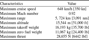

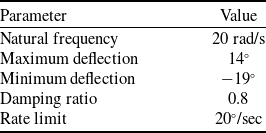
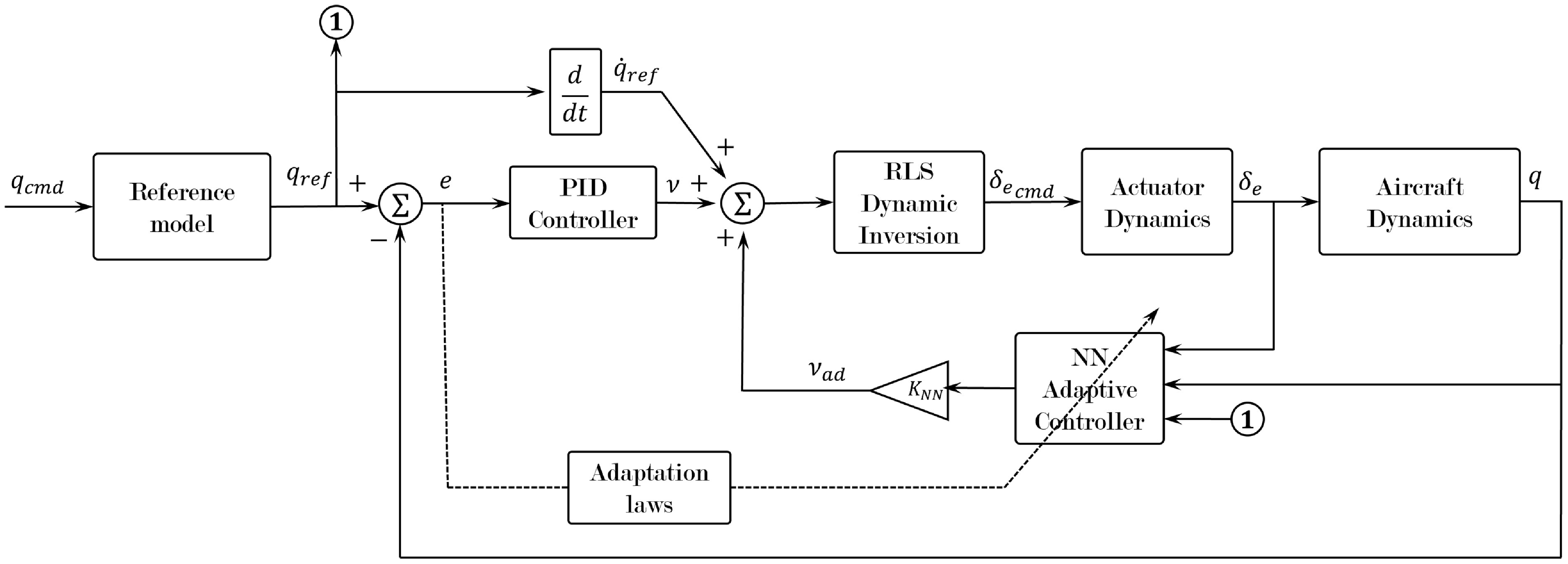
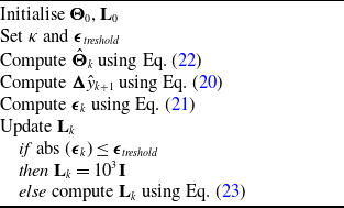
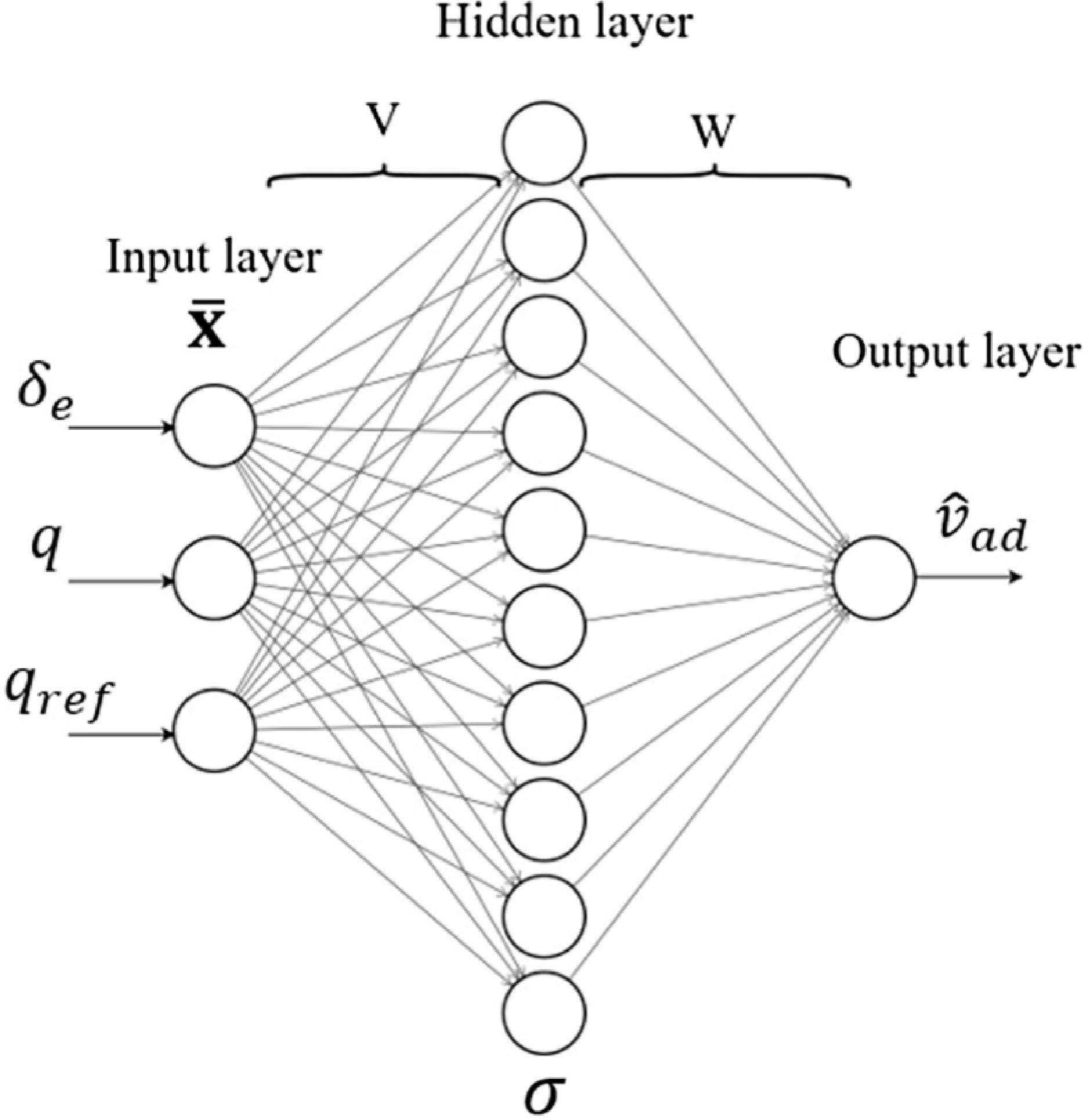
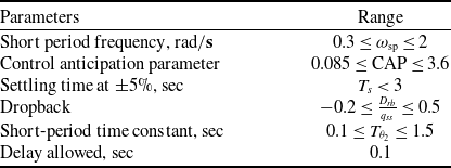
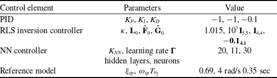
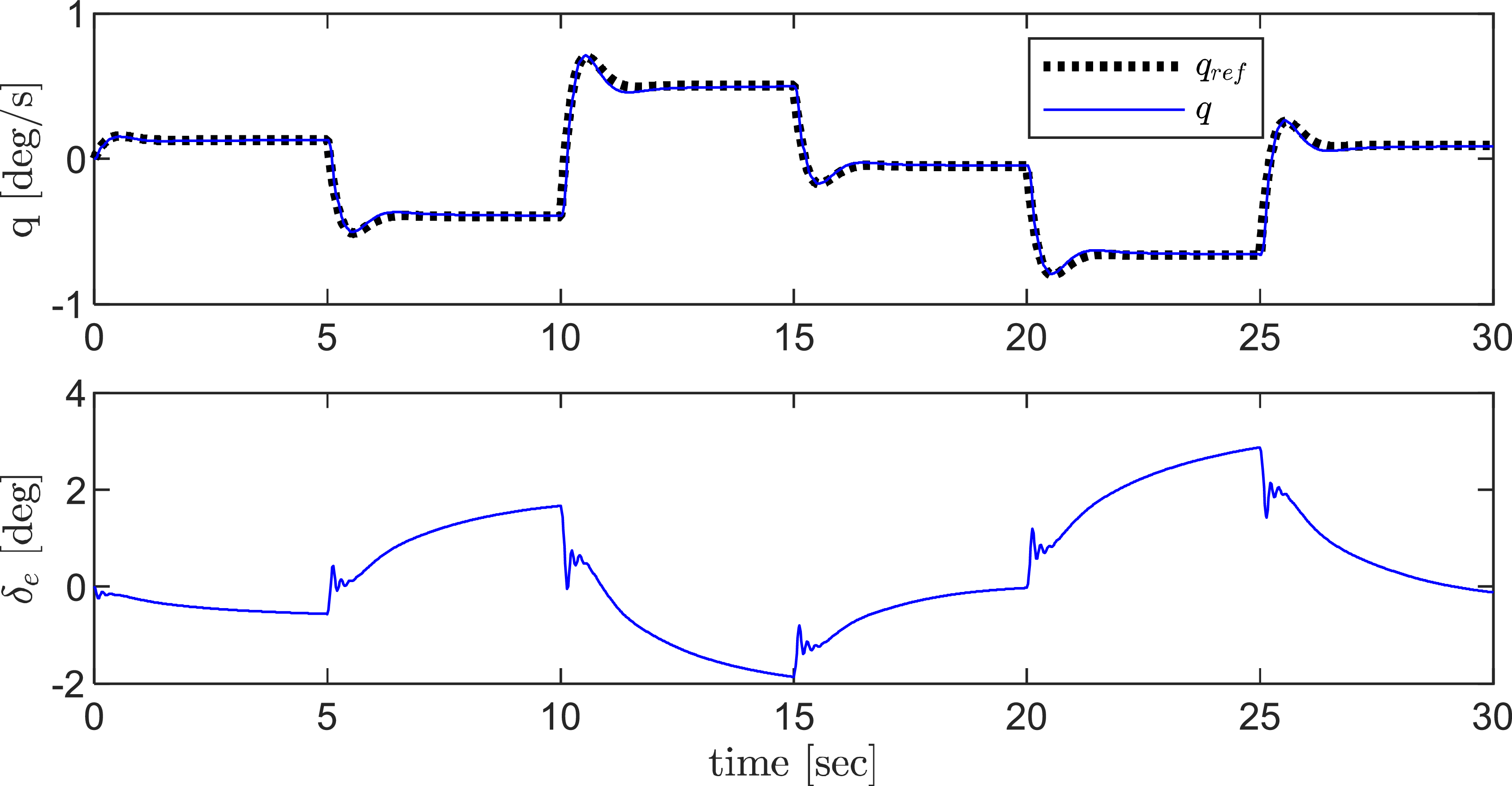
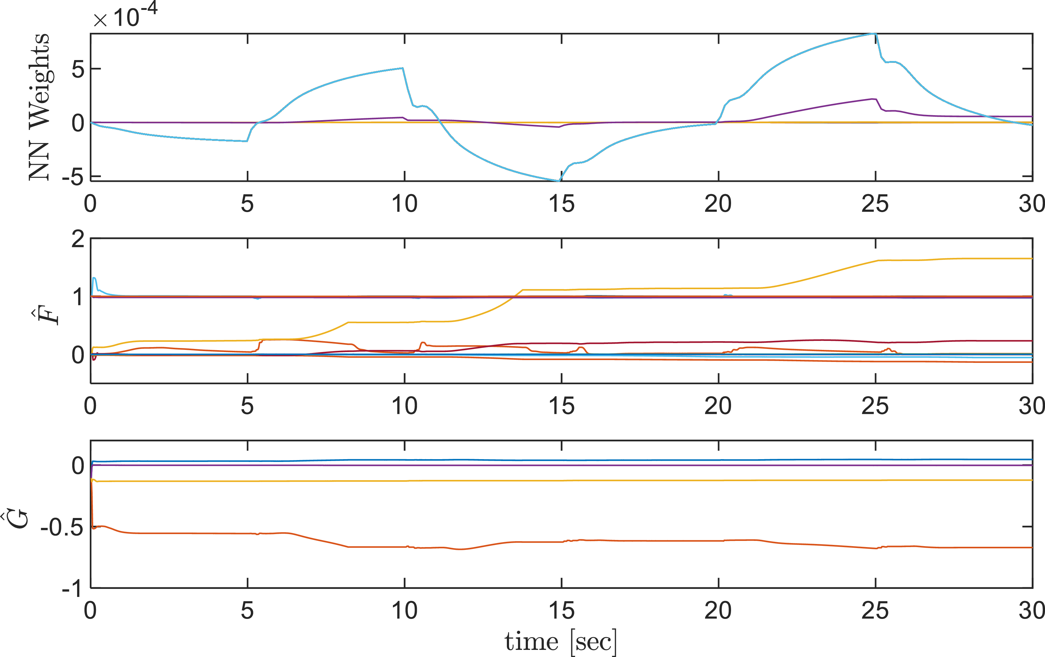


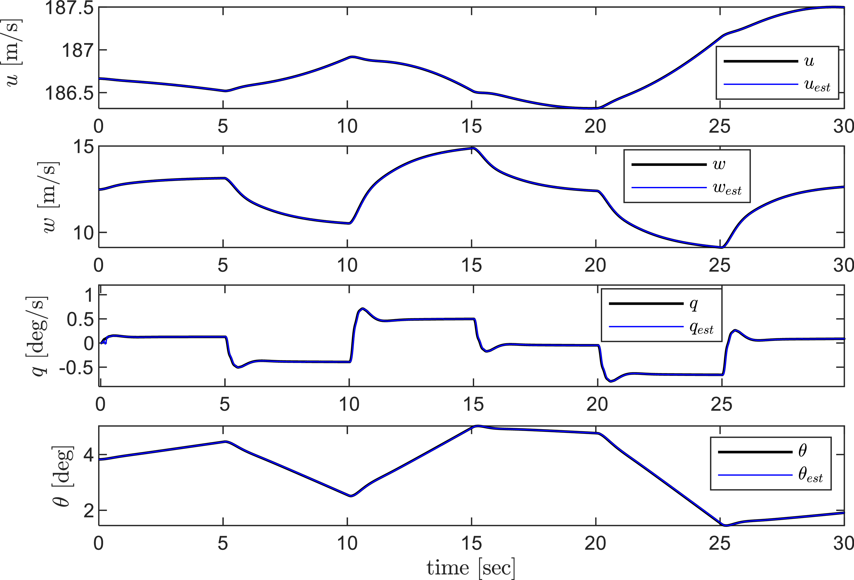
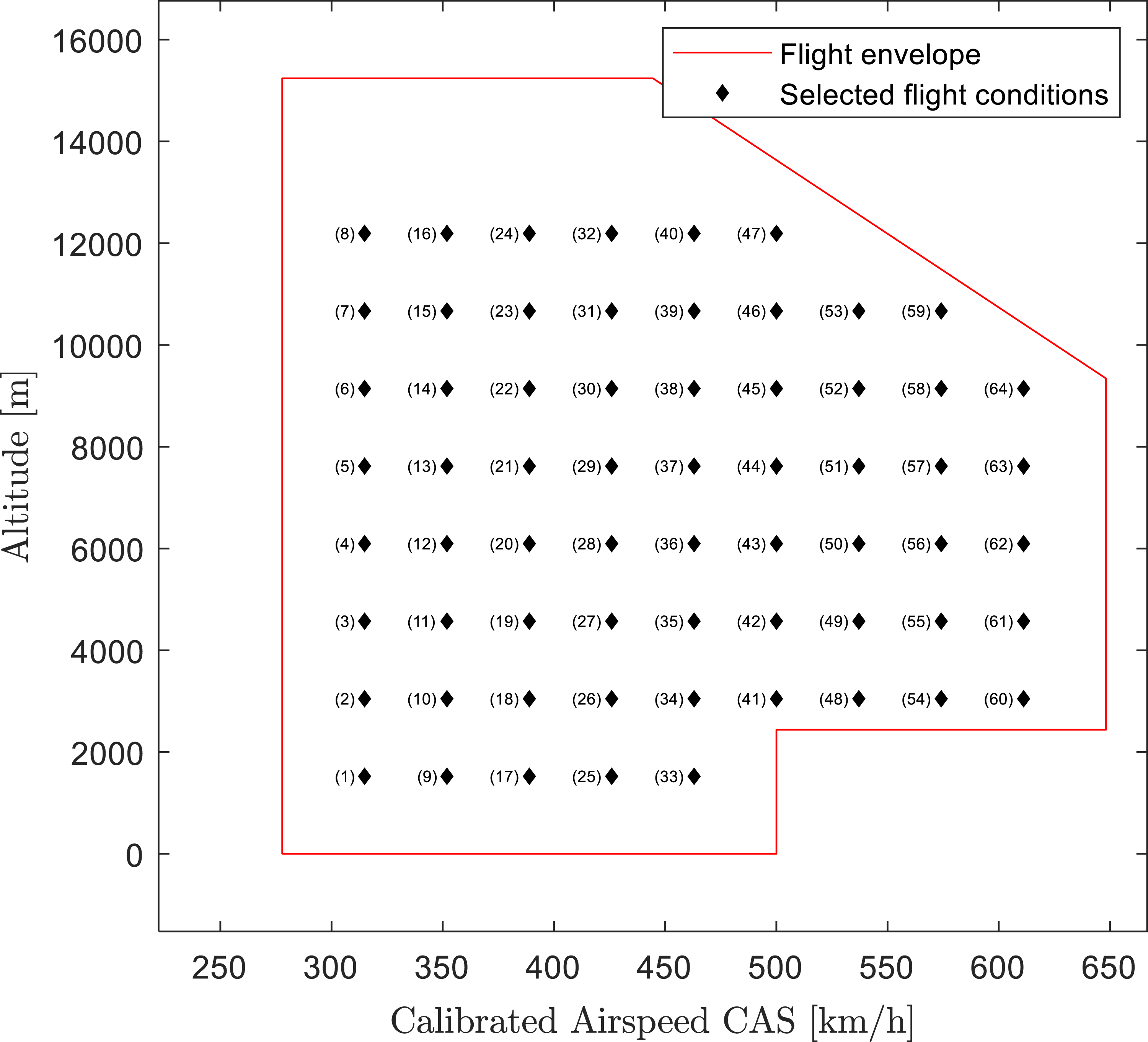


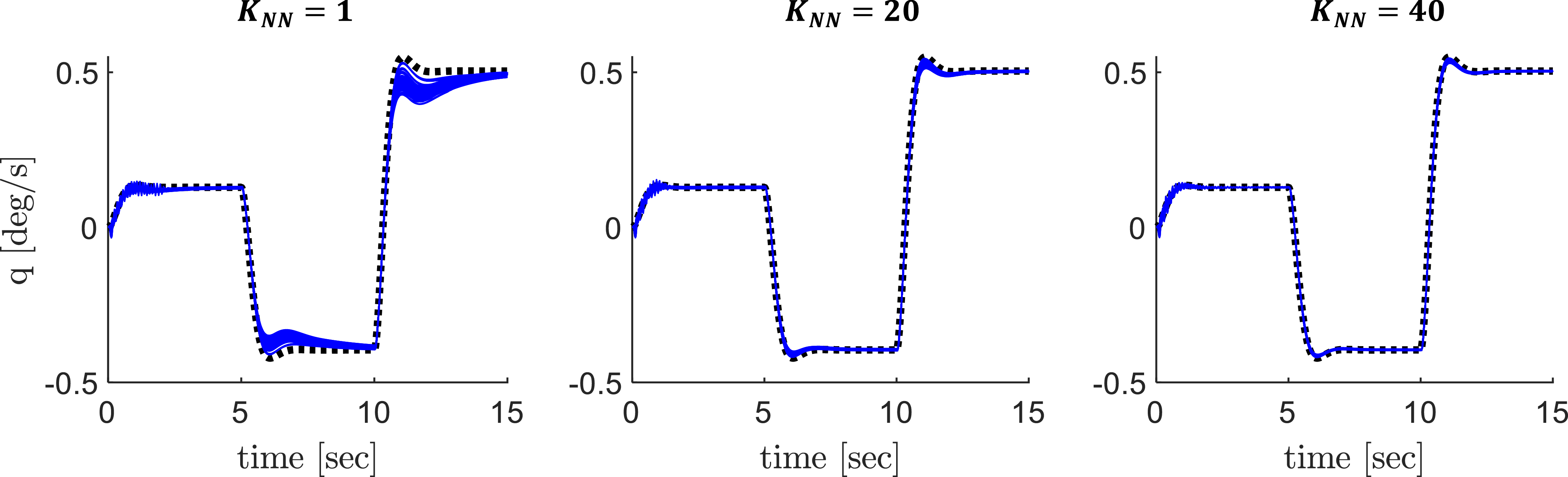


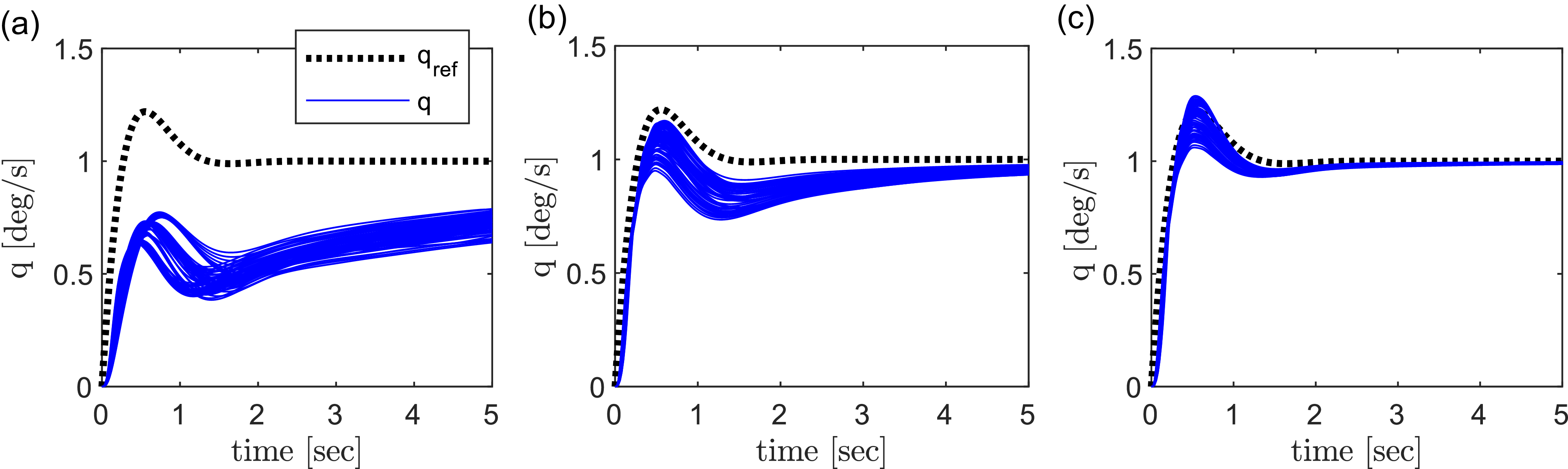
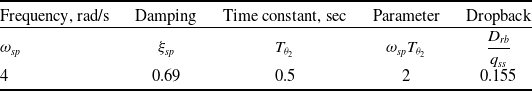
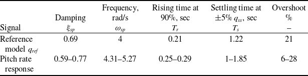


 Open access