


Impact Statement
Free-standing bodies like museum exhibits or large bridge piers can experience rocking motion when subjected to earthquakes. This response is notoriously difficult to predict given the hard nonlinearities arising from the multiple impacts and the response dependency on the initial conditions. The models presented in this article combine convolutional neural networks with the known rocking dynamics into a physics-informed data-driven framework that is able to predict the full history of the seismic response of rocking bodies with high accuracy provided the body does not overturn.
1. Introduction
For many years, the dynamics of rocking objects have captivated the attention of the scientific community, in part because it is a phenomenon that is frequently seen. A wide variety of structures engage in an uplifting response when faced with powerful dynamic actions (earthquakes, blasts, etc.) whose temporal evolution is infamously challenging to forecast and predict. From small but invaluable museum exhibits to substantial bridge piers or wind turbine towers, a wide variety of structures at all scales demonstrate this fundamental dynamic behavior. The underlying process of rocking motion has been demonstrated to be extremely complicated, sensitive to initial conditions, hence history-dependent, and by no means well understood, despite the apparently intuitive nature of the rocking motion (Ma, Reference Ma2010).
On the other hand, rocking structures are capable of uplifting and sustaining a strong nonlinear motion, while limiting the development of base moments since they are not fixed to the foundation or the ground (Thiers-Moggia and Málaga-Chuquitaype, Reference Thiers-Moggia and Málaga-Chuquitaype2021). It has been proposed that this uplift can act as a sort of rocking isolation for both bridges and buildings (Bachmann et al., Reference Bachmann, Strand, Vassiliou, Broccardo and Stojadinovic2019; Thiers-Moggia and Málaga-Chuquitaype, Reference Thiers-Moggia and Málaga-Chuquitaype2020; Vassiliou et al., Reference Vassiliou, Cengiz, Dietz, Dihoru, Broccardo, Mylonakis, Sextos and Stojadinovic2021). However, until recently it was been believed that analytical or numerical models can not accurately predict the rocking motion, as many efforts faced frequent failure in the recreation of experimental data (ElGawady et al., Reference ElGawady, Ma, Butterworth and Ingham2011; Kalliontzis and Sritharan, Reference Kalliontzis and Sritharan2018).
The rigid block rocking response is sensitive to defects in the supporting surfaces, as well as variations in initial conditions (Bachmann et al., Reference Bachmann, Strand, Vassiliou, Broccardo and Stojadinović2018). This makes it hard to precisely replicate the output of one experiment, suggesting that the seismic rocking motion of a rigid block is chaotic, to the extent that slight instabilities can result in vastly varied outcomes for a single excitation. The rigid rocking block numerical model most widely used today (Housner, Reference Housner1963) is deterministic, and the predicted seismic rocking response to a known support motion is susceptible to modeling assumptions, especially those regarding energy losses during ongoing impacts. Such sensitivity of rocking models discourages structural engineers from adopting rocking as an approach to modify earthquake response (Deng et al., Reference Deng, Kutter and Kunnath2012). It seems unfeasible to predict with sufficient certainty the seismic rocking response of blocks to a given ground excitation based on the results of a single experiment.
In this article, we follow the widespread assumption of planar rocking under unidirectional ground motion (Bachmann et al., Reference Bachmann, Vassiliou and Stojadinovic2021; Pan and Málaga-Chuquitaype, Reference Pan and Málaga-Chuquitaype2020; Reggiani Manzo and Vassiliou, Reference Reggiani Manzo and Vassiliou2021). Lachanas et al. (Reference Lachanas, Vamvatsikos and Vassiliou2022) found that the vertical ground motion component can exhibit a variable and sometimes significant impact on the rocking response which can be both detrimental and beneficial to the structural response; however, when considering a large dataset of records, this influence tends to become statistically insignificant. This also reflects the small number of studies to date that deal with the rocking of three-dimensional rigid bodies (Chatzis and Smyth, Reference Chatzis and Smyth2012). However, it is worth noting that two-dimensional models can represent the response of several practical applications such as planar wall elements and bridge piers with a relatively long length-to-thickness ratio (Thiers-Moggia and Málaga-Chuquitaype, Reference Thiers-Moggia and Málaga-Chuquitaype2020; Reggiani Manzo and Vassiliou, Reference Reggiani Manzo and Vassiliou2021). Besides, our approach and conclusions are applicable to rigid bodies with a vertical axis of symmetry and uniform density and can be extended to base-isolated rigid blocks (Pellecchia et al., Reference Pellecchia, Lo Feudo, Vaiana, Dion and Rosati2022).
Recently, the advancements in sensing and computational technologies have offered a major incentive for a wider adoption of structural health monitoring. The primary existing approaches concentrate on collecting structural elements and updating models from observed data. For example, the Bayesian probabilistic approach in model class selection (Vanik et al., Reference Vanik, Beck and Au2000; Beck and Yuen, Reference Beck and Yuen2004; Huang and Schröder, Reference Huang and Schröder2021), seismic interferometry in structural damage detection (Todorovska, Reference Todorovska2009; Sen et al., Reference Sen, Long, Sun, Campman and Buyukozturk2021; Uzun et al., Reference Uzun, Sun, Smit and Buyukozturk2021; García-Macías and Ubertini, Reference García-Macías and Ubertini2022) and Kalman filtering in dynamic force identification (Liu and Shepard, Reference Liu and Shepard2005; Lourens et al., Reference Lourens, Reynders, De Roeck, Degrande and Lombaert2012; Khodabandeloo and Jo, Reference Khodabandeloo and Jo2015; Naets et al., Reference Naets, Cuadrado and Desmet2015). However, it remains difficult to properly employ sensing data for modeling and predicting rocking responses under ground excitation, something to which this article aims to contribute.
1.1. Brief literature review
The seismic response of rigid rocking blocks is a highly non-linear phenomenon of difficult prediction due to its negative post-uplift stiffness and related impact phenomena (Bachmann et al., Reference Bachmann, Vassiliou and Stojadinovic2021; Reggiani Manzo and Vassiliou, Reference Reggiani Manzo and Vassiliou2021). Under strong base-shaking, slender blocks and tall rigid objects and structures may enter a rocking motion that occasionally results in overturning.
Conventional methods for predicting the seismic response of a structure make use of sensing data, such as identification-based approaches and analytical techniques (Zhang et al., Reference Zhang, Liu and Sun2020). In recent years, nonlinear response-history analysis has gained the community’s favor given its relatively precise quantification of structural responses, especially in terms of displacement histories whose peaks are strongly correlated with the damage condition of structural elements. Typically, the response history is estimated using numerical time-stepping methods in conjunction with finite-element (FE) modeling. Model updating can minimize the differences between the field sensed response of the actual structure and the reproduced response of the parameterized FE model. Model updating has been widely researched and employed to forecast the non-linear structural seismic response to known incoming inputs (Brownjohn and Xia, Reference Brownjohn and Xia2000; Sun and Betti, Reference Sun and Betti2015). However, since the number of parameters requiring updating is usually large and given the restricted availability of high-quality sensing data, these techniques still necessitate significant computing effort for updating FE models with high accuracy. And although low-fidelity models are more computationally efficient, it is difficult to maintain accuracy in the presence of uncertainties, particularly when modeling hard nonlinear responses like rocking.
Recent attention has concentrated on the application of artificial intelligence (AI) to the prediction of the seismic response of various structures. In this regard, AI has demonstrated its potential as an effective response modeling tool for a range of dynamic problems (Chen and Billings, Reference Chen and Billings1992; Chen and Chen, Reference Chen and Chen1993; Zhang et al., Reference Zhang, Sato and Iai2007). Within the field of structural dynamics, Neural Networks are one of the most prominent AI algorithms currently used. Over time, it has been conclusively established that neural networks can surpass alternative algorithms in terms of precision and speed. Convolutional neural network (CNN), recurrent neural networks (RNNs), AutoEncoders, and the like are gradually becoming the preferred tool of data scientists. As the present computer graphics cards are specifically built for parallel computing, deep learning–artificial neural networks (ANNs) are regarded as an effective and robust computational method for addressing difficult problems. The conventional multilayer perceptron (MLP) ANN algorithm has been used for modeling seismic responses of buildings throughout the previous decade, and many of them have started to incorporate the physics of the problem into their schemes of training.
Wu and Jahanshahi (Reference Wu and Jahanshahi2019) developed a CNN to identify and predict the dynamic response of a nonlinear single-degree-of-freedom (SDOF) system and a linear SDOF system, both with fixed bases. As a result of the convolution layers acting as filters, the suggested CNN method was more resistant to noisy input. Therefore, the developed CNN was suitable for predicting the dynamic response of an actual conventional fixed-base structure. Although the standard MLP ANNs model was more computationally efficient, difficulties subsisted in attaching a physical meaning to the model. The CNN, on the other hand, offered greater interpretability making it preferable to the typical MLP method.
Yu et al. (Reference Yu, Yao and Liu2020) proposed a unique physics-guided machine-learning technique for structural dynamics modeling based on RNN and MLP. In addition, this method also integrated the underlying knowledge of structural dynamics into a data-driven machine-learning framework to guide and train the model for prediction. The proposed physics-guided RNNs successfully predicted the dynamic response and showed successful generalization ability even under partially unknown physics.
Zhang et al. (Reference Zhang, Liu and Sun2020) presented a novel physics-guided convolutional neural network (PhyCNNs) for modeling the seismic response of structures by developing a data-driven surrogate. The performance of the proposed approach was validated both numerically and experimentally with only limited datasets from simulations and real sensing measurements. Their results proved that the PhyCNN framework is computationally efficient for modeling the seismic response. It was suggested that the proposed algorithm was basic and could be easily scalable to other structures subjected to other kinds of hazards.
All the studies mentioned above have dealt with fixed-base structures. By contrast, not many studies have examined the use of data-driven methods for the response prediction of uplifting structures that engage in rocking motion. In fact, many researchers believe that the rigid rocking block is a chaotic system for which minor changes in its governing parameters (block characteristics, initial conditions, or base excitation) can lead to drastically divergent results (Bachmann et al., Reference Bachmann, Strand, Vassiliou, Broccardo and Stojadinović2018). The experiments conducted by Vassiliou et al. (Reference Vassiliou, Truniger and Stojadinović2015) and Kalliontzis et al. (Reference Kalliontzis, Sritharan and Schultz2016) to confirm Housner’s rigid rocking model (Housner, Reference Housner1963) indicated that, given the modeling uncertainties, particularly those relative to impact, estimating the seismic response history of a certain rocking block to a specific ground excitation is hard.
In this context, Pan et al.’s (Reference Pan, Wen and Yang2021) work showed that by implementing neural networks the computational time required to estimate the rocking response of a rigid block can be significantly reduced compared to the use of FE models, especially when the Graphical Processing Unit’s acceleration is enabled. The networks trained by Pan et al. (Reference Pan, Wen and Yang2021) were able to construct the rocking spectrum of structures more effectively than FE runs; however, a large database was required to complete a significant number of dynamic response-history analyses.
More recently, Achmet et al. (Reference Achmet, Diamantopoulos and Fragiadakis2023) proposed a ML-based tool for the rapid assessment of damage to rocking systems using the k-nearest neighbor (k-NN) algorithm and support vector machines (SVMs). This is a second attempt to effectively use machine-learning algorithms to assess the seismic performance of rigid bodies under ground motion. The study concluded that ML algorithms are promising for the case of rocking structures. Although some loss of precision was documented when dealing with real ground-motion records.
To the authors’ knowledge, the two studies mentioned above are the only ones to attempt to model the structural response of rocking systems with AI tools. Besides, advanced deep learning models like ANNs, RNNs, and CNNs as discussed above, have not been applied to the rocking problem in combination with embedded physical relationships. It should be noted that ANN alone is incapable of capturing sequential information in input data, which is necessary for processing the data containing time series typical of seismic responses. The other two deep learning architectures—RNN and CNN can overcome this limitation in conventional MLP. However, RNNs require a large number of time steps in processing and are susceptible to the vanishing and exploding gradient problem. In this article, we present a first attempt to apply advanced deep learning tools in combination with physics-informed approaches to solve full rocking response estimations.
1.2. Research aims and objectives
In this article, a physics-informed convolutional neural network (PICNN) is proposed for simulating the rocking response of free-standing rigid blocks subjected to ground excitation. This newly developed tool intends to solve the limitations of mechanics-based numerical modeling on the one hand, and solely data-driven modeling of the rocking response on the other. This is done by adding a physic-based component to a data-driven CNN to achieve a more accurate estimation of the rocking response-histories of ideally rigid blocks in a hybrid data-driven way.
Inspired by previous studies that used PICNNs for the seismic response prediction of fixed-based structures, e.g., Zhang et al. (Reference Zhang, Liu and Sun2020), this study modifies and extends PICNNs reach to the more difficult task of predicting rocking behavior. Likewise, in comparison with other purely data-driven methodologies proposed for the assessment of rigid rocking motion, e.g., Achmet et al.’s (Reference Achmet, Diamantopoulos and Fragiadakis2023), the PICNN framework proposed here aims to achieve a higher computational efficiency with less training time and requiring fewer labeled samples. Besides, the newly proposed models better capture the complex and hard non-linear relationships in the time-series data; reduce the need for manual feature engineering, and explicitly incorporate the constraints of the equation of motion into the training process.
The basic idea is to first make the known physics accessible to the deep-learning framework by defining the physics loss function. Then, the PICNNs are trained by creating and using seismic datasets with the aid of a widely used numerical model of the rigid block rocking response. It should be noted, however, that the door is open for the use of experimental data when such dataset becomes available. Finally, the trained PICNN model is validated and observations are made on its performance.
The article is organized as follows. Section 2 presents the dynamics of rocking motion and introduces the development of the training datasets from numerical analysis. Section 3 presents the architecture of the PICNN framework for rocking structural seismic response. Then, the data analysis is presented including numerical validation of the deep PICNN framework through examples containing only the ground acceleration measurements. Two model cases will be examined, Model 1 which uses available input measurements of angular displacement and velocity, while Model 2 only relies on available measurements of angular acceleration. For each model case, an optimization study will be conducted to determine its performance and limitations. Section 5 presents a discussion on the performance of the PICNN framework for seismic rocking response based on the results and analysis performed in the previous sections, followed by an analysis of the limitations of this study and recommendations for further work. Finally, the conclusions of this study are summarized in Section 6.
2. The seismic response of free-standing rigid rocking blocks
This article deals with the rocking response and stability of rigid blocks subjected to a horizontal ground excitation $ {\ddot{u}}_g $
. The schematics of the problem are shown in Figure 1. The rigid object under consideration is a single slender block of size
$ {\ddot{u}}_g $
. The schematics of the problem are shown in Figure 1. The rigid object under consideration is a single slender block of size $ R $
and slenderness
$ R $
and slenderness $ \alpha $
. It is assumed that the rigid block is placed on a surface where the coefficient of friction is large; therefore no sliding is observed between the block and the base and the block engages in rotational motion around the pivot points
$ \alpha $
. It is assumed that the rigid block is placed on a surface where the coefficient of friction is large; therefore no sliding is observed between the block and the base and the block engages in rotational motion around the pivot points $ O $
or
$ O $
or $ {O}^{\prime } $
. The size of the rigid block is defined in equation (1) and its slenderness is defined in equation (2):
$ {O}^{\prime } $
. The size of the rigid block is defined in equation (1) and its slenderness is defined in equation (2):
 $$ R=\sqrt{H^2+{B}^2}, $$
 $$ \alpha =a\tan \left(\frac{b}{h}\right), $$
where $ R $
is the block semi-diagonal (i.e., the radial distance from the center of rotation
$ R $
is the block semi-diagonal (i.e., the radial distance from the center of rotation $ O $
to the center of gravity),
$ O $
to the center of gravity), $ H $
is the location of the center of gravity above the base of the block and
$ H $
is the location of the center of gravity above the base of the block and $ B $
is the distance of the center of gravity from the side,
$ B $
is the distance of the center of gravity from the side, $ \alpha $
is the block slenderness (i.e.,
$ \alpha $
is the block slenderness (i.e., $ \alpha $
is the angle the block semi-diagonal made with the vertical when the block is at rest, in [rad]), and the angle
$ \alpha $
is the angle the block semi-diagonal made with the vertical when the block is at rest, in [rad]), and the angle $ \theta $
quantifies the block’s rotation. In particular, the case study considered in this article, deals with a block semi-diagonal
$ \theta $
quantifies the block’s rotation. In particular, the case study considered in this article, deals with a block semi-diagonal $ R=9 $
m and a block slenderness
$ R=9 $
m and a block slenderness $ \alpha =0.06 $
rad, which is representative of a rigid bridge pier (Thiers-Moggia and Málaga-Chuquitaype, Reference Thiers-Moggia and Málaga-Chuquitaype2020).
$ \alpha =0.06 $
rad, which is representative of a rigid bridge pier (Thiers-Moggia and Málaga-Chuquitaype, Reference Thiers-Moggia and Málaga-Chuquitaype2020).
Geometric characteristics of the rigid block model.

The rigid block will uplift and start to rock when the overturning moment is greater than the restoring moment as a result of its self-weight. The corresponding mathematical expression is shown by
 $$ {\ddot{u}}_g\ge g\tan \alpha, $$
where $ g $
is the acceleration of gravity. The equation of motion for the rocking block, assuming that no sliding or bouncing occurs during impact, can be described based on Housner’s (Reference Housner1963) model and is expressed as follows (Vassiliou et al., Reference Vassiliou, Truniger and Stojadinović2015):
$ g $
is the acceleration of gravity. The equation of motion for the rocking block, assuming that no sliding or bouncing occurs during impact, can be described based on Housner’s (Reference Housner1963) model and is expressed as follows (Vassiliou et al., Reference Vassiliou, Truniger and Stojadinović2015):
 $$ {I}_o\ddot{\theta}(t)+ mg\;R\sin\;\left[-\alpha -\theta (t)\right]=-m{\ddot{u}}_g(t)R\cos\;\left[-\alpha -\theta (t)\right],\hskip0.6em \theta (t)<0, $$
 $$ {I}_o\ddot{\theta}(t)+ mg\;R\sin\;\left[\alpha -\theta (t)\right]=-m{\ddot{u}}_g(t)R\cos\;\left[\alpha -\theta (t)\right],\hskip0.6em \theta (t)>0, $$
where for a rectangular block $ {I}_o=\left(4/3\right){mR}^2 $
; therefore, equations (4) and (5) can be rewritten as follows:
$ {I}_o=\left(4/3\right){mR}^2 $
; therefore, equations (4) and (5) can be rewritten as follows:
 $$ \ddot{\theta}(t)+{p}^2\sin\;\left[\alpha sgn\left(\theta (t)\right)-\theta (t)\right]-\frac{{\ddot{u}}_g}{g}\cos\;\left[\alpha sgn\left(\theta (t)\right)-\theta (t)\right]=0, $$
where $ p $
is the quantity that characterizes the dynamic properties of the block and
$ p $
is the quantity that characterizes the dynamic properties of the block and $ p $
represents the in-plane pendulum frequency of the same block dangling from its pivot point. For a rectangular block
$ p $
represents the in-plane pendulum frequency of the same block dangling from its pivot point. For a rectangular block $ p=\sqrt{3g/4R} $
. The case study used in this article has a
$ p=\sqrt{3g/4R} $
. The case study used in this article has a $ p=0.904\hskip0.4em \mathrm{rad}/\mathrm{s} $
.
$ p=0.904\hskip0.4em \mathrm{rad}/\mathrm{s} $
.
An important feature of the rocking response is the impact phenomenon that occurs once the angle of rotation $ \theta $
reverses, losing some of its kinetic energy. This energy loss is expressed in terms of a coefficient of restitution
$ \theta $
reverses, losing some of its kinetic energy. This energy loss is expressed in terms of a coefficient of restitution $ {V}_{\mathrm{loss}} $
that relates the angular velocity before impact
$ {V}_{\mathrm{loss}} $
that relates the angular velocity before impact $ {\dot{\theta}}_1 $
to the post-impact angular velocity
$ {\dot{\theta}}_1 $
to the post-impact angular velocity $ {\dot{\theta}}_2 $
in the following way:
$ {\dot{\theta}}_2 $
in the following way:
 $$ {\dot{\theta}}_2={V}_{\mathrm{loss}}{\dot{\theta}}_1. $$
The widely used Housner’s model (Housner, Reference Housner1963) implies an equality of the moment of momentum before and after impact that results in a coefficient of restitution that depends only on the geometry and mass of the block. In this article, we consider $ {V}_{\mathrm{loss}} $
to be an independent parameter of the rocking problem and assume two values of it (0.9 and 0.5) to examine its influence on the accuracy of the proposed PICNN model.
$ {V}_{\mathrm{loss}} $
to be an independent parameter of the rocking problem and assume two values of it (0.9 and 0.5) to examine its influence on the accuracy of the proposed PICNN model.
It is also possible that, depending on the signature of the base acceleration, the rigid block will overturn before or after impact. In this study, over-turning is defined by computing the full rotation history of the block to determine whether the rigid block topples or not when subjected to a particular ground motion.
The aforementioned equations were scripted and solved in MATLAB (version 2023(b)) to simulate the two-dimensional seismic response of a rigid block. Moreover, a selection of ground motion records taken from the PEER Ground Motion database (Chiou et al., Reference Chiou, Darragh, Gregor and Silva2008) was used. This ground-motion database comprises a total of 1656 samples (i.e., independent seismic record sequences) and the corresponding number of response histories were generated. For each seismic simulation, a time period of 60 seconds was selected with time steps of 0.05 seconds resulting in 1200 data points per record.
Table 1 presents a summary of the database of records used as input to generate the rocking responses in this article. Mean values as well as representative peak characteristics of the acceleration records are presented for the whole NGA database used as well as a sub-set of stronger records selected on the basis of their amplitude and duration to have a larger energetic content delivered in a shorter period of time as will be described later in the article.
Main characteristics of the ground-motion record sets used

In deep learning, the selection of the training datasets has a crucial function. In general, the data would be randomly divided into training, validation, and prediction sets, in the ratios of 70%, 15%, and 15%, respectively. This approach to data partition was also followed in this study. Moreover, since the whole dataset is expected to be influenced by the ground-motion characteristics of the input acceleration record set, any random divisions of the data would impact significantly the ability of the generalized trained model. Therefore, a K-means clustering approach was followed for data clustering. K-means clustering, a type of unsupervised learning, has the advantages of easy implementation; and with a large number of variables, it can be computationally fast and guarantees convergence (Yuan and Yang, Reference Yuan and Yang2019).
The performance of the PICNN for predicting rocking behavior will be assessed through numerical validation assuming that histories of rotation $ \theta $
, angular velocity
$ \theta $
, angular velocity $ \dot{\theta} $
, and accelerations
$ \dot{\theta} $
, and accelerations $ \ddot{\theta} $
are available for training. These histories are available from the MATLAB simulations described above but can be potentially obtained from measurements. In addition, several optimization studies will be conducted to investigate the performance of the proposed PICNN model when predicting the rocking response for accessing real field measurements in applications: (i) including overturning cases or not including overturning; or (ii) restricting or not restricting the range of ground motions used for input training. To this end, comparative analysis of the predicted measurements from the deep PICNN and the reference measures from the numerical model will be presented in terms of response-history comparisons and statistical analysis techniques to establish a quantitative measure of the performance of the PICNN in estimating the rocking response under earthquake excitations. This will indicate whether the deep PICNN is adequate or not for assessing the rocking response of the rigid block subjected earthquake motion. Before introducing the performance metrics employed, the following section will present the PICNN framework used.
$ \ddot{\theta} $
are available for training. These histories are available from the MATLAB simulations described above but can be potentially obtained from measurements. In addition, several optimization studies will be conducted to investigate the performance of the proposed PICNN model when predicting the rocking response for accessing real field measurements in applications: (i) including overturning cases or not including overturning; or (ii) restricting or not restricting the range of ground motions used for input training. To this end, comparative analysis of the predicted measurements from the deep PICNN and the reference measures from the numerical model will be presented in terms of response-history comparisons and statistical analysis techniques to establish a quantitative measure of the performance of the PICNN in estimating the rocking response under earthquake excitations. This will indicate whether the deep PICNN is adequate or not for assessing the rocking response of the rigid block subjected earthquake motion. Before introducing the performance metrics employed, the following section will present the PICNN framework used.
3. Physics-informed CNN framework
This section presents the architecture of the PICNN to estimate the seismic response of rocking structures. Two model cases are introduced and discussed with emphasis on the definition of their loss functions.
As discussed in Section 1.1, there appears to be a consensus that neural networks are an effective technique for solving problems like classification and regression (Bharath and Reza, Reference Bharath and Reza2018). CNN (or ConvNet) is a class of ANN, used most frequently to examine visual images (Ciresan et al., Reference Ciresan, Meier, Masci, Gambardella and Schmidhuber2011; Valueva et al., Reference Valueva, Nagornov, Lyakhov, Valuev and Chervyakov2020) with widespread applications in image classification, image segmentation, medical image analysis and brain–computer interfaces (Avilov et al., Reference Avilov, Rimbert, Popov and Bougrain2020). Deep neural networks have traditionally been trained using data alone. However, by including physical restrictions (e.g., the governing laws of dynamics) throughout the training step, the resilience of learning from the data may be improved even further.
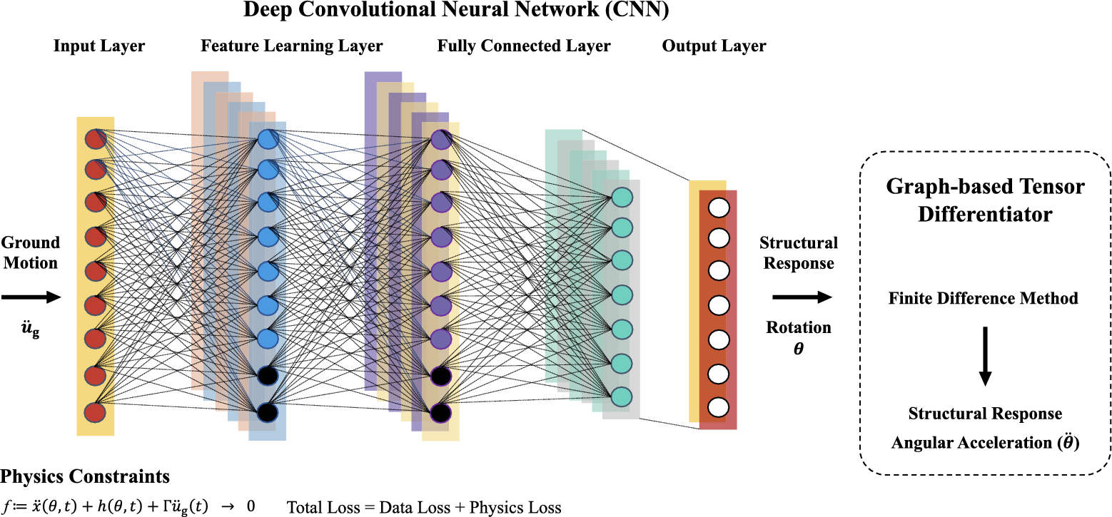
A four-layer PICNN is proposed herein for the analysis of response series as shown in Figure 2. The four layers comprise a feature learning layer, a fully-connected layer, and input and output layers. Also, one graph-based tensor differentiator is used. In this study, dropout layers are additionally implemented to avoid complex modifications to the training data (Srivastava et al., Reference Srivastava, Hinton, Krizhevsky, Sutskever and Salakhutdinov2014; Zhang et al., Reference Zhang, Liu and Sun2020).
The architecture of physics-informed convolutional neural network (PICNN). The inputs are ground motion ( $ {\overset{}{u}}_g $
), and the outputs are state space variables: rotation (
$ {\overset{}{u}}_g $
), and the outputs are state space variables: rotation ( $ \theta $
), rotational velocity (
$ \theta $
), rotational velocity ( $ \dot{\theta} $
). The derivatives of the outputs from the tensor differentiator are angular velocity (
$ \dot{\theta} $
). The derivatives of the outputs from the tensor differentiator are angular velocity ( $ {\theta}_t $
), acceleration (
$ {\theta}_t $
), acceleration ( $ {\dot{\theta}}_t $
).
$ {\dot{\theta}}_t $
).
In general, for the prediction of seismic responses, the inputs are the ground motion records (real or artificial), and the outputs are histories of structural response parameters like structural displacement $ x\left(\theta, t\right) $
or structural velocity
$ x\left(\theta, t\right) $
or structural velocity $ \dot{x}\left(\theta, t\right) $
. It should be noted that the velocities
$ \dot{x}\left(\theta, t\right) $
. It should be noted that the velocities $ \dot{x}\left(\theta, t\right) $
are worked out through the tensor differentiator by unitizing the finite difference method (FDM). The combined loss is the sum of the loss of measurement data and the loss resulting from the physics used to simulate the interdependence of the output characteristics. Different to the general CNN, the input and output in the deep PICNN framework are both time sequences.
$ \dot{x}\left(\theta, t\right) $
are worked out through the tensor differentiator by unitizing the finite difference method (FDM). The combined loss is the sum of the loss of measurement data and the loss resulting from the physics used to simulate the interdependence of the output characteristics. Different to the general CNN, the input and output in the deep PICNN framework are both time sequences.
To fit better more conventional expressions used in the PICNN modeling of dynamic systems, the governing equation of motion for a rocking body can be expressed as follows:
 $$ f:= \ddot{x}\left(\theta, t\right)+h\left(\theta, t\right)+\Gamma {\ddot{u}}_g(t)\hskip0.36em \to 0, $$
where $ \ddot{x}\left(\theta, t\right) $
is the acceleration relative to the ground,
$ \ddot{x}\left(\theta, t\right) $
is the acceleration relative to the ground, $ h\left(\theta, t\right) $
is the generalized term,
$ h\left(\theta, t\right) $
is the generalized term, $ {\ddot{u}}_g $
is the ground motion, and
$ {\ddot{u}}_g $
is the ground motion, and $ \Gamma $
is the force distribution factor.
$ \Gamma $
is the force distribution factor.
A graph-based tensor differentiator is incorporated with the one-dimensional CNN in order to relate different physical parameters of varying temporal nature. The basic concept of the network is to give the ground acceleration as input (containing $ n $
test points with time series from
$ n $
test points with time series from $ {t}_1 $
to
$ {t}_1 $
to $ {t}_n $
), and then output the state space variables containing displacement
$ {t}_n $
), and then output the state space variables containing displacement $ x\left(\theta, t\right) $
, the velocity
$ x\left(\theta, t\right) $
, the velocity $ \dot{x}\left(\theta, t\right) $
. All the inputs and outputs are time-related and have the sample points from
$ \dot{x}\left(\theta, t\right) $
. All the inputs and outputs are time-related and have the sample points from $ {t}_1 $
to
$ {t}_1 $
to $ {t}_n $
. As detailed later the convolution operation, zero-padding is added to each convolution layer’s output sequence to guarantee the same input/output length.
$ {t}_n $
. As detailed later the convolution operation, zero-padding is added to each convolution layer’s output sequence to guarantee the same input/output length.
In addition to the input and output layers, the PICNN framework also includes several hidden layers named the feature learning layers and the fully connected layers (Lawrence et al., Reference Lawrence, Giles, Tsoi and Back1997; Lecun et al., Reference Lecun, Bengio and Hinton2015). A convolution layer, a nonlinear activation function, and a feature pooling layer are among them and compose the feature learning layer. The sets of sample points that pass through each layer will output a feature map, as the feature pooling layers are used to extract the characteristics from the input/output from the preceding layer.
In order to add the physics-informed component into the CNN framework, the outputs passed through the convolution layers will be further processed by a graph-based tensor differentiator based on the FDM to get its derivation $ \dot{\theta}(t) $
,
$ \dot{\theta}(t) $
, $ \ddot{\theta}(t) $
which works as the main variables in the physics loss function. In general, the simplest and the most common loss calculated for deep learning model uncertainty is the mean squared error (MSE). In this article, the weighted mean squared error (WMSE) is used to assign different weights to individual parameters based on significance in the overall optimization process. This approach enables PINNs to effectively handle imbalanced data, incorporate the physics of the problem, and account for data uncertainties, further achieve more accurate and robust results during the optimization process.
$ \ddot{\theta}(t) $
which works as the main variables in the physics loss function. In general, the simplest and the most common loss calculated for deep learning model uncertainty is the mean squared error (MSE). In this article, the weighted mean squared error (WMSE) is used to assign different weights to individual parameters based on significance in the overall optimization process. This approach enables PINNs to effectively handle imbalanced data, incorporate the physics of the problem, and account for data uncertainties, further achieve more accurate and robust results during the optimization process.
The fundamental idea of constructing the physics loss here is to make the network hyper-parameters (equation (9)) as optimal as possible so that the PICNN can comprehend the measurement data while also meeting the physical relationships of the governing equation of motion, as shown in equation (8):
 $$ \theta =\left\{{W}_{\theta },{b}_{\theta}\right\}, $$
where $ {W}_{\theta } $
is the weight parameter of the neural network and
$ {W}_{\theta } $
is the weight parameter of the neural network and $ {b}_{\theta } $
is the neural network bias parameter. For the total loss,
$ {b}_{\theta } $
is the neural network bias parameter. For the total loss, $ J\left(\theta \right) $
, which comprises data loss and physics loss, the definitions are shown below:
$ J\left(\theta \right) $
, which comprises data loss and physics loss, the definitions are shown below:
 $$ J\left(\theta \right)={J}_D\left(\theta \right)+{J}_P\left(\theta \right), $$
 $$ {J}_D\left(\theta \right)=\frac{1}{N}\sum \limits_{i=1}^N{\left({x}_i^p-{x}_i^m\right)}^2+\frac{1}{N}\sum \limits_{i=1}^N{\left({{\dot{x}}_i}^p-{{\dot{x}}_i}^m\right)}^2+\frac{1}{N}\sum \limits_{i=1}^N{\left({h}^p-{h}^m\right)}^2, $$
 $$ {J}_P\left(\theta \right)=\frac{1}{N}\sum \limits_{i=1}^N{\left({\dot{x}}^p-{x}_t^p\right)}^2+\frac{1}{N}\sum \limits_{i=1}^N{\left({\dot{x}}_t^p+{h}^p+\Gamma {\ddot{u}}_g\right)}^2, $$
where $ {J}_D\left(\theta \right) $
is the data measurements loss,
$ {J}_D\left(\theta \right) $
is the data measurements loss, $ {J}_P\left(\theta \right) $
is the physics loss defined to impose a restriction that can be used to simulate the interdependence of the output characteristics in the neural work framework;
$ {J}_P\left(\theta \right) $
is the physics loss defined to impose a restriction that can be used to simulate the interdependence of the output characteristics in the neural work framework; $ p $
and
$ p $
and $ m $
are superscripts denoting prediction and measurement.
$ m $
are superscripts denoting prediction and measurement.
The application of the standard neural network (for example, ANN and CNN) is limited in practice, due to the unavoidably huge numerical inaccuracies resulting from the integration of accelerations to displacements. This normal approach requires firstly the determination of the structural displacements based on the ground acceleration data, and then the training of a CNN model using the interpreted displacements. The PICNN embeds the physical relationships into its training; theoretically speaking, it would be able to accurately predict the block rotations (or related drifts) only based on the ground accelerations. In the following subsections, the features of the four different kinds of layers used will be detailed.
3.1. Convolution layer
The convolution layer is the foundation of the PICNN framework, and is an essential part of building the CNN. A convolutional layer works like an ordinary neural network in a hidden layer, it converts the input to an abstract representation. To execute computations between feed-in value and the hidden neurons, the convolutional layer employs a local connection rather than a whole connectivity. It uses at least one kernel to conduct a convolution between each region of input and the kernel as it slides over the input. The activation maps, which may be viewed as the outcome from the convolutional layer, store the findings including characteristics derived from several kernels. Every kernel can serve as a feature extractor individually and all neurons will share their weights. By convolving an input sequence throughout the full temporal space, the time dependence is recorded.
Typically, a nonlinear activation function (such as ReLu, tanh, etc.) is implemented to the values resulting from convolutional actions between the kernel and the input. Those values are recorded in the activation maps and will be eventually sent to the subsequent network layers. In this study, a RelU function was applied as defined in the following equation:
 $$ f(x)=\left\{\begin{array}{rrr}0& \mathrm{for}\hskip0.5em x<0& \\ {}x& \mathrm{for}\hskip0.5em x\ge 0& \end{array}\right.\hskip-0.5em . $$
3.2. Pooling layer
Pooling layers offer a method for downsampling feature maps by summarizing the existence of characteristics within patches of the characteristic mapping. Common pooling techniques include average pooling and max pooling, which summarize the average presence of a feature or the most active presence of a feature, respectively. Average Pooling Computes the mean value for each patch on the map. Maximum Pooling determines the largest value for each patch of a feature map. For the proposed PICNN framework, the pooling layer is restricted as the feature of downsampling is not wanted for solving regression problems involving time series like the one under consideration.
3.3. Fully-connected layer
A layer with full connectivity multiplies the feed-in value by a weight matrix and then adds a bias vector (Géron, Reference Géron2019). Normally, One or more fully connected layers come after the convolutional (downsampling) layers. As suggested by the name, all neurons in the completely connected layer are linked to all neurons in the layer underneath it. To solve the regression problem (time-series prediction) like the one presented in this study, a $ \mathrm{Tanh} $
function (nonlinear activation functions) is implemented within the fully-connected layers with the linear activation functions applied to the output layer (Zhang et al., Reference Zhang, Liu and Sun2020).
$ \mathrm{Tanh} $
function (nonlinear activation functions) is implemented within the fully-connected layers with the linear activation functions applied to the output layer (Zhang et al., Reference Zhang, Liu and Sun2020).
3.4. Dropout layer
A dropout layer is one of the most widely used regularization approaches for minimizing overfitting in deep learning models. When a model exhibits more accuracy on the training data but poorer accuracy on the test data or unknown data, this is known as overfitting. In the dropout approach, random neurons are deleted or excluded from hidden or visible layers. Normally, the dropout layer can be placed after each convolution layer or fully-connected layer. The input units are set to zero at random at each training step with the frequency of rate. Inputs that are not set to zero are multiplied by 1/(1 − rate) such that the sum of all inputs remains unchanged. The dropout rate in this study was set to 0.2 and placed before the fully-connected layers. Finally, to get the model trained in a local PC environment, the authors used a standard PC with 32 GB memory, 12th Gen Intel Core i7–12,700 CPU and an NVIDIA RTX A4500 video card.
3.5. Rotation-rotational velocity model: model 1
The first model developed will assume that measurements of all state variables ( $ \theta $
and
$ \theta $
and $ \dot{\theta} $
) are available for training. This condition is typical of datasets developed via numerical models, like the one described above. In this case, the loss function is defined as the sum of the data loss and physics loss, referring to equations (8)–(12), the equation of motion of the nonlinear rocking system, therefore, can be expressed as follows:
$ \dot{\theta} $
) are available for training. This condition is typical of datasets developed via numerical models, like the one described above. In this case, the loss function is defined as the sum of the data loss and physics loss, referring to equations (8)–(12), the equation of motion of the nonlinear rocking system, therefore, can be expressed as follows:
 $$ \ddot{\theta}(t)+\underset{h}{\underbrace{p^2\sin\;\left[\alpha sgn\left(\theta (t)\right)-\theta (t)\right]}}={\ddot{u}}_g\underset{\Gamma}{\underbrace{\frac{\cos\;\left[\alpha sgn\left(\theta (t)\right)-\theta (t)\right]}{g}}}, $$
where $ \Gamma $
is the force distribution factor and h is the generalized term that can be derived as
$ \Gamma $
is the force distribution factor and h is the generalized term that can be derived as $ h=-\ddot{\theta}(t)-\Gamma {\ddot{u}}_g $
.
$ h=-\ddot{\theta}(t)-\Gamma {\ddot{u}}_g $
.
3.6. Rotational acceleration-only model: model 2
In real-world applications, accelerometers are more commonly used to monitor structures and hence accelerograms are usually the only information available on existing buildings or structures. This imposes a limitation for standard deep learning models to predict structural displacements, or in our case rotations, using acceleration data alone. The second Model is designed to be able to predict rotations based on acceleration measurements for training by incorporating physics into the training process. The model will be optimized to minimize the physics loss function defined below based only on accelerations, the input dataset is the ground acceleration and the output rotations will then be fed into the differentiator to get its derivatives—rotational acceleration. Other features of the layers implemented in the framework can be found in Sections 3.1–3.4, above. To this end, the loss function was redefined and has the derived physics loss function shown below:
 $$ J\left(\theta \right)=\frac{1}{N}\sum \limits_{i=1}^N{\left({{\ddot{x}}_i}^p-{{\ddot{x}}_i}^m\right)}^2, $$
where $ {{\ddot{x}}_i}^p $
is the acceleration in prediction and
$ {{\ddot{x}}_i}^p $
is the acceleration in prediction and $ {{\ddot{x}}_i}^m $
is the acceleration in measurement. It should be noted that, as most real applications will measure linear accelerations,
$ {{\ddot{x}}_i}^m $
is the acceleration in measurement. It should be noted that, as most real applications will measure linear accelerations, $ \ddot{x}\left(\theta, t\right) $
, these are obtained from the corresponding rotational accelerations
$ \ddot{x}\left(\theta, t\right) $
, these are obtained from the corresponding rotational accelerations $ \ddot{\theta}(t) $
for the purpose of this calculation. The redefined physics loss function is only related to the structural angular acceleration measurements, having the physics informed by the tensor differentiator.
$ \ddot{\theta}(t) $
for the purpose of this calculation. The redefined physics loss function is only related to the structural angular acceleration measurements, having the physics informed by the tensor differentiator.
4. Numerical validation and model performance
4.1. K-means clustering
In order to carry out a more efficient training and validation of the model being proposed, K-means clustering is used to partition the original dataset of 1656 pairs of records and corresponding analyses into training, validation and prediction categories. This is expected to maximize the use of a dataset that may be limited in the context of data-driven models but is extensive from the earthquake engineering point of view.
The sample peak ground displacements was then processed into several clusters using the K-means algorithm (Chamundeswari et al., Reference Chamundeswari, Pardasaradhi Varma and Satyanarayan2012). In the context of unsupervised learning, K-means it is a common technique for data mining that clusters datasets into a specified number of groups. Two K-clustering methods were implemented to determine the optimum amount of clusters k: elbow method and silhouette method. The elbow indicates the point at which the number of clusters begins to increase. The silhouette score of a point indicates the distance between that point and its cluster centers across all clusters. It gives information on clustering quality that may be used to decide whether the current clustering requires more refinement. The key distinction between elbow and silhouette values is that elbow simply calculates the Euclidean distance, while silhouette also considers characteristics such as variance, skewness, high-low disparities, and so on (Faber, Reference Faber2012). As presented in Figure 3, the value of k is determined as $ k=4 $
in this study.
$ k=4 $
in this study.
K-means clustering.

The selected ground motion samples were then divided into four clusters as shown in Figure 3. In order to randomly and evenly separate the samples into three datesets for prediction, testing, and prediction, the function of dividerand in MATLAB was used to divide the samples in each cluster into three sets. The final training, testing, and prediction sets are the sum of the division samples in all four clusters. The K-means clustering approach described above was applied to each ground-motion sub-set, and each sub-set, totaling around 188 ground motions each, was in this way partitioned into 4 representative clusters.
In the following section, the performance of the PICNN framework for rocking response will be investigated based on two model cases: (i) Model 1: having available measurements of rotation and angular velocity and (ii) Model 2: having only available measurements of angular acceleration. The statistical analysis for conducting overall framework performance checks will be presented first. This is followed by the comparative analysis visualizing the deviation between the prediction and reference response histories.
4.2. Model 1
The numerical validation of the developed PICNN framework for predicting rocking response is firstly performed assuming that measurements of all state variables ( $ x\left(\theta, t\right) $
and
$ x\left(\theta, t\right) $
and $ \dot{x}\left(\theta, t\right) $
) are available for training. From the group of 1656 independent seismic sequences, only 50 samples were randomly selected in consistency with the clustering procedure as known datasets for training purposes, while the remaining datasets were kept as unknown datasets to evaluate the prediction performance.
$ \dot{x}\left(\theta, t\right) $
) are available for training. From the group of 1656 independent seismic sequences, only 50 samples were randomly selected in consistency with the clustering procedure as known datasets for training purposes, while the remaining datasets were kept as unknown datasets to evaluate the prediction performance.
Figures 4 and 5 present representative examples of response history plots, comparing the reference data from numerical simulation and the predictions obtained using the PICNN Model 1 framework. It is customary to distinguish between cases where the block overturns and those where it does not overturn. From Figure 4b, it can be found that the predicted responses deviate significantly from the reference data obtained through numerical simulation, indicating a limitation in the model’s ability to predict rocking response in the case of overturning. These findings imply that excluding samples of overturning behavior from the training dataset has the potential to enhance the framework’s accuracy. By focusing on nonoverturned scenarios, the model can better concentrate on learning relevant patterns, leading to more precise predictions for such responses.
Representative response-history plots for Group A.

Representative response-history plots for Group B.

An optimization study focusing on three key factors was therefore conducted, including ground motion type, rocking behavior cases, and the coefficient of restitution ( $ {V}_{\mathrm{loss}} $
). Table 2 presents four different training cases, each representing a specific combination of these factors. GrpA involves the entire ground motion dataset with uplifted rocking cases and a coefficient of restitution of 0.9. GrpB includes the whole ground motion dataset with nonoverturned rocking cases only and the same coefficient of restitution. GrpC and GrpD focus on a stronger ground motion sub-dataset with nonoverturned cases, but GrpC maintains a coefficient of restitution of 0.9, while GrpD has a lower coefficient of restitution of 0.5 which is closer to some experimental observations. By conducting the optimization study on these groups, the initial goal is to identify the optimal configuration that will enhance accuracy and reliability of the framework in predicting the rocking response, hence identifying the most appropriate dataset and parameter settings that enable more reliable and robust predictions.
$ {V}_{\mathrm{loss}} $
). Table 2 presents four different training cases, each representing a specific combination of these factors. GrpA involves the entire ground motion dataset with uplifted rocking cases and a coefficient of restitution of 0.9. GrpB includes the whole ground motion dataset with nonoverturned rocking cases only and the same coefficient of restitution. GrpC and GrpD focus on a stronger ground motion sub-dataset with nonoverturned cases, but GrpC maintains a coefficient of restitution of 0.9, while GrpD has a lower coefficient of restitution of 0.5 which is closer to some experimental observations. By conducting the optimization study on these groups, the initial goal is to identify the optimal configuration that will enhance accuracy and reliability of the framework in predicting the rocking response, hence identifying the most appropriate dataset and parameter settings that enable more reliable and robust predictions.
Model 1 training cases
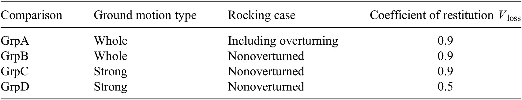
Note. This table compares different ground motion types, rocking cases, and coefficient of restitution.
Different ground motions have varying characteristics in terms of amplitude, frequency content, and duration. A sub-ser of relatively strong ground motion records was selected to group records with Peak Grond Accelerations (PGAs) larger than 0.3 g and a total duration of less than 60 seconds. The whole ground motion record set and the selected strong ground motion sub-set are plotted in Figure 6.
Duration versus peak ground acceleration (PGA) plot for whole ground motion records and selected strong motion records.

In the context of rocking behavior, the coefficient of restitution determines the amount of energy dissipated or transferred when the rocking block impacts or collides with the ground surface. A higher coefficient of restitution represents a more elastic collision, where a significant portion of the energy is restored after impact, therefore resulting in quicker oscillations and a longer duration for the system to reach a steady state of static equilibrium position. Conversely, a lower coefficient of restitution indicates a more inelastic collision, where a larger proportion of the energy is dissipated. A relatively high coefficient of restitution, 0.9, was assumed to model a more rapid and energetic response, leading to more visually distinguishable features in the predicted response-history plots. Additionally, a coefficient of restitution of 0.5 was selected to provide a comparison that aligns more closely with some real-world conditions.
Statistical analyses are performed for the four different cases (GrpA, GrpB, GrpC, and GrpD) outlined in Table 2, each with a different combination of ground motion type, rocking case, and coefficient of restitution. These analyses are carried out to quantitatively evaluate the performance of the PICNN framework in predicting rotations and angular velocities under different scenarios.
Equations (16) and (17) give the mathematical expression for mean absolute error and root-mean-square error:
 $$ \mathrm{MAE}=\frac{1}{N}\sum \mid {y}_i-\hat{y}\mid, $$
 $$ \mathrm{RMSE}=\sqrt{\mathrm{MSE}}=\sqrt{\frac{1}{N}\sum {\left({y}_i-\hat{y}\right)}^2}, $$
where $ {y}_i $
is the actual value and
$ {y}_i $
is the actual value and $ \hat{y} $
is the predicted value. MAE (Mean absolute error) calculates the difference between the original and estimated values by taking the mean absolute difference throughout the whole dataset under consideration. MSE (Mean Squared Error) represents the variance by squaring the average difference across the dataset. RMSE (Root Mean Squared Error) is the square root of MSE (Faber, Reference Faber2012). These metrics were calculated over the 50 points of the testing set.
$ \hat{y} $
is the predicted value. MAE (Mean absolute error) calculates the difference between the original and estimated values by taking the mean absolute difference throughout the whole dataset under consideration. MSE (Mean Squared Error) represents the variance by squaring the average difference across the dataset. RMSE (Root Mean Squared Error) is the square root of MSE (Faber, Reference Faber2012). These metrics were calculated over the 50 points of the testing set.
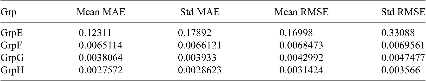
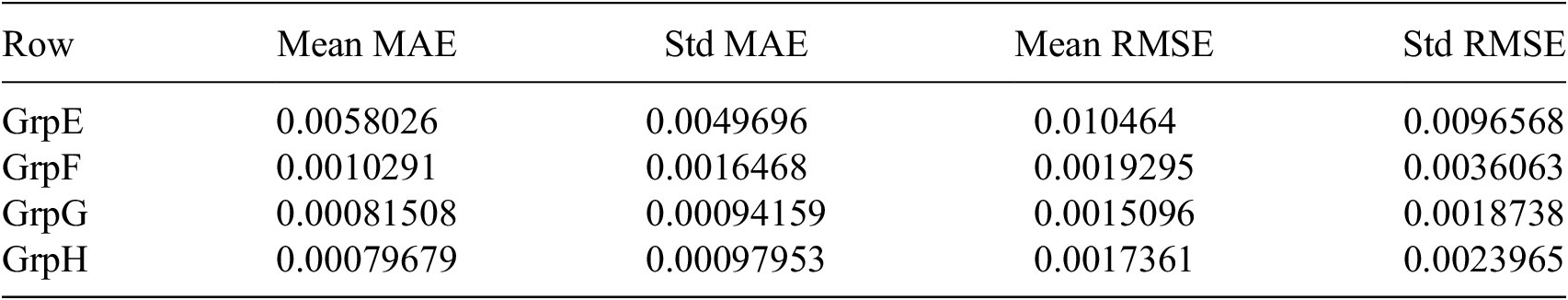
Tables 3 and 4 provide a comparison of the mean and standard deviation values for mean absolute error (MAE) and root mean squared error (RMSE) for different training groups related to $ \theta (t) $
and
$ \theta (t) $
and $ \dot{\theta}(t) $
. It can be seen that in both tables, a consistent improvement in the mean and standard deviation values for both MAE and RMSE is observed as one progresses from GrpA to GrpD. Among these comparison groups, GrpD (Strong ground motion, Nonoverturned rocking case,
$ \dot{\theta}(t) $
. It can be seen that in both tables, a consistent improvement in the mean and standard deviation values for both MAE and RMSE is observed as one progresses from GrpA to GrpD. Among these comparison groups, GrpD (Strong ground motion, Nonoverturned rocking case, $ {V}_{\mathrm{loss}}=0.5 $
) has the lowest mean MAE (
$ {V}_{\mathrm{loss}}=0.5 $
) has the lowest mean MAE ( $ \theta $
: 0.000289;
$ \theta $
: 0.000289; $ \dot{\theta} $
: 0.000722) and mean RMSE (
$ \dot{\theta} $
: 0.000722) and mean RMSE ( $ \theta $
: 0.000621;
$ \theta $
: 0.000621; $ \dot{\theta} $
: 0.00169) for both rotation and angular velocity, indicating higher accuracy in predicting angular displacement. Figures 7 and 8 show the box plot of MAE and RMSE for the rocking response prediction for all groups. Among them, GrpD shows the smallest box size and the lowest median for both angular displacement and angular velocity errors, this indicates that the prediction response from GrpD has the smallest spread and lower errors compared to the other groups, implying better predictive performance. GrpA generally exhibits the largest box sizes and highest medians, and have the widest range of outliers. The individual data points beyond the whiskers, which are plotted as red crosses in these figures, represent outliers in the dataset. These outliers indicate instances where the predicted values deviated significantly from the actual values, resulting in large prediction errors. In this context, the outliers specifically indicate the inability of the model to accurately predict overturned cases. The inability to accurately predict overturned cases is a significant finding as it highlights a limitation of the model in capturing and predicting such highly dynamic and unstable behavior.
$ \dot{\theta} $
: 0.00169) for both rotation and angular velocity, indicating higher accuracy in predicting angular displacement. Figures 7 and 8 show the box plot of MAE and RMSE for the rocking response prediction for all groups. Among them, GrpD shows the smallest box size and the lowest median for both angular displacement and angular velocity errors, this indicates that the prediction response from GrpD has the smallest spread and lower errors compared to the other groups, implying better predictive performance. GrpA generally exhibits the largest box sizes and highest medians, and have the widest range of outliers. The individual data points beyond the whiskers, which are plotted as red crosses in these figures, represent outliers in the dataset. These outliers indicate instances where the predicted values deviated significantly from the actual values, resulting in large prediction errors. In this context, the outliers specifically indicate the inability of the model to accurately predict overturned cases. The inability to accurately predict overturned cases is a significant finding as it highlights a limitation of the model in capturing and predicting such highly dynamic and unstable behavior.
Comparison of mean and standard deviation for MAE and RMSE ( $ \theta (t) $
)
$ \theta (t) $
)

Note. This table shows the mean and standard deviation values for MAE and RMSE for different training group data.
Comparison of mean and standard deviation for MAE and RMSE ( $ \dot{\theta}(t) $
)
$ \dot{\theta}(t) $
)

Note. This table shows the mean and standard deviation values for MAE and RMSE for different groups.
Box plot––root-mean-square error and mean absolute error in $ \theta (t) $
.
$ \theta (t) $
.

Box plot––root-mean-square error and mean absolute error in $ \dot{\theta}(t) $
.
$ \dot{\theta}(t) $
.

The correlation coefficient measures the strength of the association between two variables. Pearson’s correlation is a commonly used correlation coefficient in linear regression (Faber, Reference Faber2012). Another indicator commonly used to evaluate the performance of model for prediction is the Coefficient of determination (R 2), which is a measure of how well the variation in one variable can be explained by the variation in another variable. A value closer to 1 indicates that the model’s predictions are more accurate and closely match the actual data, with 1 indicating a perfect fit. The mathematical expression for both correlation coefficient and coefficient of determination (R 2) can be found below:
 $$ r=\frac{\sum \limits_{i=1}^n\left({x}_i-\overline{x}\right)\left({y}_i-\overline{y}\right)}{\sqrt{\sum \limits_{i=1}^n{\left({x}_i-\overline{x}\right)}^2\sum \limits_{i=1}^n{\left({y}_i-\overline{y}\right)}^2}}, $$
 $$ {R}^2=\frac{\mathrm{explained}\ \mathrm{variance}}{\mathrm{total}\ \mathrm{variance}}=\frac{\sum \limits_{i=1}^n{\left({\hat{y}}_i-\overline{y}\right)}^2}{\sum \limits_{i=1}^n{\left({y}_i-\overline{y}\right)}^2}, $$
where $ n $
is the number of data points,
$ n $
is the number of data points, $ {x}_i $
and
$ {x}_i $
and $ {y}_i $
are the data points for the two variables,
$ {y}_i $
are the data points for the two variables, $ \overline{x} $
and
$ \overline{x} $
and $ \overline{y} $
are the means of the two variables,
$ \overline{y} $
are the means of the two variables, $ {\hat{y}}_i $
is the predicted value of
$ {\hat{y}}_i $
is the predicted value of $ {y}_i $
, and
$ {y}_i $
, and $ \overline{y} $
is the mean of
$ \overline{y} $
is the mean of $ {y}_i $
.
$ {y}_i $
.
Figures 9–12 show the histogram graphs of correlation coefficient and coefficient of determination for the rocking response prediction ( $ \theta (t) $
and
$ \theta (t) $
and $ \dot{\theta}(t) $
) with Model 1. Generally speaking, these histograms show a concentration of correlation coefficients around higher values, indicating strong correlations between the predicted and actual values, which suggests that the framework predictions are accurate and align well with the observed data. The clustering of correlation coefficients around higher values (closer to 1) indicates that the PICNN Model 1 has a good fit and effectively predicts the overall rocking response. There is a consistent improvement in R and
$ \dot{\theta}(t) $
) with Model 1. Generally speaking, these histograms show a concentration of correlation coefficients around higher values, indicating strong correlations between the predicted and actual values, which suggests that the framework predictions are accurate and align well with the observed data. The clustering of correlation coefficients around higher values (closer to 1) indicates that the PICNN Model 1 has a good fit and effectively predicts the overall rocking response. There is a consistent improvement in R and $ {R}^2 $
histograms when moving toward GrpD, for both angular displacement and velocity, indicating that the framework is capable to capture the rocking response in non-overturning under more consistent ground motion with lower values of the coefficient of restitution. From the histogram plots, it is evident that the R
2 values for velocity predictions are generally higher and tend to cluster closer to 1 compared to the R
2 values for displacement predictions (dis). This suggests that the PICNN model is more accurate in predicting velocity responses than displacement responses.
$ {R}^2 $
histograms when moving toward GrpD, for both angular displacement and velocity, indicating that the framework is capable to capture the rocking response in non-overturning under more consistent ground motion with lower values of the coefficient of restitution. From the histogram plots, it is evident that the R
2 values for velocity predictions are generally higher and tend to cluster closer to 1 compared to the R
2 values for displacement predictions (dis). This suggests that the PICNN model is more accurate in predicting velocity responses than displacement responses.
Histogram graph for correlation coefficient ( $ \theta (t) $
).
$ \theta (t) $
).

Histogram graph for correlation coefficient ( $ \dot{\theta}(t) $
).
$ \dot{\theta}(t) $
).

Histogram graph for coefficient of determination ( $ \theta (t) $
).
$ \theta (t) $
).

Histogram graph for coefficient of determination ( $ \dot{\theta}(t) $
).
$ \dot{\theta}(t) $
).

Prediction performance metric in box plot.

Representative response-history plots for Group D.

Representative response-history plots for Group D. Cont.

Error distribution of prediction for training case GrpD.

Representative response-history plots for Group H.

Comparison of predicted and observed peak response parameters.

Guan et al. (Reference Guan, Burton, Shokrabadi and Yi2021) proposed a new novel performance metric, designed to examine the fraction of the dataset in which the relative difference between predicted and actual values falls below a predefined percentage, mathematically defined as follows:
 $$ {D}_{25\%}=\frac{countif\left[ abs\left(\frac{{\hat{y}}_i-{y}_i}{y_i}\right)\right]\leqslant 25\%}{N}, $$
where countif is a function that counts the number of the data points satisfying the condition in the square brackets, $ abs $
is the function that takes the absolute value of its argument,
$ abs $
is the function that takes the absolute value of its argument, $ {\hat{y}}_i $
is the predicted value,
$ {\hat{y}}_i $
is the predicted value, $ {y}_i $
is the actual value and N is the total number of data points. Table 5 summarizes the average percentage obtained from the Performance Metric, setting the threshold of 25% for the four case studies. It is found that GrpD (Strong ground motion, Nonoverturned rocking case,
$ {y}_i $
is the actual value and N is the total number of data points. Table 5 summarizes the average percentage obtained from the Performance Metric, setting the threshold of 25% for the four case studies. It is found that GrpD (Strong ground motion, Nonoverturned rocking case, $ {V}_{\mathrm{loss}}=0.5 $
) achieved the highest accuracy in predicting both rotation (
$ {V}_{\mathrm{loss}}=0.5 $
) achieved the highest accuracy in predicting both rotation ( $ \theta $
) and angular velocity (
$ \theta $
) and angular velocity ( $ \dot{\theta} $
), 92.683 and 92.836%, respectively. There is a consistent improvement in accuracy for both
$ \dot{\theta} $
), 92.683 and 92.836%, respectively. There is a consistent improvement in accuracy for both $ u $
and
$ u $
and $ {u}_t $
, indicating that stronger ground motions and lower values of
$ {u}_t $
, indicating that stronger ground motions and lower values of $ {V}_{\mathrm{loss}} $
lead to more accurate predictions.
$ {V}_{\mathrm{loss}} $
lead to more accurate predictions.
Relative difference presented in performance metric––25%

Note. This table compares different ground motion types and rocking cases.
The box plots shown in Figure 13 further support the observations regarding the accuracy of the predictions. The plot illustrates the distribution of the predefined performance metric for rotation ( $ \theta $
) and angular velocity (
$ \theta $
) and angular velocity ( $ \dot{\theta} $
) across the four groups. As seen in the box plot, GrpD exhibits the smallest spread of performances, indicating higher prediction accuracy for both
$ \dot{\theta} $
) across the four groups. As seen in the box plot, GrpD exhibits the smallest spread of performances, indicating higher prediction accuracy for both $ \theta $
and
$ \theta $
and $ \dot{\theta} $
compared to the other groups. Moreover, the median line of GrpD is the highest, indicating a better central tendency of the predicted values with respect to the actual data. Figures 14 and 15 show typical examples of response-history plots in Group D. It can be seen that Model 1 is capable of predicting the rocking response very well for a wide variety of ground-motion signatures.
$ \dot{\theta} $
compared to the other groups. Moreover, the median line of GrpD is the highest, indicating a better central tendency of the predicted values with respect to the actual data. Figures 14 and 15 show typical examples of response-history plots in Group D. It can be seen that Model 1 is capable of predicting the rocking response very well for a wide variety of ground-motion signatures.
In order to have a quantitative measure of the performance of the midfield PhyCNN framework and evaluate the success of the displacement and velocity measurement. The probability density function (PDF) of the normalized error distribution is calculated as follows:
 $$ p=\mathrm{PDF}\frac{y_{\mathrm{true}}-{y}_{\mathrm{predict}}}{\max \left(|{y}_{\mathrm{true}}|\right)}. $$
The same conclusion was reached when conducting the error distribution analysis, where angular velocity predictions exhibit higher accuracy compared to angular displacement predictions. It is found that the prediction error mainly located within the $ 0.5\% $
area for both displacement and velocity measurements. The corresponding confidence intervals (CI) are determined as
$ 0.5\% $
area for both displacement and velocity measurements. The corresponding confidence intervals (CI) are determined as $ 99.17 $
and
$ 99.17 $
and $ 100\% $
, respectively, as shown in Figure 16.
$ 100\% $
, respectively, as shown in Figure 16.
4.3. Model 2
Figure 17 shows the rocking response-history plots obtained with Model 2, which uses inputs of accelerations only. The red dotted line in these plots shows the reference output from the numerical simulation. It can be seen that the predicted angular acceleration has an excellent fit with the reference line, inditing good performance of Model 2. However, the predicted rotation directly shows relatively larger mismatches in amplitude although is still able to follow the general response pattern.
A statistical analysis was also performed on the predictions of Model 2 to get a quantitative understanding of its performance. The same optimization study implementing four training groups defined before was followed, as shown in Tables 6–8. $ \mathrm{The}\;{D}_{25\%} $
performance metric between the predicted rocking response and the reference true value was calculated with the selected threshold of 25%, as before. Generally speaking, even for the worst cases, the percentage accuracy for prediction of the rocking angular acceleration is still above 80% in most cases (Table 6) and the error values (Tables 7 and 8) are acceptable.
$ \mathrm{The}\;{D}_{25\%} $
performance metric between the predicted rocking response and the reference true value was calculated with the selected threshold of 25%, as before. Generally speaking, even for the worst cases, the percentage accuracy for prediction of the rocking angular acceleration is still above 80% in most cases (Table 6) and the error values (Tables 7 and 8) are acceptable.
Relative difference performance metric $ {D}_{25\%} $

Note. This table compares different ground motion types and rocking cases.
Comparison of mean and standard deviation for MAE and RMSE ( $ \theta (t) $
)
$ \theta (t) $
)
Note. This table shows the mean and standard deviation values for MAE and RMSE for different training group data.
Comparison of mean and standard deviation for MAE and RMSE( $ \ddot{\theta}(t) $
)
$ \ddot{\theta}(t) $
)
Note. This table shows the mean and standard deviation values for MAE and RMSE for different groups.
5. Discussion
We have proposed two PICNNs models in the previous sections, and have performed statistical, comparative and optimization analyses on them. The results of these analyses provided valuable insights, but it is important to note that limitations were also observed. It has been shown, for example, that the accuracy of the predictive framework proposed can be significantly influenced by the duration of the ground motion, the possibility of overturning, and the value of the coefficient of restitution.
The characteristics of the input ground motion (duration, amplitude and frequency) have shown a significant influence on the performance of the PICNNs. The amplitude and frequency of ground motion affects the total amount of input data available for analysis, and a stronger ground motion can facilitate a better learning of the seismic rocking response. On the other hand, a weaker ground motion may not capture the full range of dynamic behavior needed for the neural network to establish a good prediction. In this study, a relative stronger ground motion record dataset (PGA larger than 0.3 g) was selected for training and available to predict the rocking seismic response under the ground motion. As shown in Table 5, using a stronger ground motion input, the relative differences performance metric $ {D}_{25\%} $
of both rotations
$ {D}_{25\%} $
of both rotations $ \theta $
an angular velocity
$ \theta $
an angular velocity $ \dot{\theta} $
increased by 3 and 8%, respectively. The duration of ground motion affects the temporal context available for the model to learn from, potentially influencing the model’s ability to capture long-term dynamic effects and transient responses without overwhelming the training process. A broader range of duration for ground motion input can introduce more complexity and variability in training the model, which results in larger uncertainties. Striking the right balance in selecting ground motions with a suitable range of characteristics is essential for the current PICNNs framework to generalize well and make more robust and accurate predictions.
$ \dot{\theta} $
increased by 3 and 8%, respectively. The duration of ground motion affects the temporal context available for the model to learn from, potentially influencing the model’s ability to capture long-term dynamic effects and transient responses without overwhelming the training process. A broader range of duration for ground motion input can introduce more complexity and variability in training the model, which results in larger uncertainties. Striking the right balance in selecting ground motions with a suitable range of characteristics is essential for the current PICNNs framework to generalize well and make more robust and accurate predictions.
The statistical analysis conducted in the previous section also showed that the behavior of rocking (overturned or non-overturned) would determine the performance of our deep PICNNs. The physics restraints embedded in the framework spring from the governing equation of motion, however, as it does not explicitly incorporate information about overturned or non-overturned cases, the PICNNs would not be able to identify or differentiate between these cases. The ability of the PICNN framework to capture and identify rocking behavior would primarily depend on the availability and representation of relevant data in the training set. If the training data include large examples of overturned or non-overturned cases, the network could learn to associate certain input patterns with rocking behavior. However, this understanding would be implicitly learned from the data rather than explicitly encoded through the physics-informed component of the deep neural network. Alternatively, a parallel regression model could be used to distinguish between overturning and non-overturning cases in the first instance, leaving the proposed PICNN to concentrate on learning the main features of the non-overturning responses.
The value of coefficient restitution selected in constructing the database for training also plays a substantial role when analyzing the performance of PICNNs framework in predicting rocking seismic response. The coefficient of restitution quantifies the energy dissipation and restitution characteristics during impacts, and directly affects the dynamic response of the rocking block. A higher coefficient of restitution tends to lead to more pronounced rocking motion with greater peak displacements and accelerations. On the other hand, a lower coefficient of restitution results in reduced rocking motion and dampened response. A value of 0.5 is commonly employed in experiments to represent approximately 50% of the kinetic energy is preserved or restored during the interaction between the rocking block and the ground surface. In the numerical validation section, it was observed that the accuracy of the PICNN framework for predicting rocking response in terms of angular displacement, velocity, and acceleration improved when a lower coefficient of restitution of 0.5 was selected, closer to what is typically encountered in real-world applications.
As observed in some of the angular displacement response-history plots presented above, the chattering effect occurs in the numerical simulation can impact the accuracy and reliability of the PICNNs. Chattering refers to the occurrence of rapid and irregular oscillations during low-amplitude oscillations or transitions in the system (Giouvanidis et al., Reference Giouvanidis, Dimitrakopoulos and Lourenço2022). Capturing chattering in the rocking response has proven to be particularly challenging with the neural networks explored as the discontinuities and abrupt changes that occur during the transient behavior of rocking structures can be very hard to model. The chattering phenomenon in PICNNs predictions for rocking behavior can cause unstable and unreliable results, hindering the interpretation and utilization of the outputs. It can also cause convergence difficulties during training, impeding the network optimization process. Additionally, the sensitivity of chattering to small changes in initial conditions can pose challenges, as slight variations can lead to divergent predictions and significant impacts on the prediction of rocking behavior. To address the issue of chattering when implementing PICNNs to predict the seismic rocking response, possible strategies include improving data representation by incorporating chattering-related dynamics, refining the loss functions to account for chattering, and adjusting network architecture and regularization techniques (dropout, weight decay, or adaptive learning rate algorithms) to enhance stability. Additionally, conducting sensitivity analyses on initial conditions and input parameters helps understand the system’s sensitivity to chattering and aids the interpretation of the predictions (Pizarroso et al., Reference Pizarroso, Portela and Muñoz2022). Also, several learning rates, batch sizes, and number of layers were tested, the PICNNs implemented here can be further tuned by evaluating their performance on a wider set of ground-motion and rocking response data.
Another interesting possibility is related to the model’s ability to predict global statistics of rocking responses even if individual response-history signatures deviate from the observations. This is explored in Figure 18 that shows a comparison of peak rotation and peak acceleration values extracted from the predicted response series and their numerical observations. In both cases, duration is used as a ground motion IM following our previous observation regarding its role in shaping the PICNN’s predictions of rocking responses. It is clear from this figure, that good levels of estimation are achieved by both models. These encouraging results open the door for the use of PICNN models for the estimation of probabilities of exceedance of certain peak response levels (i.e., failure) even if overturning probabilities are not well captured.
6. Conclusion
This article has demonstrated that PICNNs are capable of simulating the hard-nonlinear problem of rigid blocks engaged in seismically induced rocking motion. The work and results presented have shown, for the first time, that using the deep learning method of CNN (convolutional NN) with physics constraints encoded offers a simplified and efficient alternative for predicting the rocking response over a range of real ground-motion records. The article presents a way to integrate the underlying physics of rocking dynamics into the CNN architecture to guide model training. The proposed deep PICNN model consists of five convolution layers and three fully connected layers for data interpretation, a graph-based tensor differentiator was used for deriving the angular acceleration with encoded physics constraints. Two models have been proposed. Model 1 assumes that the entire set of response histories including rotations and rotational velocities are available for training, while Model 2 assumes that only acceleration measurements are available.
Overall, the rocking response predicted by the proposed PICNN is in good agreement with the numerical model when training with only one rocking feature for nonoverturning cases under consistent strong ground motions. The robustness of the proposed technique is illustrated by training the PICNN with mixed/limited datasets, stressing the importance that the quantity and quality of data has on the prediction performance.
On the other hand, it was found that the current developed deep PICNN cannot accurately predict the rocking response of blocks that overturn since it fails to capture the ever-increasing amplitude in drifts and rotations. However, it is expected that in those cases, an alternative regression model could be used to distinguish first, in a prior step, between overturning and non-overturning cases, and the currently proposed PICNN can then be used to estimate the response history of non-overturning blocks.
The results of the error distribution analysis performed indicate that the deep PICNN framework performs better when estimating the angular acceleration than the block rotation with a confidence interval of $ 100 $
and
$ 100 $
and $ 99.17\% $
, respectively. Furthermore, it was found that the proposed deep PICNN framework can significantly reduce computational costs. The model is more generalizable and has lower training expenses than traditional numerical FEA modeling. It is important to note that in this study, the proposed PICNN model has been verified by means of widely accepted numerical procedures, and further investigations should be performed in order to confirm experimental results which would strengthen the confidence on the application of PICNN to predict hard nonlinear problems like rocking and to estimate future states of motion, especially with Model 2 which is closer to real applications.
$ 99.17\% $
, respectively. Furthermore, it was found that the proposed deep PICNN framework can significantly reduce computational costs. The model is more generalizable and has lower training expenses than traditional numerical FEA modeling. It is important to note that in this study, the proposed PICNN model has been verified by means of widely accepted numerical procedures, and further investigations should be performed in order to confirm experimental results which would strengthen the confidence on the application of PICNN to predict hard nonlinear problems like rocking and to estimate future states of motion, especially with Model 2 which is closer to real applications.
Author contribution
Conceptualization: All authors; Data curation: S.S.; Investigation: S.S.; Methodology: C.M.; Project management: C.M.; Supervision: C.M.; Writing—original draft: All authors; Writing—review and editing: All authors. All authors approved the final submitted draft.
Competing interest
The authors declare no competing interests exist.
Data availability statement
The data that support the findings of this study are available from the authors upon request.
Funding statement
This work received no specific grant from any funding agency, commercial or not-for-profit sectors.
Ethical standard
The research meets all ethical guidelines, including adherence to the legal requirements of the study country.


 Open access
Comments
No Comments have been published for this article.