Ice-core and borehole site input data

Temporally sequential measurements of borehole inclination, from which the vertical profile of the horizontal velocity is obtained, are a valuable adjunct to the ice-core and borehole data streams routinely obtained during deep drilling of ice cores for palaeoclimate records. The combined datasets are ideally suited to evaluating the dynamics of ice masses. Here we use data from the DSS ice core, drilled 4.7 km south-southwest of the Law Dome summit in East Antarctica (Fig. 1), to evaluate the AGA, TNNI, CAFFE and B2013 flow relations. For each relation we calculate depth profiles of the shear stress, aligned parallel to the surface flow direction, and the vertical compression deviatoric stress. Input data include strain rates derived from the borehole inclination; ice-core c-axis orientation fabrics; borehole temperatures; and surface measurements of the drill-site ice flow direction, velocity and strain rate (Fig. 2; Table 1). To assist assessment of the DSS-site stress estimates we use strain-rate and fabric data from laboratory ice deformation experiments (Reference Budd, Warner, Jacka, Li and TreverrowBudd and others, 2013) to calculate the corresponding applied stresses; unlike the stresses in an ice sheet, the applied stresses in laboratory experiments are known.

Table 1. DSS borehole site and ice-core information (Reference Morgan, Wookey, Li, Van Ommen, Skinner and FitzpatrickMorgan and others, 1997, Reference Morgan, Van Ommen, Elcheikh and Li1998)

Fig. 1. Location of the Dome Summit South (DSS) ice-core site (yellow star) at an elevation of 1370 m on Law Dome, East Antarctica (see inset). The red box indicates a 25 km × 25 km region surrounding the Law Dome summit. Within this region the blue line is a portion of the flowline which extends from the dome summit through the DSS ice-coring site and downstream towards Vanderford Glacier. The background image is from the Landsat Image Mosaic of Antarctica (Reference BindschadlerBindschadler and others, 2008); 100 m elevation contours are from Reference Bamber, Gomez-Dans and GriggsBamber and others (2009).

Fig. 2. DSS ice-core and borehole data as a function of ice equivalent depth. Bedrock is estimated to occur at an ice equivalent depth of 1198.5 ± 20 m. (a) Borehole temperature (Reference Morgan, Van Ommen, Elcheikh and LiMorgan and others, 1998). (b) Shear strain rate, derived from borehole inclination measurements projected onto the direction parallel to the drill-site surface flow direction (Reference Morgan, Van Ommen, Elcheikh and LiMorgan and others, 1998). The smoothed shear strain-rate profile (bold black line) is a five-point running mean. The vertical strain rate is derived from the horizontal velocity profile and surface accumulation rate using Eqn (3). (c) Orientation tensor eigenvalues, a_i , were determined from the c-axis vector distributions measured for each of 185 thin sections obtained from the DSS ice core (Reference LiLi, 1995; Reference Morgan, Wookey, Li, Van Ommen, Skinner and FitzpatrickMorgan and others, 1997). The triplets of points at each depth are the eigenvalues, a_i , of the second-order orientation tensor, where a ₁ > a ₂ > a ₃. The bold lines represent eigenvalues determined from fivemember composite fabrics, typically containing N ≈ 500 individual c-axes.

In the following we present ice-core and borehole data as a function of ice equivalent depth,

(2)

where ρ(χ) is the firn/ice density at actual depth χ, ρ _ice = 917 kg m⁻³ is the ice density and is the total ice-sheet thickness. Below the firn–ice transition at ∼40 m the ice equivalent depth has a constant offset of −21.5 m relative to the actual depth (Reference Van Ommen, Morgan and CurranVan Ommen and others, 2004; Reference RobertsRoberts and others, 2015).

Borehole and surface measurements

Figure 2a shows how ice temperature at DSS increases from a mean annual surface value of −21.8 C to −6.9 C at the bottom of the borehole. The DSS core was drilled to near bedrock, and small fragments of rock were recovered from the lowest core section. Comparison of the borehole depth (1195.6 m) and estimates of the total ice thickness based on radio-echo sounding (RES; 1220 ± 20 m (Reference Morgan, Wookey, Li, Van Ommen, Skinner and FitzpatrickMorgan and others, 1997)) suggest bedrock was <45 m below the bottom of the borehole. From this it may reasonably be assumed that the basal ice temperature is less than the in situ pressure-melting point, despite the relatively high geothermal flux of 72 mW m⁻² at the DSS site (Reference Van Ommen, Morgan, Jacka, Woon and ElcheikhVan Ommen and others, 1999).

Figure 2b (grey line) shows the shear strain-rate profile derived from the borehole inclination projected onto a plane parallel to the ice surface velocity vector of 2.04 ± 0.11 m a⁻¹ at 225 ± 3°, determined from 4 months of GPS measurements during the 1995/96 austral summer (Reference Morgan, Van Ommen, Elcheikh and LiMorgan and others, 1998). The small-scale fluctuations and negative values of the shear strain rate at depths above 300 m are a consequence of noise in the inclination data where deformation rates are low (Reference Morgan, Van Ommen, Elcheikh and LiMorgan and others, 1998). The borehole movement and hence shear strain rate in the direction transverse to the surface flow (not shown) has a similar magnitude to the total measurement error and is considered negligible (Morgan and others,1998). The surface strain-rate components are (3.22 ± 0.016) × 10⁻⁴ a⁻¹ in the line of flow and (4.50 ± 0.027) × 10⁻⁴ a⁻¹ transverse to the surface flow direction (Reference Morgan, Van Ommen, Elcheikh and LiMorgan and others, 1998). We specify a coordinate system at the DSS site where z is the vertical (upward) direction with x and y, respectively, parallel and transverse to the surface flow direction.

The shear strain rate does not increase monotonically to the bed; a broad maximum occurs at ∼1000 m depth, or ∼180 m above bedrock (Fig. 2b). The transition to lower shear strain rates below ∼1000 m is not accompanied by any corresponding large-scale changes in ice chemistry or soluble-impurity content, rather it is associated with stress relaxation towards the bed due to flow over undulating bedrock topography at Law Dome (e.g. Reference Budd and JackaBudd and Jacka, 1989; Reference Morgan, Wookey, Li, Van Ommen, Skinner and FitzpatrickMorgan and others, 1997). Similar maxima in the shear strain rate ∼130 m above the bed have been observed in the BHF, BHC-1 and BHC-2 boreholes drilled at near-coastal sites along a flowline from Law Dome summit towards Cape Folger (Reference Russell-Head and BuddRussell-Head and Budd, 1979; Reference EtheridgeEtheridge, 1989), where the ice thickness is ∼300–385 m. Modelling indicates that these peak shear strain rates are associated with a corresponding maximum in the shear stress and that the onset of a transition to lower shear strain rates (and stresses) with depth is related to the magnitude of the bedrock undulations.

Superimposed on the decreasing shear strain rate at depths below 1000 m is a narrow band between 1110 and 1124 m where the shear rate is about five times greater than that in ice immediately above and below (Fig. 2b). The ice-core δ¹⁸O record indicates this ice was deposited during the Last Glacial Maximum (LGM) and compared with the overlying Holocene ice has (1) significantly smaller mean grain area, (2) a strong vertical single-maximum crystal orientation fabric and (3) particle concentrations two orders of magnitude higher (Reference Morgan, Van Ommen, Elcheikh and LiMorgan and others, 1998). Reference Li, Jacka and MorganLi and others (1998) have shown that the higher insoluble impurity concentrations associated with this layer are sufficient to retard rates of microstructural evolution. Unlike the ice immediately above and below, this allows the vertical single-maximum pattern of c-axis orientations, which originated upstream of the DSS site, to persist within this narrow band of ice. This high level of polycrystalline anisotropy, combined with higher temperatures closer to the bed, results in a discrete band from 1100 to 1124 m with the highest shear strain rates within the DSS borehole (Fig. 2b).

Vertical strain rates

The vertical strain-rate profile, (Fig. 2b), was not determined by direct measurement and is obtained from Eqn (3) assuming steady-state conditions and ice incompressibility (e.g. Reference ReehReeh, 1988):

(3)

where is the annual accumulation rate, is the mean of the horizontal velocity depth profile, u(z), z _T is the ice thickness, and the horizontal velocity shape function ψ(z) relates u(z) to as described below. Assuming that ψ(z) only varies gradually along the line of flow,

(4)

and the last term in Eqn (3) can be neglected. As the surface slope at the DSS site is low (α ∼ 0.0051), the second term in Eqn (3) is also negligible since is about two orders of magnitude greater than (Table 1). The assumption that Law Dome is in steady state and has a stable geometry is reasonable since the DSS ice-core isotope and chemistry records indicate a stable annual accumulation rate over the past ∼6.8 ka (Reference Van Ommen, Morgan and CurranVan Ommen and others, 2004). It follows that the vertical strain rate can be estimated from the first term in Eqn (3).

The near-surface (75.6 m actual depth) vertical strain rate of , which was derived from the bore-hole inclination data, agrees favourably with the independently determined surface GPS value of (Table 1; Reference Morgan, Van Ommen, Elcheikh and LiMorgan and others, 1998).

Ice-core measurements

The DSS ice-core fabric data used in this study include c-axis orientations from 185 thin sections obtained at ∼6m intervals between 117 m depth and the bottom of the ice core (Fig. 2c; Reference LiLi, 1995; Reference Morgan, Van Ommen, Elcheikh and LiMorgan and others, 1998). All fabrics were measured manually at the time of drilling using a Rigsby stage, with each fabric typically restricted to N ≈ 100 individual c-axis orientations due to the laborious nature of the measurement procedure (Reference Morgan, Wookey, Li, Van Ommen, Skinner and FitzpatrickMorgan and others, 1997). For certain sections, mainly at depths below ∼1040 m, the number of grains within an individual fabric was <100 due to the combined effects of higher temperatures and stress relaxation on grain growth, leading to higher mean grain sizes and a reduction in the total number of grains within a single thin section.

Following Reference WoodcockWoodcock (1977), the eigenvalues a_i (i = 1, 2, 3) of the normalized second-order c-axis orientation tensor,

(5)

are used to illustrate fabric evolution with depth at DSS (Fig. 2c).

The eigenvalues of Λ are related as a ₁ + a ₂ + a ₃ = 1, where by convention 0 ≤ a ₃ ≤ a ₂ ≤ a ₁ ≤ 1. Because the eigenvalues describe the degree of clustering of c-axis orientations about their respective eigenvectors they are related to the fabric shape. The eigenvector, , of the maximum eigenvalue, a ₁, is the direction about which the distribution of orientations is minimized, whilst is the direction about which the distribution is largest. As a ₁ → 1, the distribution of orientations becomes smaller, i.e. fabrics become stronger or more concentrated. It follows for an isotropic (random) distribution of orientations that . The area of individual grains was not determined during orientation measurements (Reference LiLi, 1995), so volume weighting of the orientation data (e.g. Reference Durand, Gagliardini, Thorsteinsson, Svensson, Kipfstuhl and Dahl-JensenDurand and others, 2006) was not possible and all orientations contribute equally to (Fig. 2c).

Several general comments can be made regarding the DSS ice core c-axis distribution:

1. 1. Near-surface fabrics are not isotropic because a ₁ ≫ a ₂ ≈ a ₃. Non-random patterns of orientations near the firn-to-ice transition are most likely influenced by a range of factors related to accumulation, grain growth and deformation processes.

2. 2. All fabrics down to ∼1000 m are vertically clustered, with approximately parallel to the long axis of the core. The strength of the single-maximum fabrics increases with depth from 550 m to 1000 m. These fabrics are consistent with the increasingly high shear strain rates over the same depth range. Small-scale fluctuations in fabric strength (Fig. 2c) are closely coupled to changes in the grain size, with smaller grain sizes associated with stronger fabrics (Reference Morgan, Wookey, Li, Van Ommen, Skinner and FitzpatrickMorgan and others, 1997).

3. 3. Down to ∼1000 m, fabrics are approximately transversely isotropic. Based on the surface flow divergence, indicated by (Table 1), the consistent difference of ∼0.04 between a ₂ and a ₃ may be related to some transverse spreading of the fabrics; however, the azimuthal orientation of thin sections is not available to confirm this.

4. 4. Below ∼1040 m multiple-maxima fabrics are observed. These are consistent with topographically induced stress relaxation and increasing ice temperatures at depth resulting in recrystallization, including significant grain growth (Reference LiLi, 1995; Reference Morgan, Wookey, Li, Van Ommen, Skinner and FitzpatrickMorgan and others, 1997). Multiple-maxima fabrics are not well described by the orientation tensor eigenvalues; however, a reduction in a ₁ and an increase in the difference between a ₂ and a ₃ below ∼1040 m are indicative of a transition from the single-maximum fabrics associated with the overlying high shear zone.

Background to the flow relations

The AGA, TNNI and CAFFE flow relations have been selected for comparison with the B2013 flow relation because each differs in the degree to which physically based interpretations of grain-scale deformation and recovery processes are incorporated into the formulation. These flow relations may be broadly classified as homogenization schemes since the strain-rate response of a polycrystalline aggregate is based on consideration of the orientation relationship between individual grains (represented by crystallographic c-axis vectors) and the macroscopic deviatoric stress tensor. Both the AGA and TNNI relations define the stress acting on an individual grain in terms of its c-axis orientation relative to the applied stress in conjunction with a consideration of neighbour grain orientation effects. The CAFFE flow relation is a generalization of the Reference GlenGlen (1958) flow relation using grain orientations in conjunction with the deviatoric stress tensor to specify a scalar anisotropic enhancement factor. The B2013 relation is an empirical parameterization based on deformation experiments conducted in a range of stress configurations using laboratory-made ice.

Several other anisotropic flow relations could have been considered for inclusion in this study (e.g. Reference LileLile, 1984; Reference Van der Veen and WhillansVan der Veen and Whillans, 1994; Reference Svendsen and HutterSvendsen and Hutter, 1996; Reference Gagliardini and MeyssonnierGagliardini and Meyssonnier, 2000; Reference GödertGödert, 2003; Reference StaroszczykStaroszczyk, 2003; Reference Gillet-Chaulet, Gagliardini, Meyssonnier, Montagnat and CastelnauGillet-Chaulet and others, 2005; Reference PettitPettit and others, 2011; Reference Martín, Gudmundsson and KingMartín and others, 2014). In many anisotropic flow relations, fabrics are represented by a c-axis orientation distribution function (ODF). For some flow relations (such as CAFFE) it is possible to also work directly with discrete c-axis vectors instead of an ODF. For other flow relations it is not straightforward to make the translation to a vector description of the c-axis distribution. For reasons of simplicity, a constrained form of ODF, where the anisotropy is described by a limited number of variables, is often specified. This can introduce symmetry limitations on the ODF (e.g. a restriction to only transversely isotropic orientation patterns), with the result that naturally occurring fabrics that do not satisfy these criteria are not adequately described. Since a specific aim of this study is to compare the empirical B2013 relation to microscale flow relations using the DSS ice-core crystal orientation fabric data, we have restricted our analysis to a subset of candidate flow relations where the deforming polycrystalline aggregate can be described by a discrete distribution of c-axis orientation vectors.

AGA flow relation

In the AGA flow relation individual grains are assumed to deform only by glide on crystallographic basal planes, normal to the c-axis. The outer product of the basal glide direction, m , and the crystallographic c-axis vectors, c , define a geometrical factor tensor G _(g) for a grain,

(6)

G _(g) is the origin of anisotropy in the AGA relation and describes the geometric connection between the applied stress tensor on a grain, σ _(g), and the scalar magnitude of the resolved shear stress, τ _(g), on the basal plane of a grain:

(7)

where X : Y denotes the generalized inner product X _ij Y _ji . Because grains are assumed to deform by basal glide alone, the temperature-dependent flow parameter, β_S , for easy glide of single crystals is used in the definition of the strainrate tensor for a grain (Reference Azuma and Goto-AzumaAzuma and Goto-Azuma, 1996):

(8)

where is the symmetrization of G and

(9)

Here is a material-dependent parameter, specific to single-crystal deformation, which is several orders of magnitude higher than corresponding values for polycrystalline ice deformation (e.g. Reference Cuffey and PatersonCuffey and Paterson, 2010, ch. 3.4). is largely determined by the concentration of soluble and insoluble impurities (e.g. Reference Jones and GlenJones and Glen, 1969; Reference Trickett, Baker and PradhanTrickett and others, 2000b), Q _s is a single-crystal creep activation energy and R is the universal gas constant. Equation (8) includes the single-crystal creep power-law stress exponent, n, and from the derivation of Reference Azuma and Goto-AzumaAzuma and Goto-Azuma (1996) this value should apply in Eqn (8) and later in Eqn (11). Based on Reference WeertmanWeertman (1983), Reference Azuma and Goto-AzumaAzuma and Goto-Azuma (1996) assume n = 3 for single crystal deformation. Analyses of single-crystal deformation by Reference Duval, Ashby and AndermanDuval and others (1983) and Reference TreverrowTreverrow (2009) demonstrate that a stress exponent of n = 2 is appropriate for easy glide of single crystals, suggesting that this value should have featured in the AGA relation. For consistency with the flow relation presented by Reference Azuma and Goto-AzumaAzuma and Goto-Azuma (1996), and the other relations considered in this study, we use the more widely accepted value of n = 3 for polycrystalline deformation.

Reference Azuma and Goto-AzumaAzuma and Goto-Azuma (1996) proposed an empirical relationship for σ _(g) as a function of the macroscopic stress tensor, σ , and the c-axis orientation of the grain and its nearest neighbours, based on experimental observations of polycrystalline ice deformation (Reference AzumaAzuma, 1995). This relationship, along with the assumptions

(10)

where N _T is the number of grains in a polycrystalline aggregate, defines the macroscopic strain rate,

(11)

Thus the macroscopic anisotropy of the AGA relation is determined by the arithmetic mean of G _(g) for each grain. The assumptions leading to Eqn (10) are significant since they enable expressions for the redistribution of the applied stress on each grain, based on neighbour grain c-axis orientations, to be eliminated from the calculation of . This greatly simplifies numerical implementation of the AGA flow relation as c-axis data only enter into the calculation of G .

TNNI flow relation

Similar to the AGA flow relation, in the TNNI flow relation individual grains are assumed to deform only by glide on basal planes and the polycrystalline strain rate is determined from the homogenization of individual grain deformations. Of the flow relations considered in this study, the TNNI relation incorporates the most physically motivated description of grain-scale deformation processes. The deformation of individual grains is based on the slip rate for each crystallographic basal slip system and includes a parameterization of c-axis dependent nearest-neighbour grain interactions.

The anisotropy of the TNNI flow relation is derived from the Schmid tensor, R ^s , for each basal slip system within a grain,

(12)

where c is the crystallographic c-axis vector, b ^s is the Burgers vector, parallel to the crystallographic slip direction, and the index s = 1, 2, 3 denotes quantities associated with each a-axis slip system within a grain. The Schmid tensor links the macroscopic stress, σ , to the shear stress, , resolved onto the basal plane of each grain,

(13)

The quantity, , is analogous to τ _(g) in the AGA flow relation, Eqn (7). Reference ThorsteinssonThorsteinsson (2002) defined a parameterization of grain interaction that influences the magnitude of anisotropic flow enhancement in the TNNI flow relation. The softness parameter for a grain,

(14)

is a function of the resolved shear stresses on a reference grain, , and each of its six nearest neighbours, . The grain interaction parameters for the reference grain, C ₀, and each of its nearest neighbours, C _n, define the extent to which neighbour grain interactions influence the redistribution of applied stresses onto each grain. Reference ThorsteinssonThorsteinsson (2002) specifies three levels of nearest-neighbour grain interaction (NNI):

1. 1. No NNI. C ₀ = 1 and C _n = 0. No neighbour grain interaction, , corresponding to a homogeneous stress condition.

2. 2. Intermediate NNI. C ₀ = 6 and C _n = 1. The relative contribution of the reference grain to is equivalent to that of all the neighbour grains combined.

3. 3. Full NNI. C ₀ = 1 and C _n = 1. The relative contribution of all grains to is equivalent.

Full NNI produces the highest levels of anisotropic flow enhancement and is used in the following analyses.

The velocity gradient tensor, L _(g), of a single crystal is the sum of the velocity gradient tensor for each slip system,

(15)

where the temperature dependent term,

(16)

is that specified in the Reference GlenGlen (1958) flow relation, Eqn (1). Q is an activation energy for the creep of polycrystalline ice and R and T are as previously defined. The pre-exponential term A ₀ can be determined empirically from the secondary creep of isotropic polycrystalline ice and is assumed to be dependent upon material-specific factors including ice density and the size and concentration of soluble and insoluble impurities (e.g. Reference Budd and JackaBudd and Jacka, 1989; Reference Cuffey and PatersonCuffey and Paterson, 2010). The constant B (Eqn (15)) is an arbitrary tuning parameter that ensures the flow relation reproduces physically-accurate strain rates (Reference ThorsteinssonThorsteinsson, 2001). The macroscopic velocity gradient, L, for a polycrystalline aggregate of N _T grains is the arithmetic mean of the individual grain velocity gradients (Reference ThorsteinssonThorsteinsson, 2002):

(17)

and the polycrystalline strain rate is

(18)

CAFFE flow relation

In the CAFFE flow relation, individual grains are also assumed to deform by basal glide; however, unlike the AGA and TNNI flow relations the polycrystalline strain rate is not derived from a homogenization of individual grain deformations. The magnitude of the applied deviatoric stress S resolved on the basal plane of a grain is used to define a deformability index, D( c ), for each grain, which quantifies the proportion of the applied stress able to drive deformation of a grain specified by its c-axis vector, c.

(19)

where S_t is the magnitude of the resolved basal deviatoric stress component. An array of c-axis vectors can be described by an orientation distribution function (ODF) that quantifies the volume fraction of c-axis orientations. By integrating the single crystal deformability, D( c ), weighted by the ODF over the unit sphere, , the polycrystalline deformability D is obtained (Reference Seddik, Greve, Placidi, Hamann and GagliardiniSeddik and others, 2008; Reference Placidi, Greve, Seddik and FariaPlacidi and others, 2010). By expressing integrals as summations over the N _T individual crystals in a polycrystalline aggregate, the macroscopic deformability, D, can also be determined directly,

(20)

The macroscopic deformability is used to determine a nonlinear, scalar enhancement function, E(D), for the Reference GlenGlen (1958) flow relation in Eqn (1). E(D) is defined over the interval ,

(21)

where E _min and E _max are user-defined limits of enhancement, such that E(D) has the following fixed points:

1. 1. D = 0, E(0) = E _min. The minimum enhancement value is returned when there is no resolved shear stress on the basal planes of grains. To avoid numerical issues Reference Placidi, Greve, Seddik and FariaPlacidi and others (2010) recommend selecting 0 < E _min < 0.1.

2. 2. D = 1, E(1) = 1. The factor of in Eqn (19) ensures that D = 1 for an isotropic c-axis distribution, resulting in an enhancement of E = 1. In this situation the CAFFE flow relation, Eqn (22), reduces to the Reference GlenGlen (1958) flow relation.

3. 3. . The maximum deformability returns the theoretical maximum enhancement, E_max, when the applied stress is entirely resolved onto the basal planes of all grains. This corresponds to an idealized scenario where all grains in a polycrystalline aggregate have identical c-axis orientations that are normal to an applied simple shear stress.

Reference Placidi, Greve, Seddik and FariaPlacidi and others (2010) suggest E _max ≈ 10, based on experiments by Reference Pimienta, Duval and LipenkovPimienta and others (1987) on samples from the Vostok (East Antarctica) ice core with a strong single-maximum crystal orientation fabric. Other field and laboratory observations of simple shear strain-rate enhancement suggest potential E _max values ranging from ∼4 to 12 (e.g. Reference Russell-Head and BuddRussell-Head and Budd, 1979; Reference DuvalDuval, 1981; Reference Azuma and HigashiAzuma and Higashi, 1984; Reference LileLile, 1984; Reference Dahl-Jensen and GundestrupDahl-Jensen and Gundestrup, 1987; Reference Pimienta, Duval and LipenkovPimienta and others, 1987; Reference Li, Jacka and BuddLi and others, 1996; Reference Morgan, Van Ommen, Elcheikh and LiMorgan and others, 1998; Reference Thorsteinsson, Waddington, Taylor, Alley and BlankenshipThorsteinsson and others, 1999). Here we specify a mid-range value of E _max = 8 based on the compilation of Reference Treverrow, Budd, Jacka and WarnerTreverrow and others (2012). This value is consistent with selection of E _s = 8, for the conceptually similar E _s parameter in the B2013 flow relation.

Reference FariaFaria (2008) has demonstrated how the polycrystalline deformability, D (Eqn (20)), provides the anisotropic foundation of the scalar enhancement factor, E(D). The polycrystalline strain rate is

(22)

where the temperature-dependent flow parameter A(T) is as defined previously and the stress exponent n = 3. Due to the collinear relationship between components of and S, the CAFFE flow relation, Eqn (22), can readily be inverted to express S as a function of ,

(23)

Here is the effective shear strain rate (Reference NyeNye, 1957). Equation (23) requires the deformability, D, to be redefined as a function of and c (Reference Placidi, Greve, Seddik and FariaPlacidi and others, 2010). Following Eqn (20),

(24)

In the present study the instantaneous state of stress is calculated from strain-rate and fabric data via Eqns (23) and (24), which does not require the time (or strain)-dependent description of fabric evolution. Consequently, those aspects of CAFFE associated with the description of fabric evolution through the parameterization of recrystallization processes, including rigid body rotation, local grain rotation, polygonization and grain boundary migration, are not considered.

B2013 flow relation

The B2013 flow relation is based on an empirical parameterization of tertiary creep rates from laboratory ice-deformation experiments conducted in a range of combined stress configurations, incorporating various proportions of simple shear and compression components (Reference Budd, Warner, Jacka, Li and TreverrowBudd and others, 2013). In these experiments the compression axis was normal to the planes on which the forces generating the simple shear act. The flow relation is based on the observation that during tertiary creep the various statistically steady-state fabric patterns that develop correspond to the particular stress configuration (termed ‘compatible’ fabrics; Reference Budd, Warner, Jacka, Li and TreverrowBudd and others, 2013). This allows anisotropic flow to be parameterized directly from the relative proportions of the deviatoric stress components. Therefore, unlike the AGA, TNNI and CAFFE flow relations, specification of viscoplastic anisotropy in the B2013 does not require consideration of the magnitude of stresses resolved onto the basal planes of individual grains, i.e. fabric patterns are not required as an input to determine the flow.

The B2013 flow relation describes simple shear alone, compression alone or combined shear and compression stress configurations. The observation of similar levels of tertiary creep strain-rate enhancement for unconfined and confined compression (Reference Budd, Warner, Jacka, Li and TreverrowBudd and others, 2013) enables a flow relation where the relative proportions of the normal stress components in the directions parallel and transverse to the flow can be varied. This flow configuration is described as

(25)

where the parameter ζ describes the proportions of the normal components, and , where 0 ≤ ζ ≤ 1. We specify a coordinate system (corresponding to that chosen earlier for description of the DSS flow) where x is the horizontal flow direction within the non-rotating shear plane, z is the vertical and y the transverse direction. Values of ζ = 0 and ζ = 1 correspond to vertical compression with confinement in the y and x directions respectively, and ζ = 0.5 corresponds to unconfined compression where .

In the B2013 flow relation the components of (Eqn (25)) are

(26)

Anisotropy enters the flow relation through the weighted mean shear stress, T _o (Reference Budd, Warner, Jacka, Li and TreverrowBudd and others, 2013):

(27)

In providing the nonlinearity of the flow relation T _o is analogous to the octahedral shear stress, τ _o, which is the root-mean-square average of the principal stress deviators (or τ _e in the Reference GlenGlen (1958) and CAFFE flow relations). E _s = 8 and E _c = 3 are experimentally determined shear and compression component enhancement factors. The asymmetry of T _o, through the different values for E _s and E _c in Eqn (27), parameterizes the experimentally observed anisotropy of tertiary creep strain-rate enhancement. Owing to the collinear relationship between the and S tensor components, Eqn (26) can be inverted to allow the components of S to be calculated from . Unlike the AGA, CAFFE and TNNI flow relations, the particular form of the B2013 flow relation used here is not generalized to describe arbitrary flow configurations. It only applies to combinations of simple shear and compression represented by Eqn (25). As described in the following subsections, the large-scale flow regime at DSS is also described by Eqn (25), so the B2013 flow relation is suited to the examination of ice dynamics at this site.

The requirements for implementation of the B2013 flow relation are greatly simplified in comparison with the AGA, TNNI and CAFFE flow relations, since the anisotropy is determined from the stress configuration without reference to patterns of c-axis orientations. Implementation of B2013 in large-scale ice-sheet models, as outlined by Reference Budd, Warner, Jacka, Li and TreverrowBudd and others (2013), requires a generalization of the flow relation, from the particular situation of combined stresses studied in the laboratory experiments, to one applicable to arbitrary states of stress.

Calibration of the flow relations

All the flow relations considered here were calibrated using values of the temperature-dependent flow parameter, A(T) in Eqn (16), determined from the comprehensive Reference Budd and JackaBudd and Jacka (1989) compilation of secondary (minimum) creep octahedral shear strain rates determined for stresses from 0.025 to 0.40 MPa and temperatures from −50°C to −0.05°C. These A(T) values (Fig. 3) are substituted directly into the CAFFE and B2013 flow relations. For a statistically isotropic distribution of c-axis vectors, the CAFFE enhancement, E(D) = 1 (Eqn (21)). In this situation CAFFE reverts to the Reference GlenGlen (1958) relation and returns strain rates consistent with the Reference Budd and JackaBudd and Jacka (1989) compilation.

Fig. 3. Comparison of the Reference Budd and JackaBudd and Jacka (1989) and Reference Cuffey and PatersonCuffey and Paterson (2010) values of the temperature-dependent flow parameter, A(T) (Eqns (1) and (16)).

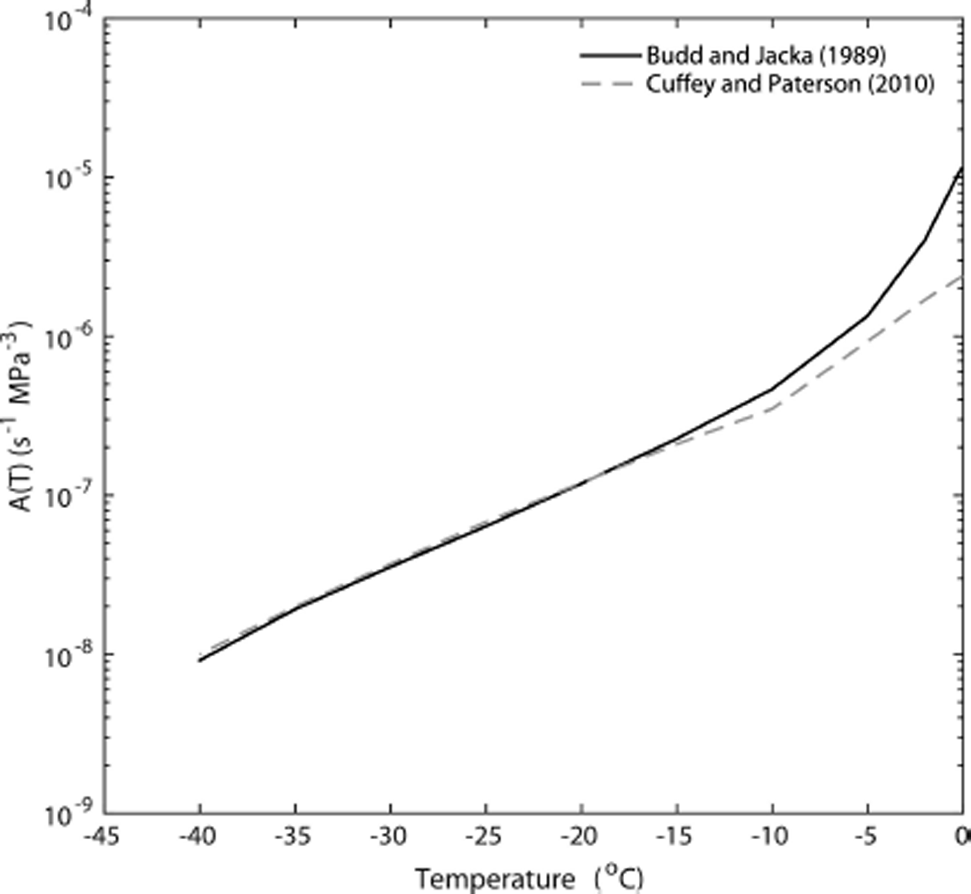
The A(T) values of Reference Cuffey and PatersonCuffey and Paterson (2010) are presented in Figure 3 for comparison with the values derived from the Reference Budd and JackaBudd and Jacka (1989) data. Over the temperature range in the DSS borehole of −21.8°C to −6.9°C the Reference Budd and JackaBudd and Jacka (1989) values are largely similar to those of Reference Cuffey and PatersonCuffey and Paterson (2010); however, above −15°C the Reference Budd and JackaBudd and Jacka (1989) derived values are more sensitive to increasing temperature, leading to higher values, particularly above −10°C.

In addition to A(T) values determined using the Reference Budd and JackaBudd and Jacka (1989) data, the TNNI flow relation, Eqn (18), is calibrated using the dimensionless parameter, B, to provide physically reasonable strain-rate (or stress) estimates (Eqns (15) and (16)). For strain rates calculated using a statistically isotropic distribution of N _T ≈ 8.5 × 10⁴ c-axes, the value of B required for strain rates to match the Reference Budd and JackaBudd and Jacka (1989) secondary (minimum) creep values varies according to the specified level of neighbour grain interaction, i.e. with the grain interaction parameters, C ₀ and C _n. Reference ThorsteinssonThorsteinsson (2001) provides an analytically derived value of B = 630 for homogeneous stress conditions with no neighbour grain interactions (e.g. C ₀ = 1 and C _n = 0), whilst for the case of full neighbour grain interaction, (C ₀ = 1; C _n = 1), we find B = 565.

In the derivation of the AGA flow relation, Reference Azuma and Goto-AzumaAzuma and Goto-Azuma (1996) used the temperature-dependent flow parameter, β_S , specific to single-crystal deformation (Eqn (10)). For an isotropic distribution of c-axes this leads to strain rates three to four orders of magnitude higher than observed polycrystalline strain rates under similar conditions of temperature and stress (Reference TreverrowTreverrow, 2009). To correct this discrepancy we calibrate the AGA relation using a procedure similar to that for the TNNI relation. Using the same statistically isotropic distribution of N _T ≈ 8.5 × 10⁴ c-axes and the Reference Budd and JackaBudd and Jacka (1989) A(T), a scaling parameter is determined so that the isotropic strain rates match the Reference Budd and JackaBudd and Jacka (1989) secondary creep rates.

Sensitivity of flow relations to fabric data array size

The parameterization of crystal orientation fabrics using an ODF may not adequately describe distributions where the number of c-axis orientations is <100. When implementing the flow relations to determine borehole stress profiles, we solve AGA, TNNI and CAFFE numerically, with discrete summations over the measured c-axis orientation data. This avoids any loss of fabric detail through conversion to a restrictive form of ODF.

Figure 4 illustrates how uncertainty in AGA, TNNI and CAFFE strain-rate predictions varies with the number of c-axis vectors in an isotropic fabric created by random selection from a simulated isotropic distribution of 8.5 × 10⁴ axes. Normalized strain rates were calculated for simple shear on isotropic fabrics with N = 50 to 1.0 × 10⁴ c-axes. For each N, 50 simulated fabrics were randomly selected from the original distribution and their normalized strain rates calculated. In each case the reference strain rates for normalization were calculated using the same isotropic distribution of 8.5 × 10⁴ axes. These rates are equivalent to the analytically derived rates for an ideal isotropic distribution. For fabrics described by an array of c-axis vectors it is possible for the AGA and TNNI flow relations to predict components where there is no corresponding S_ij component. To incorporate the influence of this effect on the overall deformation, all normalized strain rates (Fig. 4) are calculated using octahedral shear strain rates.

Fig. 4. Variability in normalized octahedral shear strain rates as a function of N, the number of c-axes in simulated isotropic crystal orientation fabrics. Strain rates are for the (a) AGA, (b) TNNI and (c) CAFFE flow relations. For each value of N the mean and standard deviation of the octahedral shear strain rate were calculated for 50 simulated fabrics randomly selected from the same isotropic distribution of 8.5 × 10⁴ axes. Strain rates calculated for each flow relation were normalized against rates determined using the reference isotropic fabric of 8.5 × 10⁴ axes. Results for the TNNI flow relation were calculated with full neighbour grain interaction and CAFFE rates were calculated using E _max = 8.

The uncertainty in strain rates predicted using the AGA, CAFFE and TNNI flow relations is highest for low-N fabrics due to the greater potential for individual grains, with a high degree of misorientation relative to the mean orientation, to influence the bulk strain rates. The values presented for isotropic fabrics (Fig. 4) represent an upper limit of c-axis orientation-based uncertainty in strain rates for each N. As fabrics become increasingly anisotropic the mean misorientation of c-axes decreases, reducing the potential for any individual grains to strongly influence the bulk strain rates. In this study we use fabric data measurements that predate modern automated ice crystal fabric analysers, so individual fabrics are restricted to N ≈ 100 orientations due to the arduous nature of conducting multiple Rigsby stage analyses (Fig. 2c). For anisotropic fabrics, measurement of N ≈ 80–100 c-axes is adequate to describe the distribution (e.g. Reference Durand, Gagliardini, Thorsteinsson, Svensson, Kipfstuhl and Dahl-JensenDurand and others, 2006; Reference Gow and MeeseGow and Meese, 2007); however, this value increases as fabrics become increasingly isotropic.

To minimize uncertainty in the flow relation stress estimates based on fabrics with N < 100, composite fabrics have been created by combining five sequential fabrics, resulting in N ≈ 500. This smooths the fabric data over an interval of ∼25–40 m (bold lines in Fig. 2c). The depth assigned to each of the 185 composites is the moving mean of the five contributing fabric depths. With this technique the number of individual fabrics contributing to the composites is lower for the uppermost and lowermost two cases, which are derived from three and four members respectively.

Flow configuration at DSS

From surface and borehole strain-rate observations (Reference Morgan, Van Ommen, Elcheikh and LiMorgan and others, 1998) the flow configuration at the DSS site is assumed to be horizontal simple shear parallel to the surface flow direction, combined with extension both parallel and transverse to the flow direction. This flow configuration corresponds to that specified for the B2013 flow relation in Eqn (25). The ζ parameter describing the relative proportions of the normal flow components can be determined from the ratio of the GPS-determined surface strain-rate components, i.e. (Table 1), leading to and

(28)

so that vertical profiles of and can be obtained from the profile. The agreement between the surface value of the vertical strain-rate profile, (Eqns (3) and (4)) and the GPS-determined (Reference Morgan, Van Ommen, Elcheikh and LiMorgan and others, 1998) provides validation of the borehole inclination derived profile.

Procedures for estimating stress profiles

The procedures used to estimate S_xz and S_zz profiles using the available strain-rate, temperature and crystal orientation data vary for each flow relation. We calculate the vertical deviator, S_zz , since links more directly to the calculated profile (Eqn (3)). In all cases a stress configuration of the form

(29)

is assumed where is used. The borehole strain-rate and temperature data (Fig. 2) are available at higher spatial resolution than the fabric data, so values corresponding to the composite fabric depths were determined by interpolation.

Owing to the collinear relationship between and S components in the B2013 flow relation, at each depth interval . From the depth profile of , substitution of into Eqns (26) and (27) gives

(30)

from which S_zz is easily obtained.

For the CAFFE flow relation S_xz and S_zz are calculated using the composite fabric data appropriate to each depth (Eqns (21) and (23)).

For the AGA and TNNI flow relations a tensor relationship exists between and S , necessitating indirect calculation of stress profiles via a more complex two-step process. Firstly, temperature-independent values were calculated for each fabric using S (Eqn (29)), where the proportions of S_xz and S_zz were varied iteratively for values of a shear stress parameter (Reference Warner, Jacka, Li, Budd, Hutter, Wang and BeerWarner and others, 1999),

(31)

where 0 ≤ r _s ≤ 1. The shear parameter r _s = 0 when S_xz = 0, and r _s = 1 when S_zz = 0. When S_xz = S_zz (equal deviators) r _s = 0.5. For each composite fabric the r_s value that produces the strain-rate ratio, , which matches the borehole-derived value for that depth was determined. In this step, only the relative proportions of S_xz and S_zz are required since is a function of the fabric and r _s, i.e. their magnitudes and the temperature dependence are unimportant, only their relative proportion matters. Secondly, was recalculated for each composite fabric using the appropriate A(T) value (Eqn (16)), for the corresponding depth. For each fabric the magnitudes of S_xz and S_zz were varied iteratively, according to the proportions described by the corresponding r _s value, until the correct borehole and values were reproduced.

Comparison with observations from laboratory ice-deformation experiments

While prediction of S_xz and S_zz profiles using ice-core and borehole data allows differentiation of the flow relations based on their description of anisotropic rheology, such a comparison does not provide an assessment of whether or not the relative proportions of the stress tensor components are physically realistic. In the following we use data from laboratory ice deformation experiments to support our analysis of the AGA, TNNI, CAFFE and B2013 flow relations.

In experiments on laboratory-made ice conducted in combined simple shear and confined vertical compression stress configurations, with different proportions of S_xz and S_zz , Reference Li, Jacka and BuddLi and others (1996) and Reference Budd, Warner, Jacka, Li and TreverrowBudd and others (2013) demonstrated that during tertiary creep all strain-rate components were enhanced relative to the expectations from the Reference GlenGlen (1958) flow relation. In particular the compression rates were enhanced, even as the shear stress proportion increased and became dominant. Furthermore, this enhancement occurs despite the development of compatible fabric patterns that might be considered to contain a high proportion of hard-glide c-axis orientations with respect to the compressive deviatoric stress component. The general similarity of the DSS-site flow configuration and that of the experiments of Reference Li, Jacka and BuddLi and others (1996) and Reference Budd, Warner, Jacka, Li and TreverrowBudd and others (2013) allows for a comparison of DSS- and experimentally based flow relation predictions.

Strain-rate and c-axis orientation data from two experiments in the series of Reference Budd, Warner, Jacka, Li and TreverrowBudd and others (2013), and another conducted using the same apparatus and experimental techniques as Reference Budd, Warner, Jacka, Li and TreverrowBudd and others (2013), were used to calculate the ratio of the simple shear and confined compression deviatoric stresses, S_xz /S_zz . In Table 2 these values are compared to the applied experimental stresses. We examine cases where the applied ratios of deviatoric stresses were S_xz /S_zz = 0.5, 1.0 and 2.0. The corresponding strain-rate ratios for these experiments were , 1.05 and 1.59, respectively (Table 2). These values are generally consistent with a collinear relationship between the components of and S : the ≤20% difference between the stress and strain-rate component ratios is within the 95% confidence interval for the variability between replicate experiments (Reference Treverrow, Budd, Jacka and WarnerTreverrow and others, 2012).

Table 2. The ratio of simple shear and vertical compression deviatoric stress tensor components calculated using experimental tertiary creep rate and c-axis orientation fabric data. The initially isotropic polycrystalline ice samples were deformed in combined stress configurations incorporating various proportions of simple shear and confined vertical compression. All experiments were conducted at −2°C. Experimental data for (b) and (c) are from Reference Budd, Warner, Jacka, Li and TreverrowBudd and others (2013) (table 1, experiments 22 and 24, respectively). The data for (a) were obtained using the same apparatus and experimental techniques as Reference Budd, Warner, Jacka, Li and TreverrowBudd and others (2013). (a) Compression-dominated with S_xz /S_zz = 0.50, S_xz = 0.219 MPa and τ _o = 0.40 MPa. (b) Equal shear and compression deviators, S_xz /S_zz = 1.0, S_xz = 0.49 MPa and τ _o = 0.57 MPa. (c) Shear-dominated with with S_xz /S_zz = 2.0, S_xz = 0.49 MPa and τ _o = 0.45 MPa. The experimental stress configuration is defined by a Cartesian coordinate system where the x-axis is the shear direction and the z-axis is normal to the plane of the page. The crystal orientation data are presented in lower-hemisphere Schmidt plots aligned with the xy-plane

Due to the collinearity of the B2013 and CAFFE flow relations the stress ratios calculated for the experiments are precisely the strain-rate component ratios. Thus, for the experiments where S_xz /S_zz = 1.0 and 2.0 the B2013 and CAFFE relations return S_xz /S_zz = 1.05 and 1.59 (cf. the corresponding strain-rate ratios of and 1.59, respectively, in Table 2). In contrast the AGA and TNNI relations predict significantly lower S_xz /S_zz ratios that are only 40–49% of the B2013/CAFFE values. These low AGA and TNNI S_xz /S_zz values in flow configurations where S_xz ≥ S_zz are consistent with the presented DSS borehole analysis. Figure 5 demonstrates how the four anisotropic flow relations predict similar S_xz values using the DSS borehole and ice-core data: it is the marked variability in their S_zz predictions that drives differences in the S_xz /S_zz ratio. Therefore, the S_xz /S_zz values predicted by the AGA and TNNI relations are inconsistent with tertiary creep observations from combined simple shear and confined vertical compression experiments where .

For the compression-dominated experiment, where S_xz /S_zz = 0.5 (Table 2), the predictions of the AGA and TNNI flow relations correspond more closely to the experimental observations and the B2013 and CAFFE relations. This improved performance is related to the generally decreasing strength of the c-axis fabrics in these flow configurations. The weakly clustered fabric for the experiment where S_xz /S_zz = 0.5 exhibits a low level of compatibility with both the simple shear and confined compression components. For the AGA and TNNI flow relations this results in moderate enhancement of both strain-rate components and predicted stress ratios that agrees well with the expected value of S_xz /S_zz = 0.5.

As the experiments become increasingly shear-dominated, i.e. where S_xz ≥ S_zz , the fabrics evolve towards distributions containing a higher proportion of near-vertical c-axes. The very low vertical compressive stress components resolved on the basal planes of grains with near-vertical c-axes drive the high S_zz values that are necessary to reproduce the experimental observations.

This assessment of the flow relations using experimental data is consistent with the analysis based on DSS borehole and ice-core data. For each experiment in Table 2, we identify the DSS borehole depths where the derived strain-rate ratios, , are equivalent to the experimental values. As was found for the stress ratios calculated using experimental data, the DSS borehole S_xz /S_zz values, at the specific depths corresponding to the experiment-based simulations, indicate how the AGA and TNNI flow relations consistently overestimate S_zz , particularly where .

While data from the combined stress experiments necessary to investigate the collinearity of flow relations are currently sparse (e.g. Reference Li, Jacka and BuddLi and others, 1996; Reference Budd, Warner, Jacka, Li and TreverrowBudd and others, 2013), we are not aware of any data that support the low S_xz /S_zz values predicted by the AGA and TNNI flow relations in complex stress configurations where the flow is shear-dominated. Further laboratory studies to investigate these combined-stress configuration effects are ongoing. More generally, this study demonstrates the difficulties associated with the development of flow relations based on a grain-scale description of deformation and recovery processes: unless all processes important to the flow are adequately described, the prescribed rheology will be incomplete and potentially unrealistic.

Future flow relation developments

A primary consideration in the development of flow relations for ice-sheet modelling is to minimize the computational cost while improving the representation of anisotropic rheology. The CAFFE and B2013 flow relations are based on parameterizations of key rheological variables with resultant low computational overhead and, particularly for B2013, have relatively straightforward requirements for implementation within ice-sheet models. Of the flow relations investigated here, the CAFFE and B2013 flow relations provide the most physically realistic predictions of deviatoric stresses at the DSS site, despite their relative simplicity.

While the CAFFE flow relation has been implemented in the 3-D FEM full-Stokes ice-sheet model Elmer/Ice (Reference GagliardiniGagliardini and others, 2013), to investigate regional ice-sheet dynamics around deep ice-core drilling sites (Reference Seddik, Greve, Placidi, Hamann and GagliardiniSeddik and others, 2008) the computational cost and complexity of a scheme describing the spatial and temporal evolution of crystal orientation fabrics so far prohibit its application in long-term continental-scale simulations.

The anisotropy of the B2013 flow relation (Eqn (27)) is determined from the relative proportions of the deviatoric stress (or strain-rate) components, eliminating the requirement to simulate fabric evolution in forward modelling. The B2013 flow relation is based on data from laboratory deformation experiments conducted in stress configurations incorporating specific combinations of simple shear and vertical compression. While these stress configurations are relevant to describing the flow regime at DSS, a generalized form of the B2013 flow relation, as described by Reference Budd, Warner, Jacka, Li and TreverrowBudd and others (2013), is required for large-scale dynamic simulations where a wider range of stress configurations is encountered.

The physically motivated descriptions of intra- and intercrystalline deformation and recovery processes in the AGA and TNNI flow relations lead to complex rheologies with tensor descriptions of viscosity. Whilst some full-Stokes models provide the necessary framework to support anisotropic tensor viscosities, the additional complexity of the AGA and TNNI flow relations, including the requirement to simulate fabric evolution, precludes their application in continental-scale ice-sheet models. Application of the TNNI relation is further restricted by the explicit inclusion of nearest-neighbour grain interactions. Rather than being directly applied in ice-sheet models the future benefit of such physically motivated flow relations lies in their value as tools to improve understanding of intra- and intercrystalline deformation and recrystallization processes (e.g. Reference LlorensLlorens and others, 2014; Reference MontagnatMontagnat and others, 2014b). The identification of commonalities in the microstructure and deformation processes observed in laboratory and ice-core samples, in conjunction with microstructure modelling, will support the development of phenomenological flow relations for ice-sheet modelling, and their extrapolation to a broader range of temperature and stress conditions than can be readily achieved in laboratory studies.

The continued development of anisotropic flow relations for ice-sheet modelling relies on the availability of laboratory, field and remotely sensed observations of ice dynamics. In general, reliable experimental data for flow relation development are sparse, with tertiary creep observations even more limited. Additional statistically robust strain-rate data and microstructural observations are required to extend the range of stress configurations, magnitudes and temperatures over which an improved anisotropic flow relation can be reliably specified. For example, a creep power law stress exponent of n = 3 in Eqn (1) is well established for secondary (isotropic minimum) strain rates. Analysis by Reference Treverrow, Budd, Jacka and WarnerTreverrow and others (2012) of the limited available tertiary creep data from shear alone and compression alone experiments suggests a stress exponent of n = 3.5 may be appropriate for describing tertiary creep, at least for some stress configurations (and possibly stress magnitudes; e.g. Reference PettitPettit and others (2011) discuss the transition to a flow regime with n = 1 at low stresses). In the context of a Glen-type flow relation, a stress exponent of n = 3.5 may be paramaterized by a stress-dependent enhancement factor, , where

(33)

Further experimental data are required to validate this effect over a wider range of stress configurations and temperatures. Prescription of a stress-dependent enhancement term to accommodate a flow relation where n = 3.5 would be straightforward for the CAFFE and B2013 flow relations, and others with an experimentally derived scalar enhancement term (e.g. Reference Pettit, Thorsteinsson, Jacobson and WaddingtonPettit and others, 2007).