


1. Introduction
The concept of a Dialogue Act (DA) originated from John Austin’s ‘illocutionary act’ theory (Austin Reference Austin1962) and was later developed by John Searle (Reference Searle1969), as a method of defining the semantic content and communicative function of a single utterance of dialogue. The fields of Natural Language Processing (NLP) and Natural Language Understanding (NLU) have since developed many applications for the automatic identification, or classification, of DA’s. Most prominently, within dialogue management systems, they have been used as high-level representations for user intents, system actions and dialogue state (Griol et al. Reference Griol, Hurtado, Segarra and Sanchis2008; Ge and Xu Reference Ge and Xu2015; CuayÁhuitl et al. Reference Cuayáhuitl, Yu, Williamson and Carse2016; Wen et al. Reference Wen, Gašić, Mrkšić, Rojas-Barahona, Su, Ultes, Vandyke and Young2016; Liu et al. Reference Liu, Tur, Hakkani-Tur, Shah and Heck2018; Firdaus et al. Reference Firdaus, Golchha, Ekbal and Bhattacharyya2020). DA’s have also been applied to spoken language translation (Reithinger et al. Reference Reithinger, Engel, Kipp and Klesen1996; Kumar et al. Reference Kumar, Agarwal, Dasgupta, Joshi and Kumar2017), team communication in the domain of robot-assisted disaster response (Anikina and Kruijff-Korbayova Reference Anikina and Kruijff-Korbayova2019) and understanding the flow of conversation within therapy sessions (Lee et al. Reference Lee, Hull, Levine, Ray and McKeown2019). However, the DA classification task has yet to reach, or surpass, the human level of performance that has been achieved for many other NLP tasks and thus remains an open and interesting area of research.
Previous approaches to the DA classification task include support vector machines (SVM) (Ribeiro et al. Reference Ribeiro, Ribeiro and Martins De Matos2015; Amanova et al. Reference Amanova, Petukhova and Klakow2016), and hidden Markov models (HMM) (Stolcke et al. Reference Stolcke, Ries, Coccaro, Shriberg, Bates, Jurafsky, Taylor, Martin, Van Ess-Dykema and Meteer2000; Surendran and Levow Reference Surendran and Levow2006), N-grams (Louwerse and Crossley Reference Louwerse and Crossley2006) and Bayesian networks (Keizer Reference Keizer2001; Grau et al. Reference Grau, Sanchis, Castro and Vilar2004). Though, more recently, performance of deep learning techniques, often based on recurrent or convolutional architectures, have surpassed that of the more traditional approaches previously mentioned (Kalchbrenner and Blunsom Reference Kalchbrenner and Blunsom2013; Ji et al. Reference Ji, Haffari and Eisenstein2016; Lee and Dernoncourt Reference Lee and Dernoncourt2016; Papalampidi et al. Reference Papalampidi, Iosif and Potamianos2017). Regardless of architectural variations, such neural network models may be broadly split into two categories, referred to here as single-sentence and contextual. Single-sentence models take one utterance of dialogue as input and assign a predicted DA label for that utterance. On the other hand, input for contextual models includes additional historical or contextual information, for example, indicating a change in speaker, previous dialogue utterances or previously predicted DA labels. In some cases, the contextual information may also include ‘future’ utterances or DA labels, in other words, those that appear after the current utterance requiring classification; though, the utility of such future information for real-time applications such as dialogue systems is questionable. Within DA classification research, it has been widely shown that including such contextual information yields improved performance over single-sentence approaches (Lee and Dernoncourt Reference Lee and Dernoncourt2016; Liu and Lane Reference Liu and Lane2017; Bothe et al. Reference Bothe, Magg, Weber and Wermter2018a; Ribeiro et al. Reference Ribeiro, Ribeiro and De Matos2019). The advantage of including contextual information is clear when considering the nature of dialogue as a sequence of utterances. Often, utterances are not produced independently of one another, instead they are produced in response to previous talk. Consider the use of ‘Okay’ in the following examples. In the first instance, speaker B uses ‘Okay’ in response to a question. In the second instance, speaker A uses ‘Okay’ as confirmation that a response has been heard and understood. As such, it may be difficult, or impossible, to determine the communicative intent of a single-dialogue utterance and, therefore, including contextual information results in superior performance over single-sentence approaches.

Consequently, much of the contemporary DA classification research focused on representing contextual information and related architectures. Yet, both single-sentence and contextual classification models share some commonalities. Primarily, that is, each input utterance, or utterances, must first be encoded into a format conducive to classification, most commonly with several feed forward neural network (FFNN) layers, or further downstream operations, such as combining additional contextual information (Kalchbrenner and Blunsom Reference Kalchbrenner and Blunsom2013; Lee and Dernoncourt Reference Lee and Dernoncourt2016; Ortega and Vu Reference Ortega and Vu2017; Papalampidi et al. Reference Papalampidi, Iosif and Potamianos2017; Bothe et al. Reference Bothe, Weber, Magg and Wermter2018b). In other words, the plain text input utterances must be converted into a vector representation that ‘encodes’ the semantics of the given utterance. It is this sentence encoding module which is common to most DA classification approaches. However, in our experience, much of the previous work on DA classification has neglected to examine the impact of input sequence representations on sentence encoding, for example, the number of words permitted in the vocabulary, the number of tokens within an input sequence, the selection of pre-trained word embeddings, and so on. Where such considerations are reported, they are often brief and with little justification as to their efficacy. Further, their effect on results may be difficult to determine when most work focuses on one, or a small number of, sentence encoding models. Here, we instead elect to examine factors which may, or may not, contribute to effective encodings of single-dialogue utterances.
In this study, we conduct a comprehensive investigation of several key components that contribute to the sentence encoding process. The hypothesis being, that if we can determine the elements which contribute to effective DA classification at the single-sentence level, then they may also be applied at the contextual level. We analyse the effect of different parameters for input sequence representations on a number of supervised sentence encoder models, based on a mixture of recurrent and convolutional architectures. Further, given the recent successes of using large pre-trained language models for transfer learning on a variety of NLP tasks, including those based on the Transformer architecture (Vaswani et al. Reference Vaswani, Shazeer, Parmar, Uszkoreit, Jones, Gomez, Kaiser and Polosukhin2017), such as BERT (Devlin et al. Reference Devlin, Chang, Lee and Toutanova2019) and GPT2 (Radford et al. Reference Radford, Wu, Child, Luan, Amodei and Sutskever2019), we test a number of such models as sentence encoders for the, as yet largely unexplored, task of DA classification. This work should also serve as a useful reference for future research on the DA classification task, by providing some empirical data regarding various implementation decisions.
In the following section, we provide an overview of the sentence encoding and DA classification process, with particular focus on the aspects explored within this work, including the different features of input sequence representations and pre-trained embeddings, supervised encoder models, and pre-trained language models. Section 3 describes our experimental set-up, including the two corpora used for training and evaluation within the study, along with an explanation of the text pre-processing procedure and selection of training and test data, implementation details of the supervised and pre-trained language models used throughout the experiments, and our evaluation procedure. In Section 4, we report the results we obtain for our input sequence experiments, using supervised models, and the language model experiments. Final discussion and conclusions are drawn in Section 5Footnote a.
2. Sentence encoding and DA classification
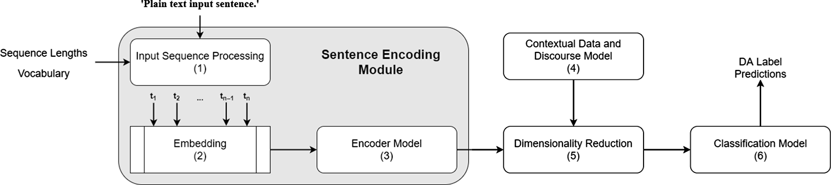
In this section, we describe the various components of sentence encoding process, with respect to the DA classification task, and provide details of each aspect investigated in this work. Both single-sentence and contextual models tend to share a common sentence encoding module. Though specific implementation details may vary, most may be described with the generic DA classification architecture diagram shown in Figure 1. The sentence encoding module encompasses several components, each of which is examined within this study. In short, the encoding module converts the plain text input sentences into the vectorised representations necessary for classification or other downstream tasks, such as concatenation with other contextual data. The following sections discuss each component of Figure 1 (numbered 1 through 6) in more detail.
A generic DA classification architecture, including the sentence encoding module (components 1-3), and example parameters (Sequence Length, Vocabulary, etc), additional context information (4), dimensionality reduction (5) and classification (6).
2.1 Input sequence processing
The input sequence processing component (1) takes as input a plain text sentence and produces a tokenised sequence. Generally, this procedure is carried out as part of pre-processing the data prior to training, or inference. Sequence processing involves several text pre-processing steps and, as previously mentioned, they are often only briefly reported within the literature, if at all. Where they are, the selected parameters are rarely justified and therefore appear somewhat arbitrarily chosen in many cases. Additionally, very few studies have explored the impact that different parameters may have on the resulting sentence encodings. Here, we discuss three different, in some cases optional, aspects of the sequence processing component: letter case and punctuation, vocabulary size, and tokenisation.
2.1.1 Letter case and punctuation
Letter case simply refers to the optional pre-processing step of converting the letters in all words to lower case, or not, which helps to reduce ‘noise’ within the data. Firstly, by reducing repeated words in the vocabulary, for example, removing words that are capitalised at the beginning of a sentence and appear lower-cased elsewhere, and secondly, by removing capitals from names, abbreviations, and so on. Converting all words to lower case is common practice in many NLP applications and the same appears true for DA classification (Ji et al. Reference Ji, Haffari and Eisenstein2016; Kumar et al. Reference Kumar, Agarwal, Dasgupta, Joshi and Kumar2017; Chen et al. Reference Chen, Yang, Zhao, Cai and He2018; Wan et al. Reference Wan, Yan, Gao, Zhao, Wu and Yu2018), though, it is often not stated whether this step has been carried out.
Whether to remove punctuation, or not, is another optional pre-processing step. It seems reasonable to assume that, for the DA classification task, some punctuation marks may contain valuable information which should not be removed. Certainly, an interrogation mark at the end of a sentence should indicate a high probability that it was a question. For instance, Wan et al. (Reference Wan, Yan, Gao, Zhao, Wu and Yu2018) removed all punctuation marks except for interrogation, and Kumar et al. (Reference Kumar, Agarwal, Dasgupta, Joshi and Kumar2017) removed only exclamation marks and commas. On the other hand, Webb and Hepple (Reference Webb and Hepple2005) removed all punctuation, though none of these studies states why those particular choices were made. However, Ortega et al. (Reference Ortega, Li, Vallejo, Pavel and Vu2019) found that keeping punctuation was beneficial on a similar DA classification task using the Meeting Recorder Dialogue Act (MRDA) dataset, and it is therefore worthy of further investigation.
In addition to case and punctuation, lemmatising words or converting them to their parts of speech (POS) is a frequently used pre-processing step within NLP applications. However, previous studies have shown that, whether used as additional features (Kumar et al. Reference Kumar, Agarwal, Dasgupta, Joshi and Kumar2017), or replacing words entirely (Ribeiro et al. Reference Ribeiro, Ribeiro and De Matos2019), they result in an unfavourable effect on performance. We therefore chose to focus solely on letter case and punctuation within this study (see Section 4.1.1).
2.1.2 Vocabulary size
Corpora often contain a large number of unique words within their vocabulary. It is common practice, within NLP and DA classification tasks, to remove words that appear less frequently within the corpus. Or in other words, to keep only a certain number – the vocabulary size – of the most frequent words and consider the rest out-of-vocabulary (OOV), which are often replaced with a special ‘unknown’ token, such as <unk> (Ji et al. Reference Ji, Haffari and Eisenstein2016; Wan et al. Reference Wan, Yan, Gao, Zhao, Wu and Yu2018). Though a vocabulary size is often stated within DA classification studies, it is generally not accompanied with an explanation of why that value was chosen. For example, the Switchboard corpus contains ${\sim}{22,000}$
unique words (this varies depending on certain pre-processing decisions, see Section 3.1), yet different studies have elected to use vocabulary sizes in the range of 10,000 to 20,000 words (Ji et al. Reference Ji, Haffari and Eisenstein2016; Lee and Dernoncourt Reference Lee and Dernoncourt2016; Kumar et al. Reference Kumar, Agarwal, Dasgupta, Joshi and Kumar2017; Li et al. Reference Li, Lin, Collinson, Li and Chen2018; Chen et al. Reference Chen, Yang, Zhao, Cai and He2018), while Wan et al. (Reference Wan, Yan, Gao, Zhao, Wu and Yu2018) kept only words that appeared more than once within the corpus. To the best of our knowledge, only one previous study has explored the effect of different vocabulary sizes on DA classification task. Cerisara et al. (Reference Cerisara, KrÁl and Lenc2017) conducted experiments on the Switchboard corpus using different vocabulary sizes in the range 500 to 10,000. They found that, with their model, the best performance was achieved with a vocabulary size of between 1,000 and 2,000 words and that accuracy slightly decreased with larger vocabularies. This indicates that the choice of vocabulary size may well impact the DA classification task. As such, we evaluate the effect on performance of a range of vocabulary sizes (see Section 4.1.2).
${\sim}{22,000}$
unique words (this varies depending on certain pre-processing decisions, see Section 3.1), yet different studies have elected to use vocabulary sizes in the range of 10,000 to 20,000 words (Ji et al. Reference Ji, Haffari and Eisenstein2016; Lee and Dernoncourt Reference Lee and Dernoncourt2016; Kumar et al. Reference Kumar, Agarwal, Dasgupta, Joshi and Kumar2017; Li et al. Reference Li, Lin, Collinson, Li and Chen2018; Chen et al. Reference Chen, Yang, Zhao, Cai and He2018), while Wan et al. (Reference Wan, Yan, Gao, Zhao, Wu and Yu2018) kept only words that appeared more than once within the corpus. To the best of our knowledge, only one previous study has explored the effect of different vocabulary sizes on DA classification task. Cerisara et al. (Reference Cerisara, KrÁl and Lenc2017) conducted experiments on the Switchboard corpus using different vocabulary sizes in the range 500 to 10,000. They found that, with their model, the best performance was achieved with a vocabulary size of between 1,000 and 2,000 words and that accuracy slightly decreased with larger vocabularies. This indicates that the choice of vocabulary size may well impact the DA classification task. As such, we evaluate the effect on performance of a range of vocabulary sizes (see Section 4.1.2).
2.1.3 Tokenisation
The final stage of preparing the input sequence is that of transforming the plain text sentence into a fixed length sequence of word or character tokens. Tokenisation at the word level is the most common approach for DA classification because it enables the mapping of words to pre-trained embeddings and hence facilitates transfer learning. Though, recently some studies have also explored character-based language models (Bothe et al. Reference Bothe, Weber, Magg and Wermter2018b), or a combination of character and word embeddings (Ribeiro et al. Reference Ribeiro, Ribeiro and De Matos2019). In any case, once the text has been tokenised, it is padded or truncated to a fixed size sequence length, or maximum sequence length. In cases where the number of tokens is less than the maximum sequence length, extra ‘padding’ tokens, such as <pad>, are used to extend the sequence to the desired size. Input sequences must be converted to a fixed length because many sentence encoding, and classification, models require the size of the input data to be defined before runtime, or before processing a batch of data, for example, to determine the number of iterations over the input sequence for recurrent models. The final tokenisation step is to simply map each word, or character, to an integer representation. In the case of word tokens, this is typically the words index within the vocabulary.
Choosing a sequence length equal to the number of tokens in the longest sentence in the corpus may result in the majority of sequences consisting predominantly of the padding token, and hence, increasing the computational effort without adding any useful information. For instance, the Switchboard corpus has an average of ${\sim}9.6$
tokens per utterance, yet the maximum utterance length is 133 tokens. On the other hand, if an input sequence is too short, the process of truncation could remove information valuable to the encoding and classification process. However, considerations around appropriate values for input sequence length are rarely discussed within the literature. To the best of our knowledge, thus far only two studies have explored the impact of different sequence lengths on the DA classification task. Cerisara et al. (Reference Cerisara, KrÁl and Lenc2017) tested different sequence lengths in the range 5 to 30 on the Switchboard corpus. They found the best performance was achieved using 15 to 20 tokens, with further increases not yielding any improvement. Similarly, Wan et al. (Reference Wan, Yan, Gao, Zhao, Wu and Yu2018), using the same corpus, tested sequence lengths in the range 10 to 80 and achieved their best results with a sequence length of 40, with further increases actually reducing performance. These results suggest that, as with vocabulary size, the value selected for maximum sequence length is also worth further investigation. We therefore evaluate the impact of different sequence lengths on classification results (see Section 4.1.3).
${\sim}9.6$
tokens per utterance, yet the maximum utterance length is 133 tokens. On the other hand, if an input sequence is too short, the process of truncation could remove information valuable to the encoding and classification process. However, considerations around appropriate values for input sequence length are rarely discussed within the literature. To the best of our knowledge, thus far only two studies have explored the impact of different sequence lengths on the DA classification task. Cerisara et al. (Reference Cerisara, KrÁl and Lenc2017) tested different sequence lengths in the range 5 to 30 on the Switchboard corpus. They found the best performance was achieved using 15 to 20 tokens, with further increases not yielding any improvement. Similarly, Wan et al. (Reference Wan, Yan, Gao, Zhao, Wu and Yu2018), using the same corpus, tested sequence lengths in the range 10 to 80 and achieved their best results with a sequence length of 40, with further increases actually reducing performance. These results suggest that, as with vocabulary size, the value selected for maximum sequence length is also worth further investigation. We therefore evaluate the impact of different sequence lengths on classification results (see Section 4.1.3).
2.2 Embeddings
The embedding component (2) is often the first layer of a DA classification model. Though, this is typically not the case with many pre-trained language models, where input is simply the tokenised sentence (see Section 2.3.2). The embedding layer maps each word in the tokenised input sequences to higher-dimensional vector representations, most frequently with pre-trained embeddings such as Word2Vec (Mikolov et al. Reference Mikolov, Yih and Zweig2013) and GloVe (Pennington et al. Reference Pennington, Socher and Manning2014).
However, within the literature, a number of studies simply state the type and dimensions of the embeddings used (Lee and Dernoncourt Reference Lee and Dernoncourt2016; Ortega and Vu Reference Ortega and Vu2017; Li et al. Reference Li, Lin, Collinson, Li and Chen2018; Ahmadvand et al. Reference Ahmadvand, Choi and Agichtein2019), while others have explored several different types or dimensions (Cerisara et al. Reference Cerisara, KrÁl and Lenc2017; Papalampidi et al. Reference Papalampidi, Iosif and Potamianos2017). Ribeiro et al. (Reference Ribeiro, Ribeiro and De Matos2019) examined a number of 300-dimensional pre-trained embeddings: Word2Vec (Mikolov et al. Reference Mikolov, Yih and Zweig2013), FastText (Joulin et al. Reference Joulin, Grave, Bojanowski and Mikolov2017) and Dependency (Levy and Goldberg Reference Levy and Goldberg2014), with the latter yielding the best results. In contrast, it appears 200 to 300-dimensional GloVe embeddings (Pennington et al. Reference Pennington, Socher and Manning2014) are used more frequently within DA classification studies (Lee and Dernoncourt Reference Lee and Dernoncourt2016; Kumar et al. Reference Kumar, Agarwal, Dasgupta, Joshi and Kumar2017; Papalampidi et al. Reference Papalampidi, Iosif and Potamianos2017; Chen et al. Reference Chen, Yang, Zhao, Cai and He2018; Li et al. Reference Li, Lin, Collinson, Li and Chen2018; Wan et al. Reference Wan, Yan, Gao, Zhao, Wu and Yu2018). As such, it is difficult to determine whether any one type of pre-trained embedding, or its dimensionality, is optimal for the DA classification task. Additionally, it is unclear what impact different embedding and dimensionality choices may have on classification results. As an example, according to the results reported by Ribeiro et al. (Reference Ribeiro, Ribeiro and De Matos2019), the difference between their best- and worst-performing pre-trained embeddings, Dependency and FastText, respectively, is 0.66%. While the difference between FastText and Word2Vec was only 0.2%. Therefore, we examine five different pre-trained embeddings and test each at five different dimensions in the range 100 to 300 (see Section 4.2).
It should be noted that, to the best of our knowledge, no embeddings have been developed specifically for the DA classification task. Word embeddings are typically trained on large amounts of text data, for example, Word2Vec was developed using a 1.6 billion word dataset (Mikolov et al. Reference Mikolov, Yih and Zweig2013). Thus, developing embeddings for DA classification, either from scratch, or by fine-tuning existing embeddings, would likely require a very large set of dialogue data. Though this would be an interesting avenue to pursue, here we chose to focus our experiments on existing embeddings, as these are the most frequently used, and leave DA-oriented embeddings for future research.
2.3 Encoder models
The encoder model component (3) is, of course, the key aspect of the sentence encoding process. Here, we discuss sentence encoders in terms of two categories: (i) models that have been trained in a supervised fashion, which is the predominant approach within DA classification research, and (ii) those that use a language model – or pre-trained language model – to generate sentence encodings, an approach which, despite widespread application to many NLP tasks, has thus far received little attention for DA classification.
2.3.1 Supervised encoders
As previously mentioned, supervised encoder models take as input a sequence of tokens that have been mapped to higher-dimensional representations via the embedding layer. Input is therefore an $\textbf{n} \times \textbf{d}$
matrix M, where n is the number of tokens in the input sentence (or maximum sequence length) and d is the dimension of the embedding. The encoder model itself is then typically based on either convolutional or recurrent architectures, or a hybrid of the two, as in Ribeiro et al. (Reference Ribeiro, Ribeiro and De Matos2019). Though, in each case, the purpose is the same, to produce a vectorised representation of the input sentence that captures, or encodes, its semantic and communicative intent. Note that the shape of the output vector representation is highly dependent on the model architecture and parameters, for example, the kernel size and number of filters in convolutional models, or the dimensionality of the hidden units in recurrent models. However, in both cases, the output is a two-dimensional matrix, and therefore, typically undergoes some form of dimensionality reduction, as described in Section 2.5.
$\textbf{n} \times \textbf{d}$
matrix M, where n is the number of tokens in the input sentence (or maximum sequence length) and d is the dimension of the embedding. The encoder model itself is then typically based on either convolutional or recurrent architectures, or a hybrid of the two, as in Ribeiro et al. (Reference Ribeiro, Ribeiro and De Matos2019). Though, in each case, the purpose is the same, to produce a vectorised representation of the input sentence that captures, or encodes, its semantic and communicative intent. Note that the shape of the output vector representation is highly dependent on the model architecture and parameters, for example, the kernel size and number of filters in convolutional models, or the dimensionality of the hidden units in recurrent models. However, in both cases, the output is a two-dimensional matrix, and therefore, typically undergoes some form of dimensionality reduction, as described in Section 2.5.
Regardless of approach, the goal of convolutional and recurrent architectures is the same, and they both consider the encoding problem from a different perspective. Broadly, convolutional models attempt to encode the important features – words or characters within the text – that are indicative of an utterances DA label. On the other hand, recurrent models focus on the sequential, temporal relationships between the tokens of the input sequence. Certainly, both paradigms are motivated by the sound reasoning that the constituent words, and their order within the sentence, are both key to interpreting its meaning, and hence both have been extensively explored within the literature. For example, Ahmadvand et al. (Reference Ahmadvand, Choi and Agichtein2019), Liu and Lane (Reference Liu and Lane2017), Ortega and Vu (Reference Ortega and Vu2017), Rojas-Barahona et al. (Reference Rojas-Barahona, Gasic, MrkŠiĆ, Su, Ultes, Wen and Young2016), and Kalchbrenner and Blunsom (Reference Kalchbrenner and Blunsom2013), all use variations of convolutional models as sentence encoders, while Li et al. (Reference Li, Lin, Collinson, Li and Chen2018), Papalampidi et al. (Reference Papalampidi, Iosif and Potamianos2017), Tran et al. (Reference Tran, Haffari and Zukerman2017a) and Cerisara et al. (Reference Cerisara, KrÁl and Lenc2017), all employed recurrent architectures. Lee and Dernoncourt (Reference Lee and Dernoncourt2016) experimented with both convolutional and recurrent sentence encoders on several different corpora and found that neither approach was superior in all cases. Ribeiro et al. (Reference Ribeiro, Ribeiro and De Matos2019) tested a recurrent convolutional neural network (RCNN), based on the work of Lai et al. (Reference Lai, Xu, Liu and Zhao2015), and found that it did not result in any improvement over convolutional or recurrent models. Considering this previous work, it is not clear if either paradigm produces optimal sentence encodings for the DA classification task, and therefore both warrant further investigation. For each aspect explored within this study: letter case and punctuation, vocabulary size, sequence length and embeddings, we evaluate a selection of convolutional, recurrent, and hybrid architectures (see Section 3.2.1). In Section 3.2.2, we also outline variations of, or additions to, some of these models, such as attention and multiple layers.
2.3.2 Language model encoders
Though the joint-training of language models and classifiers has been successfully applied to DA classification (Ji et al. Reference Ji, Haffari and Eisenstein2016; Liu and Lane Reference Liu and Lane2017), due to its recent prevalence within NLP, here we only discuss the fine-tuning approach. Using this method, a language model is first pre-trained on large amounts of unlabelled text data, with a language modelling objective, and then fine-tuned for a particular task. In essence, this form of transfer learning is very similar in concept to the use of pre-trained word embeddings, the primary difference being, that the language model itself is used to generate the embeddings and effectively treated as an embedding layer within the classification model. This method of fine-tuning has proved to be highly effective for many NLP tasks and has therefore received considerable attention within the literature. Particularly, the contextual embedding language models, such as ELMo (Peters et al. Reference Peters, Neumann, Gardner, Clark, Lee and Zettlemoyer2018), BERT (Devlin et al. Reference Devlin, Chang, Lee and Toutanova2019) and many others (Cer et al. Reference Cer, Yang, Kong, Hua, Limtiaco, John, Constant, Guajardo-Cespedes, Yuan, Tar, Sung, Strope and Kurzweil2018; Henderson et al. Reference Henderson, Casanueva, MrkŠiĆ, Su, Tsung and VuliĆ2019; Lan et al. Reference Lan, Chen, Goodman, Gimpel, Sharma and Soricut2019; Yang et al. Reference Yang, Dai, Yang, Carbonell, Salakhutdinov and Le2019; Zhang et al. Reference Zhang, Sun, Galley, Chen, Brockett, Gao, Gao, Liu and Dolan2020).
However, to the best of our knowledge, only two studies have explored language model fine-tuning for DA classification. Bothe et al. (Reference Bothe, Magg, Weber and Wermter2018a); Bothe et al. (Reference Bothe, Weber, Magg and Wermter2018b) utilised multiplicative long short-term memory (mLSTM) (Krause et al. Reference Krause, Lu, Murray and Renals2016), pre-trained as a character language model on ${\sim}80$
million Amazon product reviews (Radford et al. Reference Radford, Jozefowicz and Sutskever2017), as a sentence encoder. While Ribeiro et al. (Reference Ribeiro, Ribeiro and De Matos2019) explored the contextual embedding representations generated by ELMo (Peters et al. Reference Peters, Neumann, Gardner, Clark, Lee and Zettlemoyer2018) and BERT (Devlin et al. Reference Devlin, Chang, Lee and Toutanova2019). Both studies reported notable results and therefore the fine-tuning of language models seems a promising direction for further research. In this study, we test 10 different pre-trained language models as sentence encoders and these are based on a variety of different architectures, including Transformers (Vaswani et al. Reference Vaswani, Shazeer, Parmar, Uszkoreit, Jones, Gomez, Kaiser and Polosukhin2017) and recurrent models (see Section 3.2.3).
${\sim}80$
million Amazon product reviews (Radford et al. Reference Radford, Jozefowicz and Sutskever2017), as a sentence encoder. While Ribeiro et al. (Reference Ribeiro, Ribeiro and De Matos2019) explored the contextual embedding representations generated by ELMo (Peters et al. Reference Peters, Neumann, Gardner, Clark, Lee and Zettlemoyer2018) and BERT (Devlin et al. Reference Devlin, Chang, Lee and Toutanova2019). Both studies reported notable results and therefore the fine-tuning of language models seems a promising direction for further research. In this study, we test 10 different pre-trained language models as sentence encoders and these are based on a variety of different architectures, including Transformers (Vaswani et al. Reference Vaswani, Shazeer, Parmar, Uszkoreit, Jones, Gomez, Kaiser and Polosukhin2017) and recurrent models (see Section 3.2.3).
2.4 Contextual data and discourse models
The contextual data and discourse model component (4) incorporates additional historical, or future, conversational data into the DA classification process. Given the focus of this study is on encoding single sentences, these aspects are not explored within this work. However, as an example, contextual information is often included in the form of two or three preceding utterances, and crucially, each is encoded using the same sentence model (Lee and Dernoncourt Reference Lee and Dernoncourt2016; Papalampidi et al. Reference Papalampidi, Iosif and Potamianos2017; Liu and Lane Reference Liu and Lane2017; Bothe et al. Reference Bothe, Weber, Magg and Wermter2018b; Ahmadvand et al. Reference Ahmadvand, Choi and Agichtein2019; Ribeiro et al. Reference Ribeiro, Ribeiro and De Matos2019). In addition to surrounding utterances, the use of further speaker, and DA label, contextual data have also been investigated. For example, conditioning model parameters on a particular speaker (Kalchbrenner and Blunsom Reference Kalchbrenner and Blunsom2013), concatenating change-in-speaker information to sequence representations (Liu and Lane Reference Liu and Lane2017), or a summary of all previous speaker turns (Ribeiro et al. Reference Ribeiro, Ribeiro and De Matos2019). Similarly, previous DA label information may be included, using either predicted or ‘gold standard’ DA labels (Kalchbrenner and Blunsom Reference Kalchbrenner and Blunsom2013; Liu and Lane Reference Liu and Lane2017; Tran et al. Reference Tran, Zukerman and Haffari2017b; Ahmadvand et al. Reference Ahmadvand, Choi and Agichtein2019; Ribeiro et al. Reference Ribeiro, Ribeiro and De Matos2019).
2.5 Dimensionality reduction
Because the output of both sentence encoder and discourse models tends to be a two-dimensional matrix, the dimensionality reduction component (5) simply maps the output to a fixed size representation suitable for input to the classification model. In the case of additional contextual data, there may also be a concatenation operation prior to dimensionality reduction. Typically, this step is performed by either a pooling operation (Liu and Lane Reference Liu and Lane2017; Papalampidi et al. Reference Papalampidi, Iosif and Potamianos2017; Bothe et al. Reference Bothe, Weber, Magg and Wermter2018b) or a single feed forward layer (Lee and Dernoncourt Reference Lee and Dernoncourt2016; Cerisara et al. Reference Cerisara, KrÁl and Lenc2017; Ribeiro et al. Reference Ribeiro, Ribeiro and De Matos2019).
2.6 Classification model
The final classification model component (6) produces a DA label prediction from the input fixed size sequence representations. Most frequently, this involves a FFNN layer (or sometimes several), where the number of output units is equal to the number of DA labels. Softmax activation produces a probability distribution over all possible labels, and the final prediction is considered the label with the highest probability.
3. Experimental set-up
Here we discuss our experimental set-up, including training and test datasets, the selection of models and implementation details, and experiment evaluation procedure.
3.1 Corpora
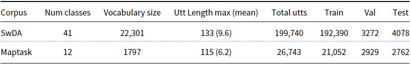
We use two corpora used throughout our experiments, the Switchboard Dialogue Act Corpus (SwDA) and the Maptask corpus. These corpora were selected primarily due to several contrasting features between them, which allows for some interesting comparisons between two quite different datasets. Firstly, SwDA contains many more utterances and has a larger vocabulary than Maptask. Secondly, the conversations within SwDA can also be considered open-domain, or non-task-oriented, while Maptask is task-oriented, and therefore the type of language used, and problem domain, is contrasted between the two. Finally, both corpora have been studied previously which provides performance baselines for comparison. The following provides an overview of each corpus, such as DA label categories, selection of training and test data, and a description of some corpus-specific pre-processing steps that were performed.Footnote b Table 1 summarises the number of DA labels, vocabulary size, utterance length, number of utterances in the training, test, and validation splits for the two corpora.
Overview of the SwDA and Maptask corpora used throughout this study
3.1.1 Switchboard
The Switchboard corpus (Godfrey et al. Reference Godfrey, Holliman and McDaniel1992) consists of telephone conversations between two participants who did not know each other and were assigned one of 70 topics to discuss. Jurafsky et al. (Reference Jurafsky, Shriberg and Biasca1997) later annotated a subset of the Switchboard corpus, using the Discourse Annotation and Markup System of Labelling (DAMSL) to form the SwDA. The corpus contains 1,155 conversations, comprising 205,000 utterances and 44 unique DA labels. During pre-processing, in some cases, it makes sense to remove or collapse several of the DA label categories. We remove all utterances marked as Non-verbal, for example, [laughter] or [throat-clearing], as these do not contain any relevant lexical information (Ribeiro et al. Reference Ribeiro, Ribeiro and De Matos2019; Stolcke et al. Reference Stolcke, Ries, Coccaro, Shriberg, Bates, Jurafsky, Taylor, Martin, Van Ess-Dykema and Meteer2000). The Abandoned and Uninterpretable labels are also merged, since these both represent disruptions to the conversation flow and consist of incomplete or fragmented utterances (Kalchbrenner and Blunsom Reference Kalchbrenner and Blunsom2013; Ribeiro et al. Reference Ribeiro, Ribeiro and De Matos2019). Some utterances are also marked as Interrupted, indicating that the utterance was interrupted but continued later in the conversation. All interrupted utterances are concatenated with their finishing segment and assigned its corresponding DA label, effectively creating full uninterrupted utterances (Webb and Hepple Reference Webb and Hepple2005; Ribeiro et al. Reference Ribeiro, Ribeiro and De Matos2019). The resulting set therefore contains a total of 41 DA labels, with the removal of non-verbal labels reducing the number of utterances by ${\sim}2\%$
. Finally, all disfluency and other annotation symbols are removed from the text.
${\sim}2\%$
. Finally, all disfluency and other annotation symbols are removed from the text.
The 1155 conversations are split into 1115 for the training set and 19 for the test set, as suggested by Stolcke et al. (Reference Stolcke, Ries, Coccaro, Shriberg, Bates, Jurafsky, Taylor, Martin, Van Ess-Dykema and Meteer2000) and widely used throughout the literature (Kalchbrenner and Blunsom Reference Kalchbrenner and Blunsom2013; Cerisara et al. Reference Cerisara, KrÁl and Lenc2017; Papalampidi et al. Reference Papalampidi, Iosif and Potamianos2017). The remaining 21 conversations are used as the validation set. It should be noted that this training and test split results in a large imbalance between two of the most common labels within the corpus, Statement-non-opinion (sd) and Statement-opinion (sv). However, to enable comparison with much of the previous work that uses this corpus, we retain this imbalanced split.
3.1.2 Maptask
The HCRC Maptask corpus (Thompson et al. Reference Thompson, Anderson, Bard, Doherty-Sneddon, Newlands and Sotillo1991) contains 128 conversations in a task-oriented cooperative problem-solving domain. Each conversation involves two participants who were given a map, one with a route and one without. The task was for the participant without the route to draw one based on discussion with the participant with the route. The transcribed utterances were annotated with 13 DA labels. However, this is reduced to 12 DA labels by removing utterances tagged with Uncodable, as these are not part of the Maptask coding scheme. As with the SwDA corpus all disfluency symbols are removed, including incomplete words, for example ‘th–‘. However, unlike the SwDA corpus, Maptask contains no punctuation, aside from a few exceptions, for example, ‘sort of ‘s’ shape’ to describe the shapes on the map. It also contains no capital letters, and we therefore do not include the Maptask corpus in the letter case and punctuation experiments.
The authors do not define any training and test data split for the Maptask corpus; we randomly split the 128 dialogues into 3 parts. The training set comprises 80% of the dialogues (102), and the test and validation sets 10% each (13), which is similar to proportions used in previous studies (Tran et al. Reference Tran, Haffari and Zukerman2017a; Tran et al. Reference Tran, Zukerman and Haffari2017b).
3.2 Models
The following section outlines the selection of sentence encoder models used throughout the experiments.Footnote c These can be separated into two categories: those trained in a fully supervised fashion and those that use a pre-trained language model to generate utterance representations. In both cases, the default classification model (component 6 described in Section 2) consists of a two-layer FFNN where the number of nodes in the final layer is equal to the number of labels in the training corpus. The final layer uses softmax activation to calculate the probability distribution over all possible labels and we use categorical cross entropy for the loss function. In the following, model hyperparameters, such as number of filters, kernel size, recurrent units, pool size and type (max or average), were all selected based on results of a Bayes search algorithm exploring a maximum of 100 parameter combinations, with each run consisting of five epochs. However, in cases where we use existing published models (i.e. excluding convolutional neural network (CNN), LSTM and gated recurrent unit (GRU)), we kept all parameters consistent with those reported in the original publications where possible.Footnote d
3.2.1 Supervised models
For the input sequence representation (letter case, punctuation, vocabulary size and sequence length) and word embeddings experiments, we use a selection of six models based on convolutional and recurrent architectures. The first layer of each model is an embedding layer and the final layer performs dimensionality reduction; either a pooling operation over the entire output sequence or outputs are simply flattened to a single-dimensional sequence representation. Thus, each of the following models encompass the embedding (2), encoder model (3) and dimensionality reduction (5) components, as described in Section 2.
CNN. The CNN is intended as a simple baseline for convolutional architectures. It consists of two convolution layers with a max pooling operation after each. We use 64 filters with a kernel size of 5 for each layer and a pool size of 8.
TextCNN. An implementation of the CNN for text classification proposed by Kim (Reference Kim2014). It is comprised of five parallel convolution layers with a max pooling operation after each. Convolutional layers use the same number of filters, 128, but with different kernel sizes in the range [1, 5]. The use of different kernel sizes is intended to capture the relationships between words at different positions within the input sentence. For dimensionality reduction, the output of each pooling operation is concatenated before flattening into a single sequence vector.
DCNN. The dynamic convolutional neural network implements the model proposed by Kalchbrenner et al. (Reference Kalchbrenner, Grefenstette and Blunsom2014). The DCNN uses a sequence of 3 convolutional layers, each with 64 filters, the first layer uses a kernel size of 7 and the following layers a kernel size of 5. In contrast to the previous convolutional models, the DCNN uses a dynamic K-max pooling operation after each convolution, which aims to capture a variable (per-layer) number of the most relevant features. Finally, dimensionality reduction is simply the flattened output of the last K-max pooling layer.
LSTM and GRU. The LSTM (Hochreiter and Schmidhuber Reference Hochreiter and Schmidhuber1997) and GRU (Cho et al. Reference Cho, Van MerriËnboer, Gulcehre, Bahdanau, Bougares, Schwenk and Bengio2014b) are simple baselines for recurrent architectures. Both models follow the standard implementation and consist of one LSTM, or GRU, layer with 256 hidden units. We take the output at each timestep and apply average (LSTM), or max (GRU) pooling for dimensionality reduction.
RCNN. The RCNN is effectively a ‘hybrid’ of recurrent and convolutional paradigms. Our implementation is based on the model proposed by Lai et al. (Reference Lai, Xu, Liu and Zhao2015) and has previously been applied to DA classification by Ribeiro et al. (Reference Ribeiro, Ribeiro and De Matos2019). The RCNN consists of two recurrent layers, each with a dimensionality of 256. One processes the sequence forwards and the other in reverse. The output of these two layers is then concatenated with the original input embedding matrix, in the format forwards-embeddings-backwards. This concatenation ‘sandwich’ is then passed as input to a convolutional layer with 64 filters and a kernel size of 1. Finally, a max pooling operation is performed for dimensionality reduction.
3.2.2 Supervised model variants
Bi-directional and Multi-layer Recurrent Models. In addition to our baseline recurrent models (LSTM and GRU), we also test their bi-directional and multi-layer variants, both of which have previously been explored within DA classification studies (Kumar et al. Reference Kumar, Agarwal, Dasgupta, Joshi and Kumar2017; Bothe et al. Reference Bothe, Magg, Weber and Wermter2018a; Chen et al. Reference Chen, Yang, Zhao, Cai and He2018; Ribeiro et al. Reference Ribeiro, Ribeiro and De Matos2019). The bi-directional models (Bi-LSTM and Bi-GRU) process the input sequence in the forwards and then backwards directions. Each pass generates a 256-dimensional vector (equivalent to the number of hidden units) per timestep, which are then concatenated to form a single 512-dimensional vector. As with the baseline recurrent models, we take the output at each timestep and apply max pooling for dimensionality reduction. The multi-layer models (Deep-LSTM and Deep-GRU) simply stack multiple recurrent layers on top of each other, with the output for a given layer, at each timestep, becoming the input for the following layer. We use the same number of hidden units and apply the same max pooling operation as the other recurrent models.Footnote e
Attentional Models. Throughout the DA classification literature, numerous studies have explored the use of different attention mechanisms (Shen and Lee Reference Shen and Lee2016; Ortega and Vu Reference Ortega and Vu2017; Tran et al. Reference Tran, Haffari and Zukerman2017a; Bothe et al. Reference Bothe, Magg, Weber and Wermter2018a; Chen et al. Reference Chen, Yang, Zhao, Cai and He2018). Though different attention mechanisms have been applied, in various contexts, we investigate the effect of adding a simple attention mechanism to each of our supervised models. During parameter tuning, we tested both additive attention (Bahdanau et al. Reference Bahdanau, Cho and Bengio2015) and multiplicative attention (Luong et al. Reference Luong, Pham and Manning2015) and found that in all cases additive resulted in the best performance. We incorporated the attention mechanism into our models by inserting an attentional layer between the utterance encoder layer and the dimensionality reduction layer. The attention layer takes as input the encoded utterance, and its output is later concatenated with the original utterance encoding, before being passed to the classification layers.
3.2.3 Language models
In addition to the supervised models, we test a selection of 10 pre-trained language models as sentence encoders. Due to the variety of model architectures, training objectives and training data that were used to generate these language models, we omit them from the input sequence experiments. Differences in training data, for example, use of punctuation, the vocabulary, and so on, would make fair comparison between the models difficult. Further, and as previously stated, the input to these models is typically a tokenised sentence, where each token is mapped to an integer representation, and does not require the further step of mapping tokens to word embeddings. Therefore, we also do not include the language models in our word embedding experiments. Instead, we use the standard input format and model parameters, defined by the original authors. The following provides a brief overview of the 10 language models, 4 of which are based on recurrent, or feed forward, neural networks, and the remaining 6 on transformer architectures (Vaswani et al. Reference Vaswani, Shazeer, Parmar, Uszkoreit, Jones, Gomez, Kaiser and Polosukhin2017).
-
NNLM The Neural Network Language Model (Bengio et al. Reference Bengio, Ducharme, Vincent, Jauvin, Kandola, Hofmann, Poggio and Shawe-Taylor2003).
-
mLSTM Character-based multiplicative long short-term memory (mLSTM) language model proposed by Krause et al. (Reference Krause, Lu, Murray and Renals2016), and applied to DA classification by Bothe et al. (Reference Bothe, Magg, Weber and Wermter2018ab).
-
ELMo Embeddings from Language Models (Peters et al. Reference Peters, Neumann, Gardner, Clark, Lee and Zettlemoyer2018).
-
USE The Universal Sentence Encoder (Cer et al. Reference Cer, Yang, Kong, Hua, Limtiaco, John, Constant, Guajardo-Cespedes, Yuan, Tar, Sung, Strope and Kurzweil2018).
-
BERT Bidirectional Encoder Representations from Transformers (Devlin et al. Reference Devlin, Chang, Lee and Toutanova2019). We use the BERT-base version, we also tested the BERT-Large model but found it did not result in any significant improvements. This also allows us to maintain a similar number of layers and parameters as other transformer models we tested, for example, RoBERTa. We also tried fine-tuning different numbers of transformer layers and found the best results were achieved with all 12 transformer blocks.
-
RoBERTa A Robustly Optimised BERT Pretraining Approach (Liu et al. Reference Liu, Ott, Goyal, Du, Joshi, Chen, Levy, Lewis, Zettlemoyer, Stoyanov and Allen2019).
-
ConveRT Conversational Representations from Transformers (Henderson et al. Reference Henderson, Casanueva, MrkŠiĆ, Su, Tsung and VuliĆ2019).
-
XLNET (Yang et al. Reference Yang, Dai, Yang, Carbonell, Salakhutdinov and Le2019).
-
GPT-2 Generative Pretrained Transformer 2 (Radford et al. Reference Radford, Wu, Child, Luan, Amodei and Sutskever2019).
-
DialoGPT The Dialogue Generative Pre-trained Transformer (Zhang et al. Reference Zhang, Sun, Galley, Chen, Brockett, Gao, Gao, Liu and Dolan2020).
3.3 Evaluation procedure
Models were trained for 10 epochs, using mini-batches of 32 sentences. Evaluation was performed on the validation set every 500 or 100 batches for SwDA and Maptask, respectively. These values allow for several evaluations per-epoch and account for the difference in the number of utterances between the two datasets.
Typically, DA classification studies evaluate performance using the accuracy metric and so to allow comparison with previous work, we also use accuracy to evaluate our models. In order to account for the effects of random initialisation and non-deterministic nature of the learning algorithms, in the next section, results reported are the average ( $\mu$
), and standard deviation (
$\mu$
), and standard deviation ( $\sigma$
), of the accuracy obtained by training and testing the model for 10 runs. Results for the validation set are the final validation accuracy, that is, the validation accuracy achieved at the end of 10 epochs. To obtain results on the test set, we first load the model weights from the point at which validation loss was lowest during training, before applying it to the test set. Therefore, results for the test set were obtained using the model that achieved the best performance on the validation set during training.
$\sigma$
), of the accuracy obtained by training and testing the model for 10 runs. Results for the validation set are the final validation accuracy, that is, the validation accuracy achieved at the end of 10 epochs. To obtain results on the test set, we first load the model weights from the point at which validation loss was lowest during training, before applying it to the test set. Therefore, results for the test set were obtained using the model that achieved the best performance on the validation set during training.
Within much of the previous DA classification literature, results reported for different models and parameter combinations often amount to very small differences in performance, usually in the region of 1–2% accuracy or less. Yet, even where results are the average over multiple runs, it is difficult to draw firm conclusions from such small differences. Thus, in order to determine if the reported mean accuracies are indeed significant, or not, we perform additional hypothesis testing. However, it is acknowledged that applying null hypothesis significance testing (NHST) can be problematic in the context of machine learning problems (Salzberg Reference Salzberg1997; Dietterich Reference Dietterich1998; Bouckaert Reference Bouckaert2003), and that the lack of independent sampling when using the same training and test data split may lead to an increased probability of type I errors. With this in mind, the following outlines our approach to significance testing, similar to that of Fiok et al. (Reference Fiok, Karwowski, Gutierrez and Reza-Davahli2020) and based on the recommendations of DemŠar (Reference Demšar2006). For cases in which the values for only one pair of parameters are compared, we use the Wilcoxon signed-rank (WSR) test, a non-parametric alternative to a dependent t-test, that makes fewer assumptions about the distribution of the data, and for which outliers have less effect. In cases where the values for multiple pairs of parameters are compared, we use a repeated measures analysis of variance (RM ANOVA). We test distributions with the Shapiro–Wilk test for normality and conclude that in most cases the two distributions were normal, though this is considered less important when using a balanced design with an equal number of samples, as in our case. A further more important assumption is sphericity, a property similar to the homogeneity of variance in standard ANOVA. We applied Mauchly’s test of sphericity and found that in all cases this assumption was met. Where the results of an RM ANOVA reveal a significant overall effect, we perform a further Tukey’s honest significant difference (Tukey’s HSD) post hoc analysis in order to determine the factors contributing to the observed effect. Throughout the analysis, we used a significance level of $\alpha = 0.05$
and conduct power analysis to ensure
$\alpha = 0.05$
and conduct power analysis to ensure $power\geq.80$
.
$power\geq.80$
.
In addition to the NHSTs, wherever we make direct comparisons between two or more classifiers, we also employ the Bayesian signed-rank (BSR) test (Benavoli et al. Reference Benavoli, Corani, DemŠar and Zaffalon2017). The BSR test was introduced by Benavoli et al. (Reference Benavoli, Corani, DemŠar and Zaffalon2017), specifically to avoid ‘the pitfalls of black and white thinking’ that accompany NHST, by analysing the likelihood that observations are significantly different. For example, for any two classifiers, A and B, we are given $P(A>B)$
,
$P(A>B)$
, $P(A==B)$
and
$P(A==B)$
and $P(B>A)$
. Thus, we are able to make a more nuanced interpretation of results than would be possible with p-values alone. Further, it does not require the same independence, or distribution, assumptions that many NHSTs do and is therefore an entirely alternative, yet complimentary, method of evaluating the differences between two classifiers. We report a result as significant, or not, only if the BSR test and the NHST independently reach the same conclusion. In such cases, we report the p-value and the most relevant probability produced by BSR test, allowing the reader to draw conclusions about the extent of the significance of the result. By additionally calculating probabilities via the BSR, we hope to alleviate some of the concerns surrounding the potential issues of NHST discussed earlier, and in so doing, establish more confidence in our reported conclusions.
$P(B>A)$
. Thus, we are able to make a more nuanced interpretation of results than would be possible with p-values alone. Further, it does not require the same independence, or distribution, assumptions that many NHSTs do and is therefore an entirely alternative, yet complimentary, method of evaluating the differences between two classifiers. We report a result as significant, or not, only if the BSR test and the NHST independently reach the same conclusion. In such cases, we report the p-value and the most relevant probability produced by BSR test, allowing the reader to draw conclusions about the extent of the significance of the result. By additionally calculating probabilities via the BSR, we hope to alleviate some of the concerns surrounding the potential issues of NHST discussed earlier, and in so doing, establish more confidence in our reported conclusions.
4. Results and discussion
In this section, we present the results and analysis for each of our sentence encoding experiments. Section 4.1 begins with the input sequence representations, before discussing the results obtained on the selection of word embeddings in Section 4.2. Sections 4.3 and 4.4 discuss results for our supervised model variants (multi-layer, bi-directional and attention). Finally, Sections 4.5 and 4.6 report final results for the selection of supervised models and language models, respectively.
For each of the input sequence and word embedding experiments, we kept all parameters fixed at a default value and only changed the parameter relevant to the given experiment. For example, when testing different vocabulary sizes, only the parameter that determined the number of words to keep in the vocabulary during text pre-processing was changed, all other parameters (letter case, use of punctuation, maximum sequence length and word embeddings) remained fixed. By default, we lower-cased all words, kept all punctuation marks and used 50-dimensional GloVe embeddings. For the SwDA corpus, the vocabulary size was set at 10,000 words with a maximum sequence length of 128 tokens, and for the Maptask corpus the vocabulary size was 1,700 words with a maximum sequence length of 115. Additionally, for all supervised models, word embeddings were fine-tuned alongside the model during training.
These default values were chosen so as not to restrict the amount of information available to the model while testing other parameters. For example, having an arbitrarily small sequence length while testing different vocabulary sizes and vice versa. Further, these values represent the upper bound of values to be tested, and are at, or near, the maximum possible value for their respective datasets. The exception being the SwDA default vocabulary size, which is less than half that of the full vocabulary. However, as discussed in 2.1.2, the typical range used for this corpus is 10,000 to 20,000 words, and Cerisara et al. (Reference Cerisara, KrÁl and Lenc2017) achieved their best results with vocabulary sizes much less than 10,000 words. While exploring sequence lengths, and vocabulary sizes, we began with small values and gradually increased until we were satisfied that further increases would not result in further improvements.
All accuracy values reported within Sections 4.1 to 4.4 are those obtained on the validation set, and only validation accuracy was used to determine the best parameters for each model. Where we report final results for the supervised models (4.5) and language models (4.6), we show results obtained on the validation and test sets.
4.1 Input sequence representations
In the following sections, we report our findings for each of the sequence representation experiments, that is, letter case and punctuation, vocabulary size and maximum sequence lengths. Due to differences in pre-training data, vocabulary, and so on, these were only carried out with the selection of supervised models, and not the language models.
4.1.1 Letter case and punctuation
Here we present the results from both the letter case and punctuation experiments, that is, during pre-processing of the text, whether to convert all mixed-case letters to lower-case letters, and whether to keep, or remove, all punctuation marks. As mentioned in Section 3.1, the Maptask corpus does not contain any words with capital letters or punctuation marks (apart from rare non-grammatical cases), and it was therefore not included in the letter case and punctuation experiments. Results for these two parameters, obtained on the SwDA corpus, are shown in Table 2.
Validation accuracy for the letter case and punctuation experiments
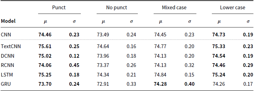
Regarding the use of punctuation, it can be seen that keeping punctuation marks results in an improvement in accuracy for all models, with a mean increase of 0.9%. Further, WSR and BSR tests comparing the punctuation and no-punctuation groups for each model confirm that this difference is statistically significant in all cases.
Similarly, with the exception of the GRU model, lower-casing all letters also improves accuracy, though to a lesser degree, with a mean increase of 0.3%. This is also statistically significant when comparing the mixed-case and lower-case groups. For the GRU, the difference between these two groups is just 0.02%, which is also not significant ( $p = 0.9$
,
$p = 0.9$
, $P(punct > no\!-\!punct) = 0.45$
), and therefore this parameter appears inconsequential for this model.
$P(punct > no\!-\!punct) = 0.45$
), and therefore this parameter appears inconsequential for this model.
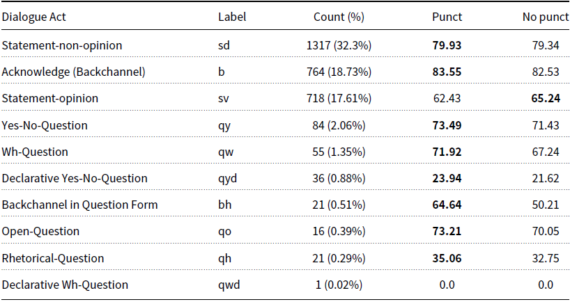
These results confirm some of the assumptions discussed in 2.1.1 and the results of Ortega et al. (Reference Ortega, Li, Vallejo, Pavel and Vu2019). Firstly, that certain punctuation marks may serve as strong indicators for the utterances DA, for example, an interrogation mark indicating a question. Table 3 shows averaged, per-label, F1 scores for the best-performing model (TextCNN), on the SwDA test set. We can see that, when punctuation is retained, F1 scores for all question-type DA labels is improved, apart from Declarative Wh-Question (qwd), which appears only once, and was not predicted. Though, collectively, the question-type labels only constitute 5.5% of all labels, and as such, this represents a minimal overall improvement. For the three most common DA labels, Statement-non-opinion (sd), Acknowledge/backchannel (b), and Statement-opinion (sv), which collectively make up 68.64% of all DA labels, the F1 score differs by $+0.59\%$
,
$+0.59\%$
, $+1.02\%$
and
$+1.02\%$
and $-2.81\%,$
respectively. This pattern is also repeated for most of the remaining labels, where small improvements are mitigated by negative changes elsewhere, resulting in the small overall accuracy increase that we have observed. This indicates that (i) punctuation marks are beneficial in more circumstances than simply a question-type DA and interrogation mark relationship, and (ii) including punctuation can also reduce accuracy for specific label types. Secondly, that lower-casing words reduces unnecessary repetition in the vocabulary, which in turn may improve learned associations between word occurrence and DA label.
$-2.81\%,$
respectively. This pattern is also repeated for most of the remaining labels, where small improvements are mitigated by negative changes elsewhere, resulting in the small overall accuracy increase that we have observed. This indicates that (i) punctuation marks are beneficial in more circumstances than simply a question-type DA and interrogation mark relationship, and (ii) including punctuation can also reduce accuracy for specific label types. Secondly, that lower-casing words reduces unnecessary repetition in the vocabulary, which in turn may improve learned associations between word occurrence and DA label.
TextCNN averaged F1 scores for the three most frequent labels (sd, b and sv), and all question-type labels (Tag-Question does not appear), in the SwDA test set.
4.1.2 Vocabulary size
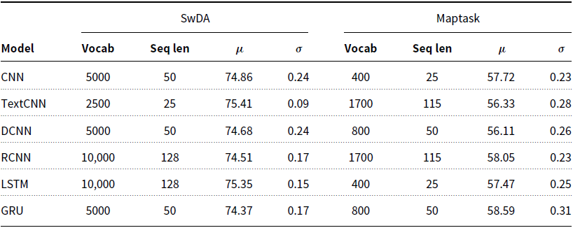
For each of the vocabulary size experiments, only the most frequently occurring words, up to the current vocabulary size, were kept within the text. Less frequent words were considered OOV and replaced with the <unk> token. We test 16 different values in the range [500, 8000] with increments of 500, and [100, 1600] with increments of 100, for SwDA and Maptask, respectively. As shown in Table 4, with the exception of the GRU applied to the SwDA, the best performance was consistently achieved using a smaller vocabulary than the largest value tested.
Vocabulary size which produced the best validation accuracy for each model on the SwDA and Maptask data
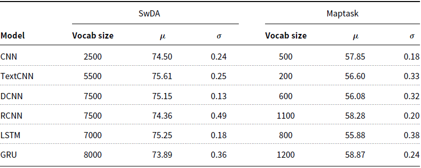
Figure 2 displays Maptask results for the full range of vocabulary sizes and models. Vertical lines indicate the average frequency of word occurrence for a given range, for example, the 200–300 most frequent words appear ${\sim}71$
times within the Maptask training data. For both SwDA and Maptask, increasing vocabulary sizes steadily improves accuracy up to
${\sim}71$
times within the Maptask training data. For both SwDA and Maptask, increasing vocabulary sizes steadily improves accuracy up to ${\sim}5k$
, or
${\sim}5k$
, or ${\sim}500$
, words respectively, beyond which further increases yield little to no improvement.
${\sim}500$
, words respectively, beyond which further increases yield little to no improvement.
Maptask validation accuracy for all supervised models with different vocabulary sizes. Vertical lines are the mean word occurrence, per-vocabulary range (up to 100 words the mean frequency = 1268, and for 100 to 200 words the mean frequency = 162).
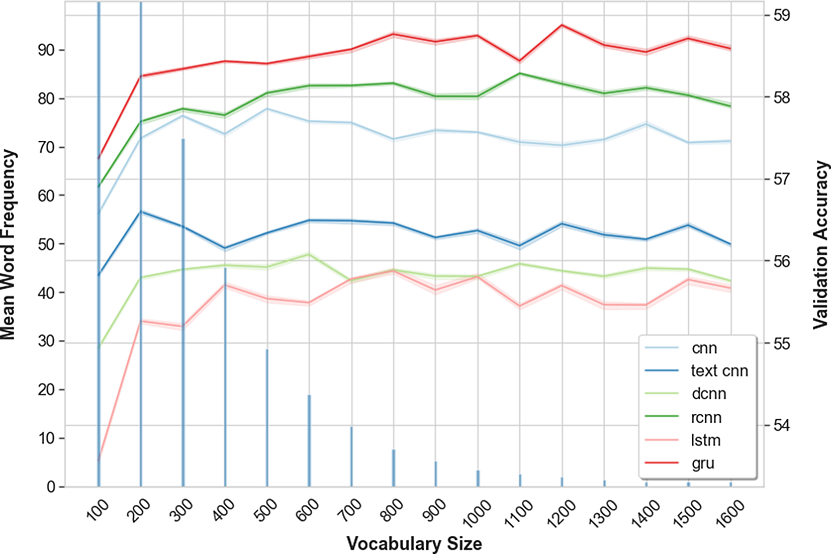
This observation noris supported by RM ANOVA followed by Tukey’s HSD post hoc analysis comparing all vocabulary size combinations, which shows that, once a threshold is reached further increase of vocabulary size does not result in a statistically significant difference in performance. For Maptask, the threshold is 400 words for all models, and for SwDA 2.5k words; except for the DCNN, where the threshold is higher, at 4k words. If we explore these thresholds in terms of frequency of word occurrences, the most frequent 2.5k and 400 words account for 95.9% and 94.7% of all words in the respective SwDA and Maptask training data. The remaining less-frequent words appear at most 22.5 or 28.3 times, within the training data, typically much less.
These results suggest that words which appear below a certain frequency within the data do not contribute to overall performance, and that word frequency is correlated with the observed performance thresholds. Either because of their sparsity within the data, or because they are not meaningfully related to any DA. On the SwDA data, the 2.5k threshold appears to coincide with the optimal 1–2k word vocabulary reported by Cerisara et al. (Reference Cerisara, KrÁl and Lenc2017). Though, apart from the CNN, we did not observe any degradation in performance from increasing vocabulary size further. Certainly, it does not appear that using large vocabularies, typically 10k or 20k words for SwDA (Ji et al. Reference Ji, Haffari and Eisenstein2016; Lee and Dernoncourt Reference Lee and Dernoncourt2016; Kumar et al. Reference Kumar, Agarwal, Dasgupta, Joshi and Kumar2017; Chen et al. Reference Chen, Yang, Zhao, Cai and He2018; Li et al. Reference Li, Lin, Collinson, Li and Chen2018), is necessary or beneficial for the DA classification task. While larger vocabularies do not create significant additional storage or computational requirements, it may be more efficient to remove very infrequently occurring words. Thus, removing a large number of words from the vocabulary which do not contribute to model performance.
4.1.3 Sequence length
To explore the effect of varying the input sequence lengths, all utterances were truncated, or padded, to a fixed number of word tokens before training. Sequences are padded with a <pad> token up to the current maximum sequence length. For both SwDA and Maptask, we test values in the range [5, 50], in increments of 5. Table 5 shows the sequence length which produced the best performance for each model. Notably, in all cases, the best validation accuracy was obtained using a sequence length that is shorter than the largest value tested, which in turn is less than half of the longest utterances in both corpora 133 and 115 words for SwDA and Maptask, respectively.
Input sequence length which produced the best validation accuracy for each model on the SwDA and Maptask data
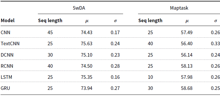
Figure 3 shows SwDA results for the full range of sequence lengths and models. Vertical lines indicate the cumulative sum of utterances, up to a given length, within the training data. It can be observed that, increasing the number of tokens steadily improves performance up to a point, beyond which we see no further improvement. On both SwDA and Maptask performance levels off at sequence lengths of ${\sim}25$
tokens.
${\sim}25$
tokens.
SwDA validation accuracy for all supervised models with different sequence lengths. Vertical lines are the cumulative sum of utterances up to a given length.
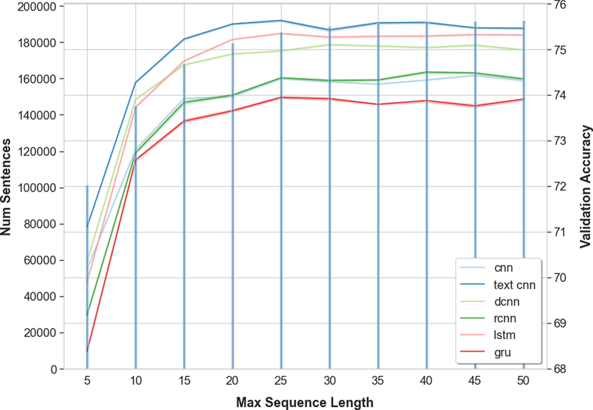
Again, these observations are supported by RM ANOVA followed by Tukey’s HSD post hoc analysis comparing all sequence length combinations, which shows that for SwDA there is no significant difference in performance for sequence lengths greater than 25 tokens, and for Maptask the threshold is 15 tokens. Examining these thresholds in terms of the frequency of utterances within the training data, 96.5% of all utterances in SwDA are <=25 words, while for Maptask 92.6% are <=15 words. This is also clearly reflected in the cumulative sum of utterance lengths as shown in Figure 3. The values closely match the shape of the accuracy curves, steadily increasing before starting to level off at the 25 or 15 token thresholds.
Our results, and the stated thresholds, for both datasets strongly support the work of Cerisara et al. (Reference Cerisara, KrÁl and Lenc2017) who found that 15–20 tokens were optimal on the SwDA data. Wan et al. (Reference Wan, Yan, Gao, Zhao, Wu and Yu2018) also reported their best result was achieved using sequence lengths of 40, which coincides with the sequence lengths that produced the best (though not statistically significant) results for some of our models. Additionally, our thresholds for both datasets and the results reported by Cerisara et al. (Reference Cerisara, KrÁl and Lenc2017) can be considered in terms of the average number of words in an English sentence. According to Cutts (Reference Cutts2013) and Dubay (Reference Dubay2004), the average number of words is 15–20 per sentence. While Deveci (Reference Deveci2019), in a survey of research articles, found the average to be 24.2 words. Thus, it should perhaps not be surprising to find that a significant proportion of utterances in our datasets are of similar or smaller, lengths.
Certainly, it seems that, similar to word occurrences, utterances above a certain length appear so infrequently that they do not contribute to overall performance. For example, in the SwDA training data, the number of utterances longer than 50 tokens is 342 (0.18%), and for Maptask it is just 11 (0.05%). Therefore, padding sequences up to the maximum utterance length does not produce any benefit, and in some cases, it may actually reduce performance (Cho et al. Reference Cho, van Merrienboer, Bahdanau and Bengio2014a). Additionally, padding sequences result in a significant increase in storage and computational effort. Instead, appropriate values should be chosen based on the distribution of utterance lengths within the data, and where possible, padding mini-batches according to the longest utterance within the batch.
4.1.4 Input sequences comparison
The vocabulary size and sequence length experiments were conducted while keeping all other parameters fixed at their default values. This leads to the possibility that using both smaller vocabularies and shorter sequence lengths, in combination, may result in too much information loss and harm performance. To explore this hypothesis, we conducted further experiments with three combinations of ‘small’, ’medium’ and ‘large’ vocabulary sizes and sequence lengths. For SwDA, we used vocabularies of 2.5k, 5k and 10k words, and for Maptask 400, 800 and 1.7k words. Each of these was combined with a respective sequence length of 25, 50 and 128 (SwDA), or 115 (Maptask). We can see from Table 6 that in most cases models achieved higher accuracy with small vocabularies and sequence lengths. RM ANOVA followed by Tukey’s HSD post hoc analysis reveals that, for the SwDA corpus, there is no significant difference between the groups for any model. Indeed, for the two models which achieved higher accuracy with the large group, RCNN and LSTM, the difference between the small and large groups mean accuracies is just 0.26% and 0.21%, respectively. For Maptask, analysis shows only three models with statistically significant results, CNN, DCNN and LSTM, each of which obtain higher accuracy with the small or medium group. Again, for the two models which favoured the large group, TextCNN and RCNN, the difference between the small and large groups mean accuracies is 0.09% and 0.25%, respectively. Thus, we can conclude that reducing both vocabulary size and sequence length does not negatively impact performance. In fact, the only cases where changing a combination of these parameters made a statistical difference is for those models which favoured smaller vocabularies and sequence lengths.
Vocabulary size and sequence length group which produced the best validation accuracy for each model on the SwDA and Maptask data
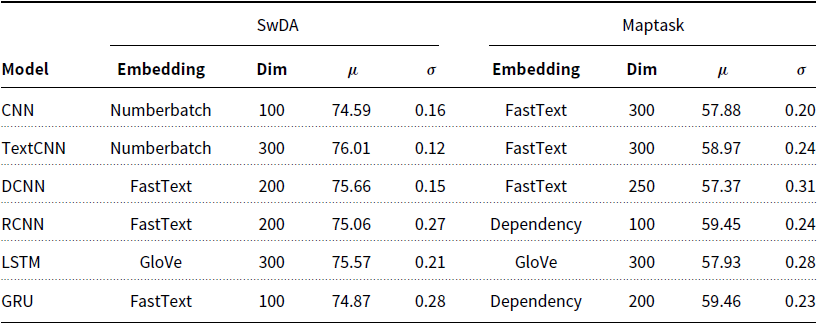
4.2 Word embeddings
Throughout our word embeddings experiments, we test five different pre-trained word embeddings; Word2Vec (Mikolov et al. Reference Mikolov, Yih and Zweig2013), trained on 100 billion words of Google News data, GloVe (Pennington et al. Reference Pennington, Socher and Manning2014), trained on 840 billion tokens of the Common Crawl dataset, FastText (Joulin et al. Reference Joulin, Grave, Bojanowski and Mikolov2017) and Dependency (Levy and Goldberg Reference Levy and Goldberg2014), which were both trained on Wikipedia data and Numberbatch (Speer et al. Reference Speer, Chin and Havasi2016), which combines data from ConceptNet, word2vec, GloVe and OpenSubtitles. Each of these is tested at five different dimensions in the range [100, 300], at increments of 50. Table 7 shows the combination of embedding type and dimension which produced the best accuracy for each model. It can be seen that there is no clearly optimal embedding type and dimension combination. Instead, it seems to be dependent on a particular task, or model, in most cases. Though, FastText does more consistently – in 50% of cases – improve performance. It is also worth noting that Word2Vec frequently resulted in poorer accuracy and therefore does not appear in Table 7 at all.
Embedding type and dimension which produced the best validation accuracy for each model on the SwDA and Maptask data
We analyse these results further by conducting a two-way RM ANOVA comparing all embedding type and dimension combinations. Across all models, and both datasets, we see no statistically significant difference between different embedding type and dimension groups. However, with the exception of the RCNN applied to the SwDA data ( $p = 0.054$
), in all cases we observe a statistically significant difference when comparing only the embedding types. To illustrate this observation, Figure 4 shows the results obtained on the SwDA data with the DCNN model. We can see that FastText and GloVe resulted in a clear improvement in performance over the remaining embedding types, and this is also true for the DCNN and LSTM applied to the Maptask data. Interestingly, the optimal embedding type and dimension for these two models is consistent across the two datasets, FastText 200–250 for the DCNN and GloVe 300 for the LSTM. For the remaining four models this is not the case, and it seems the selection of embedding type and dimension has a negligible impact on the final accuracy. As we observed in Section 2.2, in most cases the differences between embedding type and dimension is very small, and in our experiments, not statistically significant. However, for some models determining an optimal embedding type is more impactful than simply testing different dimensionalities of a single arbitrarily chosen embedding type. Additionally, Word2vec consistently underperformed on all models, and both datasets, which suggests it is not suitable for this task, a conclusion that was also reached by Cerisara et al. (Reference Cerisara, KrÁl and Lenc2017). Instead, we suggest using FastText or GloVe in the first instance as these are the only two embeddings that resulted in a significant performance increase in our experiments.
$p = 0.054$
), in all cases we observe a statistically significant difference when comparing only the embedding types. To illustrate this observation, Figure 4 shows the results obtained on the SwDA data with the DCNN model. We can see that FastText and GloVe resulted in a clear improvement in performance over the remaining embedding types, and this is also true for the DCNN and LSTM applied to the Maptask data. Interestingly, the optimal embedding type and dimension for these two models is consistent across the two datasets, FastText 200–250 for the DCNN and GloVe 300 for the LSTM. For the remaining four models this is not the case, and it seems the selection of embedding type and dimension has a negligible impact on the final accuracy. As we observed in Section 2.2, in most cases the differences between embedding type and dimension is very small, and in our experiments, not statistically significant. However, for some models determining an optimal embedding type is more impactful than simply testing different dimensionalities of a single arbitrarily chosen embedding type. Additionally, Word2vec consistently underperformed on all models, and both datasets, which suggests it is not suitable for this task, a conclusion that was also reached by Cerisara et al. (Reference Cerisara, KrÁl and Lenc2017). Instead, we suggest using FastText or GloVe in the first instance as these are the only two embeddings that resulted in a significant performance increase in our experiments.
The DCNN model’s SwDA validation accuracies for all embedding type and dimension combinations.
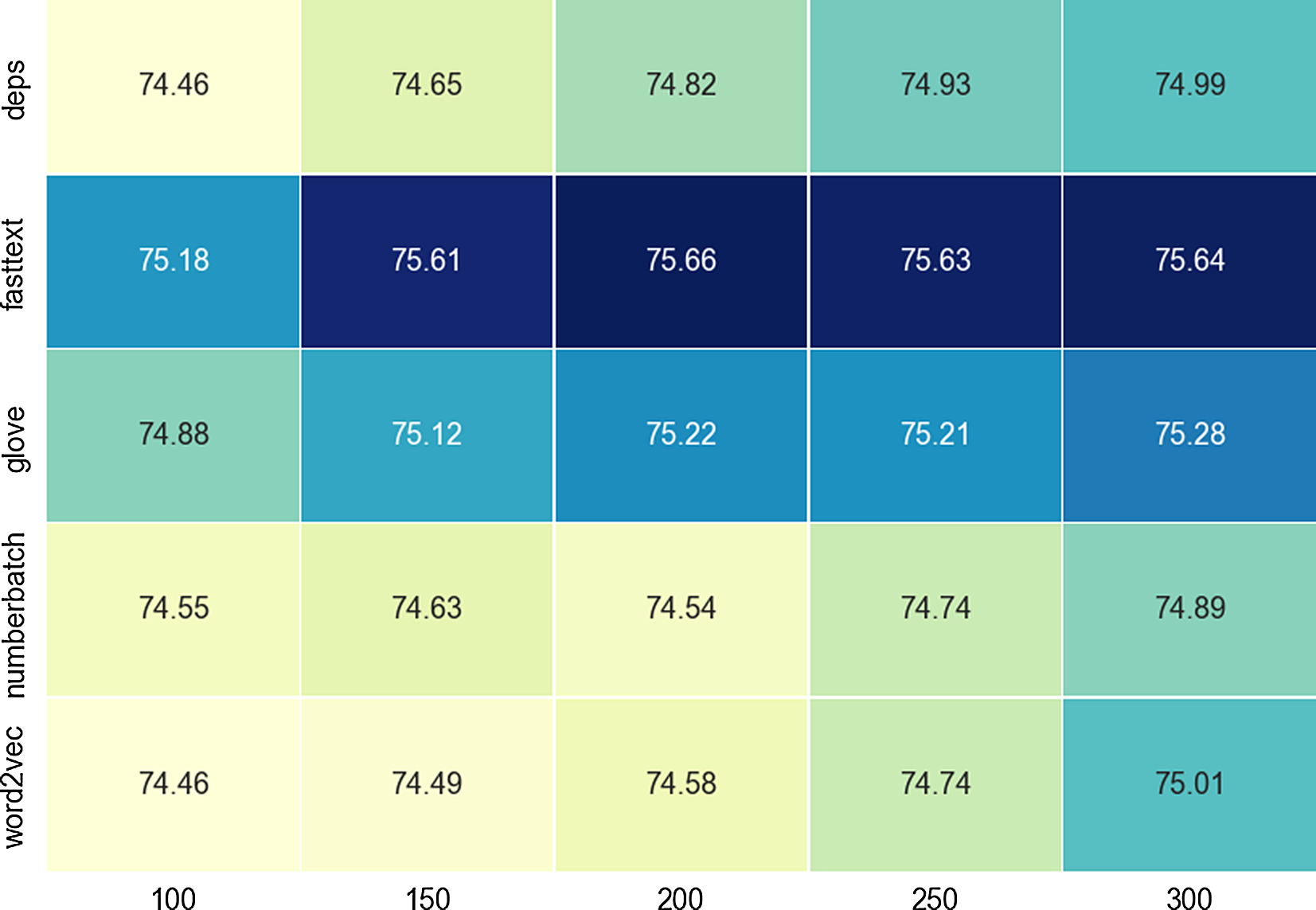
4.3 Multi-layer and Bi-directional models
For both of our recurrent models, we also experiment with increasing the number of ‘stacked’ layers and bi-directional versions, as described in Section 3.2.2. Table 8 shows our results for 1, 2 and 3-layer LSTM and GRU models on both corpora. Starting with the LSTM models, we can see that for the SwDA data the single-layer LSTM outperforms the 2- and 3-layer variants, and this is statistically significant in both cases ( $p <.001$
,
$p <.001$
, $P(\mathit{1\hbox{-} lyr} > \mathit{2/3\hbox{-} lyr}) > 0.99$
). On Maptask the 2-layer LSTM yields a small, but non-significant improvement (
$P(\mathit{1\hbox{-} lyr} > \mathit{2/3\hbox{-} lyr}) > 0.99$
). On Maptask the 2-layer LSTM yields a small, but non-significant improvement ( $p = 0.13$
,
$p = 0.13$
, $P(\mathit{1\hbox{-} lyr} > \mathit{2\hbox{-} lyr}) > 0.009$
). For the GRU models the results are inverted, with the 2-layer and 1-layer GRU resulting in better performance on SwDA and Maptask, respectively. However, in both cases, the differences between the GRU models is statistically significant (
$P(\mathit{1\hbox{-} lyr} > \mathit{2\hbox{-} lyr}) > 0.009$
). For the GRU models the results are inverted, with the 2-layer and 1-layer GRU resulting in better performance on SwDA and Maptask, respectively. However, in both cases, the differences between the GRU models is statistically significant ( $p <.003$
,
$p <.003$
, $P(\mathit{2\hbox{-} lyr} > \mathit{1\hbox{-} lyr}) = 1$
, and
$P(\mathit{2\hbox{-} lyr} > \mathit{1\hbox{-} lyr}) = 1$
, and $P(\mathit{1\hbox{-} lyr} > \mathit{2\hbox{-} lyr}) > 0.99$
). Our results for the LSTM models support those reported by Kumar et al. (Reference Kumar, Agarwal, Dasgupta, Joshi and Kumar2017) and others (Papalampidi et al. Reference Papalampidi, Iosif and Potamianos2017; Ribeiro et al. Reference Ribeiro, Ribeiro and De Matos2019), who also found that increasing the number of layers did not lead to an improvement in performance.
$P(\mathit{1\hbox{-} lyr} > \mathit{2\hbox{-} lyr}) > 0.99$
). Our results for the LSTM models support those reported by Kumar et al. (Reference Kumar, Agarwal, Dasgupta, Joshi and Kumar2017) and others (Papalampidi et al. Reference Papalampidi, Iosif and Potamianos2017; Ribeiro et al. Reference Ribeiro, Ribeiro and De Matos2019), who also found that increasing the number of layers did not lead to an improvement in performance.
Validation accuracy for 1, 2 and 3-layer recurrent models on the SwDA and Maptask data
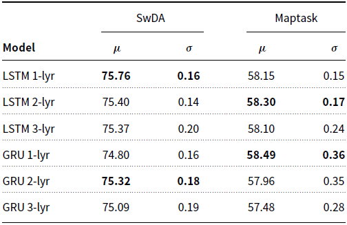
Regarding the difference we observed between the LSTM and GRU models, we speculate that this is likely due to the difference in the number of parameters between them. The single-layer LSTM has ${\sim}2.7$
million parameters, while the GRU has
${\sim}2.7$
million parameters, while the GRU has ${\sim}1.1$
million. Thus, the GRU benefitted more from an increased number of parameters when applied to the larger SwDA dataset, while the same factor may have led to overfitting on the smaller Maptask data.
${\sim}1.1$
million. Thus, the GRU benefitted more from an increased number of parameters when applied to the larger SwDA dataset, while the same factor may have led to overfitting on the smaller Maptask data.
When comparing the Bi-LSTM and Bi-GRU to their unidirectional equivalents, the only case where we observed an improvement is with the Bi-GRU applied to Maptask. However, it resulted in small increase of only 0.02% accuracy, which is unsurprisingly, not significant ( $p = 0.76$
,
$p = 0.76$
, $P(\mathit{Bi- GRU} > GRU) = 0.64$
). Bi-directional models have been employed at both the context/discourse level (Kumar et al. Reference Kumar, Agarwal, Dasgupta, Joshi and Kumar2017; Chen et al. Reference Chen, Yang, Zhao, Cai and He2018), and for sentence encoding (Bothe et al. Reference Bothe, Magg, Weber and Wermter2018a; Li et al. Reference Li, Lin, Collinson, Li and Chen2018). However, for the latter task it seems bi-directionality, at least in isolation, has no benefit.
$P(\mathit{Bi- GRU} > GRU) = 0.64$
). Bi-directional models have been employed at both the context/discourse level (Kumar et al. Reference Kumar, Agarwal, Dasgupta, Joshi and Kumar2017; Chen et al. Reference Chen, Yang, Zhao, Cai and He2018), and for sentence encoding (Bothe et al. Reference Bothe, Magg, Weber and Wermter2018a; Li et al. Reference Li, Lin, Collinson, Li and Chen2018). However, for the latter task it seems bi-directionality, at least in isolation, has no benefit.
4.4 Attentional models
For each of our supervised models, we also investigate the addition of a simple attention mechanism. During parameter tuning, we found additive attention (Bahdanau et al. Reference Bahdanau, Cho and Bengio2015), resulted in the best performance. However, our experimental results indicate that only a few models show an improvement, and in most cases attention was detrimental to performance. The CNN-Attn improved on both SwDA (0.21%) and Maptask (0.45%), though this is only significant for the Maptask data ( $p = 0.006$
,
$p = 0.006$
, $P(\mathit{CNN\!-\!attn} > CNN) = 1$
). The GRU-Attn improved on SwDA by 0.19%, which was shown to be statistically significant (
$P(\mathit{CNN\!-\!attn} > CNN) = 1$
). The GRU-Attn improved on SwDA by 0.19%, which was shown to be statistically significant ( $p < 0.03$
,
$p < 0.03$
, $P(\mathit{GRU\!-\!attn} > GRU) > 0.99$
), and the TextCNN-Attn improved on Maptask by just 0.01%. As with bi-directional recurrent models, attention mechanisms are frequently combined at both the context/discourse and sentence encoding level (Shen and Lee Reference Shen and Lee2016; Tran et al. Reference Tran, Haffari and Zukerman2017a; Tran et al. Reference Tran, Zukerman and Haffari2017b; Bothe et al. Reference Bothe, Magg, Weber and Wermter2018a; Li et al. Reference Li, Lin, Collinson, Li and Chen2018). While most of these attention mechanisms are unique implementations, and therefore not directly comparable to our experiments, it does seem that the benefit of using standard attention mechanisms for sentence encoding should be accompanied by appropriate testing to establish its true impact on performance.
$P(\mathit{GRU\!-\!attn} > GRU) > 0.99$
), and the TextCNN-Attn improved on Maptask by just 0.01%. As with bi-directional recurrent models, attention mechanisms are frequently combined at both the context/discourse and sentence encoding level (Shen and Lee Reference Shen and Lee2016; Tran et al. Reference Tran, Haffari and Zukerman2017a; Tran et al. Reference Tran, Zukerman and Haffari2017b; Bothe et al. Reference Bothe, Magg, Weber and Wermter2018a; Li et al. Reference Li, Lin, Collinson, Li and Chen2018). While most of these attention mechanisms are unique implementations, and therefore not directly comparable to our experiments, it does seem that the benefit of using standard attention mechanisms for sentence encoding should be accompanied by appropriate testing to establish its true impact on performance.
4.5 Supervised models
Here we present the final test set results for all of our supervised models. Where a variant of a model improved upon its base type that is shown instead, even if the difference was not statistically significant. In each case, the model was trained and tested using the parameters (Vocabulary size, Sequence length, etc) determined by our previous experiments. Table 9 shows results for both the SwDA and Maptask data. The TextCNN performs well on both datasets, outperforming the other convolutional models. For the recurrent models, the results are a little more variable. The LSTM achieves higher test accuracy and F1 score than the GRU on the SwDA, while for Maptask the reverse is true and by a larger margin.
Test set accuracy for each of the supervised models on the SwDA and Maptask data
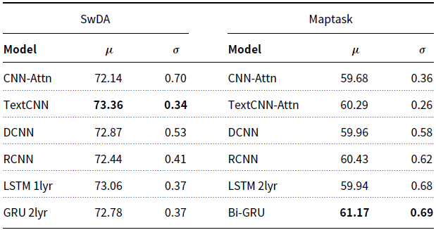
Rigorous comparison with previous work is challenging due to differences in text pre-processing and other parameters. Additionally, most recent studies do not report results for single-sentence classification, that is, DA classification without context/discourse information. Nevertheless, it seems these results are on the high end of what might be expected for single-sentence DA classification. Papalampidi et al. (Reference Papalampidi, Iosif and Potamianos2017) included salient key words as extra features in their experiment and report test set accuracy of 73.8% (though it is not clear if this result is the single best run, or an average of several), and Bothe et al. (Reference Bothe, Weber, Magg and Wermter2018b) reported 73.96% using the mLSTM language model. Yet, our TextCNN and single-layer LSTM attain similar accuracies with only pre-trained word embeddings. Our best models also outperform all of the other single-sentence results we were able to find within the literature Shen and Lee (Reference Shen and Lee2016); Cerisara et al. (Reference Cerisara, KrÁl and Lenc2017) and Lee and Dernoncourt (Reference Lee and Dernoncourt2016), who report 70.4%, 69.3% and 67%, respectively. They are also competative with, or higher than, several studies which also include context or discourse information (Kalchbrenner and Blunsom Reference Kalchbrenner and Blunsom2013; Shen and Lee Reference Shen and Lee2016; Lee and Dernoncourt Reference Lee and Dernoncourt2016; Ortega and Vu Reference Ortega and Vu2017; Cerisara et al. Reference Cerisara, KrÁl and Lenc2017), though they are far from the best contemporary approaches in that regard. However, these results do indicate that we may be at, or near, the limit of what these kinds of standard model architectures can attain for single-sentence classification. The difference between the best- and worst-performing model on the SwDA test set is just 1.22%, and for Maptask it is 1.49%. Though, small differences in accuracy are perhaps more noteworthy on the DA classification task than other classification problems. Of the studies directly comparable to ours (models that do not consider surrounding sentences, and that use the same training and test datasets), the difference between the lowest, 67% (Lee and Dernoncourt Reference Lee and Dernoncourt2016), and highest, 73.96% (Bothe et al. Reference Bothe, Weber, Magg and Wermter2018b), is just 6.96%. Further, the results of Bothe et al. (Reference Bothe, Weber, Magg and Wermter2018b) represent only a 2.96% increase over those reported by Stolcke et al. (Reference Stolcke, Ries, Coccaro, Shriberg, Bates, Jurafsky, Taylor, Martin, Van Ess-Dykema and Meteer2000), nearly two decades earlier. Thus, while some reported increases are small, parameters that produce consistent improvements, such as keeping punctuation, are meaningful for this problem. This supports the need for more sophisticated methods of sentence encoding, such as that of contextual language models.
4.6 Language models
All 10 language models were trained with the same training parameters, and default values for vocabulary size, sequence length, letter case and punctuation, as outlined in Section 4. Results for the pre-trained language models applied to the SwDa and Maptask data are shown in Table 10. Starting with the SwDA corpus, the models based on transformer architectures all resulted in an improvement in accuracy over our best-performing supervised model, TextCNN. Ranging from +0.95% with ConveRT to +2.86% for RoBERTA, and in all cases this is statistically significant ( $p < 0.001$
,
$p < 0.001$
, $P(LM > TextCNN) > 0.99$
). The remaining models show either negligible improvements or, for ELMo and NNLM, lower test set accuracy. Both BERT and RoBERTa reach test set accuracies that outperform many of the contextual models from previous studies, for example, Papalampidi et al. (Reference Papalampidi, Iosif and Potamianos2017) and Tran et al. (Reference Tran, Haffari and Zukerman2017a). They also begin to approach some of the current best contextual models, such as those reported by Bothe et al. (Reference Bothe, Magg, Weber and Wermter2018a), 77.42%, Li et al. (Reference Li, Lin, Collinson, Li and Chen2018), 78.3% and Ribeiro et al. (Reference Ribeiro, Ribeiro and De Matos2019), 79.11%.Footnote f
$P(LM > TextCNN) > 0.99$
). The remaining models show either negligible improvements or, for ELMo and NNLM, lower test set accuracy. Both BERT and RoBERTa reach test set accuracies that outperform many of the contextual models from previous studies, for example, Papalampidi et al. (Reference Papalampidi, Iosif and Potamianos2017) and Tran et al. (Reference Tran, Haffari and Zukerman2017a). They also begin to approach some of the current best contextual models, such as those reported by Bothe et al. (Reference Bothe, Magg, Weber and Wermter2018a), 77.42%, Li et al. (Reference Li, Lin, Collinson, Li and Chen2018), 78.3% and Ribeiro et al. (Reference Ribeiro, Ribeiro and De Matos2019), 79.11%.Footnote f
Validation set accuracy and test set accuracy for each of the pre-trained language models on the SwDA and Maptask data
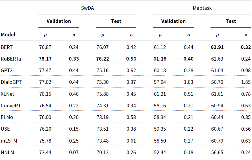
On the Maptask corpus, the language models fared much worse. Only three managed to improve upon our best supervised model, Bi-GRU, and in most cases were only marginally better than the 2nd and 3rd best. Again though, BERT and RoBERTa improve upon the supervised model by +1.74%, and +1.46%, respectively ( $p < 0.001$
,
$p < 0.001$
, $P(LM > \mathit{Bi\hbox{-}GRU}) > 0.99$
). Here comparison with previous work is more difficult as the Maptask corpus is less studied. Still, both models are comparable with the 63.3% accuracy, that is also achieved with a contextual model (Tran et al. Reference Tran, Zukerman and Haffari2017b). The relatively poor results for the Maptask data is somewhat surprising. For some of the transformer-based models, this may be due to the smaller dataset, and the comparatively larger gains in performance on the SwDA corpus would seem to support that assumption. However, it does contradict the ‘few-shot-learning’, task-specific fine-tuning, paradigm that has led to much of the success of these models (Wang et al. Reference Wang, Yao, Kwok and Ni2020). Nevertheless, both BERT and RoBERTa achieve a significant and consistent improvement on both corpora. Thus, we can conclude that – despite an increase in computational effort, training time and storage requirements – the contextual sentence representations are superior to those of supervised models and pre-trained word embeddings (Fiok et al. Reference Fiok, Karwowski, Gutierrez and Reza-Davahli2020).
$P(LM > \mathit{Bi\hbox{-}GRU}) > 0.99$
). Here comparison with previous work is more difficult as the Maptask corpus is less studied. Still, both models are comparable with the 63.3% accuracy, that is also achieved with a contextual model (Tran et al. Reference Tran, Zukerman and Haffari2017b). The relatively poor results for the Maptask data is somewhat surprising. For some of the transformer-based models, this may be due to the smaller dataset, and the comparatively larger gains in performance on the SwDA corpus would seem to support that assumption. However, it does contradict the ‘few-shot-learning’, task-specific fine-tuning, paradigm that has led to much of the success of these models (Wang et al. Reference Wang, Yao, Kwok and Ni2020). Nevertheless, both BERT and RoBERTa achieve a significant and consistent improvement on both corpora. Thus, we can conclude that – despite an increase in computational effort, training time and storage requirements – the contextual sentence representations are superior to those of supervised models and pre-trained word embeddings (Fiok et al. Reference Fiok, Karwowski, Gutierrez and Reza-Davahli2020).
5. Conclusion
This work has explored numerous factors which may affect the task of sentence encoding for the purpose of DA classification. We first considered various aspects of text pre-processing and representation, which are often overlooked or underreported within the literature, such as whether to keep or remove punctuation, selecting vocabulary size, input sequence length and word embeddings. Each of these was assessed on the SwDA and Maptask corpora, using a selection of six supervised models, that are intended to be representative of the common architectures applied to DA classification task. Finally, we also applied a selection of 10 pre-trained language models, including transformer-based contextual language models, such as BERT and XLNET, and draw comparisons between the supervised approaches. To the best of our knowledge, this is also the first time most of these comparatively new language models have been applied to the DA classification problem.
Our findings indicate that, for each of the text pre-processing parameters we investigate, selecting the right values can have a small but statistically significant effect on final classification accuracy.
Firstly, converting all words to lower case and keeping all punctuation always improve accuracy when compared to the alternative options, though lower-casing is less impactful. Interestingly, keeping punctuation appears beneficial for several of the most common DA labels within the SwDA corpus, even those that are not a type of question, where intuitively one might expect an interrogation mark to strongly correlate with a question type DA label. Unfortunately, this benefit is partially mitigated by the negative impact keeping punctuation has for several other label types.
Considering the selection of vocabulary size, we found that using smaller vocabularies was beneficial in most cases. Certainly, our results show that the number of words, for the best-performing models, was $\frac{1}{4}$
to
$\frac{1}{4}$
to $\frac{3}{4}$
of the largest vocabulary size tested, which equates to around 1/10th of the corpora’s full vocabulary. Additionally, increasing vocabulary sizes results in diminishing, or detrimental, returns in performance. For the SwDA, beyond the threshold of 2.5k words, most models showed no statistically significant improvement in accuracy, while on the Maptask data the threshold is 400 words. These values are much lower than those typically used in most DA classification studies (where such parameters are reported), for example, 10k or 20k words for SwDA (Ji et al. Reference Ji, Haffari and Eisenstein2016; Lee and Dernoncourt Reference Lee and Dernoncourt2016; Li et al. Reference Li, Lin, Collinson, Li and Chen2018; Kumar et al. Reference Kumar, Agarwal, Dasgupta, Joshi and Kumar2017; Chen et al. Reference Chen, Yang, Zhao, Cai and He2018). Instead we recommend using smaller vocabularies to prune out highly infrequent words which are unlikely to be relevant to the DA classification task and to reduce noise within the data.
$\frac{3}{4}$
of the largest vocabulary size tested, which equates to around 1/10th of the corpora’s full vocabulary. Additionally, increasing vocabulary sizes results in diminishing, or detrimental, returns in performance. For the SwDA, beyond the threshold of 2.5k words, most models showed no statistically significant improvement in accuracy, while on the Maptask data the threshold is 400 words. These values are much lower than those typically used in most DA classification studies (where such parameters are reported), for example, 10k or 20k words for SwDA (Ji et al. Reference Ji, Haffari and Eisenstein2016; Lee and Dernoncourt Reference Lee and Dernoncourt2016; Li et al. Reference Li, Lin, Collinson, Li and Chen2018; Kumar et al. Reference Kumar, Agarwal, Dasgupta, Joshi and Kumar2017; Chen et al. Reference Chen, Yang, Zhao, Cai and He2018). Instead we recommend using smaller vocabularies to prune out highly infrequent words which are unlikely to be relevant to the DA classification task and to reduce noise within the data.
Similarly, for input sequence lengths, we showed that beyond a certain threshold using longer sequences has no significant impact on classification accuracy. For SwDA, the threshold is 25 words, and for Maptask 15. These thresholds, and the optimal sequence lengths for all models, on both datasets, were shorter than the maximum sequence length we tested (50 tokens), which in turn is < 50% of the longest utterances in either corpora. Thus, we conclude that padding sequences to lengths nearer that of the longest utterances in the data is a tremendous waste of computational effort and storage. We also found that calculating the cumulative frequency of utterance lengths within the data produced a reasonable approximation of the resulting accuracy curves within our experiments. When the cumulative frequency began to level off, so too did the model’s accuracy. This technique could be used to select a viable sequence length which minimises both information loss (through truncation) and the number of unnecessary padding tokens. We leave further investigation of this observation for future work. It should also be noted that when using smaller vocabularies and sequence lengths in combination, we observed no significant difference when compared to larger valued combinations. Certainly, in most cases, including the best-performing models, higher accuracies were achieved when using a combination of smaller values.
Results for our word embedding experiments were perhaps less conclusive. Of the pre-trained embeddings we tested, none was shown to be clearly optimal across both datasets and models. Though FastText embeddings, with dimensions in the range [200, 300], did result in the highest validation accuracies in 50% of cases. It seems that the selection of embedding is highly dependent on both model and data, though the overall impact of this choice is often negligible. This is supported by our statistical analysis which showed that, when comparing all embedding type and dimension combinations, we only observed a statistically significant difference in performance when comparing different embedding types. Thus, while choice of embedding may result in a small (and likely statistically non-significant) effect on performance, the selection of embedding type tends to be more impactful than the dimension.
For each of our six supervised models, we also experimented with some architectural variations that are frequently adopted within classification studies. With the recurrent models (LSTM and GRU), we tried both bi-directionality and increasing the number of layers. In only a few cases, these resulted in a small, but not significant, improvement. We also tried adding an attention layer to all six models. Again, in only a few cases did this result in any accuracy improvement. Though in two cases this was shown to be statistically significant; the GRU-Attn applied to the SwDA data, and the CNN-Attn applied to Maptask. It is conceded that the effect of these architectural variations may have a greater impact with regard to contextual DA classification models, rather than the single-sentence approach explored here. However, despite how frequently bi-directional, multi-layer and attentional models are applied to DA classification (Bothe et al. Reference Bothe, Magg, Weber and Wermter2018a; Chen et al. Reference Chen, Yang, Zhao, Cai and He2018; Li et al. Reference Li, Lin, Collinson, Li and Chen2018), they are rarely accompanied by appropriate ablation studies to determine help quantify the true impact such additions have on overall performance. Test set accuracy achieved by our best-performing models (TextCNN and LSTM) on the SwDA data is in most cases much higher than, or equivalent to, results reported by previous single-sentence classification studies. We were not able to find any results for non-contextual DA classification for the Maptask corpus. However, comparing our results for the supervised and language models on this corpus, we suspect the same would be true here. These results were also obtained using standard model architectures, with smaller vocabularies and input sequence lengths than are typically used, and without any additional feature engineering.
Results from our language model experiments are somewhat mixed. None of the non-transformer-based models was able to achieve a statistically significant improvement on either dataset, in many cases it was lower than our supervised models. However, on the SwDA data, each of the transformer-based contextual language models show a significant improvement over the supervised approach. Notably, both BERT and RoBERTa achieve test set accuracies of 76.07% and 76.22%, an increase of +2.71% and +2.86%, respectively, when compared to our best-performing supervised model, TextCNN. These values surpass the reported accuracies for much of the previous DA classification approaches which also consider discourse/contextual features. However, on the Maptask data, the transformer-based models fared less well. Only BERT and RoBERTa obtained a significant improvement in test set accuracy over the best-performing supervised model, Bi-GRU. Here, we see a less dramatic improvement of 1.74% and 1.46%, respectively. Thus, we can conclude that the contextual sentence representations produced by BERT-type models are a significant improvement over those produced by our other fine-tuned language models or supervised models.
Throughout this work, we have shown that the text pre-processing parameters we investigated should not be arbitrarily chosen, because they can produce a notable effect on model performance. Particularly, instead of using large vocabularies and sequence lengths, where it becomes computationally wasteful, it is often beneficial to use smaller values. Additionally, the optimal values we found for these two parameters are much smaller than those typically used. We hope this work can be used as a point of reference for future research when considering these aspects, and that each of them might be worthy of further investigation. Regarding the selection of models, we found that performance was often inconsistent when applying the same, or similar, architecture to different datasets. Most notably, the use of bi-directional or multi-layered recurrent architecture, or the addition of attention layers – which are so frequently applied to DA classification–often did not yield any improvement over their simpler baseline version. These inconsistencies suggest that these architectural additions should be accompanied by appropriate ablation experiments to determine their true impact on performance. And further, applying a single model, or small variations thereof, to a single dataset is not enough to draw firm conclusions on its generalisable performance. This is similarly true for the selection of language models we tested. Where, even amongst the transformer-based models, on the smaller, sparser, Maptask data some models failed to improve upon our best-performing supervised model. However, on both datasets, BERT and RoBERTa represent a significant improvement in sentence encoding for DA classification and are therefore the current best choice for applying to this task.
A. Model parameters
Parameters for the (base) supervised and language models
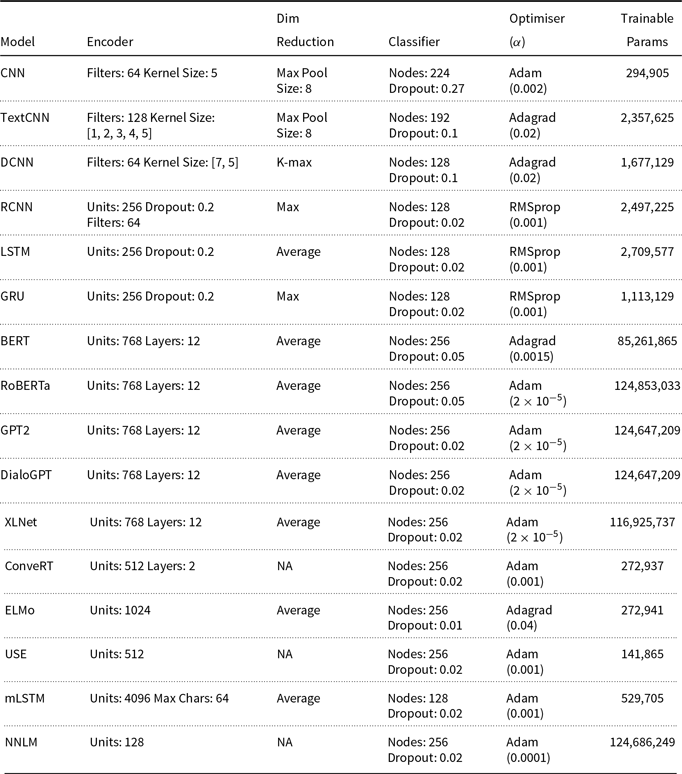


 Open access