

Introduction
This paper will focus on the ∼60% of the mineral kingdom that is dielectric, i.e. the valence electrons are bound and the crystals are insulators. For convenience, I will refer to the atoms of these minerals as cations and anions. However, these terms have no connection with previous model(s) of ionic bonding. The term ‘cation’ here refers to atoms of low electronegativity and the term ‘anion’ refers to atoms of high electronegativity, reflecting the bipartite nature of the inorganic structures which I shall consider below. In the interest of clarity, I define certain terms used in the following text:
‘Coordination number’: The number of counterions bonded to an ion.
‘Coordination polyhedron’: The arrangement of counterions around an ion.
‘Ion configuration’: A unique arrangement of ion type and coordination number.
‘Characteristic bond length’: the grand mean bond length for a cation in a particular ion configuration.
‘Characteristic coordination number’: The weighted grand mean coordination number of a cation in all its ion configurations.
There is a long history of our views on atoms, stretching from Leucippus of Miletus (or Elea) (480–420 BC), and Democritus of Abdera (460–370 BC) to the present day, a brief summary of which is given by Hawthorne (Reference Hawthorne2006). The first inductive work on the arrangement of ‘atoms’ in materials is due to Johannes Keppler (1571–1630) who proposed that snowflakes are composed of a planar close-packed arrangement of spherical ‘atoms’ of ice. The first quantitative predictions of crystal structure were made by William Barlow (1845–1934) who used a combination of symmetry relations and packing considerations to predict the correct structures for the alkali halides (Barlow, Reference Barlow1883, Reference Barlow1898). Bragg (Reference Bragg1913) initiated the experimental characterization of crystal structures at the atomic level and showed that Barlow’s predictions are correct, initiating the systematic solution of crystal structures. Treating atoms as ions, early crystallographers evolved a series of ideas to help derive atomic arrangements from diffraction data. Ions were assigned different sizes (e.g. Landé, Reference Landé1920) and Hüttig (Reference Hüttig1920) proposed that the coordination number of cations in molecular complexes is determined by radius-ratio considerations. Goldschmidt (Reference Goldschmidt1926, Reference Goldschmidt1927) was the first to use these coordination-number arguments to predict coordination numbers for a wide range of cations in crystals (Jensen, Reference Jensen2010). These ideas were collected and further developed by Pauling (Reference Pauling1929, Reference Pauling1960) who consolidated them as a set of relatively simple yet effective rules for understanding and predicting stable atomic arrangements in ‘ionic crystals’, primarily oxide-based minerals and inorganic compounds.
Pauling’s rules have formed the basis of Crystal Chemistry for nearly a century and are still taught in introductory courses in Mineralogy and Inorganic Chemistry. The first two rules are of particular significance in this regard:
(1) The radius-ratio rule: “A coordinated polyhedron of anions is formed about each cation, the cation-anion distance being determined by the radius sum and the ligancy of the cation by the radius ratio.”
The deficiencies in this rule have been discussed extensively (e.g. Michmerhuizen et al., Reference Michmerhuizen, Rose, Annankra and Vander Griend2017; George et al., Reference George, Waroquiers, Stefano, Petretto, Rignanese and Hautier2020; Gibbs et al., Reference Gibbs, Hawthorne and Brown2022; Hawthorne and Gagné, Reference Hawthorne and Gagné2024).
(2) The electrostatic valence rule: “Let z be the electric charge of a cation and v its coordination number; we then define the strength of the electrostatic bond to each coordinated anion as s = z/v, and make the postulate that in a stable ionic structure, the valence of each anion, with changed sign, is exactly or nearly equal to the sum of the strengths of the electrostatic bonds to it from the adjacent cations.”
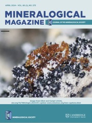
As discussed in detail by Gibbs et al. (Reference Gibbs, Hawthorne and Brown2022), there have been numerous developments stemming from the second rule, the most significant of which is Bond-Valence Theory (Brown Reference Brown, O’Keeffe and Navrotsky1981, Reference Brown2002, Reference Brown2016). A commonly used feature of Pauling’s second rule is the ‘bond-strength table’ which lists bond strengths from the cations to the anions and sums of the bond strengths incident at each ion in a crystal structure. Table 1 shows the Pauling bond-strength table for tremolite, ideally Ca2Mg5Si8O22(OH)2, which illustrates the argument that Warren (Reference Warren1930a, Reference Warren1930b) used to show that H (as OH) is an essential constituent of common amphiboles, thereby resolving a longstanding and controversial issue. Bond-strength and bond-valence tables are now used widely: (1) to check the validity of a refined crystal-structure; (2) to determine the oxidation states of constituent polyvalent ions in a crystal (e.g. Fe2+/Fe3+, Mn2+/Mn3+); and (3) to identify the charges of both simple (e.g. O2–, F–) and complex [(OH)–, (NH4)+] ions, particularly where those ions are involved in positional disorder.
Pauling bond-strength table for tremolite*

Table 1 Long description
The table lists bond-strength contributions from three magnesium positions, one calcium position, and two silicon positions to seven oxygen sites in tremolite, along with a total for each oxygen. Oxygen sites O5 and O6 have the largest totals, 2.25 each, coming from calcium plus one contribution each from the two silicon positions. O1 and O7 total 2.00; O1 combines magnesium contributions with one silicon contribution, while O7 is supplied only by silicon. O2 totals 1.92, with magnesium contributions plus calcium and one silicon contribution. O4 totals 1.58, combining magnesium, calcium, and one silicon contribution. O3 is the smallest at 1.00 and is made only from magnesium contributions. Column totals indicate each magnesium and calcium position sums to 2 overall, and each silicon position sums to 4 overall, with totals adjusted to match the stated rounding.
* Bond strengths to two decimal places, sums adjusted.
Problems with the ionic model
The chapter dealing with the bond-strength model in Pauling (Reference Pauling1960) is entitled ‘The Sizes of Ions and the Structure of Ionic Crystals’. We know that crystals contain ions; if electron density were not delocalized from each atom in the direction of the neighbouring atoms, there would be no chemical bonds to hold the atoms of a molecule or a crystal together. However, in the ‘ionic model’, the valence electrons of the more electropositive atom are totally transferred to the more electronegative atom to form completely filled shells in both atoms, with integer residual charges on both atoms (i.e. ions). This implies that each ion is spherical and that there is no electron density delocalized between the closest ions. We know that this is not correct: (1) in experimental electron-density maps, electron density is observed along what we consider as chemical bonds; and (2) quantum mechanics indicates that atomic orbitals hybridize to form molecular orbitals that contain electron density shared between bonded atoms. Such delocalized electron density has been imaged by laser picoscopy (Fig. 1) and ‘residual charge’ is left on the cations due to incomplete ionization (Table 2). We acknowledge this situation by considering that ‘ionic bonds’ are partly covalent and ‘covalent bonds’ are partly ionic, but this does not change the fact that we know that our ‘ionic model’ is physically wrong. However, it is still useful in some respects and we continue to use it.
Right: Laser picoscopy image of the valence-electron density in MgF2; Left: valence potential (blue curves) when the laser polarization vector is aligned with [110]. Modified from Lakhotia et al. (Reference Lakhotia, Kim, Zhan, Hu, Meng and Goulielmakis2020).

Figure 1 Long description
Panel A: A line graph illustrating valence potential when the laser polarization vector is aligned with [110]. The x-axis is labeled 'Distance (angstrom)' ranging from 0 to 6 and the y-axis is labeled 'Potential (arbitrary units)' ranging from minus 1.0 to 0.0. The blue curve oscillates, showing minima at approximately 1 angstrom, 3 angstrom and 5 angstrom and maxima near 2 angstrom and 4 angstrom. Above the curve, ions are labeled as 'F', 'Mg superscript 2 plus' and 'F', indicating the positions of fluoride and magnesium ions. Panel B: A heatmap representing valence-electron density in MgF. Both axes are labeled 'Distance (angstrom)' ranging from 0 to 4. The color scale above the heatmap ranges from minus 1.0 to 0.0, indicating intensity levels. The pattern is symmetric, with alternating regions of higher and lower density, forming a checkerboard-like appearance. Maxima occur at the center and corners, while minima are located between these points. The heatmap visually represents electron density distribution, highlighting periodicity and symmetry in the material structure.
Charges at atoms in M 2+2Si2O6 pyroxene structures determined by charge-density refinement of X-ray diffraction data*

Table 2 Long description
The table lists refined atomic charges for pyroxenes with three different divalent cations: magnesium, iron, and cobalt. For the magnesium-bearing structure, the M2 cation is plus 1.82, silicon is plus 2.28, and oxygen sites range from minus 1.27 to minus 1.42, with the terminal oxygen most negative. For the iron-bearing structure, the M2 cation drops to plus 1.12 while silicon stays at plus 2.28, and oxygen sites are less negative overall, from minus 0.97 to minus 1.13. For the cobalt-bearing structure, the M2 cation is plus 0.95, silicon is slightly lower at plus 2.19, and oxygen sites range from minus 1.05 to minus 1.13. Comparing columns, the M2 charge decreases from magnesium to iron to cobalt, and the oxygen charges generally become less negative over the same sequence. Within each structure, silicon remains the most positive site and oxygen remains negative, with terminal oxygen typically the most negative among the oxygen entries. Values are refinement-derived and should be interpreted as model-dependent estimates rather than exact ionic charges.
* values from Sasaki et al. (Reference Sasaki, Takeuchi, Fujino and Akimoto1982)
Bonded atoms
If two neutral atoms A and B are far apart, they each will have spherical symmetry. As they approach each other, the protons in the nucleus of atom A will exert an attractive force on the electron density of atom B and this electron density will move towards atom A, and vice versa for the electron density of atom A. This delocalized electron-density may be represented as: (1) occupying molecular orbitals; or as (2) electron density dispersed along the A–B axis between the two atoms. Both models describe the occurrence of electron density between the two atoms, and this delocalized electron density may be described pragmatically as the chemical bond that is the binding force for both molecules and crystals.
Point-charge models
An arrangement of point charges is not stable (Earnshaw, Reference Earnshaw1842). Thus Earnshaw’s theorem prevents the existence of a stable completely ionic crystal. If such an arrangement were stable, a small perturbation of a charged particle from its equilibrium position would induce a restoring force on that particle, requiring the divergence of the electric field to be negative. Such a condition contradicts Gauss’s law which requires that the divergence of an electric field is zero in free space. This issue was finally resolved only with the advent of quantum theory which proposed the currently accepted modal of the atom in which electrons occupy orbitals around the nucleus. Where atoms approach each other, the valence electrons delocalize, the spherical symmetry of the atom is broken, the local charge of each atom (ion) no longer has spherical symmetry and cannot be considered as a point charge, and Earnshaw’s theorem no longer applies.
Using graphs to represent crystal structures
A graph is defined as a non-empty set of elements, V(G), called ‘vertices’, and a non-empty set of unordered pairs of these vertices, E(G), called ‘edges’ (Wilson, Reference Wilson1979). We may draw a pictorial representation of a simple graph with four vertices and four edges as shown in Fig. 2a. The number of edges meeting at a vertex is the ‘degree’ of that vertex. Let Fig. 2b represent a (hypothetical) square molecule in which the lines represent chemical bonds between the individual atoms. The graph (Fig. 2a) retains the bond topological information of the molecule (Fig. 2b) but does not have the same metrics (i.e. distance is defined in a different way: e.g. length is the number of edges between two vertices). We may input additional information into the graph of Fig. 2a: (1) the vertices may be assigned labels to differentiate between them; (2) the vertices may be assigned colours to designate different types of vertices; (3) the edges may be assigned weights to designate different types of edges; (4) the edges may be assigned directions (to form a digraph) to represent different vector properties. The resulting graph (Fig. 2c) is a ‘labelled polychromatic weighted digraph’. The hypothetical square molecule (Fig. 2b) may have different atoms at each corner corresponding to the labels and colours of the vertices of the graph. The bonds of the square molecule correspond to the edges of the graph (that are differentiated by the vertex pair at each end of the edge), and the (bond) strength of each bond corresponds to the weight of the corresponding edge. As noted above, we are dealing with (partly ionized) atoms which link via electrostatic interaction between valence electrons of one atom and protons of the bonded atom (and vice versa). The electric field that moderates these interactions is a vector field and the chemical bonds have directions: + (positive from cation to anion) and – (negative from anion to cation); hence each bond has a direction (+ive or –ive) corresponding to the directions of the edges in a directed graph. There is a one-to-one homeomorphic mapping of the atoms of this square molecule (Fig. 2b) onto the vertex set of the graph (Fig. 2c) and of the chemical bonds of the molecule onto the edge set of the graph. The graph retains the bond topological information of the molecule but does not have the same metrics.
(a) A simple graph of four vertices of degree 2 and four edges; (b) a hypothetical square molecule M 2N2; (c) a labelled polychromatic weighted digraph.

Figure 2 Long description
The image A shows a simple graph with four vertices and four edges. Each vertex is connected to two others, forming a square shape. The vertices are unlabeled and the edges are undirected. The image B depicts a hypothetical square molecule with four vertices labeled as M superscript n plus and N superscript n minus. The vertices are connected by lines representing chemical bonds, with directions indicated by plus and minus signs. The image C illustrates a labelled polychromatic weighted digraph with four vertices numbered 1, 2, 3 and 4. The vertices are colored purple and yellow. Directed edges connect the vertices, with arrows indicating direction and weights labeled as w subscript 12, w subscript 23, w subscript 34 and w subscript 41. The edges form a square, similar to the previous images, but with directional and weighted properties.
There are many advantages of using this graphical representation of structure (e.g. Hawthorne, Reference Hawthorne1983; Day and Hawthorne, Reference Day and Hawthorne2020, Reference Day and Hawthorne2022; Day et al., Reference Day, Hawthorne and Rostami2024a, Reference Day, Rostami and Hawthorne2024b). Perhaps the major advantage is that the graph in Fig. 2c may be represented by a matrix in which each row and column of the matrix is associated with a specific coloured labelled vertex. The corresponding matrix entries (non-zero or zero) denote whether two vertices are adjacent (that is, joined by an edge) or not. This matrix is called an ‘adjacency matrix’ (Fig. 3). In a digraph, the ‘indegree’ of a vertex is the number of edges ‘incident’ at that vertex, and the ‘outdegree’ of a vertex is the number of edges ‘exident’ at that vertex. In a ‘bipartite graph’, the vertices form two disjoint (and independent) sets and every edge connects a vertex in one set to a vertex in the other set. In a ‘bipartite digraph’, all vertices in one set are exident and all vertices in the other set are incident. Equivalently, a bipartite graph is a graph that does not contain any odd-length cycle. Hence bipartite digraphs are ideal representations of crystal structures consisting of cations and anions. Figure 2c represents a molecule; how do we represent a (translationally symmetric) crystal structure? Any graph-theoretic representation of such a structure is (quasi-) infinite and infinite graphs are an unsolved problem. However, in using graphs to represent crystals, the structures are translationally symmetric as well as (quasi-) infinite. This allowed us to develop a procedure that we term ‘wrapping’ (described in detail by Day and Hawthorne, Reference Day and Hawthorne2022; Day et al., Reference Day, Hawthorne and Rostami2024a, Reference Day, Rostami and Hawthorne2024b) that allows graphical exploration of the bond topology of crystal structures.
The adjacency matrix corresponding to the labelled polychromatic weighted digraph.

Figure 3 Long description
The table has four columns labeled 1, 2, 3 and 4. Row 1: 1 -; 2 w12; 3 0; 4 w14. Row 2: 1 w21; 2 -; 3 w23; 4 0. Row 3: 1 0; 2 w32; 3 -; 4 w34. Row 4: 1 w14; 2 0; 3 w43; 4 -. Each entry represents the weight of the edge between vertices, with '-' indicating no edge.
The bond-strength model
Coulomb’s Law states that ‘the magnitude of the electrostatic force of attraction or repulsion between two point charges is directly proportional to the product of the magnitudes of charges and inversely proportional to the square of the distance between them’. Electric charge is thus a continuously differentiable function and hence is subject to a conservation law as required by Noether’s first theorem (Noether, Reference Noether1918; Quigg, Reference Quigg2013), and the global gauge invariance of the electric field results in the conservation of electric charge.
Consider the Pauling bond-strength table for a monoclinic pyroxene CaM2+Si2O6 (Table 3). The bond strengths exident from each cation are calculated as the cation charge divided by the cation coordination number. As a result, all bond strengths exident from a particular cation-site are equal. Gauss’s law requires the sum of the bond strengths exident from the cation site to be equal to the cation charge; it does not require the exident bond strengths to be equal. The result is that the bond strengths incident at the anion sites are not correct, and inspection of Table 3 shows that conservation of charge is not obeyed at the anions.
Pauling bond-strength table for C2/m pyroxenes CaM 2+Si2O6

Table 3 Long description
The table lists Pauling-style bond-strength contributions from calcium in eightfold coordination, a divalent M cation in sixfold coordination, and silicon in fourfold coordination to three oxygen sites labeled O1 to O3, plus each oxygen’s total anion bond strength. For O1, calcium contributes 0.250 and the M cation contributes 0.333, while silicon contributes 1.00, giving a total of 1.916. For O2, calcium again contributes 0.250 and the M cation contributes 0.333, with silicon at 1.00, for a lower total of 1.583. O3 shows calcium at 0.250, no listed M-cation contribution, and silicon at 1.00, producing the highest total of 2.500. Overall, the totals rank O3 highest, then O1, then O2, indicating the strongest summed bonding at O3 and the weakest at O2. A final row reports total cation counts of 2 for calcium, 2 for the M cation, and 4 for silicon; the arrow and multiplicity markers indicate repeated bonds but are not expanded into explicit calculations here.
A priori bond strengths: definition and calculation
The term ‘bond strength’ is used widely to refer to bond strengths as evaluated by Pauling (Reference Pauling1929, Reference Pauling1960). In order to distinguish between the calculation of bond strengths as done here and as done by Pauling (Reference Pauling1929, Reference Pauling1960), I use the term ‘Pauling bond-strengths’. “A priori bond-strengths are calculated from the bond topology (structure connectivity) of a structure and the charges of all the ions in that structure using all aspects of the conservation law of the electric field.” I use the term a priori to emphasize that no Euclidian metrics are used in the calculation. The method of calculating a priori bond strengths follows that of Gagné et al. (Reference Gagné, Mercier and Hawthorne2018) for bond valences.
Table 4 shows the bond-strength table for C2/m CaM 2+Si2O6 pyroxenes in which the bond strengths are represented by the variables a to h with the constraints that the sums of the bond strengths exident from the cations and the anions are equal to the magnitudes of the formal charges of the cations and the anions. There are eight variables in Table 3 and six simultaneous equations. The solution of such systems of simultaneous equations is governed by the Rouché-Capelli theorem (Shafarevich and Remizov, Reference Shafarevich and Remizov2013; page 58): “A system of linear equations with n variables has a solution if and only if the rank of its coefficient matrix A is equal to the rank of its augmented matrix [A|b]” where, for the applications described here, [b] is the column matrix involving the magnitudes of the formal charges of the ions in the structure. The system of simultaneous equations derived from Table 4 does not have a solution according to the above condition; what else can we do?
A priori bond-strength table for C2/m pyroxenes CaM 2+Si2O6

Table 4 Long description
The table summarizes a priori bond strengths for a C2 slash m pyroxene with calcium, a divalent M cation, and silicon, organized by oxygen sites and cation coordination groups. Rows list three oxygen positions, each with an anion total of 2. Columns list calcium in eightfold coordination, M2 plus in sixfold coordination, and silicon in fourfold coordination, with lettered bond-strength entries and multiplicities indicated by counts and arrows. For oxygen site 1, calcium has two downward bonds labeled a, M2 plus has four downward and two rightward bonds labeled d, and silicon has one bond labeled f. For oxygen site 2, calcium has two downward bonds labeled b, M2 plus has two downward bonds labeled e, and silicon has one bond labeled g. For oxygen site 3, calcium has four downward and two rightward bonds labeled c, M2 plus is blank, and silicon has two downward and two rightward bonds labeled h. The bottom totals indicate 2 for calcium, 2 for M2 plus, and 4 for silicon, consistent with the intended cation sums across the structure. Letter labels represent bond-strength categories rather than numeric values, so comparisons are qualitative and based on presence and multiplicity, not magnitude.
The electric field is a vector field as a result of the positive and negative charges that are involved. Moreover, the graph of the crystal structure is a bipartite graph and any path through the graph of the structure involves the positive and negative bond-strengths associated with the edges of that path. As noted above, electric charge is subject to a conservation law as required by Noether’s first theorem and the gauge invariance of the electromagnetic field results in the conservation of electric charge. Thus if a path though the structure starts and ends at crystallographically identical vertices, the sum of the bond strengths traversed by that path is zero. Three such paths are shown in the C2/m CaM 2+Si2O6 pyroxene structure depicted in Fig. 4. Such paths provide additional equations for those from the bond-strength table (Table 4) to give a set of simultaneous equations that can be solved (Table 5). We may write these equations in matrix form (Table 6) and solve by Gaussian reduction. This may be done in several mathematical packages. Appendix 1 lists the input and results of this calculation using MATLAB©.
Crystal structure of C2/m CaM 2+Si2O6 pyroxenes showing three paths (labelled P1, P2 and P3) that start and end on crystallographically equivalent ions.

Figure 4 Long description
The diagram illustrates the crystal structure of CaM2+Si2O6 pyroxenes, highlighting three paths labeled P1, P2 and P3. The structure consists of ions represented by colored circles: calcium (Ca) in purple, M2 plus in green, silicon (Si) in red and oxygen (O) in yellow. The paths are marked with arrows and lines connecting these ions. Path P1 is shown in red, starting from an oxygen ion labeled O2 and moving through a silicon ion, then another oxygen ion and finally reaching a calcium ion. Path P2 is indicated in black, beginning at a point labeled P2 Start, moving through a sequence of ions Ca-O2-Si-O1-Ca and ending at P2 End. Path P3 is marked in green, starting from an M2 plus ion, passing through an oxygen ion labeled O2 and ending at another M2 plus ion. The diagram includes labels for the crystallographic directions a and b and a note indicating the identification of paths P1 and P3. The arrangement of ions and paths suggests a complex network within the crystal structure, emphasizing the connectivity between different ions.
Bond-strength sums around each ion in C2/m pyroxenes CaM 2+Si2O6 and along bond paths starting and finishing on symmetrically equivalent ions

Table 5 Long description
The table lists bond-strength contributions across eight labeled bond categories, with a final total for each ion or bond-path row. Calcium has contributions of 2, 2, and 4 in the first three categories and zeros elsewhere, giving a total of 2. The M cation has 4 and 2 in the fourth and fifth categories and zeros elsewhere, totaling 2. Silicon contributes 1, 1, and 2 in the last three categories, totaling 4. The two oxygen sites each total 2 but distribute their contributions differently: oxygen site 1 draws from categories a, d, and f, while oxygen site 2 draws from b, e, and g. The three bond-path rows P1 to P3 contain positive and negative entries that cancel so each path total is zero. Values are presented as category counts or signed contributions; interpretation depends on how categories a through h are defined in the source.
Matrix equation involving a priori bond-strengths around each ion and along bond paths in C2/m pyroxenes CaM 2+Si2O6

Table 6 Long description
The table presents an eight by eight coefficient matrix that defines eight linear constraints on eight unknown quantities labeled a through h. Each row combines selected unknowns with integer weights to match a target total listed in the rightmost column. The first row uses weights 2, 2, and 4 on a, b, and c to reach a total of 2, while the second row uses weights 4 and 2 on d and e to reach 2. The third row combines f, g, and h with weights 1, 1, and 2 to reach 4. Rows four and five each sum to 2 using mixtures of positive weights across a through g. The final three rows are balance conditions with targets of zero, using both positive and negative weights to enforce differences among selected unknowns. Because only coefficients and targets are given, the table specifies constraints but does not provide the solved values of a through h.
The solution for the a priori bond strengths is also given in Table 7 and the variation in the calculated Pauling and a priori bond strengths as a function of observed bond lengths is shown in Fig. 5. The a priori bond strengths are a non-linear function of the observed bond lengths despite the fact that the observed bond lengths were not used to calculate the bond strengths. This relation indicates that, unlike the Pauling model, the bond topology of the structure has a major effect on the variation of individual bond lengths within each coordination polyhedron. Note that the topological symmetry of the structure differs from the crystallographic symmetry. Thus in the C2/m CaM 2+Si2O6 pyroxene structure, there are three pairs of bonds: Ca–O3, Ca–O3′, [6]Mg–O1, [6]Mg–O1′ and Si–O3, Si–O3′ in which the bonds are identical with regard to bond topology but are not crystallographically identical. Thus the bond strengths for Ca–O3, Ca–O3′ are the same but the corresponding bond lengths are not equal, and the same for the pairs [6]Mg–O1, [6]Mg–O1′ and Si–O3, Si–O3′. Here, I take their a priori bond strengths and compare them with the mean of the crystallographic bond valences. The corresponding variation in the bond valences in diopside shows a 1:1 correlation with the a priori bond strengths (Fig. 6a) (R 2 = 0.988) in contrast to the variation of Pauling bond strengths (Fig. 6b). One would not expect an exact 1:1 correlation of the a priori bond strengths and the corresponding bond-valences as the former are dependent solely on the charges of the ions and the bond topology of the structure whereas the latter are dependent on the charges plus other electronic properties of the ions and the structure. However, an unexpected relation emerges from this comparison: the electrostatic interactions of the constituent ions dominate the variation in bond strengths, and in turn bond lengths.
Variation of a priori bond-strengths and Pauling bond-strengths as a function of bond-length for diopside (bond-length data from Clark et al., Reference Clark, Appleman and Papike1969).

Figure 5 Long description
A scatter plot with the vertical axis labeled Bond strength (e) and tick labels at 0.0, 0.4, 0.8 and 1.2. The horizontal axis is labeled Bond length (Å) with tick labels at 1.6, 2.0, 2.4 and 2.8. A legend shows two series: Pauling marked with x symbols and a priori marked with filled circles. Plotted points include a cluster near bond length about 1.6 Å with bond strength near 1.2 e, shown with both x symbols and filled circles. Another group of filled circles appears near bond length about 2.0 Å with bond strength around 0.4 e. Additional points appear near bond length about 2.4 Å with bond strength around 0.4 e as filled circles and near bond length about 2.6 Å with bond strength around 0.2 e as an x symbol. Several short slanted line segments are drawn near the point groups.
(a) Bond valence (bond-valence parameters from Gagné and Hawthorne, Reference Hawthorne2015), and (b) Pauling bond-strength as a function of a priori bond-strength for diopside.

Figure 6 Long description
The image consists of two scatter plots labeled (a) and (b). In plot (a), the horizontal axis represents a-priori bond-strength in electron units, ranging from 0.0 to 1.2. The vertical axis represents bond valence in valence units, ranging from 0.0 to 1.2. The plot shows a strong positive linear correlation between bond valence and a-priori bond-strength, with data points marked in red. The points are closely aligned along the diagonal line, indicating a consistent relationship without notable outliers or clusters. In plot (b), the horizontal axis again represents a-priori bond-strength in electron units, ranging from 0.0 to 1.2. The vertical axis represents Pauling bond-strength in electron units, also ranging from 0.0 to 1.2. This plot similarly shows a strong positive linear correlation between Pauling bond-strength and a-priori bond-strength, with data points marked in green. The points follow the diagonal line closely, suggesting a consistent relationship without significant deviations or clusters. Both plots illustrate the relationship between bond valence or Pauling bond-strength and a-priori bond-strength, highlighting the linear correlation. The colors of the points serve as markers for the data series, with no additional legend provided.
Bond strengths from Pauling’s first rule, a priori values from the text, the corresponding bond lengths (Å) in diopside1, and the calculated bond-valences2 (vu)

Table 7 Long description
The table lists selected cation to oxygen bonds in diopside and compares two predicted bond-strength values with measured bond lengths and calculated bond valences. Calcium in eightfold coordination has low predicted strengths and long bonds: Ca to O1 and Ca to O2 are about 2.35 to 2.36 angstroms with bond valences about 0.31 to 0.34, while Ca to O3 is longer at about 2.56 to 2.72 angstroms with lower bond valences about 0.20 down to 0.14. Magnesium in sixfold coordination is intermediate: Mg to O bonds are about 2.05 to 2.12 angstroms with bond valences about 0.32 to 0.37, with the shorter Mg to O distances giving the higher valences. Silicon in fourfold coordination is strongest and shortest: Si to O1 and Si to O2 are about 1.59 to 1.60 angstroms with bond valences about 1.06 to 1.11, while Si to O3 is longer at about 1.66 to 1.69 angstroms with lower valences about 0.85 to 0.90. Across all entries, shorter bond lengths generally align with higher bond valences. The two bond-strength columns differ by bond type, so they should be read as alternative a priori estimates rather than direct measurements.
1 From Clark et al. (Reference Clark, Appleman and Papike1969); 2 bond-valence parameters from Gagné and Hawthorne (Reference Hawthorne2015).
A priori bond strength: rule 1
The electric field in a crystal is a vector field; bond strengths from cations to anions are positive and bond strengths from anions to cations are negative. The incident bond strengths at all ion sites must equal the formal charges at those sites. Bond-strengths along non-degenerate paths between symmetrically equivalent ions in the structure must sum to zero. This leads to rule 1, the a priori bond-strength rule: “A priori bond strengths may be calculated for all bonds in a structure by constructing a bond-strength table that includes all bond strengths as unknown variables. The corresponding charge-conservation matrix can be solved for all the unknown bond strengths.”
Improvements and advances with the a priori bond-strength rule
(1) The resultant a priori bond strengths vary non-linearly with bond length. However, this feature emerges from the calculation, it is not part of the original model. Bond lengths are not a part of the bond-strength calculation; a priori bond strengths depend solely on the bond topology of the structure and the charges of the constituent ions.
(2) The theory of a priori bond strengths contrasts with bond-valence theory which uses empirically calculated ‘bond-valence parameters’ (see Gagné and Hawthorne, Reference Hawthorne2015) which collectively incorporate all ion properties (charge plus individual-ion properties such as the stereoactive lone-pair effects, etc.) and the observed bond lengths in a large number of crystal structures.
(3) A priori bond strengths are calculated in a different type of space than bond valences. A priori bond strengths are calculated in a set-theoretic space in which the distance metric involves the number of edges between vertices of a graph whereas bond valences are calculated in 3D (dimensional) Euclidian space. Topological symmetry is different from 3D-Euclidian geometrical symmetry: topologically identical atoms and bonds are not necessarily geometrically equivalent, and this may give real structures some additional degrees of freedom. It is these degrees of freedom that give many structures the ability to absorb strain which will also affect individual bond lengths.
(4) Although electrostatic interactions affect bond strengths (and, in turn, bond lengths) much more than has hitherto been realised, comparison of a priori bond strengths with bond valences allows the electrostatic effects to be separated from the remaining ion effects plus strain. This was done to a small degree by Gagné and Hawthorne (Reference Gagné and Hawthorne2020) but the potential of this approach is virtually untouched.
Bond-strength theory and bond-valence theory
Bond-valence theory evolved from Pauling’s ideas on bond strength, primarily by the observation that deviations from ideality of Pauling’s second rule correlate with variations in the associated bond lengths (e.g. Zachariasen, Reference Zachariasen1954; Baur, Reference Baur1974). In particular, Brown and Shannon (Reference Brown and Shannon1973) developed quantitative relations between bond lengths and the bond strengths, later denoted as bond valences to distinguish them from Pauling bond-strengths. Brown (Reference Brown, O’Keeffe and Navrotsky1981, Reference Brown2002, Reference Brown2016) went on to develop bond-valence theory from the initial bond-valence relations of Brown and Shannon (Reference Brown and Shannon1973). Bond-valence theory is based on three principal axioms: (1) the valence-sum rule; (2) the loop rule; and (3) the valence-matching principle.
The valence-sum rule
The sum of the bond valences at each ion is equal to the magnitude of the ion charge.
The loop rule
The sum of the directed bond valences along any closed path (loop) of bonds in the structure is equal to zero.
The valence-matching principle
The Lewis acidity of a cation may be defined as its bond-valence, which is equal to its atomic (formal) valence/mean coordination-number (Brown, Reference Brown, O’Keeffe and Navrotsky1981). The Lewis basicity of an anion can be defined as the characteristic strength of the bonds formed by the anion. The valence-matching principle states that ‘stable structures will form where the Lewis acidity of the cation closely matches the Lewis basicity of the anion’.
Bond-strength theory and bond-valence theory sound almost identical, but closer examination shows this not to be the case. Bond strengths are calculated from the partitioning of the charges of the constituent ions, and hence the units of bond strength are e (the charge on the electron). Bond strengths are dependent on the formal charge of the constituent ions and the bond topology of the structure. Bond valences are calculated from observed bond lengths and bond-valence curves; the latter relate bond valence to bond length and are parameterised from the observed bond lengths of a large number of refined crystal structures. The units of bond valence are vu, valence units. As noted in the above section ‘Using graphs to represent crystal structures’, the formal charge of the constituent ions and the bond topology of the structure exist in set theoretic space in which: (1) the distance metric is the number of edges between vertices; and (2) the calculated bond-strengths are independent of bond lengths. Bond valences are calculated in Euclidean space and are dependent on bond lengths (Euclidean distances). In bond-strength theory, the charges on the ions are partitioned between the bonds in the structure, and hence the sums of the incident bond-strengths must be exactly equal to the charge of the constituent ion. In bond-valence theory, the bond valences are calculated from the ion identities and the observed bond lengths, and the sum of the bond valences incident at each ion is only approximately equal to the charge of the constituent ion as there is error in the observed bond lengths used to make this calculation.
These differences between the two theories are quite useful as bond-strength theory isolates the electrostatic interactions between protons and electrons of different ions (the electric-field interactions) for a particular combination of ion charges and bond topology, whereas bond-valence theory represents all properties that respond to the complete structure to affect individual bond lengths in observed structures. Comparison of the results of both theories enables subtraction of the dominant electrostatic interactions from the remaining interactions involving details of the properties of the individual ions (e.g. Jahn-Teller effects, pseudo-Jahn-Teller effects, stereoactive lone-pair effects, ion size, etc.). This type of comparison may not be done for the Pauling model of bond strengths as the latter is incomplete and does not accord with the conservation of electric charge.
Ion radii
The idea of ion radii is physically appealing because of its ostensible simplicity, its very successful role in early structural crystallography by aiding in the solution of crystal structures, and by helping to systematise our knowledge of crystal-structure arrangements. However, it is apparent from the text below that the rationale underlying their use is approximate at best, and needs to be re-thought.
The radius-ratio rule states that “A coordinated polyhedron of anions is formed about each cation, the cation-anion distance being determined by the radius sum and the ligancy of the cation by the radius ratio” (Pauling, Reference Pauling1929, Reference Pauling1960). As ion radii are determined from interatomic distances, it is not surprising that the cation–anion distance is reasonably closely predicted by the sum of the ion radii. However, correct prediction of the coordination number of a cation depends both on the radii of the ions involved and on the effectiveness of the geometrical model used to make this prediction. I will deal first with ion radii and second with the geometrical model underpinning Pauling’s first rule.
Ion radii and ionic radii
The radii of ions have nothing to do with the ionic model of chemical bonding. In order to disassociate the radii used here from the traditional ionic model, I will use the term ‘ion radii’ for the radii given by Hawthorne and Gagné (Reference Hawthorne and Gagné2024) and the term ‘ionic radii’ where referring to previous sets of radii and arguments that used the ionic model.
Soon after solution of the crystal structure of halite (Bragg, Reference Bragg1913), Bragg (Reference Bragg1920) derived a set of ionic radii and showed that interatomic distances in crystals could be reproduced from the sum of the radii of the bonded atoms. Landé (Reference Landé1920) was the first to propose that anions (in lithium halogenides) are in mutual contact and this idea was used extensively over the next 50 years. Hüttig (Reference Hüttig1920) proposed that the coordination numbers adopted by cations in molecular complexes are determined by radius-ratio considerations, and Goldschmidt (Reference Goldschmidt1926, Reference Goldschmidt1927) used the arguments of Hüttig (Reference Hüttig1920) to predict coordination numbers for a wide range of cations in crystals. A consensus gradually developed that anions are (generally) larger than cations.
The sizes of atoms
The size of an atom depends on: (1) its oxidation state; (2) whether it is non-bonded (i.e. isolated) or whether it is bonded to other atoms; and (3) if bonded, several other factors involving its electronic structure and environment. A series of different radii for Na, Cl, Si and O are shown in Fig. 7 in order to give a sense of the relative magnitudes of these factors. Non-bonded atoms are drawn touching each other to more easily gauge differences in radii. Comparison of Figs 7a and 7b illustrate the diffuse nature of the valence electron-density in both Na0 and Cl0. The bonded radii (Fig. 7c,d) are smaller than the non-bonded ion radii (Fig. 7a,b). The difference between the neutral non-bonded radius for Si0 (Fig. 7a) and the empirical ionic radius for [4]Si4+ (Fig. 7c) emphasizes the diffuse nature of the valence electron-density in isolated neutral atoms.
Comparison of the sizes (radii) of atoms: (a) calculated neutral non-bonded-atom radii; (b) calculated non-bonded-ion radii; (c) empirical ionic radii; (d) experimental bonded radii; values for (a) and (b) from Rahm et al. (Reference Rahm, Hoffmann and Ashcroft2017), values for (c) from Shannon (Reference Shannon1976), values for (d) from Gibbs et al. (Reference Gibbs, Ross, Cox, Rosso, Iverson and Spackman2013).

Figure 7 Long description
The diagram consists of four sub-images labeled (a) through (d), comparing atomic radii for sodium chloride and silicon dioxide. In sub-image (a), labeled 'Calculated neutral non-bonded-atom radii,' two circles represent sodium and chlorine with radii of two point two five angstroms and two point zero six angstroms, respectively. Similarly, silicon and oxygen are shown with radii of two point three two angstroms and one point seven one angstroms. Sub-image (b), labeled 'Calculated non-bonded-ion radii,' displays sodium ion and chloride ion with radii of one point three two angstroms and one point eight seven angstroms. Silicon ion and oxygen ion are shown with radii of zero point two six angstroms and one point three five angstroms. Sub-image (c), labeled 'Empirical bonded ionic radii,' shows sodium ion and chloride ion with radii of one point zero eight angstroms and one point five seven angstroms. Silicon ion and oxygen ion are depicted with radii of zero point two six angstroms and one point three five angstroms. Sub-image (d), labeled 'Experimental bonded radii,' illustrates sodium ion and chloride ion with radii of one point one two angstroms and one point six four angstroms. Silicon ion and oxygen ion are shown with radii of zero point six seven angstroms and zero point five eight angstroms. Each sub-image provides a visual comparison of the atomic and ionic radii in different states and bonding conditions.
The radius of O2–
The dominance of O2– over other anions [e.g. (OH)–, F–, Cl–, etc.] in dielectric minerals has led to a focus on the radius of O2–. Most ionic radii were derived by subtracting a radius for O2– from observed interatomic distances. Various experimentally based values have been used for the radius of O2– but Shannon (Reference Shannon1976) used radii for O2– that are dependent on the coordination number of O2–. I shall review the experimental evidence for this coordination-number dependency of the radius of O2– as this is a critically important issue in understanding the radii of ions.
Shannon and Prewitt (Reference Shannon and Prewitt1969) showed a correlation between <Si4+–O2–> and the coordination of O2– (for 4 data points) and developed coordination-dependent ionic radii for O2–. Figure 8 shows the correlation of Brown and Gibbs (Reference Brown and Gibbs1969) between <Si4+–O2–> and the mean anion-coordination number of the (Si4+O4) tetrahedra in 46 silicate structures (but omitting several Na-silicates). Shannon (Reference Shannon1976) used this correlation to justify using radii for O2– that vary as a function of coordination number from [2]1.35 Å to [8]1.42 Å.
Variation in distance as a function of the mean coordination number of O2– in each (SiO4) tetrahedron; modified from Brown and Gibbs (1969).

Figure 8 Long description
The horizontal axis label reads COORDINATION NUMBER OF O superscript 2 negative. The visible tick labels are 2.0, 3.0 and 4.0. The vertical axis label reads less than Si subscript 4 plus minus O subscript 2 negative greater than. The visible tick labels are 1.60, 1.62, 1.64 and 1.66. Circular markers are plotted at coordination numbers near 2.0, 3.0 and 4.0. A straight line is drawn across the plot and rises from left to right. The plotted points at coordination number 2.0 lie just above 1.60 and below 1.62. The plotted points at coordination number 3.0 lie mostly between 1.62 and 1.64, with several points slightly above 1.64. The plotted points at coordination number 4.0 form a vertical grouping around 1.63 to 1.65. The lowest visible plotted values are slightly above 1.60. The highest visible plotted values are below 1.66.
Gagné and Hawthorne (Reference Gagné and Hawthorne2017b) examined the variation in mean bond length as a function of (1) anion-coordination number, (2) the electronegativity of the nearest-neighbour cations, (3) bond-length distortion, (4) the ionization energy of the nearest-neighbour cations, and (5) the differences in bond topology, for 55 well-ordered ion configurations. Variation in <Si4+–O2–> distance as a function of the constituent-anion coordination number for 334 tetrahedra (Fig. 9) shows negligible effect (R 2 = 0.056) of constituent-anion coordination number on variation in <Si4+–O2–>. Figure 10 shows the variation of 49 <Si4+–O2–> distances with an O2– coordination of [4]. The range is twice that of the data of Brown and Gibbs (Reference Brown and Gibbs1969) for which [2] ≤ O2– ≤ [4], the sum of the Shannon (Reference Shannon1976) radii: 0.26 + 1.38 = 1.64 Å is outside the range of values given by Brown and Gibbs (Reference Brown and Gibbs1969) and does not correspond to the average value of the data in Fig. 10: 1.631 Å. We must conclude that any effect of variation in constituent-anion coordination number on variation in <Si4+–O2–> distances is not apparent in the data presently available. Moreover, these conclusions are unlikely to be changed by acquisition of additional data. A single value for the radius of O2– is effective for (SiO4) tetrahedra and for the 54 other ions tested by Gagné and Hawthorne (Reference Gagné and Hawthorne2017b).
Mean [4]Si–O distance versus mean coordination number of the bonded oxygen atoms for SiO4 coordination polyhedra; after Gagné and Hawthorne (Reference Gagné and Hawthorne2017b).

Figure 9 Long description
The horizontal axis label is “Mean coordination number of bonded oxygen atoms” with tick labels 1, 2, 3, 4, 5, 6, 7, 8. The vertical axis label is “Mean bond length (Å)” with tick labels 1.58, 1.60, 1.62, 1.64, 1.66, 1.68. Text at the top left reads “<Si-O> = 1.614 + 0.0030 <OCN>” and “R superscript 2 = 0.056”. A set of circular markers is plotted across the graph, with a fitted line slanting upward from left to right. The densest cluster of markers is around horizontal axis values near 3 to 4 and vertical axis values near 1.61 to 1.64. Markers are more spread out from horizontal axis values near 2 to 7, with vertical axis values mostly between about 1.60 and 1.66. A few markers appear near the upper part of the plotted range around vertical axis values near 1.67 to 1.68.
Distribution of mean [4]Si–O distances for structures with a mean coordination number for O2– of [4]. The range of mean Si–O values taken from the trend line on the graph of Brown and Gibbs (Reference Brown and Gibbs1969), and the sum of the [4]Si4+ and [4]O2– radii from Shannon (Reference Shannon1976) are shown; reproduced from figure 7, Gagné and Hawthorne (Reference Gagné and Hawthorne2017b), under the Creative Commons CC-BY license.

Figure 10 Long description
Range of <Si–O> values from the graph of Brown and Gibbs (1969) The horizontal axis is labeled Mean bond length (Å). The range shown is 1.61 to 1.66. The vertical axis is labeled Frequency. The range shown is 0 to 14. A histogram is plotted with bars across the mean bond length range. The tallest bars are centered around 1.63.
Derivation of ion radii
Ion radii were derived by Hawthorne and Gagné (Reference Hawthorne and Gagné2024) from characteristic (grand mean) bond lengths for ordered crystal structures reported by Gagné (Reference Gagné2018) and Gagné and Hawthorne (Reference Gagné and Hawthorne2016, Reference Gagné and Hawthorne2018a, Reference Gagné and Hawthorne2018b, Reference Gagné and Hawthorne2020). These involve: (1) 135 ions bonded to oxygen in 459 configurations (on the basis of coordination number) using 177,143 bond lengths extracted from 30,805 ordered coordination polyhedra from 9210 crystal structures; and (2) 76 ions bonded to nitrogen in 137 configurations using 4048 bond lengths extracted from 875 ordered coordination polyhedra from 434 crystal structures. A single radius for O2– was subtracted from the characteristic bond lengths for every ion configuration examined in the above-cited references. What value of ion radius for O2– was used?
For mineral structures, particularly rock-forming minerals, many equations have been derived relating mean bond length and aggregate-ion radius. Most of these equations involve a small number of ion configurations: [4]Al3+, [4]Si4+, [6]Mg2+, [6]Fe2+, [6]Mn2+, [6]Al3+, [6]Fe3+, [6]Ti4+ coordinated by O2–. We wished to develop ion radii that still work for these equations as the numerous existing relations between mean bond length and mean empirical ionic-radius could then still be used. We subtracted the Shannon radii for this small set of ions from their corresponding characteristic bond lengths (Appendix 2) to get a mean radius for O2–: 1.366 Å that was subtracted from the characteristic bond lengths for all ion configurations to give the corresponding cation radii.
Characteristic bond lengths for other anions
Appendix 2 also lists the anion radii for O2–, (OH)–, F–, Cl– and N3– (taken from Hawthorne and Gagné, Reference Hawthorne and Gagné2024). The differences Δ = r anion – r O2– are also listed, and the characteristic bond lengths involving these anions may be derived by adding Δ to the corresponding characteristic bond lengths for O2–.
Mean bond length as a proxy variable for ion radius
Consider the relation between mean bond length DAB of the ions An + and Bm – and ion radii rA and rB:
 \begin{equation*}{D^{AB}} = {r^A} + {r^B}\end{equation*}
The ion radius of O2–, rB, is fixed (see above). Let us replace it by some constant K:
 \begin{equation*}{D^{AB}} = {r^A} + \rm{K}\end{equation*}
Rearranging this equation: r A = D AB – K. Taking the first derivative with respect to DAB:
 \begin{equation*}{{d{r^A}} \mathord{\left/
{\vphantom {{d{r^A}} {d{D^{AB}}}}} \right.
} {d{D^{AB}}}} = {{d{D^{AB}}} \mathord{\left/
{\vphantom {{d{D^{AB}}} {d{D^{AB}}}}} \right.
} {d{D^{AB}}}} - {{d\rm{K}} \mathord{\left/
{\vphantom {{dK} {d{D^{AB}}}}} \right.
} {d{D^{AB}}}} = 1 - 0 = 1\end{equation*}
\begin{equation*}{{d{r^A}} \mathord{\left/
{\vphantom {{d{r^A}} {d{D^{AB}}}}} \right.
} {d{D^{AB}}}} = {{d{D^{AB}}} \mathord{\left/
{\vphantom {{d{D^{AB}}} {d{D^{AB}}}}} \right.
} {d{D^{AB}}}} - {{d\rm{K}} \mathord{\left/
{\vphantom {{dK} {d{D^{AB}}}}} \right.
} {d{D^{AB}}}} = 1 - 0 = 1\end{equation*}Thus, rA scales as DAB, and DAB is thus a ‘proxy variable’ for rA. Published values of ion radii (and ionic radii) do not represent the radii of ions in crystals.
Uses of ion radii
There are two types of use for ion radii: (1) those which compare the radii of cations with the radii of anions; (2) those which compare the radii of different cations or the radii of different anions. Methods belonging to type 1 use the relative sizes of cation and anion radii to predict local arrangements. As is apparent from the above discussion, I am not aware of experimental derivation of the relative sizes (radii) of cations and anions directly from experimental electron-density maps and on the same scale as the recent derivations of ionic (Shannon, Reference Shannon1976) and ion (Hawthorne and Gagné, Reference Hawthorne and Gagné2024) radii.
Pauling’s first rule states the following: “A coordinated polyhedron of anions is formed about each cation, the cation-anion distance being determined by the radius sum and the ligancy of the cation by the radius ratio [my bold font]”. Pauling’s first rule is the paradigm of type 1 methods as it attempts to predict coordination number from the radius ratio of the constituent cation and anion. Gagné (Reference Gagné2018) and Gagné and Hawthorne (Reference Gagné and Hawthorne2016, Reference Gagné and Hawthorne2018a, Reference Gagné and Hawthorne2018b, Reference Gagné and Hawthorne2020) provide data on cation-coordination numbers with regard to O2– for almost all atoms of the periodic table and this provides a good test for Pauling’s first rule. The geometric underpinnings of this rule are shown in Fig. 11 for octahedral and cubic coordination and the values of the radius ratio for spheres (spherical ions) which fit into holosymmetric polyhedra with the spheres just touching each other. If the radius ratio is close to that of the octahedron, this coordination is predicted, and likewise for the cube. If the radius ratio is intermediate between the two values (as denoted by the region shaded mauve in Fig. 11), then the ions may adopt either coordination. There are two issues concerning this model. (1) All cations can assume only two coordinations: [6] and [8] in Fig. 11. (2) Figure 11 omits the coordination number [7] (as did Pauling’s model) which is common for medium-sized divalent cations, e.g. Ca2+ which has 211, 287 and 519 polyhedra for [6]-, [7]- and [8]-coordination in the data of Gagné and Hawthorne (Reference Gagné and Hawthorne2016), violating condition 1 above. Figure 12 shows the range of coordination numbers for all cations when bonded to O2– as a function of Lewis acidity (Gagné and Hawthorne, Reference Gagné and Hawthorne2017a) of the cation. Cations in accord with the radius-ratio rule have only two coordination numbers and fall within the yellow region of Fig. 12 and are only ∼20% of the data in the figure; they are far outnumbered by the cations that do not accord with Pauling’s first rule in this regard. Either: (1) the geometrical model underlying Pauling’s first rule is wrong; (2) cation and anion radii vary with chemical composition and structure type, or (3) both, indicating that ion radii cannot be used in such a predictive manner.
A sketch illustrating the geometrical basis of Pauling’s first rule. The mauve region denotes where Rcation/Ranion is ∼equal distances from the ideal values for octahedral and cubic coordination.

Figure 11 Long description
The diagram illustrates the geometrical basis of Pauling’s first rule, focusing on the radius ratio for octahedral and cubic coordination. On the left, two clusters of spheres represent different coordination structures. The top cluster is labeled with the radius ratio of R subscript cation over R subscript anion equals 0.732, indicating cubic coordination. The bottom cluster is labeled with the radius ratio of R subscript cation over R subscript anion equals 0.414, indicating octahedral coordination. In the center, a mauve shaded region is bordered by dashed lines, representing the range where the radius ratio is approximately equal distances from the ideal values for both octahedral and cubic coordination. To the right, arrows point from the mauve region to labels indicating 'CUBE' in yellow and 'OCTAHEDRON' in green, signifying the possible coordination types based on the radius ratio. The vertical arrow on the left side of the diagram indicates the direction of increasing radius ratio.
Variation in range of coordination number as a function of Lewis acidity for 135 cations; the yellow-shaded area denotes the maximum extent of data according to Pauling’s radius-ratio rule. Modified from Gibbs et al. (Reference Gibbs, Hawthorne and Brown2022).

Figure 12 Long description
The vertical axis label reads Range of coordination number. The vertical axis shows tick labels 0, 4, 8, 12 and 16. The horizontal axis label reads Lewis acidity of cation (vu). The horizontal axis shows tick labels 1.5, 1.0, 0.5 and 0.0. A horizontal shaded band spans the plot near the lower part of the vertical axis, with a solid horizontal line along the top edge of the band. Circular markers are plotted across the full horizontal axis range. Many markers lie within or close to the shaded band at low vertical-axis values. Additional markers appear above the band, with higher vertical-axis values occurring more frequently toward the right side of the horizontal axis. The highest marker is near the upper part of the vertical axis, below the 16 tick label and is located near the right side of the horizontal axis.
Type 2 methods use the relative sizes (radii) of cations and of anions but they do not rely on the radius ratio of cations and anions. Above, I showed that mean bond length is a proxy variable for ion radius and hence we are replacing what we do not know (the true value of the cation radius) with a proxy variable that we do know very accurately: mean bond length. In crystal structures of solid solutions between two or more ions at a particular site in a structure, relations between mean constituent ion radius and mean bond length can be used to derive site occupancies for two ions with similar scattering factors, e.g. Si4+ and Al3+, and for more than two ions, e.g. Mg2+, Al3+ and Fe3+, where two ions have similar scattering factors and a third has a significantly different scattering factor. Figure 13a shows linear relations between mean bond length, <M(1)–O>, and constituent-cation radius, M (1)r, for ordered olivine structures (red circles) and for ordered calcium pyroxenes (green circles). Figure 13b shows linear relations between mean bond length, <M(1)–O>, and characteristic mean bond length, <<M 2+–O>>, for ordered olivine structures (red circles) and for ordered calcium-pyroxene structures (green circles): the plots in Figs 13a and 13b are identical. This means that we may dispense with ion radii and replace them by ‘characteristic mean bond lengths’ with no loss of accuracy and utility, and with the knowledge that we are dealing with real quantities: mean bond lengths.
<M(1)–O> in olivines (red circles): M 2+2SiO4, where M(1) = Ni, Mg, Co, Fe, Mn, Ca; and Ca-dominant clinopyroxenes (green circles): CaM 2+Si2O6, where M(1) = Mg, Fe, Mn. (a) <M(1)–O> versus M (1)r; and (b) <M(1)–O> versus <<[6]M 2+–O2–>> (characteristic distances for inorganic structures).

Figure 13 Long description
The image A showing the label (a). The horizontal axis label is M(1)r (angstroms). The horizontal axis range is 0.70 to 1.00. The vertical axis label is angle bracket M(1) dash O angle bracket (Angstroms). The vertical axis range is 2.1 to 2.4. Tick labels visible on the horizontal axis are 0.70, 0.75, 0.80, 0.85, 0.90, 0.95, 1.00. Tick labels visible on the vertical axis are 2.1, 2.2, 2.3, 2.4. A straight diagonal line runs upward from near (0.70, 2.1) toward near (1.00, 2.4). Circular markers appear in two styles. Markers are positioned close to the diagonal line, including a cluster between about 0.70 and 0.85 on the horizontal axis and between about 2.1 and 2.2 on the vertical axis and one marker near the upper end close to 1.00 on the horizontal axis and close to 2.4 on the vertical axis. The image B showing the label (b). The horizontal axis label is angle bracket angle bracket M2 plus dash O angle bracket angle bracket (Angstroms). The horizontal axis range is 2.1 to 2.4. The vertical axis label is angle bracket M(1) dash O angle bracket (Angstroms). The vertical axis range is 2.1 to 2.4. Tick labels visible on the horizontal axis are 2.1, 2.2, 2.3, 2.4. Tick labels visible on the vertical axis are 2.1, 2.2, 2.3, 2.4. A straight diagonal line runs upward from near (2.1, 2.1) toward near (2.4, 2.4). Circular markers appear in two styles. Markers are positioned close to the diagonal line, including several between about 2.1 and 2.2 on the horizontal axis and between about 2.1 and 2.2 on the vertical axis and one marker near the upper end close to 2.4 on the horizontal axis and close to 2.4 on the vertical axis.
Ion radius: rule 2
Ion radii derived from experimental bond lengths do not represent the radii of ions in crystals as we cannot objectively divide bond lengths into the radii of the constituent ions. This leads to rule 2, the ion-radius rule: “Ratios of ion radii have no physical meaning whereas sums of ion radii can be used in crystal chemistry (e.g. correlating site occupancies with observed mean bond lengths)”.
Theoretical bonded radii
The electron density in a crystal can be calculated quantum-mechanically by imposing periodicity on its wave functions. The calculated electron-density shows a series of stationary points, known as saddle points, at which the electron density is at a minimum with respect to some directions and at a maximum with respect to other directions (Runtz et al., Reference Runtz, Bader and Messer1977). Saddle points occur on or near lines joining the nuclei of pairs of atoms that are (thought to be) bonded to each other. A gradient path is defined as any line of steepest descent that terminates at a saddle point. The two gradient paths which originate at the same saddle point and end at each of two nuclei define a ‘bond path’, and the included saddle point is called a ‘bond critical point’ (Bader, Reference Bader2009). According to Bader (Reference Bader2009), a bond path is not a chemical bond, it is an indicator of chemical bonding.
Gibbs et al. (Reference Gibbs, Boisen, Beverly and Rosso2001, Reference Gibbs, Ross, Cox, Rosso, Iverson and Spackman2013, Reference Foroutan-Nejad, Shahbazian and Marek2014) used this approach to show that: (1) calculated bonded radii of both individual cations (Fig. 14a) and anions (Fig. 14b) are not fixed but vary with interatomic distance.Footnote 1 There are large differences between the calculated bonded radii and the ionic radii of Shannon (Reference Shannon1976). This is illustrated in Fig. 15 which shows the experimental electron-density map for coesite, SiO2, from Gibbs et al. (Reference Gibbs, Ross, Cox, Rosso, Iverson and Spackman2013) with the bond-critical points marked and the ion sizes based on the radius of Shannon (Reference Shannon1976) for [2]O2– and the radius of O2– based on the position of the bond-critical points. The radii values are 1.35 Å and 0.89 Å with a difference of 0.46 Å. Ion and ionic radii are inverse proxy variables for characteristic bond length and hence we do not expect them to concur with real ion radii (which we do not know). Is the O2– radius in Fig. 15 the true radius of O2– ? This we do not know as the bond-critical points shown in Fig. 15 are not calculated bond-critical points but are marked on the figure at the minimum values of experimental electron density along chemical bonds or bond-critical paths depending on your point of view.
(a) Variation in calculated bonded radii for second- (red), third- (green) and fourth- (yellow) row cations bonded to O2– as a function of experimental <M–O> bond-lengths; (b) variation in calculated bonded radii for O2– bonded to second- (red), third- (green) and fourth- (yellow) row cations; data for silicate and oxide structures (modified from Gibbs et al., Reference Gibbs, Ross, Cox, Rosso, Iverson and Spackman2013).

Figure 14 Long description
The image consists of two scatter plots labeled (a) and (b). In plot (a), the x-axis represents the mean bond-length in angstroms, ranging from 0.5 to 3.0. The y-axis represents the bonded radius of cations in angstroms, ranging from 0.4 to 1.4. The plot shows a positive correlation between mean bond-length and bonded radius of cations. Data points are color-coded: red for second-row cations, green for third-row cations and yellow for fourth-row cations. The trend indicates that as the mean bond-length increases, the bonded radius also increases, following a near-linear pattern. In plot (b), the x-axis represents the mean bond-length in angstroms, ranging from 0.5 to 3.0. The y-axis represents the bonded radius of oxygen in angstroms, ranging from 0.4 to 1.4. This plot also shows a positive correlation between mean bond-length and bonded radius of oxygen. Data points are similarly color-coded: red for second-row cations, green for third-row cations and yellow for fourth-row cations. The trend is consistent with plot (a), showing an increase in bonded radius with increasing mean bond-length.
Experimental electron-density section in coesite through two Si atoms and one bridging O atom (from Gibbs et al., Reference Gibbs, Ross, Cox, Rosso, Iverson and Spackman2013). The bond-critical points are marked as small red circles, the O atom as defined by the bond-critical points is shown as a yellow circle and the O atom, as defined by the Shannon radius of 1.35 Å, is shown by the pale green area bounded by the thick black circle.

Figure 15 Long description
The illustration depicts an electron-density map in coesite, highlighting two silicon atoms labeled Si left parenthesis 1 right parenthesis and Si left parenthesis 2 right parenthesis. These atoms are surrounded by contour lines representing electron density. At the center, a yellow circle indicates the oxygen radius based on bond-critical points, with a value of zero point eight nine angstrom. Surrounding this yellow circle is a pale green area bounded by a thick black circle, representing the Shannon radius of one point three five angstrom. Small red circles mark the bond-critical points, with one located near the bottom left labeled as bond critical point. The text Gibbs et al. left parenthesis 2013 right parenthesis appears at the top left and Shannon one point three five angstrom is noted at the top right with an arrow pointing to the pale green area.
The surprising feature of Fig. 14 is the range in size of O2– (Fig. 14b): 0.65 < r O2– < 1.4 Å. This result is in stark contrast to the results of crystal-chemical analysis above: O2– has a fixed radius of unknown value. Moreover, it is difficult to reconcile the common occurrence of close packing of ions in crystal structures with the calculated range of r O2–: 0.65–1.40 Å. QTAIM (Quantum Theory of Atoms In Molecules, Bader, Reference Bader1990) is the basis of this approach. However, QTAIM has engendered considerable controversy and alternative interpretation (e.g. Poater et al., Reference Poater, Sol and Bickelhaupt2006; Foroutan-Nejad et al., Reference Foroutan-Nejad, Shahbazian and Marek2014; Shahbazian, Reference Shahbazian2018; Jabłoński, Reference Jabłoński2019, Reference Jabłoński2023). In view of these controversies, the predictions of QTAIM must be considered uncertain. The sizes of ions need to be measured from experimental electron densities in crystals in order to resolve these radically different models.
The coordination number of cations in crystals
Above, I showed that the prediction of cation coordination number from radius-ratio considerations does not work well in general. Here, I will look at this issue more closely, particularly in terms of what emendations to this rule have been tried, and then propose a completely different basis for understanding and predicting cation-coordination numbers.
Pauling (Reference Pauling1929, Reference Pauling1960) focused on predicting cation-coordination numbers in AB structures and there have been many attempts to optimize accord with experiment by adjusting the values of the radii (e.g. Michmerhuizen et al., Reference Michmerhuizen, Rose, Annankra and Vander Griend2017). About 50 years ago, pseudopotential radii (Simons and Bloch, Reference Simons and Bloch1973; Zunger and Cohen, Reference Zunger and Cohen1978; Cohen, Reference Cohen, O’Keeffe and Navrotsky1980) were used to try and produce a better sorting of AB structures. Chelikowsky and Phillips (Reference Chelikowsky and Phillips1977), Zunger (Reference Zunger1980), Bloch and Schatteman (Reference Bloch, Schatteman, O’Keeffe and Navrotsky1980) and Burdett et al. (Reference Burdett, Price and Price1981) produced a better sorting of AB structure types (albeit with more parameters) but could not reproduce the boundaries between the various structure types.
Recently, Hawthorne and Gagné (Reference Hawthorne and Gagné2024) examined the differences between bonded-ion radii in crystals: (1) derived from observed interatomic distances in crystals; and (2) derived from periodic quantum-mechanical calculations for crystals, and concluded that ion-radii derived from observed interatomic distances in crystals are not a direct measure of the radii of ions. This conclusion somewhat resolves the dichotomy involving ion radii derived by methods 1 and 2 above. Moreover, this conclusion removes the geometrical justification (Fig. 11) for Pauling’s first rule and the prediction of coordination number. Similarly, the variation in the bonded radius of O calculated by quantum-mechanical methods (e.g. Fig. 14) for structures involving atoms of rows 2, 3 and 4 of the periodic table is from ∼0.6–1.4 Å, a value that is seemingly incompatible with the radius-ratio rule and the physical ‘justification’ for close-packing. The utility of coordination number in inorganic crystal-chemistry is not in question, but we must look elsewhere for the factors controlling cation coordination number.
Interatomic distances and coordination numbers
Gagné and Hawthorne (Reference Gagné and Hawthorne2016, Reference Gagné and Hawthorne2018a, Reference Gagné and Hawthorne2018b, Reference Gagné and Hawthorne2020) and Gagné (Reference Gagné2018, Reference Gagné2021) described the distribution of bond lengths to O2– and N3– in ∼9650 ordered crystal-structures refined since 1975 and listed in the Inorganic Crystal Structure Database (ICSD). From this work, we may derive the ‘characteristic bond length’ (the grand mean bond length) for each ion configuration; these are listed in Appendix 2. We may also derive the ‘characteristic coordination number’ (the weighted grand mean coordination number of a cation in all its ion configurations); these are listed in Appendix 3 together with the corresponding Lewis acidities and the coordination numbers for each specific cation, referred to as ‘individual coordination numbers’.
The Lewis acidity of cations
Gagne and Hawthorne (Reference Gagné and Hawthorne2017a) derived the Lewis acidity for most cations of the periodic table as the ion charge divided by the characteristic coordination number; I shall define these values as ‘characteristic Lewis acidities’. These values are particularly useful where the details of a structure are not known and the characteristic Lewis acidity gives the most probable Lewis acidity of a structure that corresponds to the most probable cation coordination from a statistical perspective. However, the characteristic Lewis-acidity of a cation involves the characteristic coordination number. Any individual structure may adopt a different coordination number (and hence a different Lewis acidity) within the observed range of coordination numbers for that cation (Appendix 3).
Lewis basicity of anions
In general, bond strengths involving simple anions, e.g. O2–, have a dispersion too large to define a useful Lewis basicity. Thus in MgO, the O2– anions are [6]-coordinated by Mg2+ and have a Lewis basicity of 0.33 e whereas (Cr6+O3)∞ (Stephens and Cruickshank, Reference Stephens and Cruickshank1970) has one [1]-coordinated O2– with a Lewis basicity of 2 e. This range of bond strengths (0.33–2.00 e) means that we cannot define a useful Lewis basicity for O2–. However, the situation for oxyanions is different. In a complex oxyanion such as (SO4)2– (Fig. 16a), the S6+ cation provides 1.5 e to each coordinating O2– ion, each of which needs an additional 0.5 e from the other bonded cations. If the coordination number of O2– is [n], then the average strength of the bonds to O2– (exclusive of the S6+–O2– bond) is 0.5/(n–1) e; where n = 2, 3, 4 or 5, the mean bond strengths to O2– are 0.50, 0.25, 0.17 or 0.11 e, respectively. These values are quite tightly constrained (0.50–0.11 e) compared to those for O2– (0.33–2.00) e and we may calculate a useful Lewis basicity. Appendix 3 lists characteristic Lewis acidities for cations and Appendix 4 lists Lewis basicities for common complex anions.
Bond-strength matching for (a) Na2SO4 and (b) Na4SiO4. Characteristic values of Lewis acidity are taken from Gagné and Hawthorne (Reference Gagné and Hawthorne2017a).

Figure 16 Long description
The diagram consists of two sub-images labeled (a) and (b). In sub-image (a), titled 'The local structure of Na subscript 2 SO subscript 4', a central yellow circle represents S superscript 6 plus, surrounded by four purple circles labeled O superscript 2 minus. The bond strength from S superscript 6 plus to each O superscript 2 minus is marked as 1.50, while the bond strength from each O superscript 2 minus to the surrounding three purple circles is marked as 0.159. The sum of bond strengths to O superscript 2 minus is calculated as 1.50 plus 3 times 0.159 equals 1.977, with a charge of approximately 2 e. In sub-image (b), titled 'A proposed structure for Na subscript 4 SiO subscript 4', a central red circle represents Si superscript 4 plus, surrounded by four purple circles labeled O superscript 2 minus. The bond strength from Si superscript 4 plus to each O superscript 2 minus is marked as 1.00, while the bond strength from each O superscript 2 minus to the surrounding three purple circles is marked as 0.159. The sum of bond strengths to O superscript 2 minus is calculated as 1.00 plus 3 times 0.159 equals 1.477, with a charge not equal to 2 e. The diagram visually compares the bond strengths and charges in the structures of Na subscript 2 SO subscript 4 and Na subscript 4 SiO subscript 4.
Bond-strength matching: rule 3
Where two ions form a bond, the strength of the bond from the cation to the anion is controlled by the Lewis acidity of that cation, and the strength of the bond from the anion to the cation is controlled by the Lewis basicity of that anion. As the bond from the cation to the anion is the same bond as that from the anion to the cation, the Lewis acidity and the Lewis basicity of the constituent ions must be approximately the same for that bond to form. This leads to rule 3, the bond-strength-matching rule: “Stable structures will form where the Lewis acidity of the cation closely matches the Lewis basicity of the anion”.
Rule 3, the bond-strength-matching rule, is the most important and powerful idea in crystal chemistry (Hawthorne, Reference Hawthorne2012, Reference Hawthorne2015). Where structures are known, the availability of bond lengths and site occupancies allows us to interpret details of that known structure. Where a structure is not known, bond-strength matching allows us to test the stability of possible compounds (in terms of whether they can exist or not), which moves us from a posteriore to a priori analysis.
I will give two simple examples (taken from Hawthorne, Reference Hawthorne1994) to illustrate this rule. Consider the composition Na2SO4. The Lewis basicity of the (SO4) group is 0.17 e and the Lewis acidity of Na is 0.17 e (Appendices 3 and 4). The Lewis basicity of the anion matches the Lewis acidity of the cation (Fig. 16a), the bond-strength-matching rule is satisfied, and thénardite (Hawthorne and Ferguson, Reference Hawthorne and Ferguson1975), Na2SO4, is stable. Consider the composition Na4SiO4. The Lewis basicity of the (SiO4) group is 0.33 e and the Lewis acidity of Na is 0.17 e (Appendices 3 and 4). The Lewis basicity of the anion does not match the Lewis acidity of the cation (Fig. 16b), the bond-strength-matching rule is not satisfied, and Na4SiO4 is not a mineral (and is very unstable as a synthetic structure).
Ways in which bond-strength matching may be optimized
There are ways in which the bond-strength-matching rule may be accommodated: (1) exploitation of differences in topological and crystallographic symmetry; (2) unusual bond lengths; (3) unusual coordination numbers; (4) hydration of coordination polyhedra; (5) hydroxylation of oxyanions; and (6) polymerization and hydroxylation of coordination polyhedra. Below, I consider these mechanisms in more detail and give examples.
Exploitation of differences in topological and crystallographic symmetry
Consider diopside, CaMgSi2O6 (Table 7). In the row [4]Si–O3, there is one a priori bond strength (0.875 e) but two bond lengths (1.664 and 1.687 Å) and two bond valences (0.902 and 0.850 vu). The bond lengths and bond valences of this pair of bonds may vary independently of the a priori bond strength and hence may absorb strain associated with embedding the structure from set-theoretic space into 3D Euclidean space.
Unusual bond lengths
Consider tremolite; the Pauling bond-strength table is given in Table 1. The O(4) anion has a low incident bond-strength sum as it is [3]-coordinated. The structure compensates for this by having short bond lengths from its coordinating cations: M (2)Mg–O(4) = 2.014; M (4)Ca–O(4) = 2.321; T (2)Si–O(4) = 1.586 Å (Papike et al. Reference Papike, Ross and Clark1969).
Consider Al(BO3). The Lewis acidity of Al3+ is 0.583 e and the Lewis basicity of (BO3)3– is 0.33 e (Appendix 4). How can the structure achieve a better match than that suggested by the Lewis acidity and Lewis basicity? If we examine the structure of Al(BO3), we find that the <[6]Al–O> distance is 1.930 Å, a value much larger than the characteristic <[6]Al–O> distance of 1.903 Å given by Gagné and Hawthorne (Reference Hawthorne2018a) for 453 Al3+ octahedra in inorganic structures. This deviation from the expected value of <[6]Al–O> will decrease the strength of the bond(s) from Al3+ to its coordinating anions, reducing the Al3+–O2– bond strength to accord more closely with the bond-strength-matching rule.
Unusual coordination numbers
Consider schiavinatoite, Nb(BO4) (Demartin et al., Reference Demartin, Diella, Gramaccioli and Pezzotta2001), and behierite, Ta(BO4) (Mrose and Rose, Reference Mrose and Rose1961). The Lewis acidities of Nb5+ and Ta5+ are 0.835 and 0.822 e, respectively, and the Lewis basicity of (BO4)5– is 0.42 e. The characteristic coordination numbers for Nb5+ and Ta5+ are 5.99 and 6.09, respectively. However, both schiavinatoite and behierite have the zircon structure and both Nb5+ and Ta5+ have [8]-coordination (which is extremely uncommon for these two cations). This unusual coordination number reduces the average bond strength for these cations to 5/8 = 0.583 e to accord more closely with the bond-strength-matching rule.
Hydration of coordination polyhedra: Lewis acidity
In the atom arrangement in Fig. 17a, the anion receives one bond of strength v e from the cation M. In Fig. 17b, the donor O2– ion of the (H2O) group receives a bond strength of v e from the cation; the bond-strength requirements of the O2– ion are satisfied by two O2––H+ bonds of strength (1 – v/2) e. Each H+ ion forms a hydrogen bond with an S anion to satisfy its own bond-strength requirements, and the S anion thus receives a bond strength of v/2 e, one half (Fig. 17b) of what it received where it bonded directly to the M cation (Fig. 17a). The (H2O) group is called a ‘transformer (H2O)’ as it transforms one bond into two bonds of half the bond strength (Hawthorne and Schindler, Reference Hawthorne and Schindler2008). In Fig. 17c, two cations bond to an (H2O) group which bonds to two anions. The O2– ion receives a bond strength of 2v e from the cations, and local electroneutrality at this O2– ion is satisfied by two O–H bonds of strength (1 – v) e. Each H+ ion forms a hydrogen bond with a neighbouring acceptor anion, which receives the same bond strength (v e, Fig. 17c) as if it were bonded directly to one M cation (Fig. 17a). The (H2O) group does not affect the strength of the bond from the M cation to the anion S and is a ‘non-transformer (H2O)’. If (H2O) is involved in a hydrogen-bond network, the (H2O) group usually accepts two hydrogen bonds from an adjacent (H2O) group and donates two hydrogen bonds to an adjacent (H2O) group; these (H2O) groups are ‘non-transformer’ and just propagate bonds to more distant anions, as is the case where the (H2O) group is bonded to two cations (Fig. 17c). Consider the atomic arrangement in Fig. 17d in which the (H2O) accepting the bond from the M cation hydrogen bonds to two adjacent transformer (H2O) groups which then hydrogen bond to the anion S with a bond-strength one quarter that of the initial M–(H2O) bond: v/4 e (Fig. 17d). As we shall see below, transformer and non-transformer (H2O) groups play a major role in greatly enlarging the number of possible minerals.
The bond-strength structure around (H2O) as a function of local bond-topology: (a) a cation, M (green) bonded to an anion, S (violet) with bond strength v e; (b) a cation bonded to an (H2O) group (O = yellow, H = red) with a bond strength of v e; the H+ ions hydrogen-bond to the anions S with bond strengths of v/2 e per bond; (c) two cations bonded to an (H2O) group with bond strengths of v e per bond; the H+ ions hydrogen-bond to the anions S with bond strength of v e per bond; (d) a cation bonded to an (H2O) group with a bond strength of v e; the H+ ions hydrogen-bond to other (H2O) groups which hydrogen bond to the anions S with bond strengths of v/4 e per bond. Modified from Hawthorne et al. (Reference Hawthorne, Hughes, Cooper and Kampf2022).

Figure 17 Long description
The image consists of four configurations labeled (a) to (d), illustrating bond-strength structures around (HO) groups with cations and anions. In configuration (a), a green metal cation labeled M is bonded to a violet anion labeled S with a bond strength of v. In configuration (b), the cation M is bonded to a yellow (HO) group with a bond strength of v and the hydrogen ions form hydrogen bonds with the anion S with a bond strength of v over 2 per bond. This configuration is labeled as a 'TRANSFORMER (H2O)'. Configuration (c) shows two cations M bonded to an (HO) group, each with a bond strength of v and the hydrogen ions form hydrogen bonds with the anion S with a bond strength of v per bond. This is labeled as 'NON-TRANSFORMER (H2O)'. In configuration (d), the cation M is bonded to an (HO) group with a bond strength of v and the hydrogen ions form hydrogen bonds with other (HO) groups, which then hydrogen bond to the anion S with a bond strength of v over 4 per bond. This is labeled as 'DOUBLE-TRANSFORMER (H2O)'. The legend at the bottom indicates that green circles represent metal cations, violet circles represent anions, yellow circles represent (H2O) groups and dotted lines represent hydrogen bonds.
Hydroxylation of oxyanions: Lewis basicity
Where a H+ ion is attached to a ligand of an oxyanion, this produces an acid oxyanion, e.g. (BO3)3– + H+ → [BO2(OH)]2–. This process also perturbs the bond strengths in the oxyanion. The ideal bond-strengths in the (BO3)3– group are 3–/3 = 1 e. Taking the coordination number of O2– as [4], each anion needs an additional three bonds of strength 0.333 e to satisfy its local bond-strength requirements, i.e. produce local electroneutrality. Where a single ligand of the (BO3)3– group is hydroxylated, an additional bond is formed at one of the O2– anions, converting it into an (OH)– group. The Lewis acidity of H+ when bonded to a donor O2– is 0.87 e (Gagné and Hawthorne, Reference Gagné and Hawthorne2017a); the acid anion receives a net bond-strength of 1.0 + 0.87 = 1.87 e and requires an additional bond of strength 0.13 e. The remaining two O2– ions each requires 3 bonds of strength 0.333 e which means that the [BO2(OH)]2– needs 7 bonds of strength 2.13/7 = 0.304 e. The [BO(OH)2]2– needs 3 + 1 × 2 = 5 bonds of strength 1.26/5 = 0.252 e. These results are summarized in Fig. 18a,b,c and similar results are shown for ([4]BΦ4), Φ = O2–, (OH)– in Fig. 18d,e,f. Figure 19 shows the effect that the coordination number of the central cation has on the Lewis basicity of the oxyanion. The triangular coordination of the (BΦ3) causes a much more pronounced decrease in Lewis basicity with increasing hydroxylation than is the case for the (BΦ4) tetrahedra.
Successive hydroxylation of (a–c) (BΦ3) groups and (d–f) (BΦ4) groups with changes in chemical composition and Lewis basicity.

Figure 18 Long description
The image contains six diagrams labeled (a) to (f), each depicting a triangular coordination of boron and oxygen atoms with varying degrees of hydroxylation. Diagram (a) shows a B O subscript 3 group with a bond strength of 0.333 e. Diagram (b) illustrates a B O subscript 2 (O H) group with a bond strength of 0.286 e, where one oxygen is replaced by an O H group. Diagram (c) shows a B O (O H) subscript 2 group with a bond strength of 0.200 e, with two O H groups attached. Diagram (d) depicts a B O subscript 3 group with a bond strength of 0.417 e. Diagram (e) illustrates a B O subscript 2 (O H) group with a bond strength of 0.400 e. Diagram (f) shows a B O (O H) subscript 2 group with a bond strength of 0.375 e.
Lewis basicity in (BΦ3) and (BΦ4) groups as a function of successive hydroxylation.

Figure 19 Long description
Lewis basicity in (BΦ3) and (BΦ4) groups as a function of successive hydroxylation.34 A scatter plot with the horizontal axis labeled Number of H positive ions, with tick labels 0, 1, 2, 3, 4. The vertical axis is labeled Lewis basicity (e), with tick labels 0.1, 0.2, 0.3, 0.4. A legend inside the plot lists (BΦ3) and (BΦ4).
Polymerization and hydroxylation of coordination polyhedra
Detailed investigation of post-mining secondary minerals in the Uravan Mineral Belt of roll-front uranium-vanadium deposits in western Colorado and eastern Utah, pioneered by Tony Kampf, has resulted in the discovery of many new vanadate minerals of the pascoite family (Table 8). These minerals involve decavanadate polyanions, the simplest form of which is the [V5+10O28]6– group (Fig. 20). Inspection of Table 8 shows that [V5+10O28]6– is by far the most common form of decavanadate in these minerals but more complex (sensu lato) forms also occur. The general form of the chemical formulae consists of a decavanadate polyanion (shown in bold in Table 8) which is the ‘structural unit’ (Hawthorne, Reference Hawthorne1983, Reference Hawthorne2014), and lower-valence cations plus (H2O) groups that form the ‘interstitial complex’. Details of the [V5+10O28]6– decavanadate group are shown in Fig. 20. As indicated in Fig. 20, there is considerable variation in coordination number for the O2– ions of the decavanadate group, and this variation plays a key role in the adaptability of the decavanadate group to a wide variety of interstitial constituents.
The [V10O28]6– decavanadate polyanion. V atoms = black circles, [1]-coordinated O atoms = red circles, [2]-coordinated O atoms = blue circles, [3]-coordinated O atoms = green circles, [6]-coordinated O atoms = yellow circles, V–Ovanadyl bonds = thick black line, V–Otrans bonds = thin black line, V–Oequatorial bonds = grey shaded line.

Figure 20 Long description
The diagram illustrates the structure of the decavanadate ion, labeled as left bracket V superscript five plus subscript ten O subscript twenty-eight right bracket superscript six minus. At the top, a yellow box contains this label. The central structure consists of black circles representing vanadium atoms, connected by thick black lines, thin black lines and grey shaded lines indicating V–O bonds. Surrounding the vanadium atoms are colored circles representing oxygen atoms with different coordination numbers. Red circles denote oxygen atoms with coordination number one, blue circles with coordination number two, green circles with coordination number three and yellow circles with coordination number six. On the left side, a box lists the coordination numbers and corresponding counts: eight red circles for coordination number one, fourteen blue circles for coordination number two, four green circles for coordination number three and two yellow circles for coordination number six. The sum of these oxygen atoms is twenty-eight, indicated by the symbol sigma at the bottom of the box. Arrows point from the box to the respective colored oxygen atoms in the structure, visually linking the coordination numbers to their positions in the ion.
Minerals of the pascoite family

Table 8 Long description
The table catalogs mineral species in the pascoite family and provides, for each one, its ideal chemical composition and the literature citation for the first report and, when given, the structure study. Species are organized into three groups: decavanadates, mixed-valence decavanadates, and hydrogenated mixed-valence decavanadates. The decavanadate group is the largest, with many sodium, calcium, magnesium, potassium, ammonium, and aluminum-bearing members, including pascoite and hydropascoite. The mixed-valence group contains three species, each with alkali and alkaline-earth elements and a vanadium mix, and one entry includes titanium. The hydrogenated mixed-valence group has a single species, caseyite, which is listed with an especially complex composition and extensive hydration compared with the others. Most first references are from the 2000s through the 2020s, with a few older foundational citations such as pascoite and hummerite. Chemical compositions are presented as idealized formulas, so natural samples may vary from these end-member values.
The decavanadate group consists of ten (VO6) octahedra that share edges to form a closely packed polyanion of maximum symmetry 2/m2/m2/m. The [V5+10O28]6– polyanion shown in Fig. 20 may be decorated by H+ ions and modified by replacement of (usually one) V5+ ion by a different ion (e.g. V4+, Ti4+), but the undecorated [V5+10O28]6– polyanion is by far the most common structural unit in the pascoite-family of minerals (Table 8). Due to the compact nature of the group, there is wide variation in the coordination numbers of the various O2– ions (Fig. 20). In the centre of the group, there are two [6]-coordinated O2– ions (shown as yellow circles in Fig. 20); they are completely surrounded by V5+ ions and cannot bond to any ions external to the decavanadate group. In addition, there are four [3]-coordinated O2– ions (shown in green), fourteen [2]-coordinated O2– ions (shown in blue), and eight [1]-coordinated O2– ions (shown in brown) (Fig. 20). The colour scheme of Fig. 20 indicates only the topological commonalities of the different O2– ions in the different decavanadate groups.
Binary structure representation
We can divide a mineral into two parts: for example, thénardite (Hawthorne and Ferguson, Reference Hawthorne and Ferguson1975), Na2SO4, is divided into a ‘structural unit’, (SO4)2–, and an ‘interstitial complex’, Na+. Using the bond-strength-matching rule as we did above involves direct one-on-one ion interactions. When considering a more complicated mineral such as pascoite (Hughes et al., Reference Hughes, Schindler and Francis2005), Ca3(H2O)17[V5+10O28], direct one-to-one ion interactions are less straightforward to define. We may overcome this problem as shown in Fig. 21. We define the Lewis basicity of the [V5+10O28]6– structural unit as the average strength of an anion–cation bond with the interstitial complex and we define the Lewis acidity of the Ca3(H2O)17 interstitial complex as the average strength of a cation–anion bond with the structural unit. This is a mean-field equivalent of the bond-strength-matching rule and is designated as the rule of correspondence of Lewis acidity–Lewis basicity (Hawthorne and Schindler, Reference Hawthorne and Schindler2008). Details on how to calculate Lewis basicities and Lewis acidities for complicated oxide and oxysalt minerals are given by Hawthorne and Schindler (Reference Hawthorne and Schindler2008) and specific details for decavanadates are given by Hawthorne (Reference Hawthorne2025). Table 9 lists the Lewis basicities for the various varieties of the decavanadate ion and Table 10 lists the Lewis acidities for the interstitial complexes of Table 8. The Lewis basicities for the decavanadates vary over the range 0.054 to 0.135 e and Lewis acidities for the interstitial complexes vary over the range 0.054 to 0.500 e.
The rule of correspondence of Lewis acidity–Lewis basicity applied to the structure of pascoite; modified from Hawthorne (Reference Hawthorne2025).

Figure 21 Long description
The diagram illustrates the structure of pascoite: Ca subscript 3 (H subscript 2 O) subscript 17 [V subscript 10 O subscript 28]. It is divided into two parts: the structural unit [V subscript 10 O subscript 28] superscript 6– and the interstitial complex Ca subscript 3 (H subscript 2 O) subscript 17. The diagram shows Lewis basicity and Lewis acidity as equivalent, representing the average strength of an anion-cation bond and a cation-anion bond, respectively. Arrows connect these concepts to symbols representing negative and positive charges. The rule of correspondence of Lewis acidity and Lewis basicity is highlighted at the bottom.
Lewis basicities for decavanadate polyanions

Table 9 Long description
The table lists Lewis basicity values, in valence units, for several decavanadate-related polyanions with different protonation states and one mixed-valence variant. For the fully deprotonated V5-only species, Lewis basicity is 0.115. As protons are added to this series, Lewis basicity decreases stepwise: 0.100 with one proton, 0.085 with two, 0.069 with three, and 0.054 with four. The mixed-valence polyanion containing one V4 plus has the highest Lewis basicity at 0.135. Adding one proton to that mixed-valence form lowers the value to 0.115, matching the fully deprotonated V5-only species. Overall, increased protonation corresponds to lower Lewis basicity, and introducing one V4 plus increases Lewis basicity relative to the V5-only series.
Range in Lewis acidity for hydrated interstitial cations

Table 10 Long description
The table lists Lewis basicity ranges, in valence units, for hydrated interstitial cations in octahedral coordination, grouped by water-group type. For octahedra with transformer water groups, the ranges decrease with cation charge: trivalent spans 0.50 to 0.25, divalent spans 0.33 to 0.17, and monovalent spans 0.17 to 0.09. For octahedra with double-transformer water groups, values are lower overall: trivalent spans 0.25 to 0.13, divalent spans 0.17 to 0.08, and monovalent spans 0.09 to 0.05. Comparing group types at the same charge shows transformer water groups consistently yield higher basicity than double-transformer water groups. Across both group types, higher cation charge corresponds to higher Lewis basicity. The entries are presented as ranges, so they indicate variability rather than a single fixed value for each category.
What check do we have on these values? They are calculated theoretically but validation requires experimental verification. Decavanadates and other vanadate species are soluble in aqueous solution, forming protonic acids at near-ambient temperatures, and the stable species are very sensitive to pH (Fig. 22). According to the rule of correspondence of Lewis acidity-basicity (see above), the Lewis basicity of the decavanadate polyanions should correlate with the pH of the aqueous solution in which they have their maximum stability. The Lewis basicities calculated for the polyanions [H3V5+10O28]3–, [H2V5+10O28]4–, [H1V5+10O28]5– and [V5+10O28]6– are linearly correlated with the pH values of the aqueous solutions at the maximum stabilities of these polyanions (Fig. 23), suggesting that these calculations are valid.
Concentration of aqueous vanadate species as a function of pH at 0.200 M, with the concentrations of the decavanadate species shown in red. Reproduced from figure 2, Aureliano et al. (Reference Aureliano, Gumerova, Sciortino, Garribba, McLauchlan, Rompel and Crans2022), under the Creative Commons CC-BY license.

Figure 22 Long description
The graph illustrates the concentration of aqueous vanadate species as a function of pH at 0.200 M. The x-axis is labeled 'pH' ranging from 0 to 12 and the y-axis is labeled 'percentage (%)' ranging from 0 to 100. Red curves represent decavanadate species, while black curves represent other vanadate forms. The species [H3V5+10O28]3– peaks around pH 2, [H2V5+10O28]4– peaks near pH 4 and [H1V5+10O28]5– peaks around pH 5. The species [V5+10O28]6– peaks near pH 6. Other vanadate forms such as [VO4]3–, [V2O7]4– and [V4O12]4– show varying concentrations across the pH range, with [VO4]3– dominating at higher pH levels. The graph highlights transitions and peak regions for each species, providing insight into their stability across different pH levels.
Lewis acidity versus pH at maximum stability for decavanadate species in aqueous solution.

Figure 23 Long description
The horizontal axis label is pH at maximum stability. The vertical axis label is Lewis acidity (eV). The vertical axis shows tick labels 0.07, 0.08, 0.09, 0.10, 0.11 and 0.12. Four plotted points are shown. The points rise from left to right along an upward sloping line. The points are spaced apart, with no dense cluster. No point is visually separated far from the others. A straight line is drawn through the points, sloping upward from left to right.
Figure 24 shows the variation in mean coordination number for simple cations as a function of Lewis acidity (red circles) and the Lewis basicity for the vanadate polyanions (green circles at bottom right). The dashed black vertical line AB shows the limit of the rule of correspondence between Lewis basicity and Lewis acidity. The monovalent cations Cs+ to Tl+ plus (NH4)+ have Lewis acidities in the same range as the Lewis basicities of the vanadate polyanions and hence satisfy the rule of correspondence of Lewis acidity-basicity. The Lewis acidity for Na+ lies slightly outside the range of Lewis basicity for the decavanadate polyanions. However, for simple cations, the Lewis acidity of a cation reflects the grand-mean bond length, and a cation can decrease its effective Lewis acidity by increasing its coordination number above its average value. Na+ has a characteristic coordination-number of 6.31 (Appendix 3) and a Lewis acidity of 1/6.31 = 0.158 e. Increasing its coordination number to [8] will change the Lewis acidity to 1/8 = 0.125 e in accord with the rule of correspondence of Lewis acidity-basicity. Thus Na+ is the most common interstitial cation in decavanadate minerals and has coordination numbers ≥ [8]. It is apparent from Table 9 that protonated vanadate polyanions have the lowest Lewis basicities, and synthetic protonated vanadates such as Cs4(H2O)4[H2V10O28] (Rigotti et al., Reference Rigotti, Rivero and Castellano1987) and Rb4Na(H2O)10[HV10O28] (Yakubovich et al., Reference Yakubovich, Steele, Yakovleva and Dimitrova2015) contain the least-acid cations, i.e. Cs+ and Rb+.
Mean observed coordination number for 91 cations as a function of their Lewis acidity (red circles). The Lewis acidity for NH4+, 0.109 vu (from Hawthorne et al., Reference Hawthorne, Hughes, Cooper and Kampf2022 from the results of García-Rodríguez et al., Reference García-Rodríguez, Rute-Pérez, Piñero and González-Silgo2000) overlaps that of K+, 0.110 vu. The green circles indicate the Lewis basicities of the decavanadate units listed in Table 9. The broken black line denotes the maximum value of the green circles.

Figure 24 Long description
A scatter plot with the y-axis labeled “Mean coordination number,” marked from 0 to 14 in increments of 2. The x-axis has two stacked labels: “Lewis acidity of cations (e) as red circles” and “Lewis basicity of decavanadate ions (e) as green circles,” marked from 0.8 at the left to 0.0 at the right in increments of 0.2. Red circular markers are spread across the plot. A dashed curved line runs upward from the lower middle toward the upper right. A dashed vertical line is drawn near the right side of the plot. Several red points are circled and labeled, including: “(Al)3+” near x about 0.6 and y about 4; “(Mg)2+” near x about 0.3 and y about 6; “(Ca)2+” near x about 0.2 and y about 8; “(Na)+” near x about 0.1 and y about 6; “(NH4)+” near x about 0.1 and y about 8; “Rb+” near x about 0.05 and y about 12; “Cs+” near x about 0.02 and y about 13; and “Ba2+” near x about 0.1 and y about 12. A small cluster of markers appears at the bottom right near y about 0 to 2 and x about 0.1 to 0.0. A rectangular callout at the bottom right contains the text “BASICITY RANGE OF DECA VANADATE.” The top-right corner shows the label “A”.
Inspection of Table 8 shows that Ca2+, Mg2+ and Al3+ are common interstitial cations in decavanadate minerals and yet according to Fig. 24, their Lewis acidities lie far outside the region conforming to the rule of correspondence of Lewis acidity-basicity. How can this happen? It happens because of the presence of transformer (H2O) in these minerals. The effect of transformer (H2O) on the acidities of the interstitial cations is shown in Fig. 25. The ranges of Lewis acidities of hydrated interstitial cations [6]M + to [6]M 3+ (from Table 10) are shown by the yellow (coordinated by single transformer (H2O) groups) and green (coordinated by double transformer (H2O) groups) boxes at the top of Fig. 25. The dashed line CD shows the limit of the rule of correspondence between Lewis basicity and Lewis acidity for interstitial cations coordinated single- and double-transformer (H2O) groups. It is apparent that this mechanism greatly expands the compositional range for decavanadate minerals, and will do so for all other oxysalt minerals.
Ranges in Lewis acidity of complex interstitial cations with one layer of coordinating transformer (H2O) groups (yellow boxes) and complex interstitial cations with two layers of coordinating transformer (H2O) groups (green boxes). The green circles indicate the Lewis basicities of the decavanadate units listed in Table 9. The broken black lines denote the maximum Lewis acidity of simple cations that can combine with (H2O) to form complex cations that can combine with decavanadate in accord with the rule of correspondence of Lewis acidity–Lewis basicity.

Figure 25 Long description
The scatter plot displays Lewis acidity versus mean coordination number. The x-axis is labeled 'Lewis acidity (e)' ranging from 0 to 0.6 and the y-axis is labeled 'Mean coordination number' ranging from 0 to 12. Red circles represent the Lewis acidity of cations, while green circles represent the Lewis basicity of decavanadate ions. Yellow boxes at the top indicate the range of Lewis acidity for complex interstitial cations with one layer of coordinating transformer (HO) groups and green boxes indicate two layers. The plot includes circled clusters for specific cations such as Al superscript 3 plus, Ca superscript 2 plus and Mg superscript 2 plus, highlighting their positions relative to the rule of correspondence between Lewis acidity and basicity. The dashed line CD denotes the limit of this rule. The plot illustrates how transformer (H2O) groups affect the acidity of interstitial cations, expanding the compositional range for decavanadate minerals.The table lists bond-strength contributions from three magnesium positions, one calcium position, and two silicon positions to seven oxygen sites in tremolite, along with a total for each oxygen. Oxygen sites O5 and O6 have the largest totals, 2.25 each, coming from calcium plus one contribution each from the two silicon positions. O1 and O7 total 2.00; O1 combines magnesium contributions with one silicon contribution, while O7 is supplied only by silicon. O2 totals 1.92, with magnesium contributions plus calcium and one silicon contribution. O4 totals 1.58, combining magnesium, calcium, and one silicon contribution. O3 is the smallest at 1.00 and is made only from magnesium contributions. Column totals indicate each magnesium and calcium position sums to 2 overall, and each silicon position sums to 4 overall, with totals adjusted to match the stated rounding.
Coda
When I was a student, I was taught ‘how to write a scientific paper’. I was compelled to propose a hypothesis, test it and report the results as ‘Conclusions’. In some cases, this works well and gives focus to a paper. However, conclusions may not always be the best way to communicate to the reader (or listener) the significant findings of one’s work. More appropriate in some cases is a ‘Coda’: a summary of the main themes in a piece of work (and a technique that has been used for centuries, particularly in music).
A set of new rules for Crystal Chemistry is introduced here. First is the a priori bond-strength rule, first as it does not involve Euclidean distances (e.g. bond lengths, atom/ion sizes). Second is the ion-radius rule, as this moves us into Euclidean space and does involve atom/ion sizes and bond lengths. Third is the bond-strength-matching rule, which is extremely powerful in understanding and predicting what controls both chemical composition and coordination number in minerals.
Rule 1: The a priori bond-strength rule
The electric field in a crystal is a vector field; bond strengths from cations to anions are positive and bond strengths from anions to cations are negative. The incident bond strengths at all ion sites must equal the formal charges at those sites. Bond strengths along non-degenerate paths between symmetrically equivalent ions in the structure must sum to zero. This leads to rule 1, the a priori bond-strength rule: “A priori bond strengths may be calculated for all bonds in a structure by constructing a bond-strength table that includes all bond-strengths as unknown variables. The corresponding charge-conservation matrix can be solved for all the unknown bond-strengths.”
Rule 2: The ion-radius rule
Ion radii derived from experimental bond lengths do not represent the radii of ions in crystals as we cannot objectively divide bond lengths into the radii of the constituent ions. This leads to rule 2, the ion-radius rule: “ratios of ion radii have no physical meaning whereas sums of ion radii can be used in crystal chemistry (e.g. correlating site occupancies with observed mean bond-lengths).”
Rule 3: The bond-strength-matching rule
The characteristic Lewis acidity of a cation may be defined as its characteristic bond strength, which is equal to its charge/characteristic-coordination-number. The Lewis basicity of an anion can be defined as the characteristic strength of the bonds formed by the anion. This leads to rule 3, the bond-strength-matching rule: “Stable structures will form where the Lewis acidity of the cation closely matches the Lewis basicity of the anion”.
These rules are particularly important for Mineralogy as most minerals show some sort of disorder: e.g. long-range isovalent and coupled heterovalent solid-solution, order/disorder of ions over different sites in a structure, short-range (local) coupled heterovalent substitutions, and as a result, quantum-chemistry methods cannot be used on most minerals. Quantitative calculations on such materials require mean-field methods, i.e. the rules of Crystal Chemistry.
Acknowledgements
This work was supported by a Natural Sciences and Engineering Research Council of Canada Discovery Grant to FCH.
Competing interests
The author declares none.
Appendix 1. MATLAB© input (black) and output (red) for the calculation of a priori bond strengths for C2/m CaM 2+Si2O6 pyroxenes

Appendix 2. Characteristic bond lengths1 for all ion configurations (CN = coordination number)

1 Values from Gagné (Reference Gagné2018); Gagné and Hawthorne (Reference Gagné and Hawthorne2016, Reference Gagné and Hawthorne2017a, Reference Gagné and Hawthorne2018a, Reference Gagné and Hawthorne2018b, Reference Gagné and Hawthorne2020); Hawthorne and Gagné (Reference Hawthorne and Gagné2024).
2 Δ = r anion – r O2–.
Appendix 3. Range in coordination number, characteristic coordination number and characteristic Lewis acidity for cations1

1 values from Gagné and Hawthorne (Reference Gagné and Hawthorne2016, Reference Gagné and Hawthorne2017a, Reference Gagné and Hawthorne2018a, Reference Gagné and Hawthorne2018b, Reference Gagné and Hawthorne2020).
Appendix 4. Lewis base strengths1 (e) for complex anions

1 From Hawthorne (Reference Hawthorne2012, Reference Hawthorne2018).
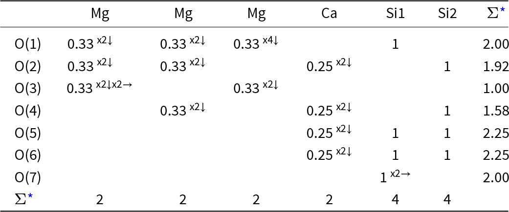
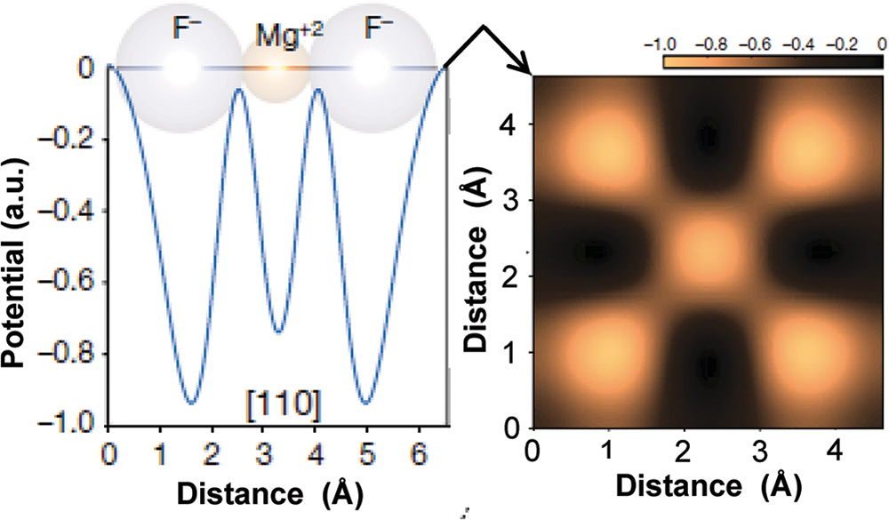
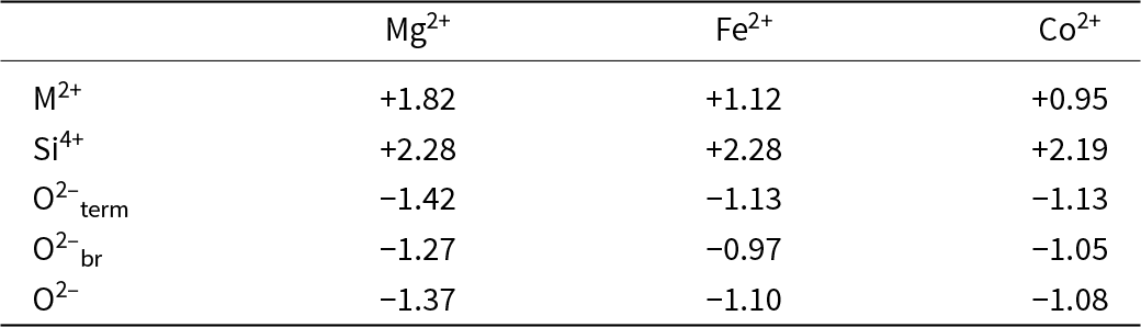
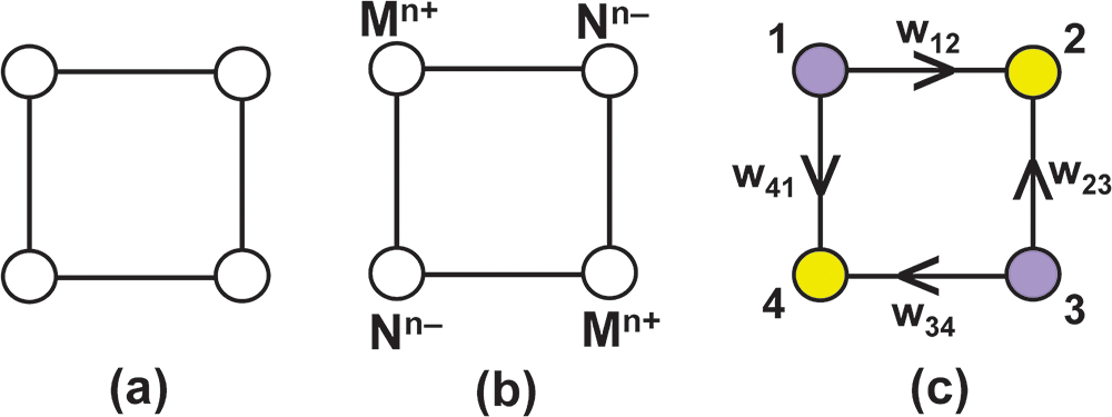
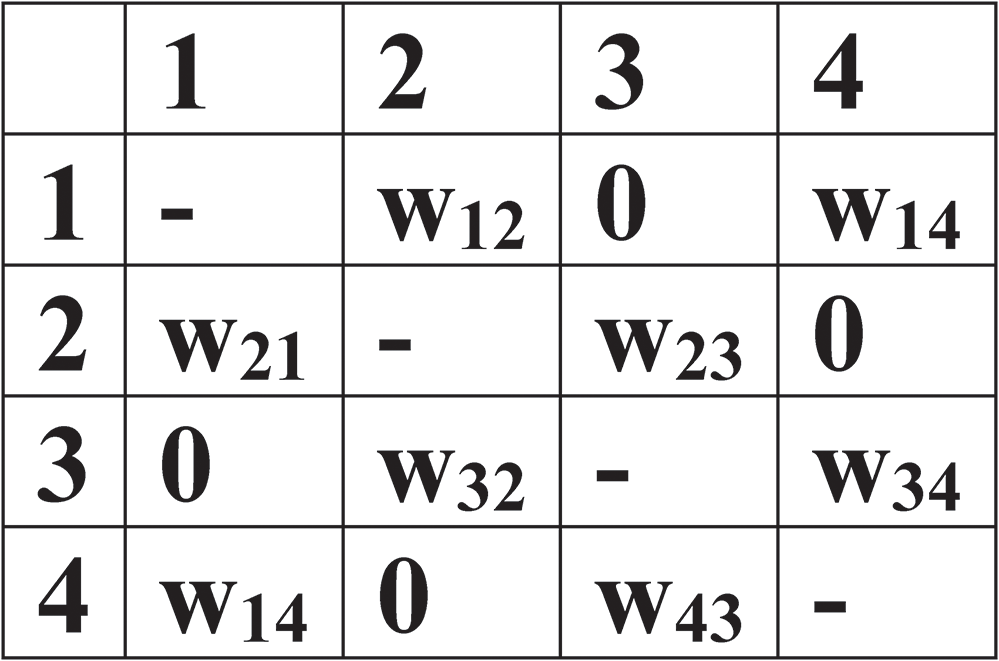
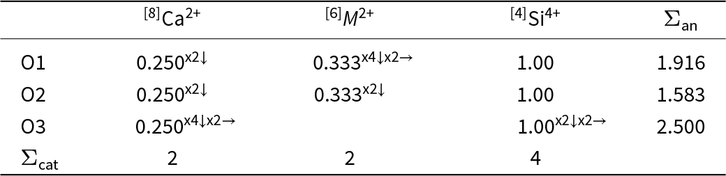
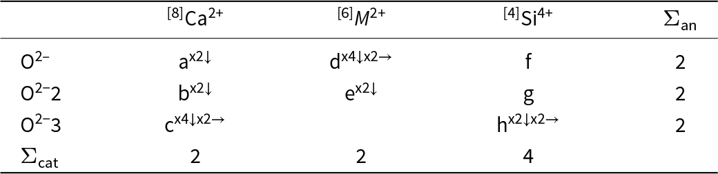
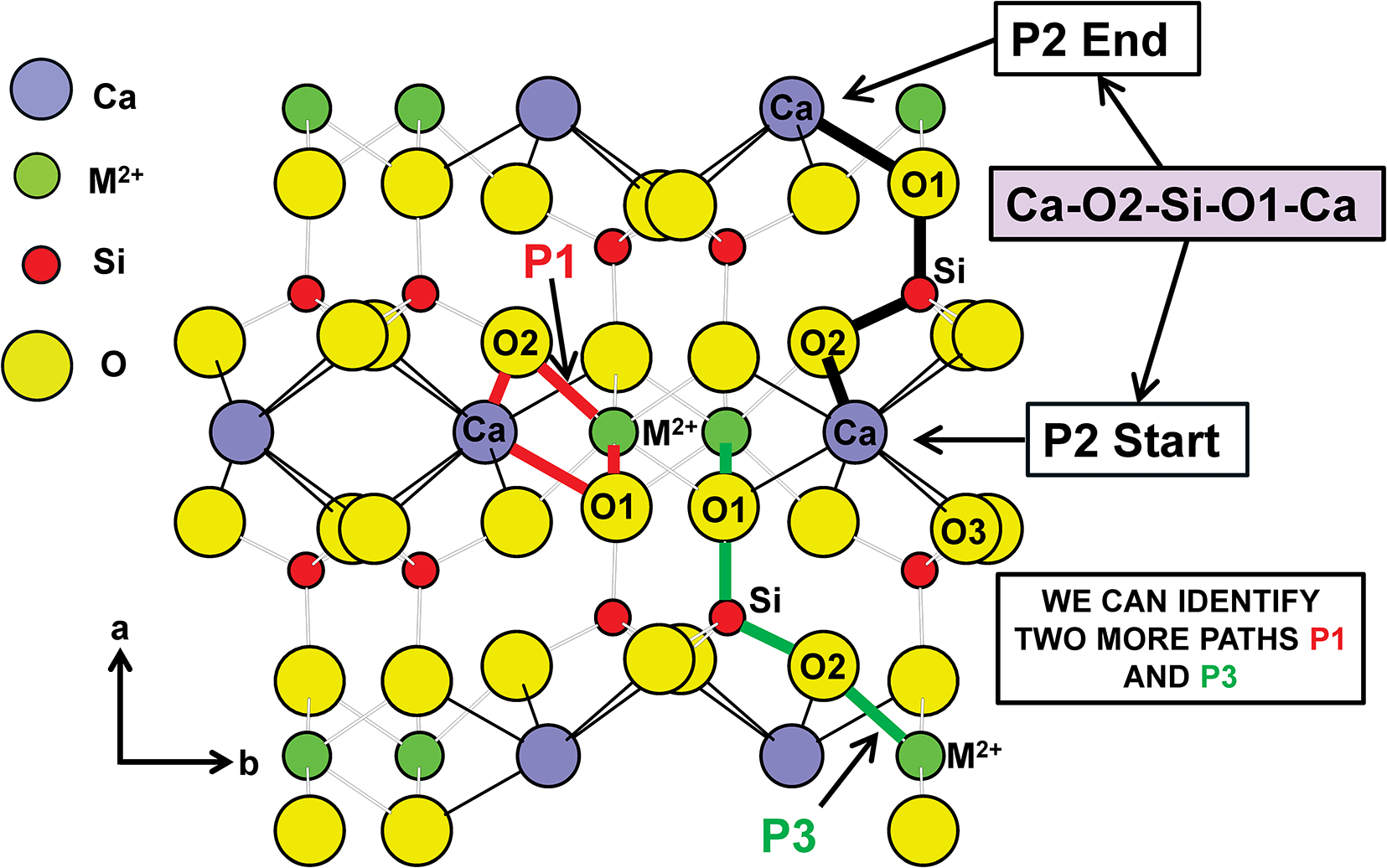
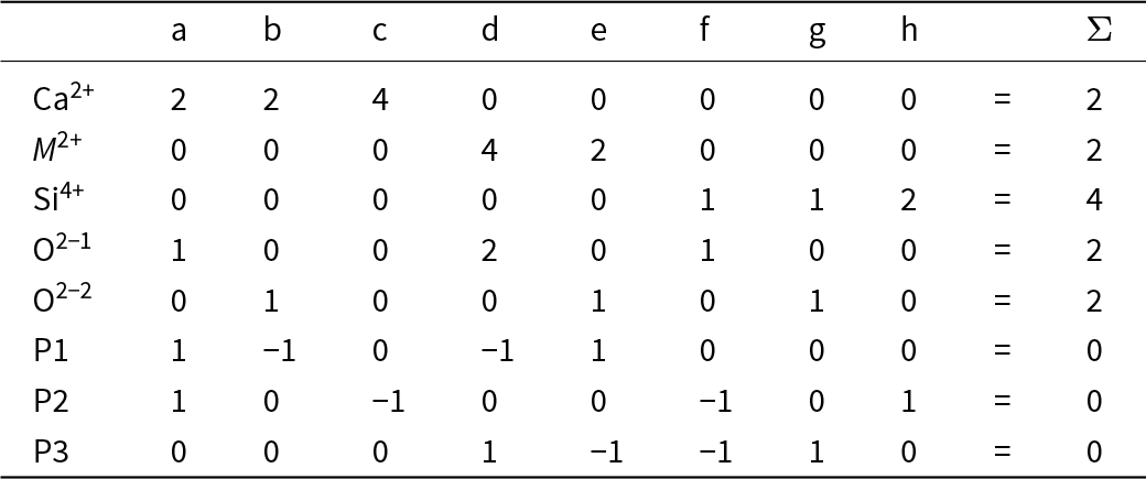
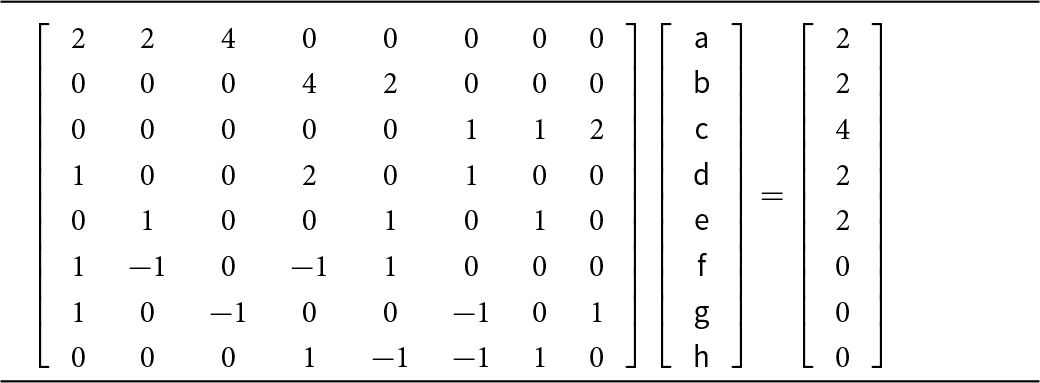
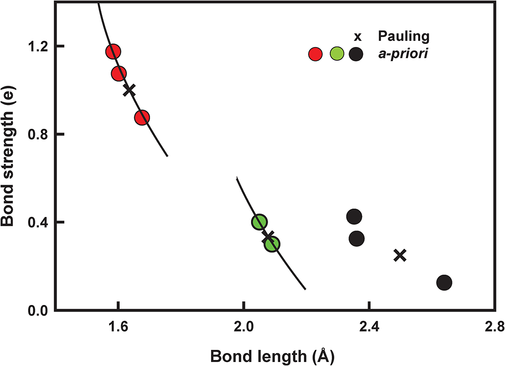
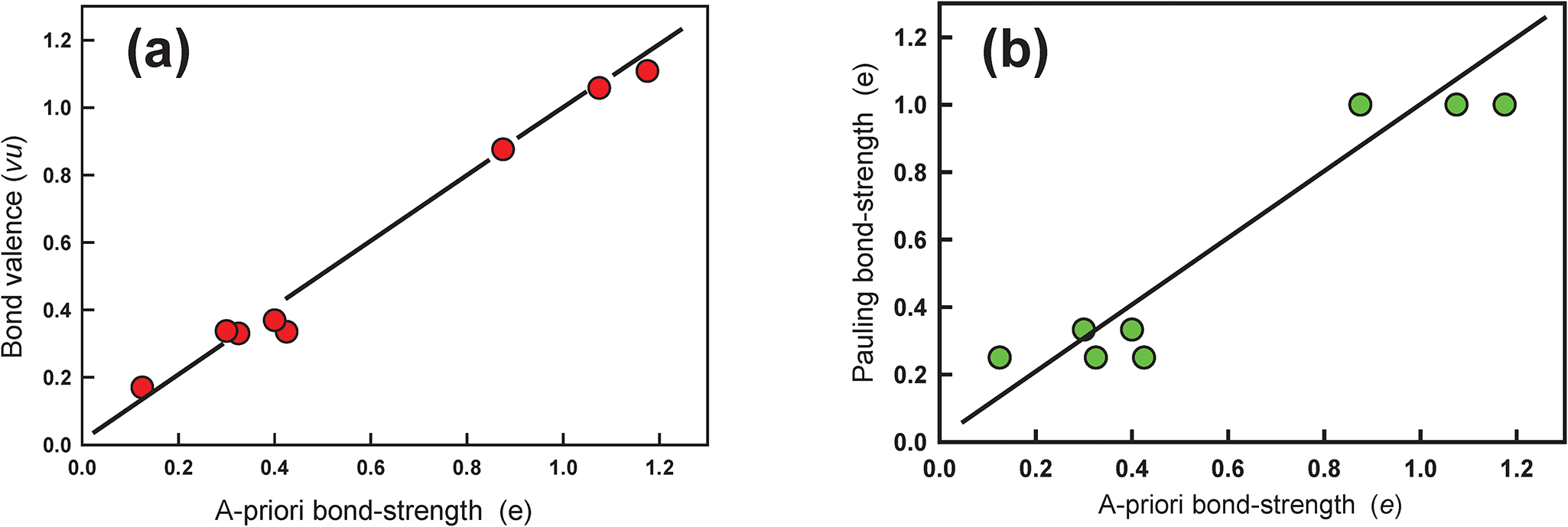
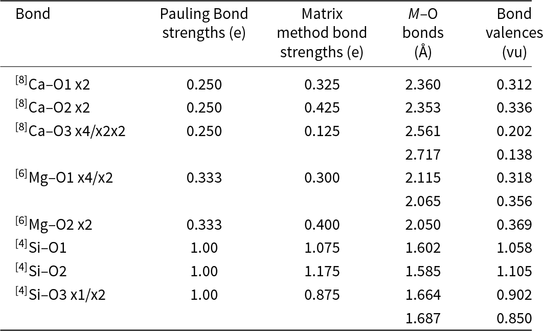
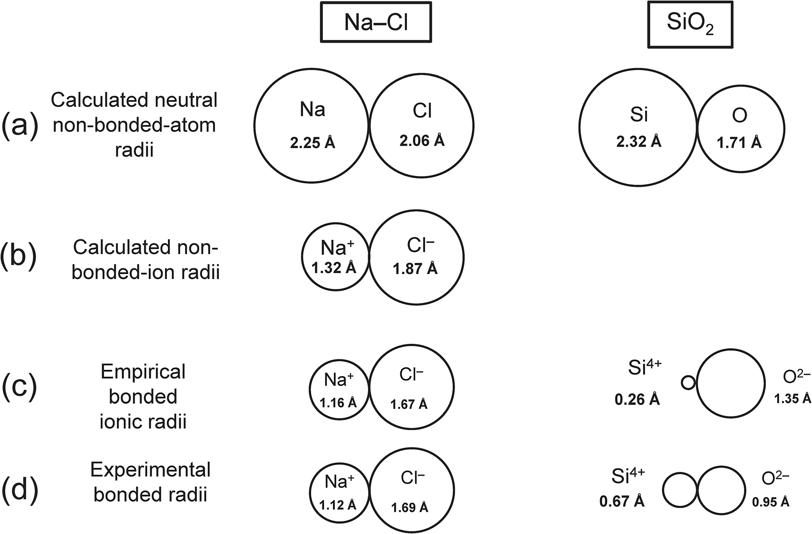
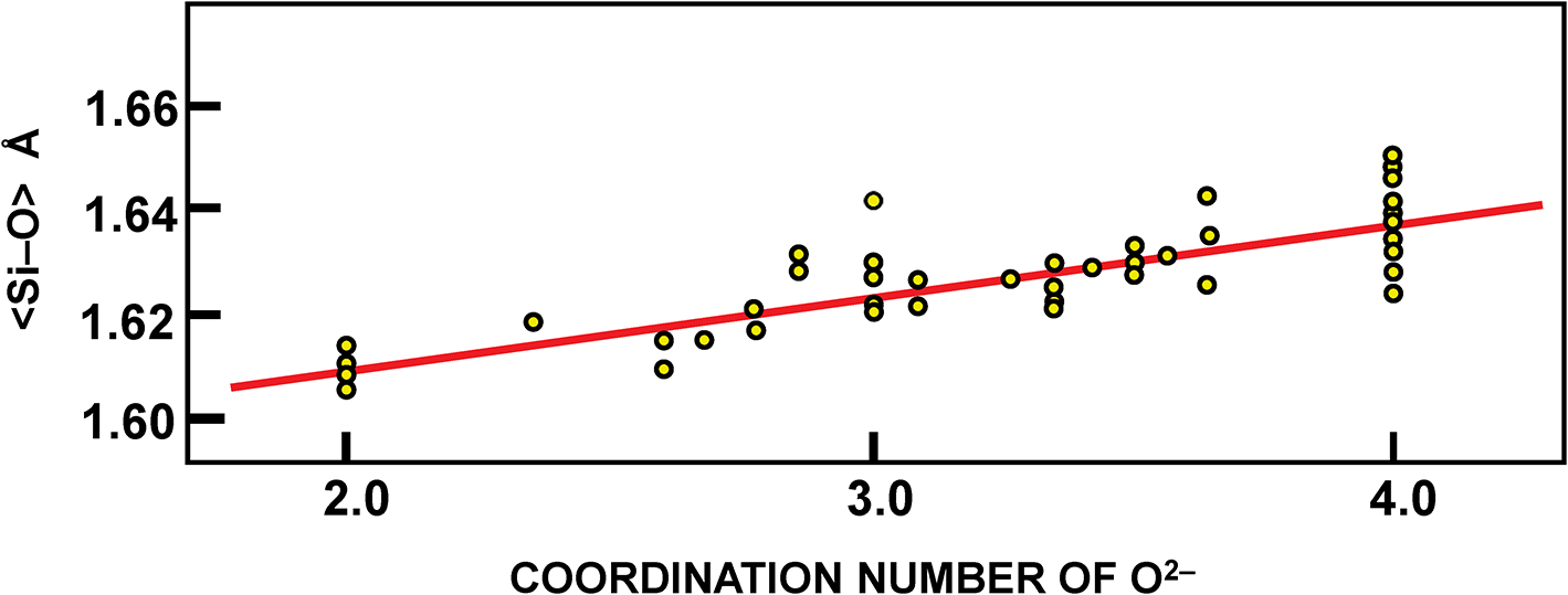
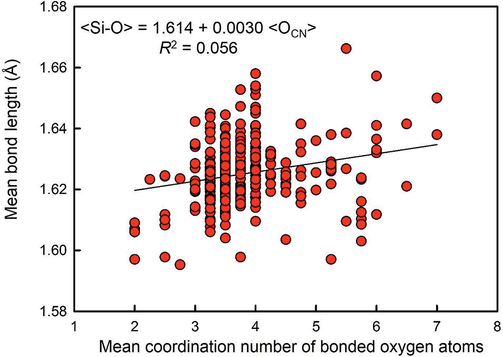
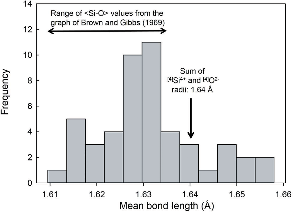
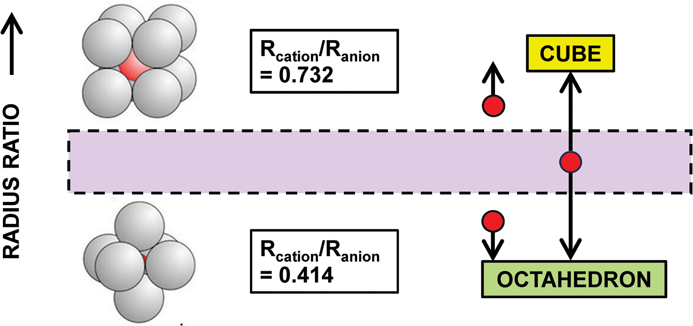
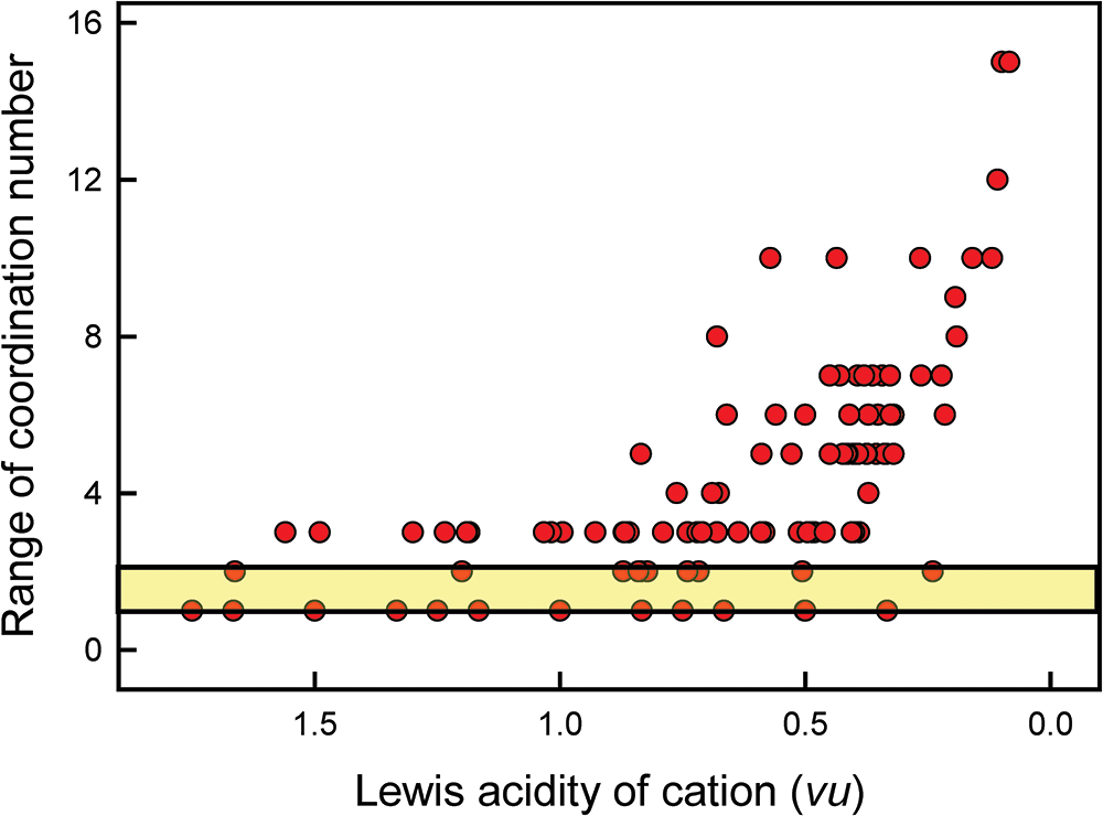
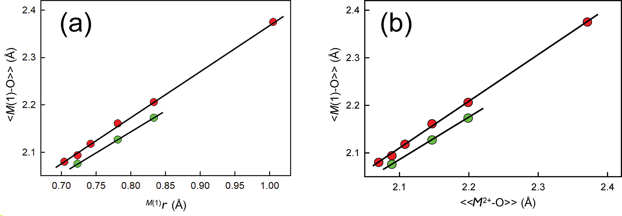
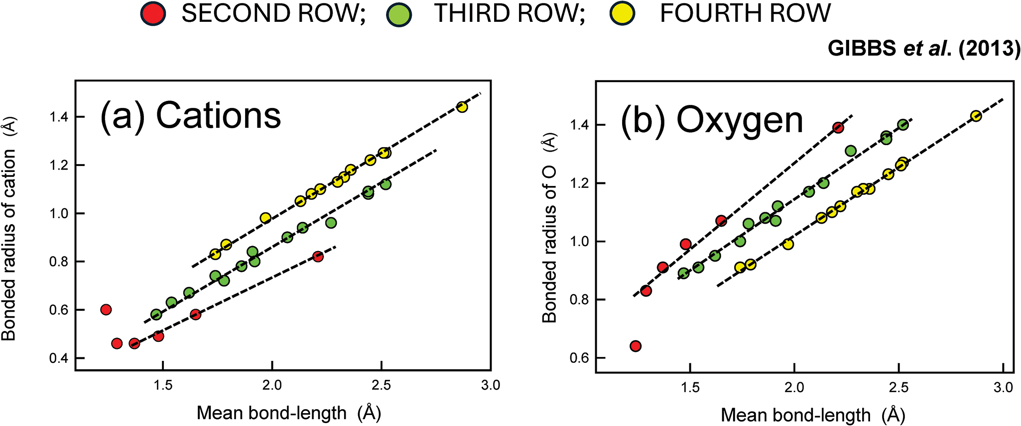
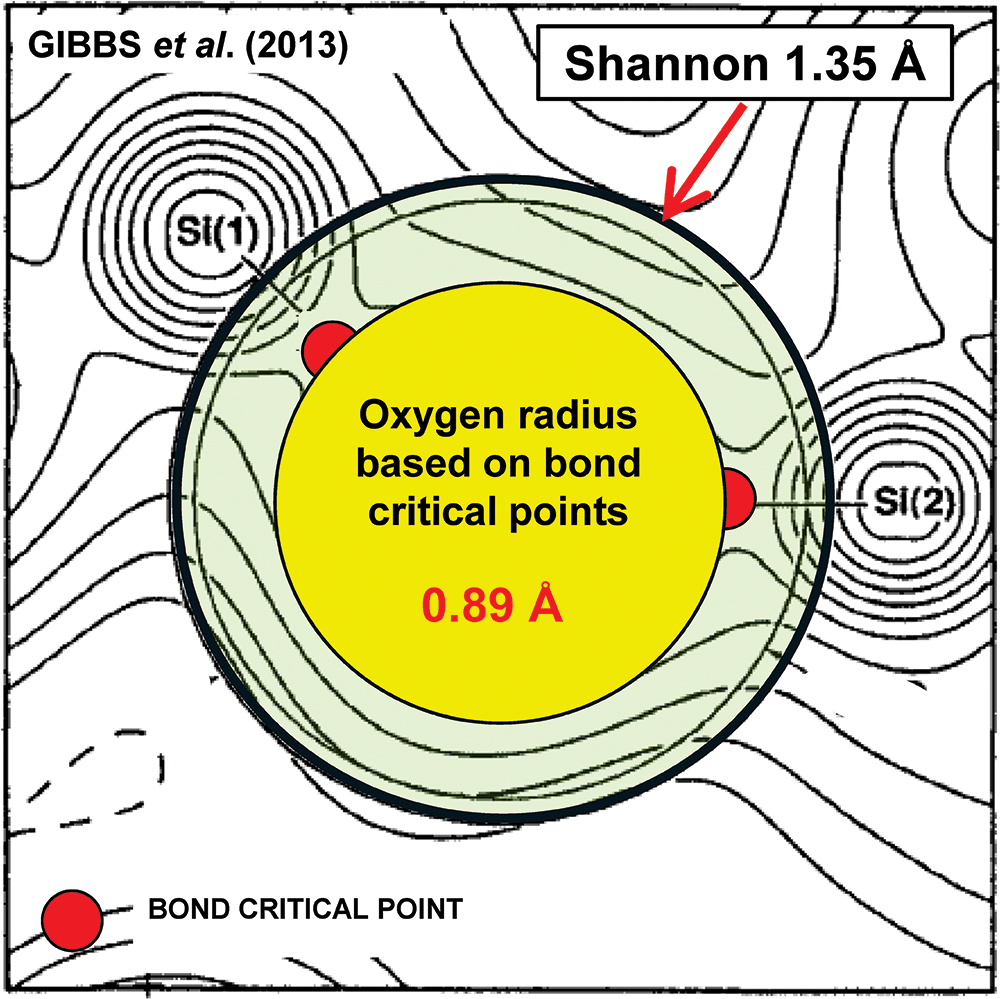
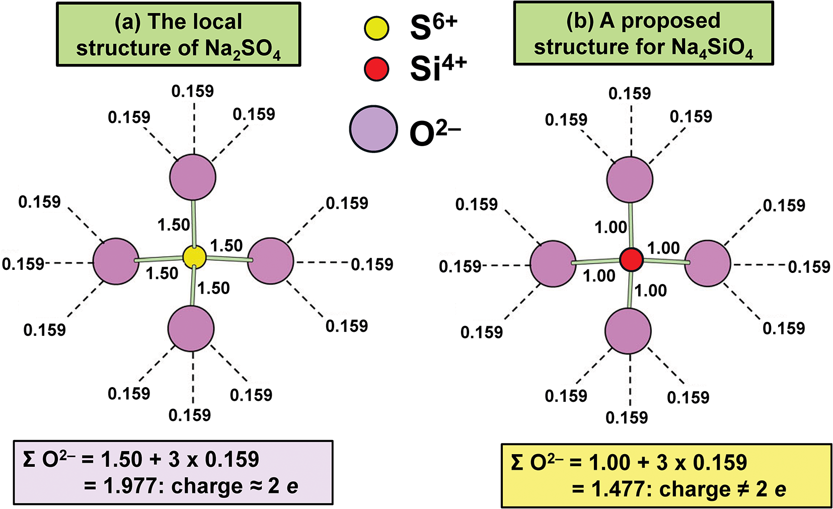
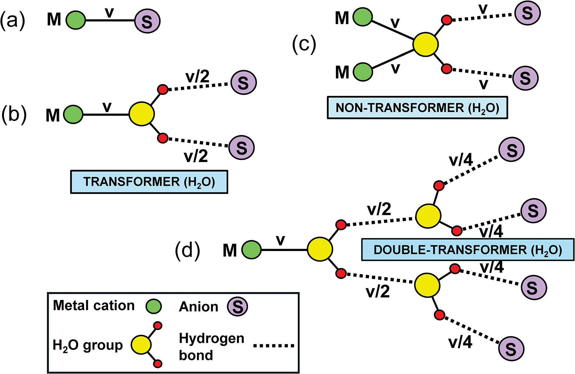
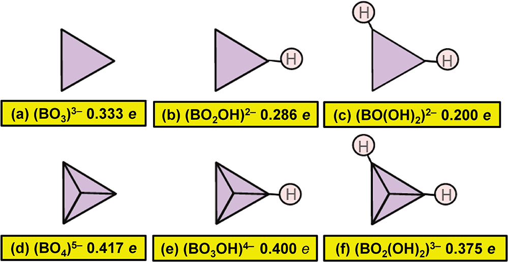
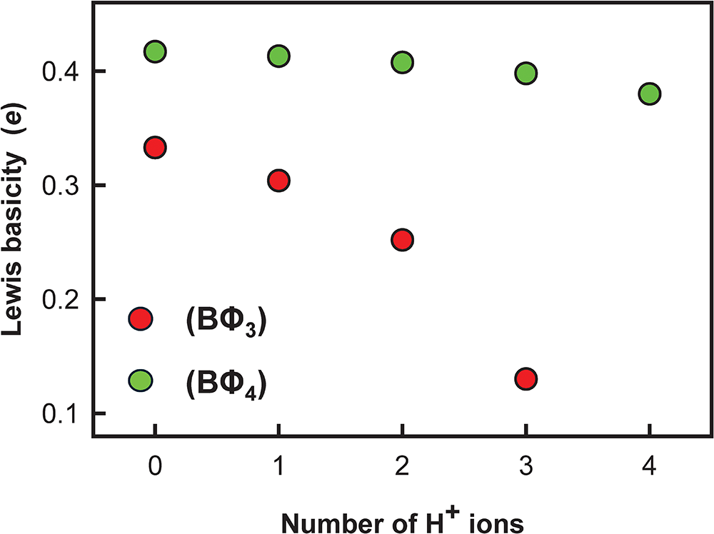
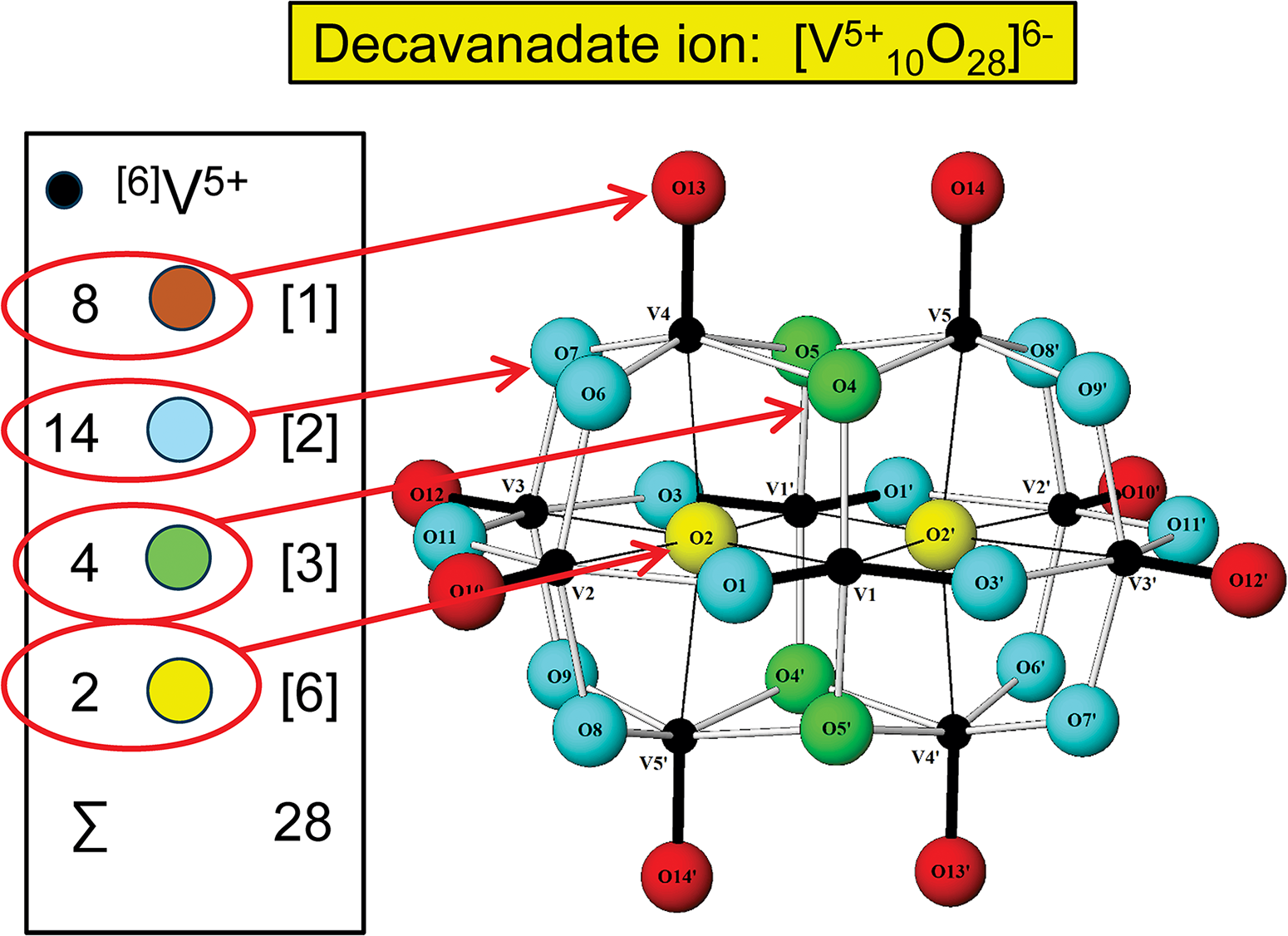
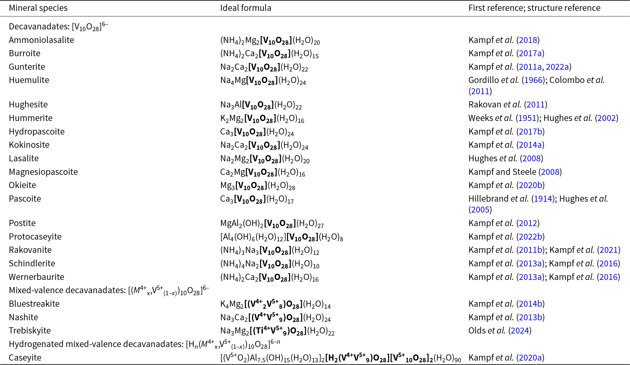
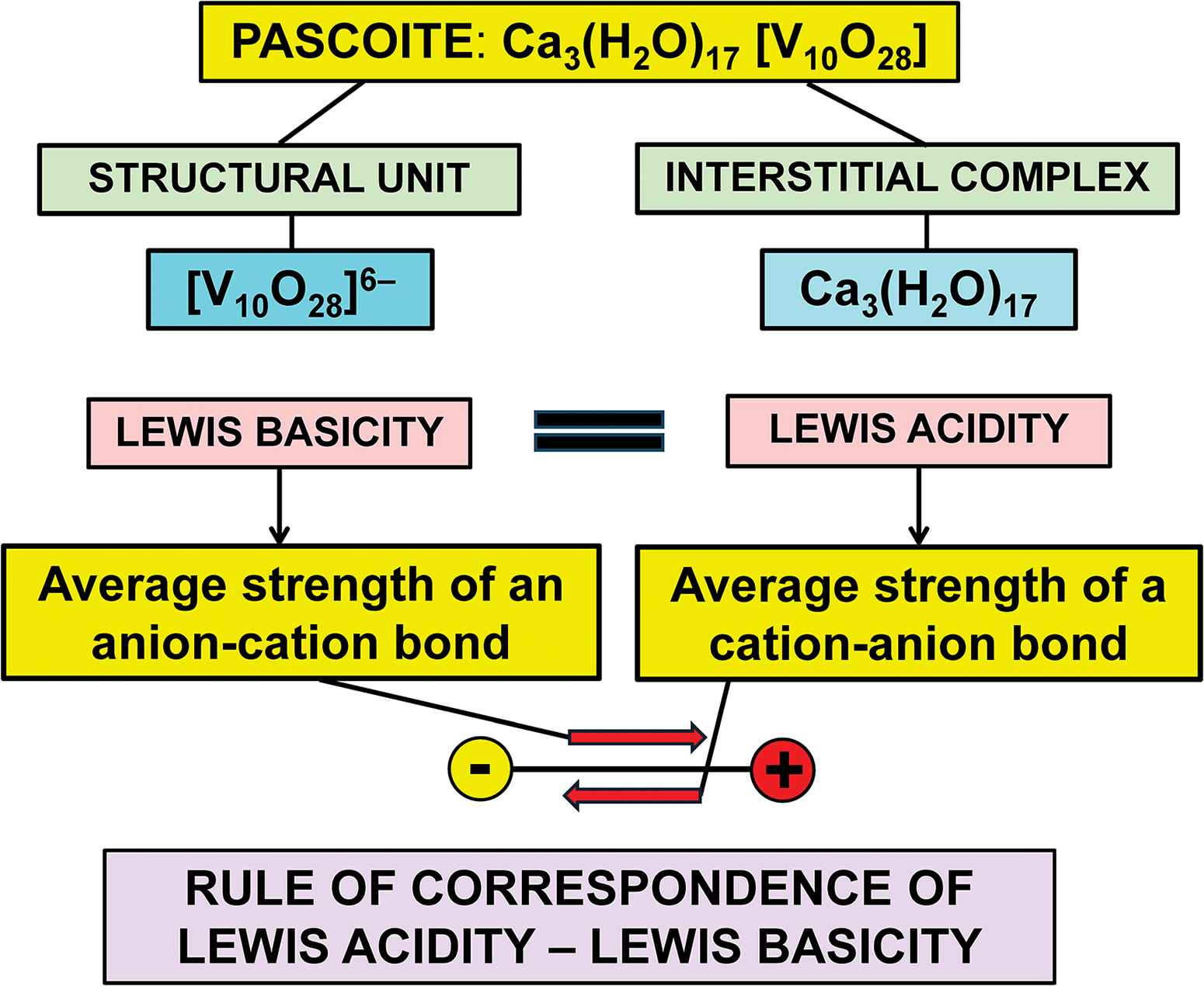
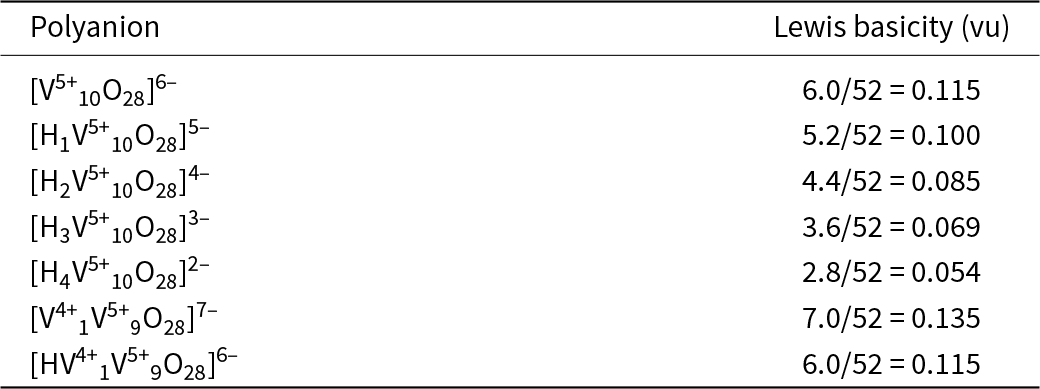
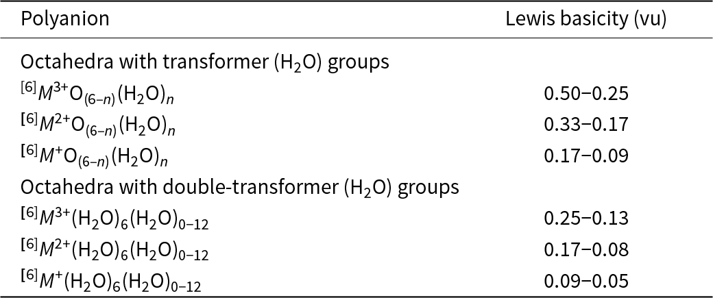
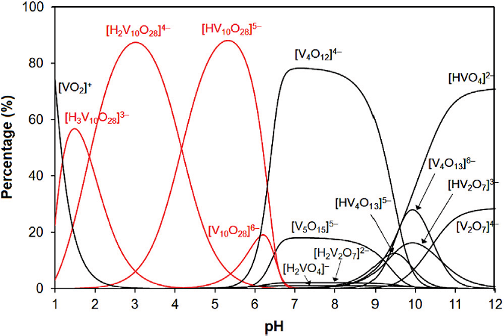

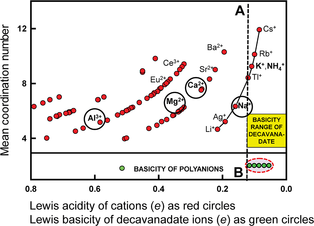
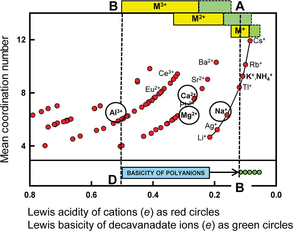
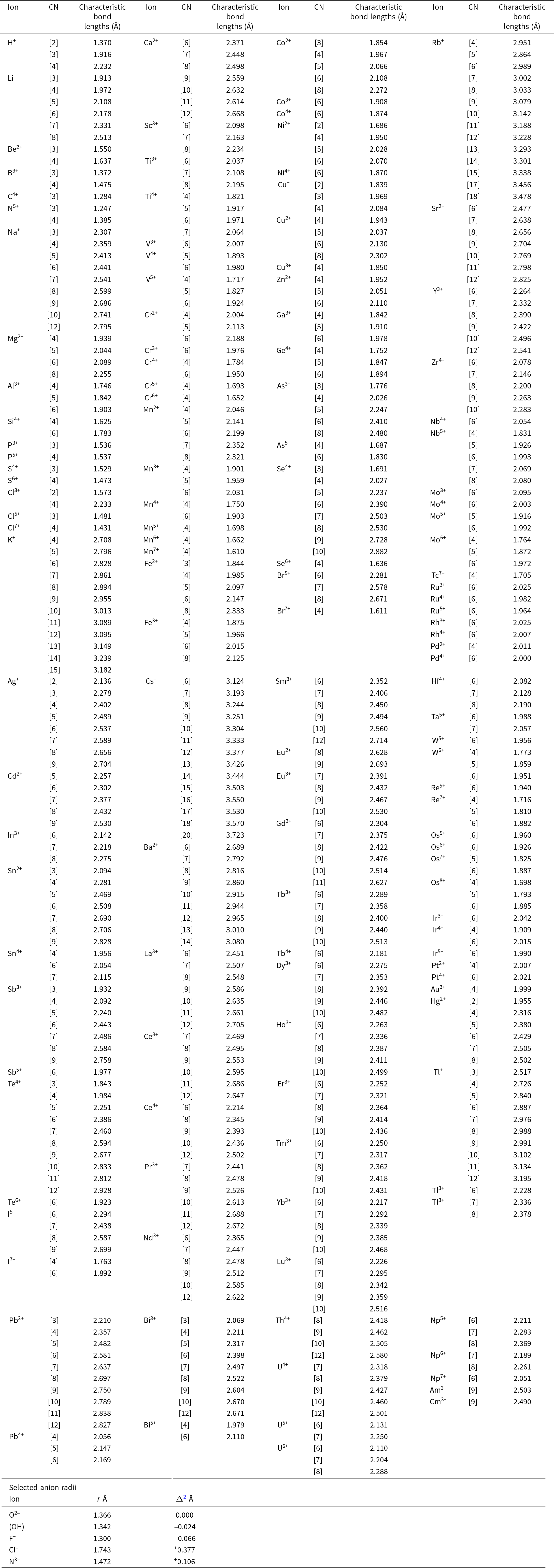
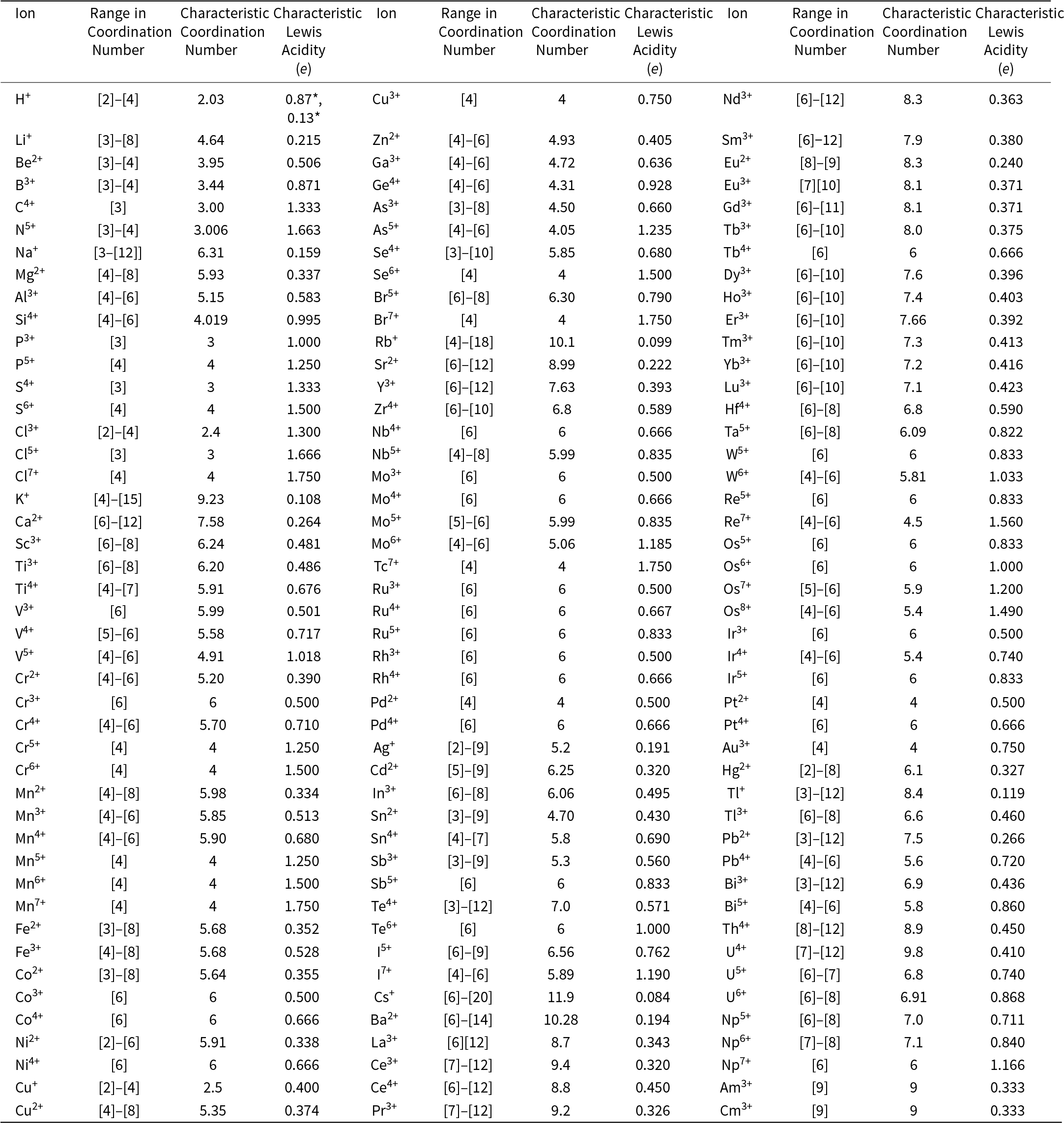
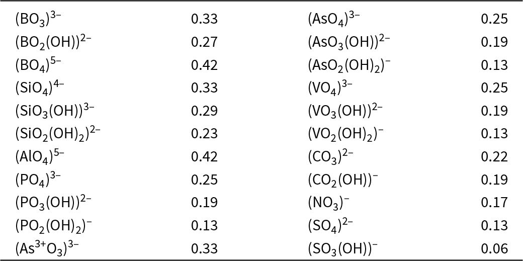

 Open access