

1. Introduction
Spurred by the Energy Independence and Security Act of 2007, the U.S. biofuel industry has experienced significant growth. So far, this growth in biofuel production has primarily occurred through corn-based ethanol. Currently, the corn ethanol industry has reached the annual minimum production capacity required to meet the “conventional” renewable fuel standard (RFS2) mandate (Renewable Fuel Association, 2015). This suggests that future growth in biofuel production may be met by alternative “advanced” feedstocks, including agricultural waste, biomass, and high sugar crops such as sugar beets, sugarcane, and sweet sorghum.
Sugar feedstocks are potential candidates among a number of feedstock pathways that are able to meet the RFS2 advanced biofuel mandates (Coyle, Reference Coyle2010; Linton et al., Reference Linton, Miller, Little, Petrolia and Coble2011; Outlaw et al., Reference Outlaw, Ribera, Richardson, da Silva, Bryant and Klose2007; Shapouri, Salassi, and Fairbanks, Reference Shapouri, Salassi and Fairbanks2006). Nonetheless, there are currently no commercial-scale sugar-based ethanol refineries in operation or construction in the United States. However, efforts are underway to develop energy beet ethanol refineries in North Dakota and California. The energy beet, a member of the beet family (Beta vulgaris), is a hybrid sugar beet that has been genetically engineered in various parts of the United States to yield sugar for ethanol production (McGrath and Townsend, Reference McGrath, Townsend, Cruz and Dierig2015; Wamisho, Ripplinger, and De Laporte, Reference Wamisho, Ripplinger and De Laporte2015). Although energy beets are specific to the United States, sugar beets are used in Europe for ethanol and sugar production.
The decision to invest in a new beet ethanol refinery is a dynamic process that is affected largely by ethanol price volatility, feedstock price, irreversible investments, and government policies. Because beet ethanol refinery investments have large sunk costs and the biorefinery is likely to operate in an uncertain market environment, potential investors have the option to delay investment decisions until additional price, cost, and policy information arises. The objective of this study is to assess the value of the opportunity to invest in a beet ethanol biorefinery and determine how the optimal decision rules for entry, mothballing, reactivation, and abandoning are affected by the volatilities of ethanol and beet prices and sunk costs. A real options value approach is used to estimate the ethanol gross margins that potentially trigger entry into and exit from the market.
Studies have evaluated the economic feasibility of ethanol investments in sugar-based feedstocks such as sweet sorghum, sugarcane, and sugar beets in the United States (Coyle, Reference Coyle2010; Linton et al., Reference Linton, Miller, Little, Petrolia and Coble2011; Maung and Gustafson, Reference Maung and Gustafson2011; Outlaw et al., Reference Outlaw, Ribera, Richardson, da Silva, Bryant and Klose2007; Rahmani and Hodges, 2006; Shapouri, Salassi, and Fairbanks, Reference Shapouri, Salassi and Fairbanks2006; Wamisho, Ripplinger, and De Laporte, Reference Wamisho, Ripplinger and De Laporte2015). However, all of these studies have used discounted cash flow techniques such as net present value (NPV) or break-even value analysis, methods that do not adequately account for managerial flexibility and the risk and uncertainty of future cash flows. The option valuation approach has become a preferred technique because it models decision makers’ flexible options to abandon, defer, or expand a project using new information (Dixit, Reference Dixit1989; Dixit and Pindyck, Reference Dixit and Pindyck1994).
The application of real options techniques to evaluate investment decisions in the U.S. ethanol industry has been limited in the past. However, notable applications of the real options approach (ROA) have evaluated investments in the U.S. biofuel industry (Cai and Stiegert, Reference Cai and Stiegert2014; Gallagher, Shapouri, and Brubaker, Reference Gallagher, Shapouri and Brubaker2007; Gonzalez, Karali, and Wetzstein, Reference Gonzalez, Karali and Wetzstein2012; Paulson et al., Reference Paulson, Babcock, Hart and Hayes2008; Pederson and Zou, Reference Pederson and Zou2009; Schmit, Luo, and Conrad, Reference Schmit, Luo and Conrad2011; Schmit, Luo, and Tauer, Reference Schmit, Luo and Tauer2009). Recently, a growing body of literature has analyzed key factors affecting ethanol investment decisions including government subsidy policies, economic factors, and strategic interactions in the ethanol industry sector in the United States, Canada, and Europe (Lade, Lin Lawell, and Smith, Reference Lade, Lin Lawell and Smith2016; Lin and Yi, Reference Lin and Yi2015; Schmit, Luo, and Conrad, Reference Schmit, Luo and Conrad2011; Thome and Lin Lawell, Reference Thome and Lin Lawell2015; Yi and Lin Lawell, Reference Yi and Lin Lawell2016; Yi, Lin, and Thome, Reference Yi, Lin and Thome2015). In terms of evaluating the effects of government policy on entry and exit decisions of corn ethanol plants, Schmit, Luo, and Conrad (Reference Schmit, Luo and Conrad2011) implemented ROA to evaluate how RFS policies affect the investment behavior of U.S. corn ethanol firms and decisions of industry entry and exit in the U.S. ethanol market. Yi, Lin, and Thome (Reference Yi, Lin and Thome2015) analyzed the effect of government subsidies including volumetric production, investment, and entry subsidies in U.S. fuel ethanol industry. Furthermore, Lade, Lin Lawell, and Smith (Reference Lade, Lin Lawell and Smith2016) developed a dynamic model of compliance based on a final enforcement ruling of RFS2 by the Environmental Protection Agency (EPA) and demonstrated how uncertainty about future relative fuel prices and changes in policy expectations can have dramatic effects on the price of compliance credits and ethanol production in the U.S. ethanol industry. For example, Lade, Lin Lawell, and Smith (Reference Lade, Lin Lawell and Smith2016, p. 28) found that the EPA's policy created uncertainty following the release of the 2014 Final Rule: “event day loss estimates range between $120 and $215 million, and increase over a two- and five-day horizon.” In addition, Thome and Lin Lawell (Reference Thome and Lin Lawell2015), Lin and Yi (Reference Lin and Yi2015), and Yi and Lin Lawell (Reference Yi and Lin Lawell2016) built a reduced form of discrete response and a structural econometric model of a dynamic game to analyze how economic factors, government policy, and strategic interactions affect timing and place of decisions to invest in ethanol plants in the United States, Canada, and Europe.
Studies outside the biofuel industry have addressed the following: the option to temporarily shut down (Brennan and Schwartz, Reference Brennan and Schwartz1985; McDonald and Siegel, Reference McDonald and Siegel1985); the option to continue or discontinue a planned investment (Majd and Pindyck, Reference Majd and Pindyck1987) and deferred investment (McDonald and Siegel, Reference McDonald and Siegel1985); the value of flexibility in alternative investment decisions, multistage projects, and switching options (Kulatilaka, Reference Kulatilaka1986; Trigeorgis, Reference Trigeorgis1996); and shutdown and upgrade decisions of wind turbine owners in Denmark based on a dynamic structural econometric model (Cook and Lin Lawell, Reference Cook and Lin Lawell2015).
The application of the ROA to beet ethanol investment analysis in this article makes several important contributions to the literature. First, the real options framework is applied to energy beet investors, allowing managerial flexibility to demonstrate how the uncertainty of ethanol and beet prices and sunk costs determine managerial behavior. Second, to date, no other study has applied real options analysis to beets or sugar-based ethanol in the Untied States. Most existing real options applications in the biofuel industry have been generally limited to investments that are already in operation and are largely on corn ethanol. In order to address these limitations, this study relies on a unique database that is created using a combination of information on beet prices and plant-level cost analysis. In particular, results from the investment analysis give valuable information to potential investors and policy makers, given that policy interests regarding biofuel industry expansion are shifting toward the development of advanced biofuel plants. Furthermore, the analysis helps to illustrate the importance of ethanol and beet price volatility, sunk costs, and uncertainty, given that shutdown and temporary mothballing of active plants have been commonplace in the corn ethanol industry since late 2007 (Hertel and Beckman, Reference Hertel, Beckman, Graff Zivin and Perloff2012; Wisner, Reference Wisner2009), largely as a result of high feedstock prices and declining ethanol prices. For example, following the 2008 financial crisis, approximately 12% of the formerly operating production capacity was shut down (Wisner, Reference Wisner2009). At that time, about 15 to 18 plants were under construction but temporarily halted construction because of adverse economic conditions (Wisner, Reference Wisner2009). In 2013, out of 211, nearly 10% of ethanol plants temporarily suspended production as the 2012 drought tightened corn supply and the subsequent high corn prices made producing ethanol too expensive.
This study is based on a standard ROA and exposition of Dixit and Pindyck (Reference Dixit and Pindyck1994). The methodological framework and some of the parametric assumptions follow from Schmit, Luo, and Tauer (Reference Schmit, Luo and Tauer2009) and Schmit, Luo, and Conrad (Reference Schmit, Luo and Conrad2011). To investigate the significance of the approach, this article develops a real options model to examine the basis for firms’ entry and exit decisions and compares these trigger gross margins with break-even entry and exit gross margins to determine a price premium for risk and uncertainty. Sensitivity analysis on a range of possible ethanol gross margin volatility parameters, and sunk costs, is then conducted to explore how firm investment behavior is affected by a change in these parameters. The effect of managerial flexibility on the entry risk premiums and gross margins of ethanol that trigger mothballing, reactivation, and exit are also discussed. This article also evaluates hysteresis, the range of inaction in firm behavior that may arise as a result of the uncertainty in future gross margin values and irreversible investment. The investment analysis relies on the economics of a beet ethanol refinery facing typical market conditions in the northern plains of the United States. The empirical analysis is based on historical monthly ethanol and beet prices from 2000 to 2014 and recent surveys of operating and capital costs. We take historical sugar beet prices as a proxy for energy beet price, assuming that sugar beet prices can represent the future price of energy beets given that both crops have similar agronomic attributes and require the same cultural and management practices.
The next section develops the conceptual model for optimal entry, mothballing, reactivation, and exit. Then, Section 3 covers how data and stochastic-process parameters are constructed. The empirical results are elucidated in Section 4, and Section 5 discusses the conclusions and implications of the study, guides for policy development, and directions for future research.
2. Conceptual Framework and Empirical Specification
The standard NPV investment decision rule is based on the Marshallian concept of the theory of entry and exit. The argument, under NPV assumptions, is that a firm will invest/enter in a specific market if the discounted net return is greater than or equal to the discounted operating cost plus capital expenditures. A firm will exit the market if the discounted net return falls below the discounted operating cost plus the net scrap value of selling the plant. The drawbacks of this methodology are that it ignores the opportunity cost of waiting for new information and assumes that future cash flows follow a constant pattern that can be accurately predicted. In effect, the NPV approach is not flexible when an investment is irreversible and the decision to invest can be postponed (Dixit, Reference Dixit1989; Dixit and Pindyck, Reference Dixit and Pindyck1994; Pindyck, Reference Pindyck1991).
2.1. Entry and Exit Strategies under Uncertainty: A Conceptual Framework
There are three different states in which an ethanol refinery can be and five multiple switching options. The refinery states are idle, active, or mothballed. The switching options are idle to active, active to mothballed, mothballed to active, mothballed to exit (abandoned), and active to exit. The switching options this study evaluates include the following: (1) idle to active, (2) active to mothballed, (3) mothballed to active, and (4) active to exit.
In an idle state, a firm does not pay fixed or capital costs because the plant has not yet been built. An idle firm will invest when the demand conditions for output become sufficiently favorable, and an active firm will abandon the plant if demand becomes sufficiently adverse (Dixit and Pindyck, Reference Dixit and Pindyck1994). In this study, we assume that the firm incurs a lump-sum fixed cost K to invest in an energy beet ethanol refinery. If the refinery decides to shut down (exit), there is a lump-sum exit/abandonment cost l to close it. A refinery can recoup part of the investment cost K upon exit, reflecting that part of K is not fully sunk. Once the investment is made, the refinery generates a given flow of ethanol production until the plant is shut down. A refinery firm incurs a constant operating cost of ω to produce each unit of output. The ethanol refinery will generate a flow of operating profit equal to P − ω per period, where P is the firm's ethanol gross margin (dollars per gallon). The ethanol gross margin is defined as the sum of ethanol and beet pulp prices minus beet price. The nonbeet operating cost (ω) is the sum of all operating costs less beet feedstock cost (dollars per gallon). Two possibilities exist: the ethanol refinery may be shut down if P < ω and later reactivated if P > ω. This makes the ethanol refinery have an infinite sequence of instantaneous operating options, each of which is exercised if P > ω and can be valued accordingly (Dixit and Pindyck, Reference Dixit and Pindyck1994). Instead of abandoning, an ethanol refinery may choose to suspend operations and mothball, then later reactivate. In a mothballed state, a firm incurs an ongoing maintenance cost, m, to maintain existing capital. Mothballing requires a sunk cost per unit of expected output, Em . In addition, the refinery can be reactivated in the future at an additional sunk cost, r. Finally, we assume m < ω for the mothballing option to be feasible.
The key variables to the investment decision in this particular investment analysis are ethanol gross margin and investment costs. The decisions to invest and exit are made assuming that the gross margin of ethanol is exogenous and stochastic and that it evolves according to geometric Brownian motion (GBM), described in equation (1):
 $$\begin{equation}
dP = \mu Pdt + \sigma Pdz,
\end{equation}$$
$$\begin{equation}
dP = \mu Pdt + \sigma Pdz,
\end{equation}$$
where P is the gross margin of the refinery, μ is an instantaneous drift in the gross margins of ethanol, σ is the standard deviation or volatility of a given random increment to the gross margins of ethanol, and dz is an increment to the standard Wiener processes for the uncertain variable and is uncorrelated across time t and $dz = \sigma \sqrt {\Delta t} $
, E[dz
2] = dt.
$dz = \sigma \sqrt {\Delta t} $
, E[dz
2] = dt.
2.1.1. The Decision to Enter
The conceptual framework and the mathematical derivations of entry and exit decisions in this section are adapted from Dixit and Pindyck (Reference Dixit and Pindyck1994) and Schmit, Luo, and Tauer (Reference Schmit, Luo and Tauer2009) and Schmit, Luo, and Conrad (Reference Schmit, Luo and Conrad2011). We assume that the value of a project is a function of the exogenous state variable (i.e., the gross margin of ethanol). Let V 0(P)be the discounted expected value of an idle project or the option to invest. Similarly, V 1(p) is the value for the active project. The solution consists of these functions and the rules for optimally switching between idle and active states. If the investors “sold” the refinery instead of deciding to invest, they would earn V 0(P). Equilibrium in the asset market requires that
 $$\begin{equation}
\delta {V_0}(P) = \frac{{{E_t}[d{V_0}(p)]}}{{dt}},
\end{equation}$$
$$\begin{equation}
\delta {V_0}(P) = \frac{{{E_t}[d{V_0}(p)]}}{{dt}},
\end{equation}$$
where P is the gross margin of ethanol, δ is the discount rate, δV
0(P) represents the normal return if the option to invest is sold, and $\frac{{{E_t}[d{V_0}(p)]}}{{dt}}$
is the expected capital gain from holding the option to invest. Equation (2) defines the entry trigger gross margin.
$\frac{{{E_t}[d{V_0}(p)]}}{{dt}}$
is the expected capital gain from holding the option to invest. Equation (2) defines the entry trigger gross margin.
From Ito's lemma, for a function V = V 0(P),
 $$\begin{equation}
dV = [V(P) + \mu P{V'_0}(P) + 0.5{P^2}{V''_0}(P){\sigma ^2}]dt + \sigma P{V'_0}(P)dZ,
\end{equation}$$
$$\begin{equation}
dV = [V(P) + \mu P{V'_0}(P) + 0.5{P^2}{V''_0}(P){\sigma ^2}]dt + \sigma P{V'_0}(P)dZ,
\end{equation}$$
where μ and σ are respectively the drift and standard deviation parameters of P; ${V_t} = {{\partial V} / {\partial t}} = 0$
, given the infinite time horizon,
${V_t} = {{\partial V} / {\partial t}} = 0$
, given the infinite time horizon, ${V'_0} = {{\partial V} / {\partial P}}$
,
${V'_0} = {{\partial V} / {\partial P}}$
, ${V''_0} = {{{\partial ^2}V} / {\partial {P^2}}},$
and E[dZ] = 0. Simplifying equation(3) and substituting into equation(2) gives us the asset equilibrium condition represented by the differential equation:
${V''_0} = {{{\partial ^2}V} / {\partial {P^2}}},$
and E[dZ] = 0. Simplifying equation(3) and substituting into equation(2) gives us the asset equilibrium condition represented by the differential equation:
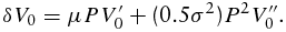 $$\begin{equation}
\delta {V_0} = \mu P{V'_0} + (0.5{\sigma ^2}){P^2}{V''_0}.
\end{equation}$$
$$\begin{equation}
\delta {V_0} = \mu P{V'_0} + (0.5{\sigma ^2}){P^2}{V''_0}.
\end{equation}$$
The general solution for an idled firm for this homogenous second-order ordinary differential equation gives us:
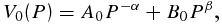 $$\begin{equation}
{V_0}(P) = {A_0}{P^{ - \alpha }} + {B_0}{P^\beta },
\end{equation}$$
$$\begin{equation}
{V_0}(P) = {A_0}{P^{ - \alpha }} + {B_0}{P^\beta },
\end{equation}$$
where A 0 and B 0 are unknown constants to be determined, and α and β are the root mean of the quadratic equation parameters that capture and incorporate the uncertainty modeled by GBM into the model:
 $$\begin{equation*}
\beta = \frac{{(1 - m) + {{[{{(1 - m)}^2} + 4g]}^{1/2}}}}{2} > 0
\end{equation*}$$
$$\begin{equation*}
\beta = \frac{{(1 - m) + {{[{{(1 - m)}^2} + 4g]}^{1/2}}}}{2} > 0
\end{equation*}$$
 $$\begin{equation*}- \alpha = \frac{{(1 - m) - {{[{{(1 - m)}^2} + 4g]}^{1/2}}}}{2} < 0
\end{equation*}$$
$$\begin{equation*}- \alpha = \frac{{(1 - m) - {{[{{(1 - m)}^2} + 4g]}^{1/2}}}}{2} < 0
\end{equation*}$$
where m = 2μσ−2 and g = 2δσ−2, and for the convergence condition, g > m implies that δ > μ; δ is the discount rate. A 0 P −α and B 0 P β capture the option value of switching to another state if margin P changes. An idle project has no value if P approaches zero; if A 0 P −αapproaches zero, the first term in equation (5) vanishes. Because –α < 0 and β > 1, this requires A 0 = 0 and simplifies equation(5), which gives the following solution to the differential equation:
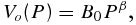 $$\begin{equation}
{V_o}(P) = {B_0}{P^\beta },
\end{equation}$$
$$\begin{equation}
{V_o}(P) = {B_0}{P^\beta },
\end{equation}$$
where Vo (P) is the value function of an idle investment and can be interpreted as the value of the option to enter.
2.1.2. The Decision to Mothball
If the gross margin of ethanol falls below ω, instead of permanently abandoning the refinery, the refinery owner has the option to put the refinery into a state of temporary suspension, allowing it to be reactivated in the future at a sunk cost that is much less than the cost of building a new refinery.
Consider a refinery that is operating and earning instantaneous net revenue (p – ω). Let V 1(p) denote the value function of the active refinery. Equilibrium conditions require that
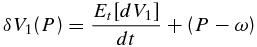 $$\begin{equation}
\delta {V_1}(P) = \frac{{{E_t}[d{V_1}]}}{{dt}} + (P - \omega )
\end{equation}$$
$$\begin{equation}
\delta {V_1}(P) = \frac{{{E_t}[d{V_1}]}}{{dt}} + (P - \omega )
\end{equation}$$
where V 1(p) is the value function of an active refinery, and ω is the operating cost. The left-hand side is the normal return if the refinery is sold and proceeds invested at discount rate δ. The right-hand side of equation (7) is the net revenue flow plus the expected capital gain. The derivation of the value of the active firm is done in a similar way to the idle firm, except that an active firm receives the flow of operating profit (P − ω)dt, in addition to the expected capital gain. The general solution for an active refinery can be expressed as follows:
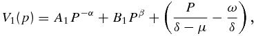 $$\begin{equation}
{V_1}(p) = {A_1}{P^{ - \alpha }} + {B_1}{P^\beta } + \left(\frac{P}{{\delta - \mu }} - \frac{\omega }{\delta }\right),
\end{equation}$$
$$\begin{equation}
{V_1}(p) = {A_1}{P^{ - \alpha }} + {B_1}{P^\beta } + \left(\frac{P}{{\delta - \mu }} - \frac{\omega }{\delta }\right),
\end{equation}$$
where A 1 and B 1 are unknown constants to be determined, A 1 P −α + B 1 P β captures the option value of the mothballed refinery, and P(δ − μ)−1 − ωδ−1 is the present value of the net cash flow. The value of the mothballing option goes to zero as P gets very large, implying that B 1 = 0. Therefore, equation (8) becomes
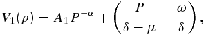 $$\begin{equation}
{V_1}(p) = {A_1}{P^{ - \alpha }} + \left(\frac{P}{{\delta - \mu }} - \frac{\omega }{\delta }\right),
\end{equation}$$
$$\begin{equation}
{V_1}(p) = {A_1}{P^{ - \alpha }} + \left(\frac{P}{{\delta - \mu }} - \frac{\omega }{\delta }\right),
\end{equation}$$
where A 1 P −α represents the value of the option to mothball and P(δ − μ)−1 − ωδ−1 captures the expected present value of continuing production forever. The value of the mothballing option is derived from future possibilities of reactivation or abandonment. Note that an economically meaningful solution for V 0 must be nonnegative. Therefore, we must haveB 1 ⩾ 0 in equation (8). Similarly, an active firm has an expected value of P(δ − μ)−1 − ωδ−1 from the feasible strategy of never shutting down. Also, in equation (9), we must haveA 1 ⩾ 0 (Dixit, Reference Dixit1989).
2.1.3. The Decision to Reactivate and Exit
Mothballing requires a sunk cost, Em . In a mothballed state, the refinery requires maintenance at a cost of m. Let Vm (p) denote the value function of the mothballed refinery with the option of reactivating or exiting. Equilibrium in the asset market requires that
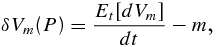 $$\begin{equation}
\delta {V_m}(P) = \frac{{{E_t}[d{V_m}]}}{{dt}} - m,
\end{equation}$$
$$\begin{equation}
\delta {V_m}(P) = \frac{{{E_t}[d{V_m}]}}{{dt}} - m,
\end{equation}$$
where the left-hand side is the normal return if the firm sells the mothballed refinery and invests the earnings at the discount rate of δ, and the right-hand side is the expected capital gain of the mothballed refinery less ongoing maintenance costs. The resulting value function can be expressed as follows:
 $$\begin{equation}
{V_m}(p) = {A_m}{P^{ - \alpha }} + {B_m}{P^\beta } - m{\delta ^{ - 1}},
\end{equation}$$
$$\begin{equation}
{V_m}(p) = {A_m}{P^{ - \alpha }} + {B_m}{P^\beta } - m{\delta ^{ - 1}},
\end{equation}$$
where Am and Bm are constants to be determined, AmP −α is the value of the option to reactivate the mothballed refinery, BmP βis the value of the option to exit, and mδ−1 is the capitalized maintenance cost assuming that the refinery remains in the mothballed state forever. Mothballing only makes sense if the maintenance cost (m) is less than the cost of actual operation and if the reactivation cost is less than the cost of reinvesting. The option value to exit is positive only if the gross margin decreases, and the option value to reactivate is positive only if the gross margin increases.
2.1.4. Deriving Trigger Gross Margin
For our representative ethanol refinery, four switching options are considered: from idle to active, active to mothballed, mothballed to active, and active to exit (abandon). At each switching option point, the value-matching and smooth-pasting conditions must hold. Each of these options will be exercised at a specific gross margin value. Smooth-pasting conditions require tangency of the value functions at the respective trigger gross margins.
For the active investment option, the value-matching and smooth-pasting conditions are, respectively,
 $$\begin{equation}
{V_o}({P_h}) = {V_1}({P_h}) - K \quad {\rm{and}}\quad {V^\prime_o}({P_h}) = {V^\prime_1}({P_h}),
\end{equation}$$
$$\begin{equation}
{V_o}({P_h}) = {V_1}({P_h}) - K \quad {\rm{and}}\quad {V^\prime_o}({P_h}) = {V^\prime_1}({P_h}),
\end{equation}$$
where Ph is the real options entry trigger gross margin. For mothballing, the value-matching and smooth-pasting conditions are, respectively,
 $$\begin{equation}
{V_1}({P_m}) = {V_m}({P_m}) - {E_m}\quad {\rm{and}}\quad {V^\prime_1}({P_m}) = {V^\prime_m}({P_m}),
\end{equation}$$
$$\begin{equation}
{V_1}({P_m}) = {V_m}({P_m}) - {E_m}\quad {\rm{and}}\quad {V^\prime_1}({P_m}) = {V^\prime_m}({P_m}),
\end{equation}$$
where Vm (P) is the value function of the mothballed refinery, and Pm is the real options mothball trigger gross margin. For reactivation, the value-matching and smooth-pasting conditions are, respectively,
 $$\begin{equation}
{V_m}({P_r}) = {V_1}({P_r}) - r\quad {\rm{and}}\quad {V'_m}({P_r}) = {V'_1}({P_r}),
\end{equation}$$
$$\begin{equation}
{V_m}({P_r}) = {V_1}({P_r}) - r\quad {\rm{and}}\quad {V'_m}({P_r}) = {V'_1}({P_r}),
\end{equation}$$
where Pr is the real options reactivation trigger gross margin. At Pr , the value of the option to reactivate must equal the value of the active project minus the sunk cost of reactivation. Finally, for the exit option, the value-matching and smooth-pasting conditions are, respectively,
 $$\begin{equation}
{V_m}({P_l}) = {V_o}({P_l}) - l\quad {\rm{and}}\quad {V'_m}({P_l}) = {V'_o}({P_l}),
\end{equation}$$
$$\begin{equation}
{V_m}({P_l}) = {V_o}({P_l}) - l\quad {\rm{and}}\quad {V'_m}({P_l}) = {V'_o}({P_l}),
\end{equation}$$
where Pl is the real options exit trigger gross margin (dollars per gallon). At Pl , the value of the option to exit must equal the value of exiting less any sunk costs of exit.
Substituting the values of equations (6), (9), and (11) into the corresponding value-matching equations (12) through (15), and the derivative of the value functions with respect to P into the smooth-pasting equations (12) through (15), results in a nonlinear system of eight equations with eight unknowns in equations (16) to (23). The first four equations constitute the value-matching conditions:
 $$\begin{equation}
{B_1}P_h^\beta - P_h^\beta (\delta - \mu ) + \omega {\delta ^{ - 1}} - {A_1}{P^{ - \alpha }} = k,
\end{equation}$$\\
$$\begin{equation}
{B_1}P_h^\beta - P_h^\beta (\delta - \mu ) + \omega {\delta ^{ - 1}} - {A_1}{P^{ - \alpha }} = k,
\end{equation}$$\\
 $$\begin{equation}
{P_m}{(\delta - \mu )^{ - 1}} - \omega {\delta ^{ - 1}} + {A_1}P_m^\alpha = {A_m}P_m^\alpha + {B_m}P_m^\beta - m{\delta ^{ - 1}} - {E_m},
\end{equation}$$\\
$$\begin{equation}
{P_m}{(\delta - \mu )^{ - 1}} - \omega {\delta ^{ - 1}} + {A_1}P_m^\alpha = {A_m}P_m^\alpha + {B_m}P_m^\beta - m{\delta ^{ - 1}} - {E_m},
\end{equation}$$\\
 $$\begin{equation}
{A_m}P_r^\alpha + {B_m}P_r^\beta - m{\delta ^{ - 1}} = {P_r}{(\delta - \mu )^{ - 1}} - \omega {\delta ^{ - 1}} + {A_1}P_r^\alpha - r,
\end{equation}$$\\
$$\begin{equation}
{A_m}P_r^\alpha + {B_m}P_r^\beta - m{\delta ^{ - 1}} = {P_r}{(\delta - \mu )^{ - 1}} - \omega {\delta ^{ - 1}} + {A_1}P_r^\alpha - r,
\end{equation}$$\\
 $$\begin{equation}
{A_m}P_l^\alpha + P_l^\beta {(\delta - \mu )^{ - 1}} - \omega {\delta ^{ - 1}} = {B_1}P_l^\beta - l.
\end{equation}$$
$$\begin{equation}
{A_m}P_l^\alpha + P_l^\beta {(\delta - \mu )^{ - 1}} - \omega {\delta ^{ - 1}} = {B_1}P_l^\beta - l.
\end{equation}$$
The second corresponding four equations are derived from the smooth-pasting conditions:
 $$\begin{equation}
\beta {B_1}P_h^{\beta - 1} = - {P_h}{(\delta - \mu )^{ - 2}} + \alpha {A_1}P_h^{\alpha - 1},
\end{equation}$$\\
$$\begin{equation}
\beta {B_1}P_h^{\beta - 1} = - {P_h}{(\delta - \mu )^{ - 2}} + \alpha {A_1}P_h^{\alpha - 1},
\end{equation}$$\\
 $$\begin{equation}
- {P_m}{(\delta - \mu )^{ - 2}} + \omega {\delta ^{ - 2}} + \alpha {A_1}P_m^{\alpha - 1} = \alpha {A_m}P_m^{\alpha - 1} + \beta {B_m}P_m^{\beta - 1},
\end{equation}$$\\
$$\begin{equation}
- {P_m}{(\delta - \mu )^{ - 2}} + \omega {\delta ^{ - 2}} + \alpha {A_1}P_m^{\alpha - 1} = \alpha {A_m}P_m^{\alpha - 1} + \beta {B_m}P_m^{\beta - 1},
\end{equation}$$\\
 $$\begin{equation}
\alpha {A_m}P_r^{\alpha - 1} + \beta {B_m}P_r^{\beta - 1} - m{\delta ^{ - 2}} = - {P_r}{(\delta - \mu )^{ - 2}} + \alpha {A_1}P_r^{\alpha - 1},
\end{equation}$$\\
$$\begin{equation}
\alpha {A_m}P_r^{\alpha - 1} + \beta {B_m}P_r^{\beta - 1} - m{\delta ^{ - 2}} = - {P_r}{(\delta - \mu )^{ - 2}} + \alpha {A_1}P_r^{\alpha - 1},
\end{equation}$$\\
 $$\begin{equation}
\alpha {A_m}P_l^{\alpha - 1} + \beta {B_m}P_l^{\beta - 1} = \beta {B_1}P_l^{\beta - 1}.
\end{equation}$$
$$\begin{equation}
\alpha {A_m}P_l^{\alpha - 1} + \beta {B_m}P_l^{\beta - 1} = \beta {B_1}P_l^{\beta - 1}.
\end{equation}$$
The previous eight equations (16–23) determine the four unknown trigger gross margins (Ph, Pm, Pr , and Pl ) and the four unknown scalar coefficients associated with the option value of switching states (A 1, B 1, Am , and Bm ). The equations are nonlinear in the trigger gross margins and solved numerically.Footnote 1 The trigger gross margins are endogenous and satisfy the condition 0 < Pl < Ph < ∞, and the constant coefficients A 1 and B 1 are nonnegative. Moreover, Pr < Ph because the cost of reactivation is less than that of investing from scratch. An idle firm will find it optimal to remain idle as long as ethanol gross margins (P) remain below Ph and will invest as soon as P moves above Ph . Moreover, an active firm will remain active as long as P remains above Pl but will abandon if P falls to Pl . In the range of gross margins between the thresholds, Pl and Ph , the optimal policy is to continue with the status quo, whether it be active operation or waiting. The discount rate (δ) must be greater than the drift rate (μ), otherwise it would never be optimal to invest because the growth rate would outpace the discount rate (Dixit and Pindyck, Reference Dixit and Pindyck1994).
3. Data and Model Parameters
The empirical model is based on a 20 million gallon per year (mgy) ethanol refinery that produces ethanol and two coproducts: beet pulp and stillage powder. Hence, the refinery obtains streams of revenue from the sale of ethanol and beet pulp per unit of energy beet processed. Processing energy beets into ethanol requires mechanical extraction of sugar, as opposed to the conversion of cellulose or starch into sugar prior to fermentation. Sugar from whole beets or extracted juice may be fermented into ethanol. Like corn starch ethanol, the process by which ethanol is produced from energy beets provides coproducts, such as pulp that may be sold as livestock feed and stillage powder for thermal heat generation (Asadi, Reference Asadi2007; Maung and Gustafson, Reference Maung and Gustafson2011; Shapouri, Salassi, and Fairbanks, Reference Shapouri, Salassi and Fairbanks2006; Wamisho, Ripplinger, and De Laporte, Reference Wamisho, Ripplinger and De Laporte2015). The mass balance of processing 1 ton of beets produces 26.5 gallons of ethanol and 0.05 tons of beet pulp and 0.0225 MMBTU/gal. of stillage powder. To produce each gallon of ethanol, the refinery requires 0.0373 MBTU of thermal energy and 0.6 kWh of electricity. Thus, the refinery obtains 70% of its thermal energy requirement from using all of the stillage powder produced at the plant (Maung and Gustafson, Reference Maung and Gustafson2011; Wamisho, Ripplinger, and De Laporte, Reference Wamisho, Ripplinger and De Laporte2015). Finally, at the 20 mgy nameplate capacity, the annual feedstock demand is equated with the energy beet to ethanol conversion factor. With this, we assumed that the ethanol plant's demand for energy beet feedstock is fully met without shortage.
3.1. Operating and Investment Costs
Operating costs comprise energy beet feedstock, processing including chemicals (denaturants, yeast and others), electricity, natural gas, stillage powder, makeup water and wastewater disposal, and labor, administration, and maintenance, among others. Net operating cost is computed after subtracting the value of coproduct sales and stillage powder from the total operating cost. Our cost breakdown shows that feedstock costs represent approximately 72% of the operating cost, implying that any change in the price of energy beets eventually affects operating costs. Hence, energy beet prices affect entry and exit prices. Table 1 contains baseline operating costs for our representative ethanol plant.
Annual Operating Costs, 20 Million Gallon per Year Ethanol Plant
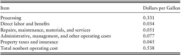
Note: Processing cost represents net processing cost after crediting $0.131/gal. equivalent for the use of stillage powder generated in the plant.
Sources: Wamisho, Ripplinger, and De Laporte (Reference Wamisho, Ripplinger and De Laporte2015), Maung and Gustafson (Reference Maung and Gustafson2011), and Green Vision Group (2014) project documents. Equipment prices were either obtained from the literature or provided by manufacturers through formal quotes.
Capital investment costs (K) comprise engineering and construction costs (e.g., equipment and tank packages, piping and mechanical, steel and enclosures, electrical and instrumentation, engineering, site development, rail, piler and other storage equipment, startup inventories, and other contingencies). Capital costs are calculated ($3.18/gal.) as the present value of the investment costs. Details on capital cost are presented in Table 2. Our investment cost assumes 50% of loan financing of the total investment with a discount rate of 8.25%. To satisfy the smooth-pasting conditions of the equalities, we assume that once the investment is made, an ethanol refinery produces a unit of output per period until abandoned.
Investment Costs, 20 Million Gallon per Year Ethanol Plant

Sources: Wamisho, Ripplinger, and De Laporte (Reference Wamisho, Ripplinger and De Laporte2015), Maung and Gustafson (Reference Maung and Gustafson2011), and Green Vision Group (2014) project documents. Equipment prices were either obtained from the literature or provided by manufacturers through formal quotes.
For our baseline analysis, the value of each sunk cost is calculated as a percentage of the initial capital investment (Schmidt, Luo, and Tauer, Reference Schmit, Luo and Tauer2009). We assume the liquidation/exit cost (l), mothballing (Em ) and reactivation (r) are valued as −25%, 5%, and 10% of initial capital investment, respectively, and the maintenance cost (m) in the mothballed state is valued at 2.5% of K. The baseline sunk costs per gallon of ethanol are as follows: l = $0.795, Em = $0.159, r =$0.318, and m = $0.0795. We assume that mothballing and reactivation costs comprise expenditures on wages and other costs paid in the process of mothballing and reactivation. Preparation costs to sell the plant and clean up the site upon shutting down the refinery permanently are assumed to be negligible and not included in the cost. All costs are assumed to be constant in real terms.
The gross margin of beet ethanol is calculated as the sum of ethanol and beet pulp prices minus the beet price. To compute the gross margin, we convert the sugar beet and beet pulp prices into a dollars per gallon of ethanol equivalent using a conversion rate of 26.5 gallons of ethanol and 0.05 ton of beet pulp produced per ton of energy beets (Maung and Gustafson, Reference Maung and Gustafson2011 ; Wamisho, Ripplinger, and De Laporte, Reference Wamisho, Ripplinger and De Laporte2015). Whereas the stillage powder is credited back into the operating cost, ethanol prices are computed by averaging monthly ethanol prices from January 2000 to December 2014 from the Nebraska Energy Office (2015), representing rack (wholesale) prices (free on board [FOB] price, Omaha, Nebraska). The data for sugar beet prices are obtained from the Farm Financial Database (FINBIN), representing the average value of sugar beets for North Dakota and Minnesota form 2000 to 2014 (FINBIN, 2016). The beet pulp price is from monthly prices representing the Minneapolis market (USDA, 2016).
3.2. Stochastic Gross Margin Parameters
In this section, we estimate the gross margin stochastic parameters. The random variable considered in this study is the ethanol gross margin.
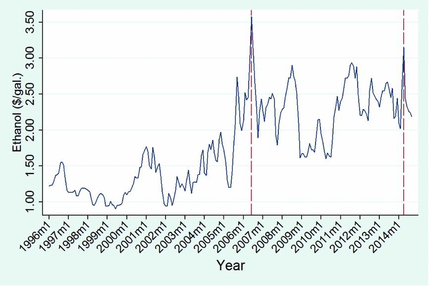
Our data show that ethanol prices were in the range of $1 to $2 per gallon between 2000 and 2004. After 2005, the ethanol price increased steadily, with the exception of a downward blip in 2009 and 2010. The monthly ethanol price peaked in July 2006 at nearly $3.58 per gallon and in April 2014 at $3.15 per gallon. In order to investigate the impact of increasing price volatility starting in late 2006 (see Figure 1), we split the sample into two periods: the full sample period from January 2000 to December 2014 and the subsample period from August 2006 to December 2014. The drift and volatility parameters for these subsample periods are calculated.
Historical Monthly Ethanol Rack Price at Omaha, Nebraska
The gross margins are deflated into real terms using the urban consumer price index (U.S. Department of Labor, 2010). An augmented Dickey-Fuller (ADF) test is applied to determine if the evolution of gross margins follows a random walk or has a unit root. The ADF unit root test results (Table 3) show that we cannot reject the null hypothesis that log of gross margin (ln P) exhibits a unit root at the 99% and 95% confidence level.
Augmented Dickey-Fuller Test for Unit Root
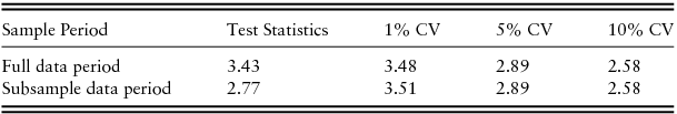
Notes: Full sample period represents data from January 2000 to December 2014, and subsample period is from August 2006 to December 2014. CV represents critical value.
Choosing the appropriate stochastic process for modeling commodity prices should also be based on theoretical consideration in addition to the statistical test results (Dixit and Pindyck, Reference Dixit and Pindyck1994). In addition, Schmit, Luo, and Tauer (Reference Schmit, Luo and Tauer2009), Schmit, Luo, and Conrad (Reference Schmit, Luo and Conrad2011), and Gonzalez, Karali, and Wetzstein et al. (Reference Gonzalez, Karali and Wetzstein2012) found no evidence of mean reversion in U.S. ethanol prices. These authors argue that ethanol price is better modeled using GBM than mean reversion. As such, Postali and Pichcetti (Reference Postali and Pichcetti2006) show that crude oil prices reasonably follow GBM and are strongly correlated with ethanol prices. In fact, Dixit and Pindyck (Reference Dixit and Pindyck1994) argue that commodity prices are shown to exhibit GBM and typically require many years of data to determine with any degree of confidence whether a variable certainly follows mean reversion. Given the ADF test result and having shorter sample data periods, the stochastic variables used in our real option analysis are assumed to evolve according to GBM. Hence, we assume that the gross margin of ethanol evolves exogenously over time through GBM as in equation (1), which is the continuous-time formulation of the random walk. As a result, ln P follows a Brownian motion with drift parameter $\mu = \beta - \frac{1}{2}{\sigma ^2}$
and volatility σ. The total derivative of ln P is the following:
$\mu = \beta - \frac{1}{2}{\sigma ^2}$
and volatility σ. The total derivative of ln P is the following:
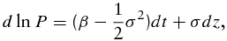 $$\begin{equation}
d\ln P = (\beta - \frac{1}{2}{\sigma ^2})dt + \sigma dz,
\end{equation}$$
$$\begin{equation}
d\ln P = (\beta - \frac{1}{2}{\sigma ^2})dt + \sigma dz,
\end{equation}$$
where P is the gross margin and β contains the parameters to be estimated. GBM requires d ln P to have a unit root, and our resulting series are nonstationary. To remedy this problem, the drift and volatility parameters are computed as the sample mean and standard deviation of the first difference of the natural log of the annual gross margin series. Note that in some months the gross margins are less than zero. To avoid negative values, we vertically scaled up the gross margins by $0.14/gal. for all data points before we ran the regression.Footnote 2 We recovered stochastic parameters displayed in Table 4 using ordinary least squares by regressing Δ ln P on an intercept term and lagged values Δ ln Pt – 1.
Regression Results and Parameters of Gross Margins
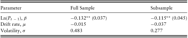
Notes: Standard errors in parentheses. Plus sign indicates significance at the 0.10 level. Asterisks (*, **, and ***) indicate significance at the 0.05, 0.01, and 0.001 level, respectively.
Because the investment analysis is based on annual production, the baseline solutions of real options trigger gross margins are calculated after converting monthly parameters to annual equivalents assuming that both the drift rate and variance of the increments of a Brownian motion are linear in time. For the full data period model, January 2000 to December 2014, the annual drift and volatility parameters are −0.015 and 0.483, respectively, and for the subsample period of August 2006 to December 2014, these parameters are −0.037 and 0.277, respectively (Table 4). The gross margin volatility parameters evolve directly from the root-mean-square error estimation results. Although correlation among all cost and revenue variables certainly determines investment behavior relative to entry and exit decisions, the lack of stochastic data specifically on beet ethanol investment cost and other operating costs do not allow us to capture correlated uncertainty in empirical specification. Therefore, we assume that the magnitude of other operating, investment, mothballing, and reactivation costs are constant, not stochastic.
4. Results and Discussion
The empirical results are presented in two distinct sections. Section 4.1 discusses the results from the baseline solution, along with a comparison of the baseline results with those from the Marshallian approach. Section 4.2 contains results from comparative static and sensitivity analysis to explore how the gross margin trigger value varies with a change in stochastic parameters and underlying investment variables. To conduct the comparative static analysis, we ran a sensitivity analysis to explore the effects of a change in volatility parameters. In addition, we considered how a change in liquidation and reactivation costs could potentially affect the exit and entry decisions for a given level of stochastic parameters.
The Marshallian/NPV entry gross margin is calculated using Wh = ω + δK, where the right-hand side of the equation is the annualized full cost of making and operating the investment. Conversely, the exit gross margin is computed as Wl = ω − δK. Thus, the full cost ω + δK serves as the entry trigger, and the nonbeet operating cost ω as the exit trigger gross margin threshold for making an investment decision. This is the standard Marshallian theory of the long run versus the short run, based on the gap between the full and variable costs (Dixit and Pindyck, Reference Dixit and Pindyck1994). Under the Marshallian approach, at gross margins between Wh and Wl , an idle firm does not invest and an active firm does not exit. However, the firm will abandon the project if the gross margin of ethanol is less than the nonbeet operating cost.
4.1. Baseline Results
Using the parameters from the two sample periods, the real options trigger gross margins are calculated with and without mothballing and reactivation options.Footnote 3 Table 5 presents the calculated baseline trigger gross margins under real options and the Marshallian approach.
Baseline Real Options Trigger Gross Margins, Dollars per Gallon
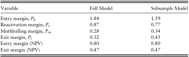
Notes: With managerial flexibility implies entry and exit with mothballing and reactivation options, whereas without managerial flexibility (i.e., inflexible option) represents entry and exit without mothballing and reactivation options. The empirical results show that having the managerial flexibility of mothballing and reactivation does not change the trigger entry and exit gross margins. NPV, net present value.
Using the full sample data, the baseline real options entry gross margin estimate is $1.84/gal., approximately 57% higher than the corresponding Marshallian gross margin of $0.80/gal, and the real options exit gross margin is $0.32/gal., 19% smaller than the Marshallian exit price of $0.47/gal. The inaction gap, between the real options entry and exit gross margins, is $1.53/gal., which is significantly higher than the corresponding entry and exit gap under the Marshallian approach, $0.33/gal. This is an indication that hysteresis is significant and the optimal thresholds with rational expectations of ROA are spread farther apart than the Marshallian ones with static expectations of NPV. The NPV-based gross margins range between $0.8/gal. and $0.47/gal. In this range, an idle firm does not invest and an active firm does not exit. On the exit side, the trigger exit gross margin is $0.47/gal., which is just below the net nonbeet operating cost of $0.54/gal., an indication that once the investment is made, the firm will not abandon the project unless the exit gross margin is sufficiently far less than the net operating cost.
A further real options analysis using the subsample data period, 2006–2014, shows that the inaction gap between the real options entry and exit margin is $1.53/gal., which is smaller than under the full sample data (Table 5). Using the subsample period, the ROA entry threshold margin is found to be $0.25/gal. less than the value obtained under the full sample period. The exit threshold margin also increases $0.13/gal., indicating that as future uncertainty decreases so does the firm's inaction gap.
The drift rate is a trend rate of growth in the gross margins of ethanol, and a positive and increasing drift rate is expected to improve the profitability of the ethanol investment. However, drift rate values in our study are negative in both sample periods, indicating that, in the long-run, there is a potential decline in ethanol gross margins. As depicted in Table 4, volatility parameters in our subsample period are smaller than that in the full sample period. The difference in these parameter values has implications for the threshold behavior of the firm. Given our negative drift rates and comparing the two baseline solutions in Table 5, an idle ethanol firm waits longer to invest and requires a higher threshold gross margin as the volatility of gross margins increases, whereas an active firm is more reluctant to exit the ethanol market once invested. In the next section, we explore in detail how trigger gross margins change for different values of volatility parameters.
We found that mothballing trigger gross margins were $0.28/gal. and $0.34/gal., relatively less than the exit gross margins of $0.32/gal. and $0.45/gal., indicating that the owner of the biorefinery prefers to exit directly, rather than mothballing. This makes sense given that a mothballed state requires the firm to incur additional maintenance costs to keep the plant ready for future reactivation. For mothballing to be an optimal strategy, the trigger mothballing gross margin must be greater than the exit margin (Dixit and Pindyck, Reference Dixit and Pindyck1994). In addition, the model results show that to switch from a mothballed to an active state, the gross margin of ethanol must be $0.871/gal. or $0.77/gal., in the sample and subsample, respectively.
4.2. Competitiveness of Energy Beet–Based Ethanol
One way to evaluate the competitiveness of energy beet ethanol relative to conventional corn ethanol is to compare real options and Marshallian gross margin results from our model to the actual monthly gross margins of corn ethanol. An illustration of historical corn ethanol gross margins is overlaid onto the real options and Marshallian trigger gross margins we find in this study (Figures 2 and 3). These figures provide an intuitive way to compare estimated real options entry and exit gross margins with historical corn ethanol gross margins. In addition, the beet ethanol margins are also calculated based on historical beet and corn ethanol prices and overlaid along with corn ethanol gross margins (Figures 2 and 3). Although energy beet ethanol has not yet been produced, studying potential beet ethanol gross margins illustrates how future beet ethanol gross margins could change, should beet and ethanol stochastic prices follow past price evolution processes.
Real Options (RO) and Net Present Value (NPV) Entry and Exit Trigger Gross Margins Overlaid by Historical Corn and Beet Ethanol Gross Margins, Using the Full Sample Data (note: the horizontal lines represent the RO and NPV entry and exit trigger gross margins calculated as baseline solutions using the full sample data period [see Table 4]; the vertical lines inside Figure 2 are drawn on June 2006, August 2008, and April 2014)

Real Options (RO) and Net Present Value (NPV) Entry and Exit Trigger Gross Margins Overlaid by Historical Corn and Beet Ethanol Gross Margins, Using the Subsample Data (note: the horizontal lines represent the RO entry and exit trigger gross margins, $1.59/gal. and $0.45/gal., respectively, calculated as baseline solutions using subsample data period [see Table 4]; the three vertical lines inside Figure 3 are drawn on June 2006, August 2008, and April 2014)

Our baseline real options entry gross margin is above the historical actual gross margin of corn and beet ethanol for only a small period, an indication that there were few time periods that would have supported beet ethanol plant investment (Figure 2). We counted the number of months in which the real options trigger gross margin is less than that of historical ethanol gross margins. Out of the 180 months studied, there are only 7 months (time periods) that the real option entry trigger gross margin ($1.84/gal.) is less than that of actual corn ethanol gross margins. These 7 months occur after the year 2005, the time period in which the ethanol price was above $2/gal. The number of time periods rose to 11 when we compared with energy beet ethanol gross margins. However, the Marshallian NPV entry trigger margin ($0.8/gal.) would have signaled investments in energy beet ethanol in many time periods given that its value is greater than that of ethanol gross margins. On the exit side, there were quite a number of time periods that would have supported a plant exit.
For further examination into the competitiveness of beet ethanol investments, we again chose past gross margin regimes that represent time periods in which a number of new corn ethanol plants entered the U.S. ethanol market. Figure 3 depicts the later periods of gross margins and the baseline real options trigger margins obtained under the subsample period. The gross margins of the corn and beet ethanol tend to follow similar upward and downward trends. However, as is apparent at times, the gross margins across a few time periods diverge from each other, an indication of the differences in corn and beet feedstock prices. Figure 3 again illustrates that there are few time periods that signal investments in energy beet ethanol.
It is apparent that narrower gross margins could potentially tighten plant profitability, and, in the long run, this condition decreases the value of the ethanol plant. In addition, the biorefinery owner will abandon at a higher threshold exit price because the plant will lose more money when gross margins tighten. As such, the expected flow of profit from, and hence the option value of, the plant falls as the beet ethanol gross margin decreases, implying that higher ethanol prices and/or lower beet prices are required before the firm is willing to invest. Moreover, higher operating costs reduce the value of operating an ethanol refinery, raise the trigger reactivation prices at which a mothballed plant could be reactivated, and raise the mothballing and reactivation price thresholds.
4.3. Effects of Ethanol Gross Margin Volatility
In this section, we present the results from the sensitivity analysis by taking different volatility parameters of ethanol gross margins using a full sample data period. The sensitivity analysis examines 5% incremental increases in the volatility of gross margins from 10% to 60%, keeping β, the discount rate parameter, and sunk and other unit net operating costs constant. Figure 4 shows how trigger gross margins evolve with a change in ethanol gross margin volatility. The vertical line inside Figure 3 is drawn onto the baseline volatility, σ = 0.48, and the corresponding real options trigger gross margins. If there is relatively insignificant uncertainty over the future gross margin of ethanol, σ = 0.1, the trigger entry and exit gross margin will be $1.56/gal. and $0.59/gal., respectively. With a modest change in volatility, for example, a change from 0.1 to 0.15, the zone of inaction (i.e., the distance between the entry and exit trigger gross margins) increases from $0.98/gal. to $1.1/gal., implying that even a small increase in uncertainty affects trigger gross margins.
Real Options Trigger Gross Margins Relative to Changes in Volatility of Ethanol Gross Margins, Using Full Sample Data Parameters
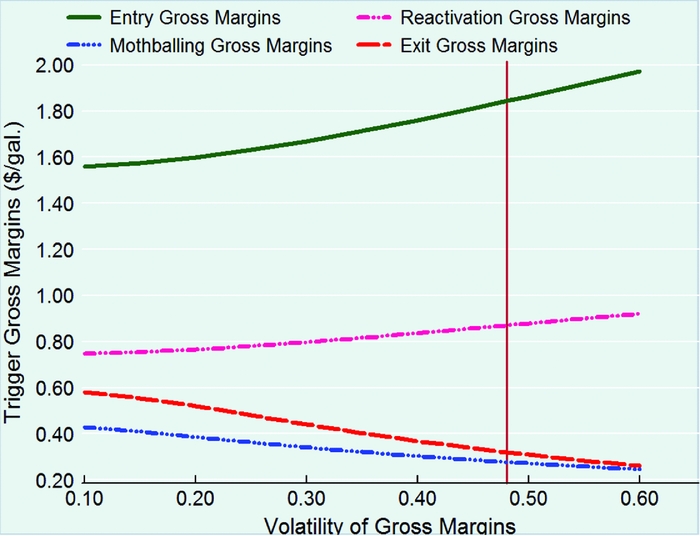
The zone of inaction widens substantially to $1.71/gal. for larger values of σ (= 0.60). The gap between entry and exit gross margins increases as the volatility parameter increases, indicating that hysteresis remains significant even for small changes in ethanol gross margin volatility. Overall, as the volatility of gross margins increases, beet ethanol firms prefer waiting longer to invest. However, once an investment is made, managers in the active state prefer to wait longer before shutting down even if margins are falling. In addition, an increase in gross margin volatility increases the trigger reactivation gross margins in which a mothballed plant is reactivated.
On the mothballing side, at relatively low levels of uncertainty, mothballing trigger gross margins are less than the corresponding exit margins, and the gap between both margins (the range of inactivity) is large. However, mothballing trigger gross margins subsequently start to converge to the exit margins, just passing the baseline value of volatility (Figure 4). With the range of volatility parameters we use, the probability of a sufficiently large increase in gross margins of ethanol is too small to make mothballing economical and a plant will be better off exiting and avoiding the maintenance costs associated with a mothballed state. For mothballing to be an optimal strategy, the trigger real options mothballing gross margin must be greater than the exit margin (Dixit and Pindyck, Reference Dixit and Pindyck1994).
In general, our results show that relatively stable gross margins induce trigger entry gross margins to fall. Once the investment is made, the firm is more willing to stay operating despite there being adverse gross margins temporarily.
4.4. Effects of Liquidation and Reactivation Costs
We further ran sensitivity analysis to explore the effects of liquidation and reactivation costs on trigger gross margins. Liquidation and reactivation costs are simulated in 5% increments and decrements from baseline values. The two panels in Figure 5 show how trigger gross margins evolve with a change in liquidation and reactivation costs based on the full and subsample data sets. Our empirical results from a full sample period show that entry and exit trigger gross margins are around $1.99/gal. and $0.27/gal., respectively, if an active firm is not able to recoup any of the capital investment (i.e., zero liquidation cost upon exiting ethanol market). However, these trigger gross margins are $1.62/gal. and $0.39/gal., respectively, when the liquidation cost is 50% of K. For exposition, if the liquidation cost is zero, the trigger entry and exit gross margins are $1.7/gal. and $0.39/gal., respectively, using the subsample data period. As Figure 5 illustrates, the real options entry trigger gross margins in the subsample period are less than the corresponding entry margins in the full sample period, whereas exit trigger gross margins are otherwise for all values of liquidation used in our sensitivity analysis. As such, the variation in trigger margins between the two data periods is as a result of differences in the volatility parameter. These results assert that, if an active firm foresees that it is able to recover more of its initial capital investment, it is willing to invest at relatively lower gross margins, but at the same time, more quickly prefer the exit option.
Real Options Entry and Exit Trigger Prices Relative to Changes in Liquidation Costs

The empirical results show that trigger mothballing and reactivation gross margins do not change with a change in liquidation costs. However, as shown in the left panel of Figure 5, mothballing is part of the firm's optimal strategy if liquidation costs are close to zero. For liquidation values greater than $0.16/gal., it is optimal for the plant owner to exit directly, thereby recouping some amount of the initial capital, rather than switching to a mothballed state. Therefore, the $0.16/gal. liquidation cost, where these two trigger margins converge, defines the boundary of the liquidation cost space where mothballing ceases to be relevant. Although mothballing is part of the optimal strategy, it only makes sense if the maintenance costs at the mothballed state are less than the net actual operating costs of the ethanol refinery and if the reactivation cost is less than the cost of fresh investment (Dixit and Pindyck, Reference Dixit and Pindyck1994).
With regard to reactivation gross margins, margins are not changed at all for each change in liquidation costs as depicted in Figure 6. Our results show that firms mothball active plants less readily.
Real Options Entry and Exit Trigger Prices Relative to Changes in Reactivation Cost

To this end, mothballing is not an optimal strategy in almost all of the sensitivity analysis because mothballing is useful only if there is a reasonable probability of a substantial increase in revenue in the near future. The real options trigger reactivation gross margins increase with an increase in reactivation costs, implying that firms will reactivate a mothballed plant more readily if the reactivation cost is smaller.
5. Conclusions and Implications of the Findings
This study explores how the decision to invest in a new energy beet ethanol refinery could be affected by ethanol and beet market price uncertainties and underlying irreversible investments. We analyze the optimal rules for exercising the option to invest, mothball, and exit in terms of underlying ethanol and beet price volatility and sunk costs associated with each state of the refinery.
The empirical results show that higher ethanol gross margin volatility causes firms to wait longer before entering and, once active, wait longer before exiting. Hysteresis (inaction) between entry and exit increases with higher levels of ethanol gross margin uncertainty, implying that investment in a new refinery is made more reluctantly, but once made, abandonment is not exercised easily. Under higher levels of gross margin volatility, an active firm waits longer to mothball, and a mothballed firm waits longer to reactivate. Moreover, the expected value of the ethanol biorefinery falls sharply as gross margins shrink, indicating that higher gross margins are required before the firm is willing to invest, and the firm abandons the plant at a higher threshold exit price. With the exception of liquidation costs, trigger gross margins do not rise and fall by very large values with changes in sunk and reactivation costs, suggesting that investment is highly sensitive to volatility in the market gross margin of ethanol and beets, irrespective of owners’ risk preferences and irrespective of the extent to which the riskiness of the project value is correlated with the market. The sensitivity analysis shows that volatility in gross margins of ethanol has much greater effects on exit and entry trigger gross margins and ethanol plant values than investment costs. Empirical results indicate that uncertainty about ethanol prices, beet prices, and sunk costs are important determinants of energy beet investment behavior. We observe that all of the real options trigger margins are quite sensitive to gross margin volatility.
In general, our empirical results demonstrate that the prospect of beet ethanol plant entry into U.S. ethanol markets, and being competitive with conventional corn ethanol, seems uncertain given that the trigger entry gross margins we computed are significantly higher than the gross margins of conventional ethanol. Given the outlook of the current ethanol market situation, uncertainty about beet feedstock costs, coupled with volatility in ethanol prices and higher plant investment costs, poses a significant barrier to investment in energy beet ethanol plants of the scale examined here.
As such, our model results imply that the emergence of energy beet ethanol is unlikely considering the current ethanol market conditions, in part because of strong competition from conventional ethanol and costly beet feedstock. Albeit, one way to make beet ethanol more attractive to investors is through government subsidies. Historical rapid growth in the U.S. ethanol industry has been driven by various incentives and mandates placed on biofuel industries (Babcock, Marette and Tréguer, 2010; Epplin et al., Reference Epplin, Clark, Roberts and Hwang2007; Wetzstein, Reference Wetzstein2010). For example, Schmit, Luo, and Conrad (Reference Schmit, Luo and Conrad2011) found that in the absence of ethanol policies, much of the recent expansionary period would not have existed, and some plant closures would have been imminent given the past market conditions. Yi, Lin, and Thome (Reference Yi, Lin and Thome2015) found that the RFS is a critically important policy for supporting the sustainability of corn-based fuel ethanol production, and that investment and entry subsidies are more effective than production subsidies. As in the United States, ethanol investment decisions in Europe are affected more by government policies and strategic interactions than by economic factors such as ethanol prices, natural gas prices, and feedstock prices (Yi and Lin Lawell, Reference Yi and Lin Lawell2016).
We can argue that the future investment outlook for energy beet ethanol might be more promising and enhanced if ethanol market conditions improve, beet to ethanol conversion technologies become more favorable, and policy interventions in the form of subsidies occur.
Our analysis does not include any federal or state ethanol subsidies or tax incentives, which may change the value of trigger prices. Such policies usually change trigger entry and exit prices by reducing uncertainty and perceived investment risk. From the perspective of beet ethanol investors, the policy uncertainty surrounding the formal designation of beet ethanol as an advanced biofuel is a key factor in investment decision making, in addition to price uncertainty and investment costs. Moreover, obtaining constant beet feedstock supply may be challenging given that energy beet is bulky to transport and its sucrose content quickly deteriorate unless it is transported and processed fairly quickly.
Ethanol from energy beets could play a key role in meeting some of the objectives of the RFS at a time when progress on cellulosic ethanol lags behind proposed schedules and the mandated volumetric requirement under the RFS. Our results may provide a useful tool for potential beet ethanol investors considering investment decisions and for policy makers interested in the development of renewable energy and small-scale industry in rural America.


 Open access