2. Biodiversity drivers and mechanisms

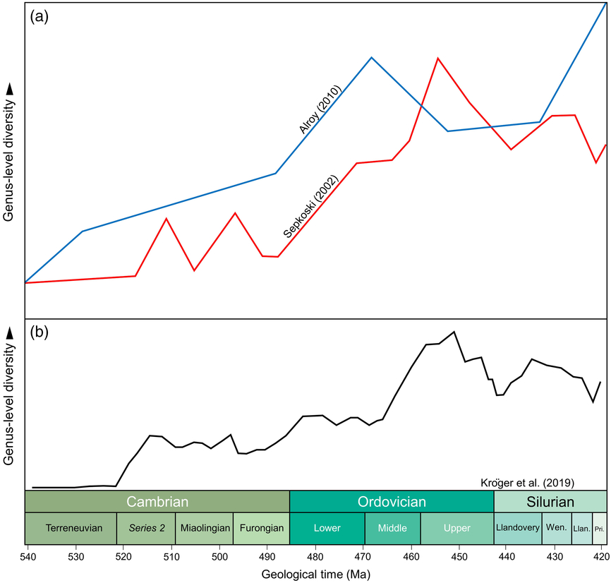
Studies of biodiversity have been focused on taxon counts at various levels, normally families and genera for the abundant invertebrate fossil record and commonly species for the less-rich vertebrate record. Data have been stored in databases, such as the Paleobiology Database (PBDB, e.g. Alroy et al. Reference Alroy, Aberhan, Bottjer, Foote, Fürsich, Harries, Hendy, Holland, Ivany, Kiessling, Kosnik, Marshall, McGowan, Miller, Olszewski, Patzkowsky, Peters, Villier, Wagner, Bonuso, Borkow, Brenneis, Clapham, Fall, Ferguson, Hanson, Krug, Layou, Leckey, Nürnberg, Powers, Sessa, Simpson, Tomašových and Visaggi2008) or the Geobiodiversity Database (GBDB, e.g. Fan et al. Reference Fan, Hou, Chen, Melchin, Goldman, Zhang and Chen2014). The PBDB (initially based on Sepkoski’s compendium: http://strata.geology.wisc.edu/jack/) is most commonly used for global studies of biodiversity through time (https://paleobiodb.org/#/); its data are focused in a number of key regions of the world but are by no means comprehensive. There is now a range of analytical tools available to manage and manipulate data, rather than using raw data (e.g. Sepkoski, Reference Sepkoski1997, Reference Sepkoski2002) techniques such as Shareholder Quorum sampling (Alroy, Reference Alroy2010; Na & Kiessling, Reference Na and Kiessling2015) and Capture–Recapture modelling (Rasmussen et al. Reference Rasmussen, Kröger, Nielsen and Colmenar2019) to provide forms of standardization. For the reasons noted above, data in PBDB or GBDB (the latter being initially focused on extensive Chinese data) are far from complete, but have been proving robust for analyses of palaeobiodiversity and the framing of testable hypotheses. Sepkoski’s compendium and the PBDB show similar trends for the early Palaeozoic biodiversification, displaying a long-term background radiation but indicating different biodiversification pulses (‘peaks’ of biodiversity), depending on the datasets analysed (Fig. 1).

Fig. 1.

Main global patterns by previous authors of genus-level Cambrian–Silurian marine diversity. (a) Comparison of range-based Sepkoski’s (Reference Sepkoski2002) marine diversity patterns with Alroy’s (Reference Alroy2010) sample standardized diversity curve. Adapted from Rasmussen et al. (Reference Rasmussen, Kröger, Nielsen and Colmenar2019, fig. 1). (b) Global curve after Kröger et al. (Reference Kröger, Franeck and Rasmussen2019, fig. 1a) per time genus-level richness.

Geographical isolation has been a key player in the origin and diversification of life. The finches and land tortoises of the Galapagos Islands have served as models for geographic isolation and modification, forming the core of Darwin’s theory of evolution; the theory, based on adaptation, is now well founded and hardened within a well-established framework of heredity. Framed within the context of deep time there is a heterogeneity of diversification across clades, environments, latitudes and regions (see e.g. Harper & Servais, Reference Harper and Servais2013). Stigall (Reference Stigall2018) summarized some of the key drivers associated with the Great Ordovician Biodiversification Event (GOBE) that have been published by a range of authors over the three decades. These include development of islands (whether arcs or microcontinents) during tectonic processes, fluctuating sea levels associated with glaciations, and a heterogeneity of environments from the nearshore to the deep sea and across latitudes, from the poles to the tropics. Both dispersion and vicariance models are complementary with the migration of organisms to new habitats matched by the splitting, by tectonics, of resident populations. Important too, however, is the distinction between alpha, beta and gamma diversity. This concept was applied, principally to brachiopods faunas, during the GOBE (Harper, Reference Harper2010): (1) the expansion of within-community diversity as more niches were created across often heterogeneous environments; (2) sequential development of new communities during the period as biotas occupied deeper-water environments and exploited the many niches available in mudmound and reef build-ups; and (3) the escalation of provincialism during intervals of continental dispersion.

Attempts to identify and verify the (biological or geological) triggers of the individual radiations at a global level have proved challenging, because the curve is the sum of different data from diverse datasets that are all incomplete. Nevertheless, it is important to analyse the peaks of diversity of different fossil groups or fossil categories across different regions. What are the early Palaeozoic biological and geological triggers of these individual radiation(s) and the drivers of the Late Ordovician extinction? Contradictions arise. For example, the GOBE was considered as a rather short event (e.g. Trotter et al. Reference Trotter, Williams, Barnes, Lécuyer and Nicol2008), with indications that massive diversifications took place during a constrained interval associated with rapid cooling; in contrast, the event was originally described as a prolonged, complex biodiversification composed of numerous, diverse radiations (e.g. Sepkoski, Reference Sepkoski, Cooper, Droser and Finney1995; Webby, Reference Webby, Webby, Paris, Droser and Percival2004; see Servais & Harper, Reference Servais and Harper2018 for discussion of the term). Sporadically, more spectacular novel results have sought to explain parts of the radiation in a simple but impactful way; the ‘short event’ was triggered by a single parameter, for example, the GOBE was initiated by a superplume (Barnes, Reference Barnes, Webby, Paris, Droser and Percival2004), an asteroid break-up (Schmitz et al. Reference Schmitz, Harper, Peucker-Ehrenbrink, Stouge, Alwmark, Cronholm, Bergström, Tassinari and Wang2008) or by rapid global cooling during Middle Ordovician time (Rasmussen et al. Reference Rasmussen, Ullmann, Jakobsen, Lindskog, Hansen, Hansen, Eriksson, Dronov, Frei, Korte, Nielsen and Harper2016). On the other hand, an alternative hypothesis that the GOBE is part of a long radiation, with no single, spectacular geological trigger, but probably related to an increase in sea level and the continuous development of large continental shelf areas, has been proposed in lower-profile journals that escape media attention (e.g. Servais et al. Reference Servais, Harper, Li, Munnecke, Owen and Sheehan2009, Reference Servais, Owen, Harper, Kröger and Munnecke2010). In reality, the early Palaeozoic biodiversity curve is overall one of continuous and sustained increase, but with residuals caused partly by sampling bias, both positive and negative, and the waxing and waning of regional biological hotspots or species pumps. All add to a complexity obscured by the process of taxon counting.

3. Key early Palaeozoic biodiversity and extinction events

Palaeontologists have identified a number of discrete diversification and extinction events during the early Palaeozoic Period, each with its own peculiar characteristics. The perception or reality of these events has reinforced the concept that diversity progresses in a series of quantum leaps; by implication, these discrete events are triggered by major environmental shifts, conforming to the Court Jester model. The alternative hypothesis, that the diversification of life is more gradual, is explained by the mutual relationships of groups of evolving organisms, that is, the Red Queen hypothesis. Three diversifications – the Cambrian Explosion, the Great Ordovician Biodiversification Event and the Devonian Nekton Revolution – are apparently partitioned by the Furongian Gap and the Late Ordovician Mass Extinction. Are these in fact discrete diversifications or part of a chain of continuous and gradual diversification?

The Cambrian Explosion is the most profound and visible of the Phanerozoic marine diversifications (and the one attracting the most media attention), and holds the clues for understanding the basic structure of the tree of life and the origin and evolution of animal-based communities. The explosion may extend backwards into the Ediacaran Period, where the Nama biota may represent a recovery after a major extinction, hosting a recognizable metazoan fauna seguing into the explosion proper during early Cambrian time (Darroch et al. Reference Darroch, Smith, LaFlamme and Erwin2018). To date, the evidence is drawn from a number of well-known biotas, related to Fossil-Konservat-Lagerstätten with exceptional preservation, such as the Burgess Shale in the Canadian Rocky Mountains (e.g. Briggs et al. Reference Briggs, Erwin and Collier1994; Erwin & Valentine, Reference Erwin and Valentine2013; Briggs, Reference Briggs2015), Chengjiang in South China (e.g. Hou et al. Reference Hou, Siveter, Siveter, Aldridge, Cong, Gabbott, Ma, Purnell and Williams2017; Yang et al. Reference Yang, Li, Zhu, Condon and Chen2018), Sirius Passet in North Greenland (e.g. Harper et al. Reference Harper, Hammarlund, Topper, Nielsen, Rasmussen, Park and Smith2019a) and others. Among the other key biotas that have been described more recently, the Qingjiang biota from South China (Fu et al. Reference Fu, Tong, Dai, Liu, Yang, Zhang, Cui, Li, Yun, Wu, Sun, Liu, Pei, Gaines and Zhang2019) is the most spectacular, but other discoveries are still to be made. The Cambrian Explosion is distinguished by the apparent origination of bilaterian body plans, essentially phyla, the endemism of its biotas and a dominance in many faunas of predators. The explosion was partitioned by the Sinsk extinction event, at least in Siberian sections (Zhuravlev & Wood, Reference Zhuravlev and Wood2018); prior to the event many stem groups radiated but few survived, while crown group brachiopods and molluscs diversified. A critical part of the ‘explosion’ was the Cambrian substrate revolution (Bottjer et al. Reference Bottjer, Hagadorn and Dornbos2000). Seafloors with microbial mats, so typical of the Ediacaran Period, became increasingly scarce in the shallow-marine environments of Cambrian time, with the evolution of burrowing organisms and vertical bioturbation. The ecological and evolutionary consequences for benthic metazoans were profound, while bioturbation dramatically changed the condition of the substrate in terms of its oxygenation and redox environment (Canfield & Farquhar, Reference Canfield and Farquhar2009). Nevertheless, it is possible that the main pulse of the explosion was fairly short and had virtually concluded prior to the appearance of a more typical Cambrian fossil record (Paterson et al. Reference Paterson, Edgecombe and Lee2019).

The Furongian Biodiversity Gap has been recently noted in a number of papers (e.g. Servais & Harper, Reference Servais and Harper2018) and examined in detail (Harper et al. Reference Harper, Topper, Cascales-Miñana, Servais, Zhang and Ahlberg2019b). There is a marked drop in biodiversity during the Furongian interval. Harper et al. (Reference Harper, Topper, Cascales-Miñana, Servais, Zhang and Ahlberg2019b) have discussed this gap in detail, concluding that diversity has been significantly underestimated by a paucity of examined rock, compounded by a distinctive palaeogeography, extreme climates and fluctuating environments.

The GOBE is the largest marine radiation in the history of life. This extended event, already recognized in the original statistical datasets and introduced as the ‘Ordovician radiations’ by Sepkoski (Reference Sepkoski, Cooper, Droser and Finney1995) and first defined as such by Webby (Reference Webby, Webby, Paris, Droser and Percival2004), covers the entire Ordovician Period and involves biotic radiations at the species, genus and family levels. It is a taxonomic (Sepkoski, Reference Sepkoski, Cooper, Droser and Finney1995), phylogenetic (e.g. Harper et al. Reference Harper, Popov and Holmer2017) and ecological (Droser & Sheehan, Reference Droser and Sheehan1997) event. Sepkoski (Reference Sepkoski, Cooper, Droser and Finney1995) noted that the Ordovician biodiversification consisted of a series of smaller events across the constituent taxonomic groups. Diversity curves for most of the biotic groups were provided in Webby et al. (Reference Webby, Paris, Droser and Percival2004) with discussions of the patterns and trends within each group. It became evident that considerable diacronism across regions and taxonomic groups and the patterns were present in the different datasets. In simple terms the ‘Ordovician Plankton Revolution’ was already accelerating during late Cambrian time, providing a source of nutrients for the filter-feeding and deposit-feeding benthos (Servais et al. Reference Servais, Lehnert, Li, Mullins, Munnecke, Nützel and Vecoli2008) and subsequent rise of metazoan reef systems later during Ordovician time. Harper (Reference Harper2006) summarized the many dimensions of the event and Harper (Reference Harper2010) focused specifically on diversity within the Brachiopoda. Many other aspects of the event have been summarized during the last decade (e.g. Munnecke et al. Reference Munnecke, Calner, Harper and Servais2010; Servais et al. Reference Servais, Owen, Harper, Kröger and Munnecke2010; Harper et al. Reference Harper, Rasmussen, Liljeroth, Blodgett, Candela, Jin, Percival, Rong, Villas, Zhan, Harper and Servais2013; Servais & Harper, Reference Servais and Harper2018).

Significantly, some of the typical (soft body) fossils of the Cambrian Explosion have now also been found in the Fezouata Biota from Lower Ordovician deposits of Morocco (Van Roy et al. Reference Van Roy, Orr, Botting, Muir, Vinther, Lefebvre, El Hariri and Briggs2010; Lefebvre et al. Reference Lefebvre, Gutierrez-Marco, Lehnert, Martin, Nowak, Akodad, Hariri and Servais2018), indicating that faunas typical of the Cambrian Explosion survived after the Furongian Gap and were still present during the GOBE. The Cambrian Explosion seems indeed to be related in part to a taphonomical window (e.g. Butterfield, Reference Butterfield2003; Strang et al. Reference Strang, Armstrong and Harper2016) but under exceptional conditions; the iconic fossils of the Cambrian Explosion might be found later in the fossil record, for example, in Lower Ordovician strata.

A greater granularity and resolution of data in the Paleobiology Database has identified more discrete events against a background of overall diversity increase (Franeck & Liow, Reference Franeck and Liow2019; Kröger et al. Reference Kröger, Franeck and Rasmussen2019; Rasmussen et al. Reference Rasmussen, Kröger, Nielsen and Colmenar2019; Stigall et al. Reference Stigall, Edwards, Freeman and Rasmussen2019). The cascading trend in biodiversity was ascribed to a number of short-term environmental drivers, accumulating diversity most dramatically from early Middle Ordovician time onwards and abruptly curtailed by the end Ordovician, volcanically induced, extinctions (Rasmussen et al. Reference Rasmussen, Kröger, Nielsen and Colmenar2019). Within this general framework, Franeck & Liow (Reference Franeck and Liow2019) considered the Middle Ordovician biodiversity hike was a global phenomenon (based on PBDB data from mainly Baltica and Laurentia); diversifications before and after were more regional. Stigall et al. (Reference Stigall, Edwards, Freeman and Rasmussen2019) have developed an elegant model of coordinated biotic and abiotic change, focused on the Darriwilian Stage of the Middle Ordovician Series. Increasing diversity in many groups is linked to a decrease in ocean temperatures, an increase in oxygen levels and a decrease in pulses of anoxia. These factors are linked to an increase in the complexity and diversity of some elements of the ecosystem, mainly the benthos, accelerated intercontinental dispersal and an increase in body size. The GOBE sensu Stigall et al. (Reference Stigall, Edwards, Freeman and Rasmussen2019) as a whole is partitioned into Pre-GOBE, Main GOBE and Peak GOBE phases. Some of these themes are elaborated by Kröger et al. (Reference Kröger, Franeck and Rasmussen2019) in their demonstration of the resilience of the Ordovician ecosystem; the volatility of the longevity of species (on average 5 Ma in the Cambrian and 10 Ma in the Ordovician) decreases through time.

The Ordovician biodiversifications have been aligned with a number of ecological processes, each capable of generating alpha and beta diversity. The ‘Ordovician Substrate Revolution’ involved the modification of the seafloor by cyanobacterial films, produced by planktic bacteria, over extensive areas of the Middle Ordovician Baltic palaeobasin. These were rapidly mineralized, and the resulting hardgrounds were colonized by various stalked echinoderms, bryozoans and boring animals, while the soft substrate underneath the hardgrounds were occupied by abundant ichnofauna. The formation of hardgrounds on bioherms was more patchy and usually in shallower water. These hardgrounds in turn produced carbonate detritus over large areas of the seafloor around the bioherms. These hardgrounds provided a new focus for the benthos and the availability of more niches associated with carbonate environments and factories (Rozhnov, Reference Rozhnov, Zhang, Zhan, Fan and Muir2017).

The ‘Ordovician Bioerosion Revolution’ was described as a major change during the GOBE, defined as a dramatic diversification of macroboring ichnotaxa during Middle and Late Ordovician time (Wilson & Palmer, Reference Wilson and Palmer2006). The intensity of carbonate substrate bioerosion greatly increased, reaching highest levels during Late Ordovician and early Silurian time. Such important bioerosion was not achieved again until the Jurassic Period. This abundant ichnological diversity was considered by Wilson & Palmer (Reference Wilson and Palmer2006) as directly related to the GOBE, reflecting niche differentiation on hard substrates at that time.

The Late Ordovician Mass Extinction (LOME) was the first of the big five extinctions (Harper et al. Reference Harper, Hammarlund and Rasmussen2014), taxonomically severe, classically presented in two phases but causing only slight disruption to the ecosystem. The first phase was associated with global cooling, and regression restricted on-shelf habitats as the continental shelves were exposed and deep-water biotas suffered as habitats were destroyed by anoxia; during the second phase, cooler-water faunas, such as the Hirnantia brachiopod fauna, began to dominate globally as tropical biotas were largely removed.

During and after the GOBE, parts of the water column were filled with a diversity of planktonic life. However, it was only during the Devonian Nekton Revolution that larger animals moved out of the shadow of the GOBE to participate in events in the water column (Klug et al. Reference Klug, Kröger, Kiessling, Mullins, Servais, Frýda, Korn and Turner2010). Following a clear shift of a number of organisms from the benthos to the plankton near the Cambrian–Ordovician boundary, by late Silurian and Devonian time space on the seabed may have become exhausted; demersal and nekton life modes were initiated by this competition for space and resources on the seafloor, as well as the availability of vacant ecospace and planktonic food.

4. Biodiversity in the seas

The taxonomic diversity of the main animal groups has been plotted from data in the PBDB providing granularity for interrogation. Many of the illustrated diversity plots (Figs 2–4) clearly demonstrate that for many groups the data in the PBDB are not complete, and that studies published separately by specialists of the individual fossil groups usually provide much more precise data. The present study is therefore at best a short review of data, and the reader is referred to more detailed diversity studies in the extensive specialist literature of the different fossil groups, which remain essential for a full understanding of the taxonomy, biostratigraphical control and palaeoecological signal of each group.

Fig. 2.

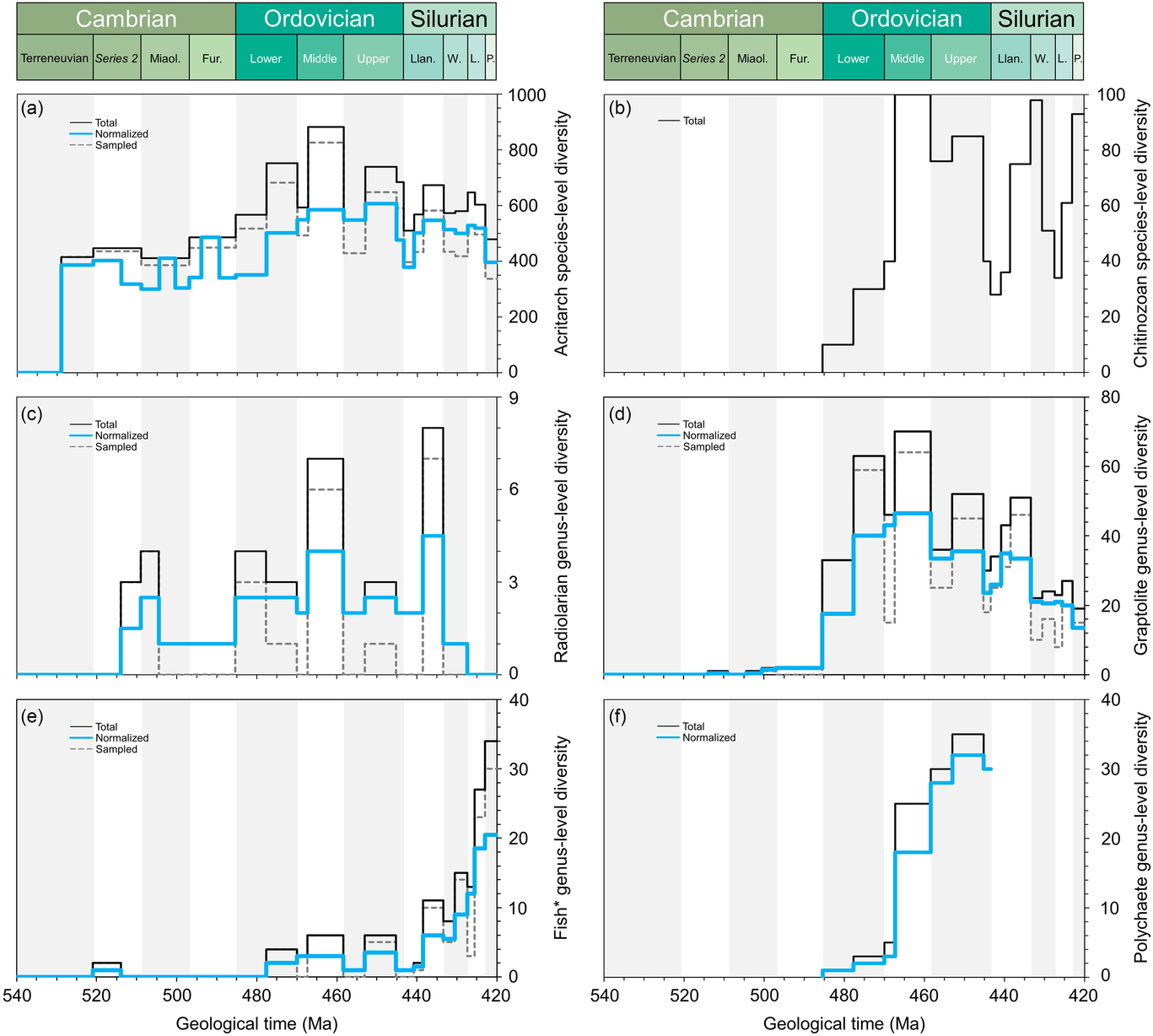
Comparative plots of Cambrian–Silurian genus-level (and species-level for acritarchs) marine diversity patterns by biological groups (I): (a) Acritarcha, (b) Chitinozoa, (c) Radiolaria, (d) Graptolithina, (e) Fishes (i.e. Agnatha, Hyperotreti, Pteraspidomorphi, Thelodonti, Anaspida, Galeaspida, Osteostraci, Chondrichthyes, Acanthodii, Osteichthyes) and (f) Polychaeta. Except for chitinozoan and polychaete patterns, the total, normalized and sampled diversity is plotted. See methods in Section 4 for details.

Fig. 3.

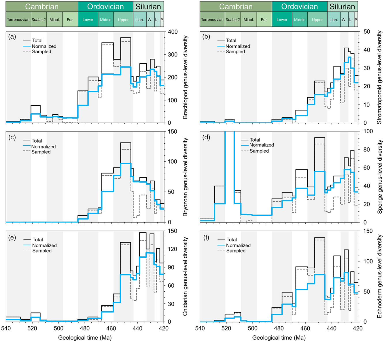
Comparative plots of Cambrian–Silurian genus-level marine diversity patterns by biological groups (II): (a) Brachiopoda, (b) Stromatoporoidea, (c) Bryozoa, (d) Porifera, (e) Cnidaria and (f) Echinodermata. In all cases, the total, normalized and sampled diversity is plotted. See methods in Section 4 for details.

Fig. 4.

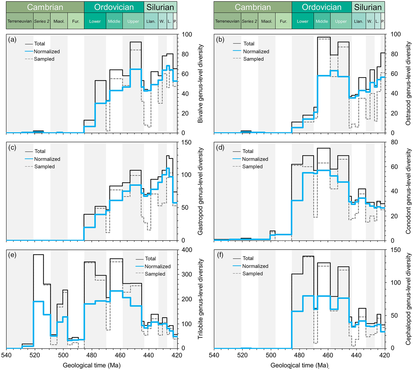
Comparative plots of Cambrian–Silurian genus-level marine diversity patterns by biological groups (III): (a) Bivalvia, (b) Ostracoda, (c) Gastropoda, (d) Conodonta, (e) Trilobita and (f) Cephalopoda. In all cases, the total, normalized and sampled diversity is plotted. See methods in Section 4 for details.

In order to explore the main diversity dynamics in the marine realm, the tool ‘Diversity over time’ in the Paleobiology Database (https://paleobiodb.org/classic/displayDownloadGenerator) has been used to download raw diversity counts of most of the main groups considered here (Figs 2–4). The downloads were performed on 21 February 2019 and involved 14 marine groups (in alphabetical order): Bivalvia, Brachiopoda, Bryozoa, Cephalopoda, Cnidaria, Conodonta, Echinodermata, Gastropoda, Graptolithina, Ostracoda, Porifera, Radiolaria, Stromatoporoidea and Trilobita. Total marine diversity counts were also investigated. The diversity data of ‘fishes’ (Fig. 2e), involving the Agnatha, Hyperotreti, Pteraspidomorphi, Thelodonti, Anaspida, Galeaspida, Osteostraci, Chondrichthyes, Acanthodii and Osteichthyes were treated separately as a combined total (downloaded on 15 March 2019). In all cases, diversity counts were restricted to the Cambrian–Silurian interval. Data were downloaded at the genus level, and only named taxa are considered in the datasets used here. Uncertain genus and species occurrences were excluded, and it is assumed that extant taxa range through to present. The rest of the parameters were considered, following default options. Moreover, due to inherent PBDB limitations on certain groups, some diversity data were directly adapted from review papers. Ordovician polychaete diversity patterns are from Eriksson et al. (Reference Eriksson, Hints, Paxton and Tonarova2013), whereas the Ordovician chitinozoan diversity curve is adapted from Achab & Paris (Reference Achab and Paris2007). The early Palaeozoic data on the phytoplankton (acritarchs) is based on unpublished data (D Kroeck, pers. comm, 2019).

Figures 2–4 include the total diversity (i.e. all taxa observed in a given time interval), the sampled diversity (i.e. all taxa recovered in a given time interval) and normalized diversity sensu Cooper (Reference Cooper, Webby, Paris, Droser and Percival2004) (i.e. all taxa ranging from the interval below to the interval above, plus half the taxa that originate and/or become extinct within the interval, plus half of single-interval taxa).

Evidence suggests that while the Ediacara biota is dominated by lower-grade metazoans such as rangeomorphs and possibly sponges and cnidarians, the early Palaeozoic diversifications are based on the emergence of the bilaterians: the ecdysozoans, lophophorates and the deuterostomes. The phyto- and zooplankton groups have first Cambrian records and expand during the Ordovician Period as the base of the trophic chain broadened. The lophophorates (brachiopods, bryozoans and molluscs) have contrasting stratigraphical distributions, as do the ecdysozoans (arthropod and related groups) and the deuterostomes (echinoderms and hemichordates).

In global datasets, a major ecological shift occurred between the Cambrian and Ordovician periods (Klug et al. Reference Klug, Kröger, Kiessling, Mullins, Servais, Frýda, Korn and Turner2010) with the substantial appearance of planktonic groups; this shift had clearly started during late Cambrian time (Servais et al. Reference Servais, Perrier, Danelian, Klug, Martin, Munnecke, Nowak, Nützel, Vandenbroucke, Williams and Rasmussen2016). The fossil record of the smaller fractions of the plankton (bacterio- and picoplankton) is unknown, and that of the microphytoplankton is only partly known. The PBDB does not include any data on these important groups at the base of the marine food web. The diversity of the organic-walled microphytoplankton has been studied, partly in detail (e.g. Nowak et al. Reference Nowak, Servais, Monnet, Molyneux and Vandenbroucke2015), but these data are not yet included in the PBDB. The presence of calcareous microplankton during the early Palaeozoic Era is still under debate (e.g. Munnecke & Servais, Reference Munnecke and Servais2008) and siliceous phytoplankton is unknown. The organic-walled fraction of the phytoplankton is represented by the acritarchs, showing a continuous increase between the early Cambrian and Late Ordovician periods (Fig. 2a). Some studies show a strong increase in diversity during Furongian time (Nowak et al. Reference Nowak, Servais, Monnet, Molyneux and Vandenbroucke2015), indicating the onset of the Ordovician plankton revolution (Servais et al. Reference Servais, Perrier, Danelian, Klug, Martin, Munnecke, Nowak, Nützel, Vandenbroucke, Williams and Rasmussen2016). The diversity of the acritarch microphytoplankton increases up through the upper Cambrian strata, but is observed to decrease in the Katian deposits.

The most extensively studied zooplanktonic group is the graptolites. Graptolite evolution during early Palaeozoic time has been discussed in detail (e.g. Maletz, Reference Maletz2017). Members of the fixed, benthic dendroids detached in the latest Cambrian to join the plankton, developing life-modes as automobile sweep-net feeders; their stipe configurations and thecal form became adapted to this life mode, with colony shapes aiding mobility and the harvesting of food. These morphological changes are tracked through a succession of evolutionary faunas, the anisograptid, dichograptid, diplograptid and monograptid assemblages. Graptolite biodiversity peaked during Late Ordovician time, suffered significantly at the end of the Ordovician Period and recovered during early Silurian time (Fig. 2d) with the radiation of the monograptids. Compared with the PBDB, the more detailed study of the diversification of the graptolites by Crampton et al. (Reference Crampton, Cooper, Sadler and Foote2016) indicates a first appearance of planktonic forms in the basal Tremadocian and the most important diversity increase during the middle Floian Age.

The other zooplanktonic groups with a sufficiently documented, but still incomplete, fossil record are the radiolarians and the chitinozoans. Radiolarians have only been sporadically studied, with few occurrences in the Cambrian System and a more complete record in the Ordovician System (Fig. 2c), but the datasets are still fairly poorly populated. Chitinozoans, similar to the graptolites, make their first appearance in the basal Ordovician strata. The global diversity is driven by the aggregation of regional trends reaching highest levels in the lower Katian Stage (Fig. 2b).

The fixed benthos is dominated by suspension-feeding organisms. The brachiopods dominated the Palaeozoic benthos, appearing in significant numbers during the Cambrian Explosion, and established a wide range of lifestyles supplemented during the GOBE (Topper et al. Reference Topper, Zhifei, Gutierrez-Marco and Harper2018). Cambrian brachiopod faunas are generally of low diversity (Fig. 3a), dominated by nonarticulates together with billingsellides, chileids, obolellides, naukatides, orthides and pentamerides with protorthides featuring sporadically. Nevertheless, the majority of brachiopod life modes had already been established by early Cambrian time with few additions later during the Ordovician Period (Topper et al. Reference Topper, Zhifei, Gutierrez-Marco and Harper2018). The Early Ordovician diversifications around parts of tropical Gondwana (e.g. Zhan & Harper, 1996) escalated during Middle Ordovician time (Fig. 3a) on Baltica and Laurentia, associated with cooler-water conditions and the delivery of nutrients onto shelves by vigorous oceanic circulation (Rasmussen et al. Reference Rasmussen, Ullmann, Jakobsen, Lindskog, Hansen, Hansen, Eriksson, Dronov, Frei, Korte, Nielsen and Harper2016) segueing into the diverse later Ordovician brachiopod fauna associated with carbonate factories (Harper & Rong, Reference Harper and Rong2001). A number of adaptations can be mapped onto the diversification, for example the dominance of recumbent lifestyles among the strophomenides and the development of cyrtomatodont dentition and brachidia in the spire-bearing forms, and many diversifications are coincident with the Ordovician substrate revolution.

The bryozoans were represented by the trepostome Stenolaemata, forming part of the low-level benthos and commonly participating in reefal structures as bush-like colonies with polygonal apertures. The first skeletalized bryozoans were present during Tremadocian time, but markedly diversified during the Ordovician Period (Fig. 3c), reaching a peak during the Katian Age (Ernst, Reference Ernst2018).

Polychaetes were prominent benthic predators in early Palaeozoic ecosystems, apparently originating during Early Ordovician time, diversifying through the period to peak in the Katian Age (Fig. 2f). Data from the Cambrian Period are sparse and a Silurian diversity curve has yet to be drawn. The data presented here are limited to the Ordovician Period and based on Eriksson et al. (Reference Eriksson, Hints, Paxton and Tonarova2013), indicating a significant Middle Ordovician radiation related to the substantial number of studies from Baltica.

The cnidarians, represented mainly by the rugose and tabulate corals, escalated their diversities during Late Ordovician and Silurian time (Fig. 3e) and are commonly associated with shallow-water, carbonate environments and amenable substrates.

The molluscs (bivalves and gastropods) showed a steady increase in diversity during the Ordovician Period (Fig. 4a, c) but in lower numbers than the brachiopods, which became established as the dominant bilaterian benthos throughout most of Palaeozoic time. There are no sudden explosions of taxa; rather each is defined in terms of an individual pattern which combines to form the global signal. Bivalves are reported from the lower Cambrian System, but diversified during Ordovician time to peak during the Katian (Late Ordovician) Age. During the radiation, actinodonts, heterodonts and taxodonts evolved, associated with predominantly deposit- and suspension-feeding life modes. The group suffered a major extinction at the end of Ordovician time, slowly recovering during early Silurian time and stabilizing at low diversities. Gastropods were dominated by deposit feeders and herbivores and exhibit similar diversity trends to those of the bivalves, that is, showing a gradual increase through Ordovician time with losses at the end of the Ordovician Period and a recovery during the Silurian Period.

The cephalopods appeared during late Cambrian time and radiated during Early Ordovician time (Fig. 4f), particularly diverse on the shallow-water tropical and subtropical platforms, probably first as part of the swimming nektobenthos and later moving into the pelagic realm. They have been implicated as predators in an Early Ordovician arms race. The group peaked again during the Katian Age, increasing in size, and again commonly associated with carbonate factories.

Considered to be at or near the top of the marine trophic web, the cephalopods were joined in larger numbers by early vertebrates much later during the Silurian Period. There were a few fishes in the water column (Fig. 2e), but eurypterids may have joined the cephalopods as apex predators.

The mobile nektobenthos is dominated by the trilobites. The pattern is more complex than in other groups (Fig. 4e). The trilobites were the key element of the Cambrian Evolutionary Fauna, with the Olenellina, Ptychopariina and Redlichiina dominating the mobile benthos. The group first peaked shortly after their appearance in Series 2, but suffered a substantial drop, apparent or real, in diversity during the Furongian Epoch. A massive radiation during the Early Ordovician Period introduced a number of new groups with new adaptations: visual systems became more sophisticated and enrolment mechanisms more secure. The Asaphina, Calymenina, Odontopleurida and Trinucleidina diversified while the cyclopygids and telephinids joined the epipelagic and mesopelagic realms, respectively (partially departing from the nektobenthos). Critical was the gradual transition from the Ibex fauna to the Whiterock fauna, the latter originating in more offshore environments but with more intense diversifications in lower latitudes (Adrain et al. Reference Adrain, Fortey and Westrop1998). During Ordovician time the trilobite diversity curve was cumulative, comprising more than one component pattern (Adrain et al. Reference Adrain, Fortey and Westrop1998).

Ostracods were relatively diverse during the Middle and Late Ordovician Period but suffered dramatically during the end Ordovician extinctions (Fig. 4b), recovering gradually during the Silurian Period.

Within the deuterostomes, the echinoderms were presentduring the Cambrian Explosion and accelerated in diversity during the Katian Age through the appearance of diverse stalked forms, the blastoid, crinoid and cystoid faunas, forming part of the higher-level filter-feeding benthos (Fig. 3f). There are a number of more aberrant echinoderms reported from Cambrian Series 2, such as the helioplacoids, which were mud-stickers best adapted to life on lower Cambrian matgrounds. The stalked echinoderms, associated with a firmer seabed (during the first stages of the Ordovician substrate revolution), were of generally low diversity during the Early Ordovician Period but rose to a peak in the Katian Age before dropping at the end of the Ordovician Period; their Katian prominence was recovered during the Llandovery Epoch. The different groups of echinoderms show a very diverse and complex pattern of radiations that can be traced in detail in publications related to these groups (e.g. Sprinkle & Guensburg, Reference Sprinkle, Guensburg, Webby, Paris, Droser and Percival2004).

The conodonts are generally retrieved by acid treatment and are therefore partly reliant on the availability of acid residues from carbonates. They are represented in the Cambrian strata by the protoconodonts, simple cones of unknown precise affinity. Euconodonts are relatively common throughout Ordovician time, but the occurrences of the group dropped during the Silurian Period (Fig. 4d). The euconodonts exhibit marked provincialism during intervals within the Ordovician and Silurian periods, suggesting their dominant life mode was nektobenthic.

The fishes have a moderate early Palaeozoic record, dominated by nektobenthic placoderms during the Ordovician Period. Numbers escalate during the Ludlow and Pridoli epochs (Fig. 2e). The diversity data highlight the occurrence of Haikouichthys and Myllokunmingia from the lower Cambrian Chengjiang Lagerstätte, followed by a gap until the exponential increase in the number of taxa through the low-diversity armoured, jawless, ostracoderm faunas during the Ordovician Period to the appearance of the jawed, acanthodians, chrondrichtheyans and placocoderms during the later Silurian and into the Early Devonian periods when they migrated into the water column and participated in the Nekton Revolution (Klug et al. Reference Klug, Kröger, Kiessling, Mullins, Servais, Frýda, Korn and Turner2010).

Carbonate mudmounds, composed of algal material together with sponge reefs constructed by archaeocythans, are common in lower–middle Cambrian deposits and algal build-ups continued during the Early Ordovician Period (Fig. 3b), seguing into metazoan-dominated reefs with bryozoan and coral reef-builders during the later Ordovician Period. Reef-built ecosystems were dominated by the spongiform archaeocyathans during Series 2, proving a massive diversity hike during early–middle Cambrian time; sponges show a progressive diversification during the Ordovician Period with a peak in the Katian Age, a drop at the end of the Ordovician Period and a recovery during the Silurian Period. During much of the Early Ordovician Period, reef building was restricted to microbial organisms (not captured in the available data); in the later part of the period, a number of further key metazoan players in the GOBE participated in reef building. Stromatoporoids, particularly in carbonate environments, gradually increased in diversity during the Ordovician and Silurian periods to peak in the Wenlock and Ludlow epochs (Fig. 3d). These were joined by corals with increasing numbers of genera from Middle and Upper Ordovician into Silurian time.

The diversity trends of the individual fossil groups (Figs 2–4) clearly indicate different scenarios. The Cambrian Explosion is visible for some groups, but not all. The Furongian Gap is present for many of the groups appearing in the Cambrian Period. The GOBE is clearly the sum of different radiations; the various groups clearly have their ‘major biodiversity pulses’ at different time intervals with different intensities, some during the Early and others during the Middle and Late Ordovician Period.

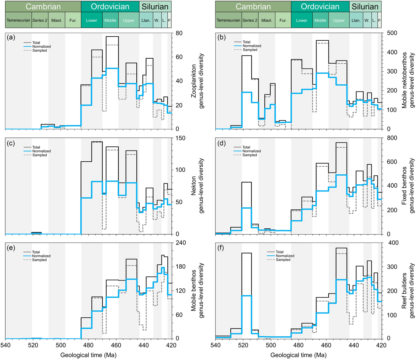
It is particularly interesting to attempt to group the different fossil groups into some major categories (Fig. 5): plankton, mobile nektobenthos, nekton, fixed benthos, mobile benthos and reef builders. Data analysis was performed by taxonomic and ecological groups/categories as follows: zooplankton (graptolites and radiolarians), mobile nektobenthos (i.e. ostracods and trilobites), nekton (i.e. cephalopods and fishes), fixed benthos (i.e. brachiopods, bryozoans, echinoderms, sponges and stromatoporoids), mobile benthos (i.e. bivalves and gastropods) and reef builders (i.e. bryozoans, cnidarians, sponges and stromatoporoids). It is, however, not straightforward to classify an individual fossil group within a single category, because several groups can clearly be categorized in different entities. The cephalopods, for example, had different life modes from nektobenthic to fully nektonic. Some organisms have complex life cycles, with parts of their life cycle being in the plankton and other parts in the benthos. The analyses of the diversity changes of the different categories therefore has to be considered with care. Nevertheless, a few pointers are obvious (Fig. 5). The plankton includes the phytoplankton that increasingly diversified over the entire early Palaeozoic Era, whereas graptolites and chitinozoans only massively arrived during Early Ordovician time (Fig. 5a). The groups attributed to the nekton indicate this dramatic change at the onset of the Ordovician Period, when the water column started to be filled with planktonic/nektonic organisms (Fig. 5c). The mobile nektobenthos (Fig. 5b) and the fixed benthos (Fig. 5d) show peaks of diversity during the Cambrian Explosion and again, after the Furongian Gap, during the GOBE. However, the mobile benthos only shows a clear diversification from Early Ordovician time (Fig. 5e). The reef-building organisms show two clearly distinct ecosystems between the archaeocythan-sponge reefs during early–middle Cambrian time, and bryozoan-sponge-reefs during Middle–Late Ordovician time (Fig. 5f). The different datasets highlight that the GOBE clearly started as early as during Early Ordovician (if not late Cambrian) time and that the Ordovician radiation indicates a three-fold diversification with plankton followed by the benthos and the reef builders (compare Servais & Harper, Reference Servais and Harper2018).

Fig. 5.

Comparative plots of Cambrian–Silurian genus-level marine diversity patterns by simplified ecological categories: (a) zooplankton (graptolites and radiolarians), (b) mobile nektobenthos (i.e. ostracods and trilobites), (c) nekton (i.e. cephalopods and fishes), (d) fixed benthos (i.e. brachiopods, bryozoans, echinoderms, sponges and stromatoporoids), (e) mobile benthos (i.e. bivalves and gastropods) and (f) reef builders (i.e. bryozoans, cnidarians, sponges and stromatoporoids). In all cases, the total, normalized and sampled diversity is plotted. See methods in Section 4 for details.

5. A portfolio of potential triggers

Many publications deal with the triggers of the radiation and diversification ‘pulses’. Such studies focused either on global diversity changes, explaining globally visible radiation or extinction events, or on regional scenarios, explaining events at the scale of a basin or a continental margin. Similarly, several studies focused on detecting the trigger of the radiation of separate fossil groups, locally or globally. At present there is a wide range of publications, partly contradicting each other, with a large portfolio of potential triggers of the individual radiations, biodiversification pulses or extinctions. The causes of the early Palaeozoic events have been classified in terms of extrinsic (abiotic) and intrinsic (biotic) triggers, drivers and enablers, and those explicable by the Court Jester and Red Queen models (e.g. Harper et al. Reference Harper, Zhan and Jin2015 for explanations of the GOBE). Very few triggers can be directly associated with individual radiations and extinctions.

A number of papers have attempted to understand the causes of the Cambrian Explosion. Smith & Harper (Reference Smith and Harper2013) assembled the various drivers and enablers into an inclusive model for the Cambrian Explosion. The model is constructed around the major marine transgression marked by the Great Unconformity on Laurentia and the subsequent erosion of the regolith expelling Ca and PO₄ ions into the oceans and generating biomineralization through cell toxicity, together with increasing nutrient levels. Genome patterning had a key role and bilaterian animals modified the substrates (oxygenating the sediment through bioturbation), developed predator–prey relationships with more complex food webs and moved into the water column. These factors acted in consort to create more habitable areas on the sea floor and in the water column, permitting an explosion of animal diversity.

Similarly, a substantial number of publications and larger, international research projects sponsored by the International Union of Geological Sciences (e.g. Harper et al. Reference Harper, Li, Munnecke, Owen, Servais and Sheehan2011; Harper & Servais, Reference Harper and Servais2013, Reference Harper and Servais2018) were and are focused on the search for triggers of the GOBE. Following the Furongian Gap, diversity apparently picked up pace with the establishment of the GOBE. The causes of this exceptional and prolonged diversification have been discussed in many tens of publications (see Harper et al. Reference Harper, Zhan and Jin2015 for a brief review and tabulation of principal alleged causes). There is a family of intrinsic drivers based on the biological interactions within the ecosystem and possibly explicable by the Red Queen model. The Plankton Revolution (Servais et al. Reference Servais, Lehnert, Li, Mullins, Munnecke, Nützel and Vecoli2008) that had already begun in the late Cambrian Period (Servais et al. Reference Servais, Perrier, Danelian, Klug, Martin, Munnecke, Nowak, Nützel, Vandenbroucke, Williams and Rasmussen2016) fuelled the ecosystem from the base of the food chain. Strong evidence, that is, the presence of large, sweep-net feeders such as the early Cambrian Tamisiocaris (Vinther et al. Reference Vinther, Stein, Longrich and Harper2014) and the Early Ordovician anomalocaridid from Fezouata (Van Roy et al. Reference Van Roy, Daley and Briggs2015), suggests that the water column was already replete with nutrients from the early stages of the evolution of complex animal communities. Intricate food webs containing a range of predators were rapidly established during the early stages of the Cambrian Explosion (Vannier et al. Reference Vannier, Arci, Taylor and Caron2018) and developed through the Ordovician Period. Predator–prey relations escalated during Early Ordovician time with the diversification of the orthoconic nautiloids (Kröger et al. Reference Kröger, Servais and Zhang2009), driving a greater armouring, infaunalization and mobility of prey. In addition, there was increasing competition on the seabed for space and resources, as alpha diversity within communities increased. A large range of enabling factors, extrinsic and mostly explicable by the Court Jester model, provided a favourable milieu and stimuli to help generate biodiversity. Factors such as the asteroid impact Intermediate Disturbance Hypothesis (clearing the seabed for recolonization (Schmitz et al. Reference Schmitz, Harper, Peucker-Ehrenbrink, Stouge, Alwmark, Cronholm, Bergström, Tassinari and Wang2008), the erosion of emergent mountain chains (providing erosional products and nutrients; Miller & Mao, Reference Miller and Mao1995), global cooling (reduction in temperature more compatible with metazoan metabolism and skeletal growth; Achab & Paris, Reference Achab and Paris2007; Trotter et al. Reference Trotter, Williams, Barnes, Lécuyer and Nicol2008), high sea levels (providing increased habitable platform areas; Kiessling et al. Reference Kiessling, Flügel and Golonka2003; Nardin & Lefebvre, Reference Nardin and Lefebvre2010), oxygenation (pulse of atmospheric oxygen aids metabolism, production of collagen and skeletal material; Berner et al. Reference Berner, VandenBrooks and Ward2007; Saltzman et al. Reference Saltzman, Young, Kump, Gill, Lyons and Runnegar2011; C Diamond, unpub. thesis, Ohio State University, 2013), substrate change (general trend from carbonate to siliciclastic substrates favoured particular groups of organisms; Miller & Connolly, Reference Miller and Connolly2001), superplume activity (providing nutrients; Barnes, Reference Barnes, Webby, Paris, Droser and Percival2004), tectonic and magmatic activity (creation of island habitats, providing intra-oceanic nurseries, museums and stepping stones for taxa; Bruton & Harper, Reference Bruton and Harper1981, Reference Bruton, Harper, Gee and Sturt1985; Harper, Reference Harper1992; Harper et al. Reference Harper, MacNiocaill and Williams1996, Reference Harper, Bruton, Rasmussen, Harper, Long and Nielsen2008, Reference Harper, Owen, Bruton and Bassett2009; Servais et al. Reference Servais, Harper, Li, Munnecke, Owen and Sheehan2009) and the production of submarine volcanoes (providing nutrients; Vermeij, Reference Vermeij1995; Servais et al. Reference Servais, Harper, Li, Munnecke, Owen and Sheehan2009) have all been implicated.

Similarly, a large number of publications are focused on the causes of the first of the big five mass extinctions at the end of the Ordovician Period. This extinction, captured within the Hirnantian Stage, is the second largest of the big five extinctions and the first involving animals (Sheehan, Reference Sheehan2001; Harper et al. Reference Harper, Hammarlund and Rasmussen2014). It is described in terms of two phases, one associated with the intensification of a relatively short but pervasive ice age and another coincident with the retreat of the ice caps (Brenchley et al. Reference Brenchley, Carden, Kaljo, Marshall, Martma, Meidla and Nõlvak2003, Reference Brenchley, Marshall, Harper, Buttler and Underwood2006; Armstrong & Harper, Reference Armstrong, Harper, Keller and Kerr2014); the former is characterized by a major regression and the latter a major transgression. An alternative review is presented by Wang et al. (Reference Wang, Zhan and Percival2019), identifying three broadly defined time zones (TBF 1–3) within the Hirnantian Stage. They recognize the major extinction at and around the base of the Hirnantian Stage associated with the onset of glaciation. However, within the Hirnantian Stage they advocate a gradual recovery of faunas extending into the Silurian System. During the middle Hirnantian Age, TB1 contains the typical Kosov Hirnantia fauna but TB2 appears to have a more restricted variant, dominated by Dalmanella and Hindella (core elements of the typical fauna). The second pulse, however, is clearly expressed by the changeover from the global Hirnantia brachiopod fauna to the Cathaysiorthis and Edgewood faunas at the boundary between TBF 2 and 3 within the postglacial interval (see Wang et al. Reference Wang, Zhan and Percival2019, fig. 7). Nevertheless, the ice age set in train the cooling of surface waters, destroying the subtropical carbonate belts and the near-cosmopolitan cold-water Hirnantia brachiopod fauna spread out from high latitudes almost to the tropics; habitat areas of the shelves were restricted with the drawdown of water from the oceans, and vigorous ocean circulation allowed the ventilation of the deep oceans but also the delivery of toxic waters onto the shelves. Recent studies suggest that intense volcanic activity may have been the cause of the changes (e.g. Smolarek-Lach et al. Reference Smolarek-Lach, Marynowski, Trela and Wignall2019), providing a direct kill mechanism for some groups of organisms and dramatic environmental change, translated into widespread habitat destruction in parts of the world’s oceans. This interval has been intensively studied over the years, investigating the many Ordovician–Silurian boundary sections for the definition and correlation of Global Boundary Stratotype and Section Point for the base of the Silurian System (Llandovery Series, Rhuddanian Stage).

Clearly the triggers (drivers and enablers) of the Cambrian Explosion, the GOBE and the end-Ordovician mass extinction are complex. But is there a common driver behind these three key events, perhaps not distinct events, particularly in the light of the more recent diversity studies that indicate a single, long-term radiation?

There are a large number of publications that associate biodiversity curves, and in particular the highest diversity values (‘peaks’ of diversity), with curves generated from datasets illustrating environmental or geological parameters. It is tempting to correlate diversity ‘peaks’ with isotope excursions, such as those apparent in δ¹³C_carb curves (e.g. for the Ordovician, Bergström et al. Reference Bergström, Chen, Gutiérrez-Marco and Dronov2009), or to correlate diversity changes with strontium isotope shifts (⁸⁷Sr/⁸⁶Sr), available in literature (Shields & Veizer, Reference Shields, Veizer, Webby, Paris, Droser and Percival2004; Young et al. Reference Young, Saltzman, Foland, Linder and Kump2009; Saltzman et al. Reference Saltzman, Edwards, Leslie, Dwyer, Bauer, Repetski, Harris and Bergström2014).

Figure 6 illustrates the genus-level diversity and the proportion of extinction (based on data from the PBDB) for all fossil groups at a global level, together with carbon isotope, strontium isotope and sea-level data. Several authors have proposed correlations between the biodiversity and isotopic curves or models of atmospheric oxygen or carbon dioxide. However, such correlations require careful scrutiny. For example, Munnecke et al. (Reference Munnecke, Calner, Harper and Servais2010, fig. 5) illustrated three different published curves documenting the concentration of atmospheric O₂ published between 2004 and 2007. While a first pO₂ model showed strongly increasing values between Cambrian and Middle Ordovician time, a second model indicated strongly decreasing pO₂ and a third model illustrated no change at all, for the same interval. It is therefore essential to carefully evaluate these and similar correlations between biological and non-biological datasets; diversity increases and ‘peaks’ are related to oxygenation by some authors, whereas other publications are in direct contrast. The same is valid for climate. Is it climate cooling or climate warming that drives diversification (e.g. cooling, Mayhew et al. Reference Mayhew, Jenkins and Benton2008 versus warming, Mayhew et al. Reference Mayhew, Bell, Benton and McGowan2012)? It is always possible to find a curve (or an isotopic excursion) that is correlatable with a diversity trend (or diversity peak); establishing a causal relationship between isotope curves and changing palaeobiodiversity is more challenging. An example of multiple, and partly contradictory, interpretations are apparent in the discussions about the Steptoean Positive Carbon Isotope Excursion δ¹³C_carb (SPICE) event during the late Cambrian Period (Paibian Stage, Furongian Series), considered by some as an indication of an oxygenation event (see discussion in Servais et al. Reference Servais, Perrier, Danelian, Klug, Martin, Munnecke, Nowak, Nützel, Vandenbroucke, Williams and Rasmussen2016). Similar discussions exist for other carbon isotopic excursions that have been related to regional radiations or, at a global level, to the Late Ordovician extinction event, that clearly seem to be related to the Hirnantian Carbon Isotope Excursion δ¹³C_carb (HICE). However, there is no clear correlation or obvious trend between the carbon isotopic curve and a long-term radiation during the early Palaeozoic Era.

Fig. 6.

Global PBDB marine genus-level diversity patterns (a) plotted against strontium (b) and carbon (c) isotopes, together with the global sea-level curve (d). Abiotic parameters based on Rasmussen et al. (Reference Rasmussen, Kröger, Nielsen and Colmenar2019, fig. 2).

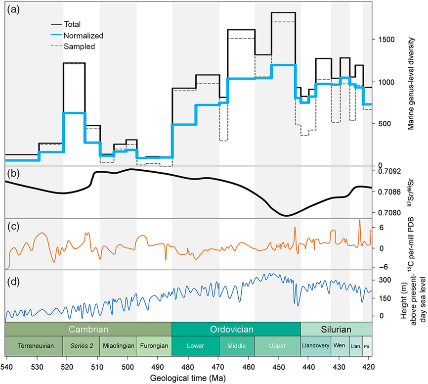
Strontium isotopes have also been analysed in order to understand biodiversification trends at a global level. The very strong shift of ⁸⁷Sr/⁸⁶Sr during Middle–Upper Ordovician time (Fig. 6) appears just before the highest diversities recorded during early Palaeozoic time, and also coincides with the establishment of reef systems in low latitudes during this time interval. Another important ⁸⁷Sr/⁸⁶Sr shift was recorded at the end of Cambrian Stage 2. How can these important shifts, most probably reflecting changes in continental weathering (and therefore plate tectonic events), be related to marine biodiversifications? There is no generally accepted interpretation so far.

Have there been major tectonic, magmatic or volcanic events that interacted with the biodiversification at a global scale? Barnes (Reference Barnes, Webby, Paris, Droser and Percival2004) discussed the possible presence of a mantle superplume during Ordovician time, but evidence for such a plume does not exist, even if modelling studies indicate that such a mantle plume, and its related Large Igneous Province (LIP), could have first resulted in a global warming during Late Ordovician time (the ‘Boda Event’ of Fortey & Cocks, Reference Fortey and Cocks2005) and subsequently the Late Ordovician mass extinction (Lefebvre et al. Reference Lefebvre, Servais, François and Averbuch2010). Similarly, the early Cambrian Kalkarindji continental flood basalt province in northern Australia may have had a severe effect on the earliest Cambrian biota (e.g. Evins et al. Reference Evins, Jourdan and Phillips2009). These LIPs, if they existed, most probably had a similar impact on the biodiversity levels, probably leading to extinctions, as for later mass extinction events (see discussion in Lefebvre et al. Reference Lefebvre, Servais, François and Averbuch2010).

Among all the many possible triggers that have been related to the global increase in marine diversity, the obvious candidate of sea-level change stands out. There is general agreement that global sea levels rose steadily between the late Precambrian Eon and the Late Ordovician Period. Moreover, this long-term sea-level change appears to clearly track increasing marine biodiversity (e.g. Rasmussen et al. Reference Rasmussen, Kröger, Nielsen and Colmenar2019, fig. 3). Figure 6 indicates that, according to the most recent models on sea-level change, the sea level rose continuously until the early Katian Age, matching the increase in marine biodiversity. Both the drop in sea level after that interval and some of the Late Ordovician extinctions appear to start earlier than the Hirnantian Age. Highest sea levels seem to correlate with highest diversities (in the lower and middle parts of the Upper Ordovician strata). This observation also confirms the observation of Smith (Reference Smith2001) who noted that diversity throughout the entire Phanerozoic can be related to sea level, with lower diversities indicating regressions and radiations taking place during transgressions.

This continuous, long-term sea-level rise between the early Cambrian and the Late Ordovician periods may also be related to the palaeogeographical position of the major continents, and in particular those sited at low latitudes. The fragmentation of the Precambrian supercontinent Rodinia continued during the Cambrian–Ordovician interval, giving rise to a greater number of continents; these included several microcontinents located at low to middle latitudes where speciation is usually high, even in modern oceans. This continental fragmentation spawning numerous microcontinents and large epicontinental seas at low latitudes, together with the high sea levels, generated an increase of tropical shelf areas to a maximum at 450 Ma, that is, during the Katian Age (Late Ordovician), before an amalgamation of some microcontinents and continents during latest Ordovician time (Rasmussen & Harper, Reference Rasmussen and Harper2011) and a decline of these epicontinental seas until the end of Silurian time (Walker et al. Reference Walker, Wilkinson and Ivany2002). It is generally assumed that speciation is particularly high in the areas of tropical shelves (such as present-day Indonesia); the increasing size of such areas probably led to the highest diversities and also the construction of reef-building ecosystems during Ordovician time, culminating during the early Late Ordovician Period. These factors are indicative of the long-term, but continuous, evolution of the geosphere, reflected most probably in the long-term radiation of marine organisms. The major pulse of diversifications was also conditioned by the position of the palaeocontinents. The GOBE started in South China during Early Ordovician time (Rong et al. Reference Rong, Fan, Miller and Li2007), while the major pulse on Baltica only took place during Middle Ordovician time when the continent had moved into low latitudes. Additional radiations took place on the Laurentian continent even later, such as during the Richmondian invasion (Stigall, Reference Stigall2010) that involved the coordinated invasion of some 60 genera and, after a speciation gap, intensive niche differentiation and speciation (Stigall, Reference Stigall2019). Numerical analyses of the distribution of the GOBE in time–space has suggested that the early diversifications were an aggregation of local and regional events, whereas those during the Darriwilian Age and later were more global (Franeck & Liow, Reference Franeck and Liow2019). The latter data are mainly based on biota from Baltica and Laurentia and, hypothetically, when other areas are captured in sufficient detail, the scenario of diachronism across groups and regions may have continued into the Silurian Period.

It therefore appears that the major driver of the long-term radiation that can be observed between the late Precambrian Eon and the Early Devonian Period is the palaeogeographical configuration, with continental fragmentation, and the presence of large epicontinental seas near the equator. The palaeogeographical scenario was also most probably related to the general climate conditions, leading to a long-term cooling event during the Ordovician Period (e.g. Nardin et al. Reference Nardin, Goddéris, Donnadieu, Le Hir, Blakey, Puceat and Aretz2011; Pohl et al. Reference Pohl, Donnadieu, Le Hir, Buoncristiani and Vennin2014). The palaeogeographical configuration was also responsible for the global oceanic circulation pattern, including the generation of upwelling zones (Servais et al. Reference Servais, Danelian, Harper and Munnecke2014; Pohl et al. Reference Pohl, Nardin, Vandenbroucke and Donnadieu2016).