


1. Introduction
The evolution of the density of firn with depth is usually related to mean annual air temperature, accumulation rate and surface density (Herron and Langway, Reference Herron and Langway1980; Maeno and Ebinuma, Reference Maeno and Ebinuma1983; Martinerie and others, Reference Martinerie, Raynaud, Etheridge, Barnola and Mazaudier1992), overburden pressure (Kameda and Naruse, Reference Kameda and Naruse1994) or surface winds (Craven and Allison, Reference Craven and Allison1998). Our comprehension of firn densification is related to our understanding of the mechanical properties of snow and ice (e.g. Bartelt and von Moos, Reference Bartelt and von Moos2000; Schneebeli and Sokratov, Reference Schneebeli and Sokratov2004; Faria, Reference Faria2018), the mechanisms of snowpack metamorphism (Bartelt and Lehning, Reference Bartelt and Lehning2002; Schleef and Loewe, Reference Schleef and Loewe2013; Schleef and others, Reference Schleef, Lowe and Schneebeli2014), the dynamics of pore close-off (Raynaud and others, Reference Raynaud2007) and the dynamic process of atmosphere chemistry (Grannas and others, Reference Grannas2007; Hutterli and others, Reference Hutterli, Schneebeli, Freitag, Kipfstuhl and Rothlisberger2009; Faria and others, Reference Faria, Freitag and Kipfstuhl2010).
Since the 1950s, there have been many studies devoted to understanding the flow of ice (e.g. Steinemann, Reference Steinemann1954; Glen, Reference Glen1955; Duval and others, Reference Duval, Ashby and Anderman1983; Jacka, Reference Jacka1984; Budd and Jacka, Reference Budd and Jacka1989; Azuma and Goto-Azuma, Reference Azuma and Goto-Azuma1996; Li and others, Reference Li, Jacka and Budd1996; Petrenko and Whitworth, Reference Petrenko and Whitworth1999; Jacka and Li, Reference Jacka and Li2000; Durham and others, Reference Durham and Stern2001; Goldsby and Kohlstedt, Reference Goldsby and Kohlstedt2001; Hooke, Reference Hooke2005, Song and others, Reference Song, Cole and Baker2006a, Reference Song, Cole and Baker2006b, Reference Song, Baker and Cole2008; Treverrow and others, Reference Treverrow, Budd, Jacka and Warner2012; Hammonds and Baker, Reference Hammonds and Baker2016, Reference Hammonds and Baker2018). There have also been many studies on the deformation of snow and firn (Landauer, 1958; Mellor, Reference Mellor1975; Salm, Reference Salm1982; Maeno and Ebinuma, Reference Maeno and Ebinuma1983; Ambach and Eisner, 1985; Ebinuma and Maeno, Reference Ebinuma and Maeno1985; Meussen and others, Reference Meussen, Mahrenholtz and Oerter1999; Bartelt and von Moos, Reference Bartelt and von Moos2000; Theile and others, Reference Theile, Lowe, Theile and Schneebeli2011).
The work noted above on snow/firn/ice mechanics paved a road to studies relating the deformation of natural snow/firn to high-resolution microstructural observations. While earlier work used optical microscopy to characterize firn (Gow, Reference Gow1969; Alley, Reference Alley1980; Duval and Lorius, Reference Duval and Lorius1980; Thorsteinsson and others, Reference Thorsteinsson, Kipfstuhl, Eicken, Johnsen and Fuhrer1995; Alley and Woods, Reference Alley and Woods1996; Gay and Weiss, Reference Gay and Weiss1999), since Lundy and Adams (Reference Lundy and Adams1998) first examined the microstructure of snow using X-ray microcomputed tomography (micro-CT), there have been several efforts to characterize the microstructure of snow and firn using a micro-CT (Coleou and others, Reference Coleou, Lesaffre, Brzoska, Ludwig and Boller2001; Flin and others, Reference Flin2005; Kaempfer and others, Reference Kaempfer, Schneebeli and Sokratov2005; Kaempfer and Schneebeli, Reference Kaempfer and Schneebeli2007; Flin and Brzoska, Reference Flin and Brzoska2008; Freitag and others, Reference Freitag, Kipfstuhl and Faria2008; Kerbrat and others, Reference Kerbrat2008; Chen and Baker, Reference Chen and Baker2009; Lomonaco and others, Reference Lomonaco, Albert and Baker2011; Lomonaco and Baker, Reference Lomonaco and Baker2013; Wang and Baker, Reference Wang and Baker2013, Reference Wang and Baker2014; Wiese and Schneebeli, Reference Wiese and Schneebeli2017; Burr and others, Reference Burr2018). Wang and Baker (Reference Wang and Baker2013) used both continuous and interrupted compression tests in situ in a micro-CT on snow densities ranging from 100 to 350 kg m−3 at −6°C. They found that the deformation of this low-density snow was a combination of fracturing and sintering but with the sintering predominating. Schleef and Loewe (Reference Schleef and Loewe2013), using in situ micro-CT observations, demonstrated an increase in densification with higher applied stresses and lower initial densities at −20°C, and found that the decrease of the specific surface area with time was independent of the density. Wang and Baker (Reference Wang and Baker2014) investigated the structural evolution of low-density snow under high-temperature gradients (100–500°C m−1) using a micro-CT. They found that the specific surface area was controlled by grain growth and the formation of complex surfaces dominating the specific surface area evolution. Gregory and others (Reference Gregory, Albert and Baker2014) examined the nature of pore closure in firn cores from both the West Antarctic Ice Sheet Divide and Megadunes in East Antarctica using a micro-CT. They found that the open pore structure played a more important role than the density in predicting gas transport properties. Wiese and Schneebeli (Reference Wiese and Schneebeli2017) showed that the settlement of snow under isothermal conditions and a constant temperature gradient of 43°C m−1 was faster than that for other temperature gradients using a micro-CT. Burr and others (Reference Burr, Lhuissier, Martin and Philip2019) using a micro-CT found an abnormal decrease of connectivity with increasing density in Antarctic firn samples at −10°C. They supposed that densification of firn was related to dislocation glide and diffusional processes and not to viscoplastic deformation. Scanning electron microscopy (SEM), which has a higher resolution than using a micro-CT, has also been used to characterize both snow (Iliescu and Baker, Reference Iliescu and Baker2002; Lomonaco and others, Reference Lomonaco, Chen and Baker2009) and firn (Baker and others, Reference Baker, Obbard, Iliescu and Meese2006, Reference Baker, Obbard, Iliescu and Meese2007a, Reference Baker, Sieg, Spaulding and Meese2007b; Lomonaco and others, Reference Lomonaco, Chen and Baker2008; Mayewski and Hamilton, Reference Mayewski and Hamilton2010; Lomonaco and others, Reference Lomonaco, Albert and Baker2011; Spaulding and others, Reference Spaulding, Meese and Baker2011). However, because the SEM is destructive (unlike micro-CT examination), the same sample cannot be examined before and after mechanical testing and in situ deformation experiments would be very challenging. SEM observations also are only from a surface.
At the apex of a polar dome, firn undergoes mainly vertical compression. Below a few meters the load is supplied by the overburden of snow layers. Macroscopically, the stress occurring in ice-sheet flow is typically <0.1 MPa (e.g. Weikusat and others, Reference Weikusat, Kuiper, Pennock, Kipfstuhl and Drury2017), while that in firn is much less than that, since load increases with overburden pressure. However, microscopically, localized stress concentrations at the grain–grain contact areas can be quite high, as noted by Kipfstuhl and others (Reference Kipfstuhl2009) and Faria and others (Reference Faria, Weikusat and Azuma2014). To understand the flow law of a large icy body, such as ice cap or ice sheet, it is insufficient to study a single or discrete sample. Thus, we have performed a systematic observation of creep along a whole firn core.
The firn densification process is usually divided into three stages based on two critical densities, which are 550 and 820–840 kg m−3 (Alley, Reference Alley1987; Ebinuma and Maeno, Reference Ebinuma and Maeno1987; Freitag and others, Reference Freitag, Wilhelms and Kipfstuhl2004). In this work, only the second stage was examined, that is, plastic deformation-induced (creep) compaction. Such creep is typically accommodated by either the motion of crystal lattice defects (dislocations) or diffusive mass transfer (Frost and Ashby, Reference Frost and Ashby1982). We performed constant-load compressive creep tests on firn samples with different densities at different stress levels at −10°C. We characterized the firn microstructures before and after creep testing using both X-ray microcomputed tomography (micro-CT) and thin sections viewed between crossed polarizers.
2. Samples and instruments
2.1 Samples
An ~80 mm diameter, 80 m long firn core, was drilled at Summit, Greenland (72°35′N, 38°25′W), in June 2017, and transported to the US Army Corps of Engineers Cold Region Research Engineering Laboratory, Hanover, NH, where it is stored at −30°C. Immediately prior to testing, samples were completely enveloped with food wrap to reduce sublimation and stored in the Ice Research Laboratory at Dartmouth College at a temperature of −10°C for 2 d to achieve thermal equilibrium. Firn samples were taken every 10 m along the core. Four cylindrical specimens with a 22 ± 0.5 mm diameter and 50 ± 0.5 mm high for creep tests were produced at each depth using a band saw and a hole saw, and polished using increasingly finer sand papers.
2.2 Creep jigs
Four home-built creep jigs were placed in individual Styrofoam boxes in a cold room maintained at −10 ± 0.5°C. Each uniaxial creep testing system consists of an aluminum base plate and three polished aluminum-guide rails passing through linear bearings that hold the upper aluminum loading plate (Fig. 1). Note that the friction force between the linear bearings and guide rods is negligible due to the point contact between them. To measure the displacement during a test, a linear voltage differential transducer (LVDT-Omega LD-320: resolution of 0.025%; linearity error of ±0.15% of full-scale output), parallel to the three aluminum-guide rails, was located adjacent to the center of the upper plate, and fixed tightly using a screw through the plate (Fig. 1). The displacement was logged every 5 s using a Grant SQ2010 datalogger (accuracy of 0.1%). A k-type thermocouple (Omega RDXL4SD thermistor: resolution of 0.1°C) was mounted inside each box. Temperatures were logged at 300 s time intervals over the entire test period.
2-D schematic (a) and photograph (b) of home-built compressive creep jigs. See text for details.
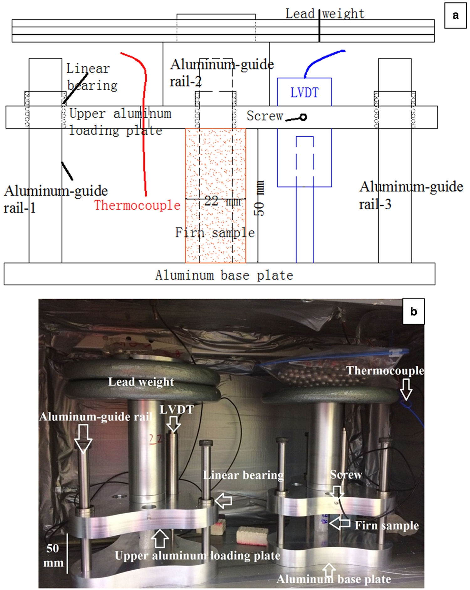
Each creep specimen was placed in the center of the lower aluminum-plate of a creep jig (Fig. 1). During tests, the sample was surrounded by food wrap to reduce sublimation. A constant load was applied to each specimen using weights on the upper plate of the creep jig. Applied stresses from 0.05 to 0.43 MPa were used. Four specimens were tested simultaneously at each depth at four different stresses, i.e. 0.05, 0.11, 0.16 and 0.21 MPa for 10, 20 and 30 m depths; 0.05, 0.16, 0.32 and 0.43 MPa for 40 and 50 m depths; and 0.05, 0.21, 0.32 and 0.43 MPa for 60, 70 and 80 m depths. All tests were run for 500 h except for the 10 m specimen with a stress of 0.21 MPa, which was stopped after 80 h when the displacement exceeded the range of the LVDT. In addition, three tests were performed at stresses of 0.55, 0.65 and 0.75 MPa for 80 m depth for 333 h.
2.3 X-ray microcomputed tomography
Samples before and after creep testing were scanned using a Skyscan 1172 micro-CT, which was housed in a freezer room at −18°C. This cold room temperature enabled a temperature of −10°C to be maintained inside the chamber of the micro-CT, which heats up during scanning due to the heat produced from the X-ray generator. An accelerating voltage of 40 kV was used at a current of 250 μA to provide good contrast for imaging the firn. The image pixel size was set at 17 μm. Scans were performed every 0.7° up to 180° rotation. Each micro-CT scan lasted ~30 min. Each reconstruction consists of 257 projection images. Because the ice phase and the air phase of the firn structure have such different attenuation coefficients, a constant threshold separating the ice phase from the air phase was used throughout. NRecon software was used to transfer a stack of projection images into gray-scale images. After thresholding, binary images were obtained using CTAn software. The cylinder Volume of Interest (VOI, diameter of 12.8 mm; height of 15 mm) was taken from the center of the firn specimen to reduce the cut effect and edge effect. The std dev. of each parameter calculated from the images was from three VOIs, that is the height of VOI was expanded and contracted symmetrically along the specimen by ~0.5 mm.
The microstructural features of interest obtained from the micro-CT data are the density, the structure thickness (S.Th), the total porosity (TP), the closed porosity (CP), the specific surface area (SSA) and the structure model index (SMI).
The percentage object volume is the ratio of volume occupied by ice (Obj.V) to total volume of firn including voids (TV) (Wang and Baker, Reference Wang and Baker2013) in a VOI analytical element. Thus, the density of the firn is calculated from

where ρ ice is the density of pure ice (918 kg m−3).
The S.Th is the mean structure thickness of the ice matrix (Hildebrand and Rüegsegger, Reference Hildebrand and Rüegsegger1997; Chen and Baker, Reference Chen and Baker2010a, Reference Chen and Baker2010b; Wang and Baker, Reference Wang and Baker2013). It represents the largest diameter sphere that encloses a point in the ice matrix and is completely bounded within a solid surface. It represents the characteristic size of the ice particle in the firn.
The total porosity is the ratio of the pore volume including all open and closed pores to the total VOI-calculated volume element. The open porosity is the ratio of the volume of all open pores, which is defined as any space settled in a solid object or between solid objects that has any connection in 3-D to the space outside the object(s), to the total VOI-calculated volume element. The closed porosity is the ratio of the volume of closed pores to the total volume of solid plus closed pores volume in the VOI.
The SSA is the ratio of the ice surface area to total firn volume including the ice and air in a VOI analytical element, and is calculated using the hexahedral marching cubes (Wang and Baker, Reference Wang and Baker2014). It is a parameter that characterizes the thickness and complexity of the firn microstructure. The change of SSA also denotes the change of free-energy of the ice surfaces. Thus, its decrease implies that sintering metamorphism took place under the compressive stress.
The SMI represents the prevalent ice curvature, and is calculated based on the dilation of a 3-D voxel model. It is expressed as (Hildebrand and Rüegsegger, Reference Hildebrand and Rüegsegger1997)

where S and V are the object surface area and volume, respectively, and S′ is the change in surface area due to dilation. SMI values of 0, 3 and 4 represent a flat surface, a cylinder and a sphere, respectively. Negative values represent a concave surface, such as the hollow air structure confined by an ice matrix. The more negative the SMI value, the more sphere-like the pore is.
2.4 Thin section preparation and imaging
Optical photographs were taken of thin sections before and after creep testing. Thin sections were cut from bulk specimens, one side was firstly smoothed with a microtome, and then placed on a 100 × 60 × 2 mm glass plate, and frozen onto it by dropping water along the edge. The thin section was reduced in thickness to ~2 mm with a band saw, and finally thinned further to a uniform thickness of ~0.5 mm using a microtome. The thin section was placed on a light table between a pair of crossed polarizing sheets and digital images were captured using a digital camera.
3. Results and discussions
3.1 Microstructures before creep
Figure 2 shows micro-CT reconstructions of the creep specimens before creep testing for the highest stress specimen at each depth above 70 m and for the 0.43 MPa specimen at 80 m. Under natural loading, the void spaces gradually transform from open to closed, and the number of closed pores increases as the depth increases from 10 to 80 m. As is evident on each cross-section, the closed porosity increases with depth, while the total porosity decreases with depth. The images also show clearly that the fraction of the firn that is ice increases with increasing depth, implying the density increases with depth. It is evident that the polar firn densifies with depth mainly by the sintering-pressure mechanism forced by the accumulated snow load.
Micro-CT 2-D reconstructions of the creep specimens before and after creep testing from 10 m (0.21 MPa) (a), 20 m (0.21 MPa) (b), 30 m (0.21 MPa) (c), 40 m (0.43 MPa) (d), 50 m (0.43 MPa) (e), 60 m (0.43 MPa) (f), 70 m (0.43 MPa) (g) and 80 m (0.43 MPa) (h). The diameter of cross-section is equal to 12.8 mm. The pores are shown in black and the ice in white.

The microstructural parameters obtained from the micro-CT are enumerated in Table 1 and plotted on the ordinate on the graphs in Figure 3. Note that the mean values of these parameters were averaged for the four specimens tested at each depth. However, the 30, 40 and 50 m specimens (named s1, s2, s3 and s4 regardless of stress) were taken from volumes adjacent to the test specimens as these previous data have been mislaid. The std dev. for each microstructural parameter is from the four specimens at each depth (Table 1).
Microstructural parameters before and after creep are for 10 m (a), 20 m (b), 30 m (c), 40 m (d), 50 m (e), 60 m (f), 70 m (g) and 80 m (h). The ordinate respectively is the density (kg m−3), SSA (mm−1), S.Th (mm), total porosity (%), closed porosity (%) and SMI, while the abscissa is the strain (%). The differently colored lines represent the different loads as indicated by the legend on each graph. The standard error indicates the variation of each microstructural parameter.

Microstructural parameters measured by micro-CT before creep at each depth

s1, s2, s3 and s4 denote four different samples before the creep at each depth of 30, 40 and 50 m that were taken from adjacent areas to tested samples.
Several features are worth noting regarding the calculated microstructural parameters. First, as might be expected, the density and structure thickness increase with increasing depth. For example, the average density increased from 511 kg m−3 at 10 m to 861 kg m−3 at 80 m, while the average structure thickness increased from 0.35 to 1.2 mm over the same range. Second, as might be expected, the specific surface area and total porosity decrease with increasing depth. For example, the average specific surface area decreased from 4.7 mm−1 at 10 m to 1.3 mm−1 at 80 m, while the average total porosity decreased from 0.443 at 10 m to 0.126 at 70 m, and then halved at 80 m to 0.062. Third, the closed porosity decreased with increasing depth from10 to 40 m from 0.0006 to 0.00025, but then increased with increasing depths until it was 0.0412 at 80 m. Note that at 10 m the closed porosity is a very small fraction of the total porosity (0.001), whereas at 80 m the closed porosity is 0.66 of the total porosity. Fourth, the structure model index values change from being slightly positive at 10 m to becoming increasingly negative with increasing depth, indicating a change from convex structures to concave structures, which is consistent with a change from open structure to closed pores. Finally, there is scatter in each of the above parameters between the four samples measured at each depth that is greater than the error bars for one specimen, indicating the heterogeneity of the microstructure. However, this scatter decreases with depth, see for example the density values.
3.2 Microstructures after creep
Figure 2 also shows micro-CT reconstructions of the specimens after creep testing for selected samples. The increasing consolidation of the ice matrix (increasing size of the ice particles and increased density), and the decreasing connectedness of the pores and decreased total porosity are evident after the creep tests for the shallow specimens because they suffered large strain, but are less evident visually for the deeper samples, which suffered smaller strains.
Figure 4 compares thin sections before and after creep testing for a load of 0.43 MPa on 60 m firn. It is evident that recrystallization occurred during creep testing. There is no doubt that recrystallization occurred in many of the specimens crept, whereas recrystallization did not occur due to the relative low stresses. However, since we could not determine the occurrence of recrystallization using the micro-CT, and thin sections could only be used at the end of a test – even that was difficult for specimens from shallow depths with large strains since they were quite friable – we do not know when recrystallization initiated during each test. Note that as shown in Figure 4 recrystallization with finer grain sizes was observed in specimens when secondary creep occurred compared to coarser grain sizes before creep. Interestingly, the onset of recrystallization is often assumed to coincide with secondary creep in ice (e.g. Wilson and others, Reference Wilson, Peternell, Piazolo and Luzin2014; Chauve and others, Reference Chauve, Montagnat and Vacher2015), whereas recrystallization data collected across ice and other minerals indicate that recrystallization begins even during primary creep, at 40–95% of the strain required for the strain rate minimum (or stress peak) (Cross and Skemer, Reference Cross and Skemer2019). This is a subject worthy of further study.
Optical photographs of thin sections before (a) and after creep (7.6% strain) (b) for 60 m sample at a load of 0.43 MPa.

3.3 Change of microstructural parameters
Figure 3 shows graphs of various microstructural parameters derived from the micro-CT reconstructions after creep tests.
The density had increased and the total porosity had decreased after creep in most cases but at different rates. In ~9% cases (0.05 MPa at 20 m, and 0.21 and 0.32 MPa at 70 m), there was little change in density or the total porosity, and in ~19% cases (all loads at 50 m, and 0.05 and 0.21 MPa at 80 m), the density decreased and the total porosity increased.
The specific surface area had decreased and the structure thickness had increased after creep in most cases. For ~6% cases (0.11 and 0.16 MPa at 10 m), little change occurred in the specific surface area, and in ~9% cases (0.11 and 0.16 MPa at 10 m, and 0.43 MPa at 50 m), little change occurred in the structure thickness, while for ~9% cases (0.32 MPa at 70 m, and 0.05 and 0.21 MPa at 80 m), the specific surface area increased and the structure thickness decreased.
There was no clear trend in the closed porosity after the creep tests compared to before the tests. In half the tests it increased while in others it decreased. Its decrease might be related to (1) the rupture of closed pores, and (2) the small specimen size and the problem of detection limit of the micro-CT (Burr and others, Reference Burr, Lhuissier, Martin and Philip2019).
The structure model index decreased after creep in more than half the cases as might be expected. However, for ~6% cases (0.21 and 0.32 MPa at 70 m), there was little change, while for ~28% cases (0.05 MPa at 20 m, 0.05 MPa at 30 m, all loads at 50 m, 0.05 and 0.21 MPa at 80 m), the structure model index had increased slightly after creep.
Decreases of the specific surface area and the total porosity generally accompanied the increase of density. However, some exceptions occurred, e.g. for all specimens at 50 m and specimens of 0.05 and 0.21 MPa at 80 m where both the specific surface area and the total porosity increased along with the decrease of density. Note the exceptions and small changes in microstructural parameters are probably related to the volume expansion of specimens resulting either from the unconfined compression or from the non-uniform distribution of local stress in firn (Landauer, 1958; Meussen and others, Reference Meussen, Mahrenholtz and Oerter1999).
In summary, the specific surface area, the total porosity and the structure model index decreased, while the structure thickness increased with increasing density in most cases. These microstructural characteristics are consistent with the densification of the firn.
3.4 Effective stress
The porosity decreases with increasing depth and generally becomes lower after compaction compared to before compaction. Thus, one can differentiate between the applied stress and an effective stress that arises due to the porous nature of the firn samples. The applied stress is the applied load divided by the cross-sectional area of a sample. We define the effective stress as the applied load divided by the mean cross-sectional area of the ice matrix. The latter can be simply calculated by reducing the cross-section due to the total porosity (Chen and Chen, Reference Chen and Chen1997; Lade and de Boer, Reference Lade and de Boer1997; Ehlers, Reference Ehlers, Ehlers and Bluhm2002; Khalili and others, Reference Khalili, Geiser and Blight2004; Gray and Schrefler, Reference Gray and Schrefler2007; da Silva and others, Reference da Silva, Schroeder and Verbrugge2008; Nuth and Laloui, Reference Nuth and Laloui2008). Note that the firn was regarded as the dry two-phase porous media comprised of interconnected ice matrix and air. Also, the changes in the firn, including the spatial variation of porosity, the deformation of the ice matrix, the air pressure in pores, compressibility of both the individual ice grain and the ice skeleton, and volume change during testing, were not taken into account on their influences to the effective stress.
Thus, we calculated values of the effective stress of 0.05–0.57 MPa before testing and 0.05–0.53 MPa after testing. The values for each specimen at each depth are listed in Table 2, together with corresponding values of the applied stresses from 0.05 to 0.43 MPa. In addition, the three higher applied stresses used on specimens from a depth of 80 m of 0.55, 0.65 and 0.75 MPa yield effective stresses of 0.59, 0.7 and 0.8 MPa, respectively. The difference between the applied stresses and the effective stresses has little effect on our later discussions. Thus, only applied stresses are discussed.
The applied stresses and the corresponding effective stresses before and after testing at each depth for depths of 10–80 m

3.5 Relationship between strain and time
Figure 5 shows the strain versus time creep curves for specimens taken every 10 m from 10 to 80 m. As noted in the experimental section, four specimens with different applied initial stresses were tested at each depth (except for 80 m, where seven samples with different loads were tested): the applied stresses generally increased with increasing depth. Each creep curve has an initial elastic deformation region: the elastic strain is larger as the applied stress is increased for the samples at each depth, but is only a small part of the overall strain (Ashby and Duval, Reference Ashby and Duval1985).
Graphs of strain versus time for 10 m (a), 20 m (b), 30 m (c), 40 m (d), 50 m (e), 60 m (f), 70 m (g) and 80 m (h-1, h-2) firn samples at the applied stresses indicated. The dashed lines are curves fitted using Eqn (1) for the primary creep regime.

In general, creep curves for firn can be divided into three types based on the change of rate of strain increase with time, see labels in Figure 5. Type I creep curves show non-steady, decelerating creep (primary or transient creep) initially, followed by quasi-viscous steady-state creep stage (Glen, Reference Glen1955). Type II behavior shows a continuous decelerating creep trend, i.e. transient creep, while Type III shows discernible primary and obvious steady-state creep followed by accelerating (tertiary) creep stage. In the present work, 62.9% curves were Type I (unlabeled on Fig. 5 to keep the graph concise), with 17.1% curves showing Type II behavior, i.e. for 0.11, 0.16 and 0.21 MPa at 10 m, for 0.21 MPa at 20 and 30 m, and for 0.43 MPa at 40 m, while 20% curves showed Type III behavior, i.e. for the specimens which had applied stresses ⩾0.43 MPa at 80 m, and 0.43 MPa from 50 to 70 m. That implies that different creep mechanisms, e.g. grain boundary sliding (Alley, Reference Alley1987), may dominate in the shallow firn above 10 m when the firn density is <550 kg m−3. It also implies that the grain boundary sliding may occur for firn densities >550 kg m−3 (Goldsby and Kohlstedt, Reference Goldsby and Kohlstedt1997), but with a threshold stress value related to a range of density, where the grain boundary sliding is activated if the threshold stress arrives, such as 0.21 MPa at the density of ~570–641 kg m−3 from 20 to 30 m, or 0.43 MPa at the density of ~693 kg m−3 at 40 m, otherwise inactive.
An initial decreasing strain rate can be caused by an increase in the subgrain-boundary density in ice crystals (Hamann and others, Reference Hamann, Weikusat, Azuma and Kipstuhl2007) or by firn densification accompanying the decrease in total porosity. It can also be interpreted by two different hardening processes. One is the kinematic hardening, which is a recoverable elastic back-stress due to non-uniform distribution of long-range internal stresses arising from the different orientations of the grains (Glen, Reference Glen1955; e.g. Fig. 4), as in the early stage of creep, which impacts the basal slip in individual grains. The other mechanism is non-recoverable isotropic hardening which arises from dislocation dipole formation (Taylor hardening) and forest (or Friedel) hardening caused by dislocation tangles or dislocation walls (Duval and others, Reference Duval, Ashby and Anderman1983; Ashby and Duval, Reference Ashby and Duval1985). However, Ashby and Duval (Reference Ashby and Duval1985) thought that forest hardening was unlikely in terms of the geometry of slip in the ice. An accelerating creep rate may be attributed to the softening from recrystallization by relaxing strain heterogeneities along grain boundaries, and by reorienting grains into easy-slip orientations (e.g. Glen, Reference Glen1955; Hobbs, Reference Hobbs1974; Duval, Reference Duval1981; Jacka, Reference Jacka1984).
There are two types of arrangement of creep curves in Figure 5 at each depth. One type is where the curves are arranged in order of the applied stress. This occurred for tests performed for specimens from 10, 30, 40 and 60 m. The other type is where the curves are arranged not based on the applied stress. This leads to a cross-over in some of the creep curves. This occurred for the tests performed on specimens from 20, 50, 70 and 80 m. These cross-overs imply that other factors, such as the microstructural heterogeneity, impact the densification of the firn. However, all cross-overs, except for that of 0.05 and 0.16 MPa at 50 m, occurred in the first 100 h, implying that both the time and the load (e.g. see 80 m specimens in Fig. 5) eliminate these factors in the early stages of the creep.
For many materials including fully-dense, polycrystalline ice (Glen, Reference Glen1955), Andrade's equation is often used to describe primary creep, i.e. the strain, ε, is related to the time, t, by ɛ = βt 1/3, where β is a constant. In the present work, we used a modified Andrade-like equation (Glen, Reference Glen1955; Barnes and others, Reference Barnes, Tabor and Walker1971; Homer and Glen, Reference Homer and Glen1978) for the primary creep regime:

where k is the time exponent and ɛ0 is the instantaneous (elastic) strain. To analyze the data, the primary creep regime was defined to end when the plots of log strain rate versus strain reached a minimum. Apart from the latter tests, all creep curves were solely in the primary creep regime. Except for the specimens with a loading stress of 0.21 MPa at 10 m, 0.05 MPa at 50, 70 and 80 m, the creep curves were well fitted using this equation, see (black dashed lines on the creep curves) Figure 5, where the k values range from 0.17 to 0.76. The commonly observed k = 0.33 for many materials including fully-dense ice was not observed. Instead, 58% of k values were >0.33, while 42% k values were <0.33.
Glen and Jones (Reference Glen and Jones1967) used ɛ ∝ t k to analyze the shear strain versus time data for the creep of ice single crystals at −50°C and obtained a time exponent of 1.5 ± 0.2 for strains of 0.2–2%. They noted that the time exponent increased for higher strains and was independent of temperature. Later, Jones and Glen (Reference Jones and Glen1968) plotted the same relationship for the creep of single crystals of ice at −60°C, and found a continually increasing creep rate with no apparent strain hardening as found at higher temperatures. They obtained a time exponent of 1.4 ± 0.2 for strains between 0.2 and 5%. They supposed that the time exponent must increase with increasing temperature, assuming it varied with temperature regardless of tension, compression or shear, due to a faster strain rate at a higher temperature. Later, Homer and Glen (Reference Homer and Glen1978) obtained a value of k = 1.9 ± 0.5 from the creep of monocrystalline ice under a stress range of 0.1–2 MPa at temperatures from −20 to −4.5°C, and noted that k increased as the strain increased, even sometimes rising to 5. They thought that the change in k was related to changes in the resolved shear stress acting on the basal plane, in which the c-axis of crystalline rotates with respect to the tensile axis. They also found k = 1.3 ± 0.4 for bicrystals for the same ranges of stress and temperature as for the monocrystalline ice.
Landauer (1958) observed that the k values of 0.15–0.57 for snow were dependent on the initial density in the range 369–626 kg m−3 at −10°C, where k = 1 indicated viscous flow and k = 0 occurred for perfectly elastic behavior. Meussen and others (Reference Meussen, Mahrenholtz and Oerter1999) conducted 56 creep tests on snow and firn, and found little difference in k values obtaining a mean value of 0.6 independent of temperature, density or applied load. More recently, Theile and others (Reference Theile, Lowe, Theile and Schneebeli2011) performed six experiments on round-grained snow with densities from 200 to 350 kg m−3 at −11°C, and obtained a k value of 0.4 using an Andrade-like equation. They argued that Andrade creep was a consequence of several microscopic mechanisms, and all mechanisms contribute to the collective mobility in heterogeneous systems as observed in snow.
In summary, k > 1 indicates that the creep of monocrystalline ice is accelerating, while k < 1 occurs when polycrystal is decelerating in primary creep. A reduction in k from monocrystalline, to bicrystals to polycrystalline ice implies that grain boundaries act to slowdown the deformation rate (Homer and Glen, Reference Homer and Glen1978), which leads to the general conclusion that grains in a full-density polycrystalline ice are less free to deform than in a porous polycrystalline firn (and much less free than in a single crystal or bicrystal). Thus, it is expected that the decelerating (primary) creep in firn should be less severe than in a full-density polycrystalline ice, which translates into expecting k would be >1/3 for the firn. In other words, the values of k > 0.33, obtained at higher stresses at each depth, imply that porous polycrystalline firn deforms much more rapidly than full-density polycrystalline ice due to the rearrangement of grains arising from the grain rotation and breaking of bonds between grains. On the other hand, the values of k < 0.33 imply that the deformation of firn slows down primarily due to the lower stresses applied. However, the k value of 0.22 occurs for 0.32 MPa at 70 m, implying that other factors may also be responsible for the firn deformation, e.g. the effects of impurities (Freitag and others, Reference Freitag, Dobrindt and Kipfstuhl2002). Also, we note that the k value overall increases with increasing stress for the specimens at each depth. However, the k value varies irregularly at different depths/densities. Therefore, we expect that the time dependence of creep depends on the applied stress, or other factors, e.g. the effect of impurities (Freitag and others, Reference Freitag, Dobrindt and Kipfstuhl2002), but not on the density of the firn, where the different k values characterize the different competition between strain hardening and strain softening.
3.6 Relationship of strain rate to strain
Figure 6 shows the log strain rate versus strain plots for the specimens in Figure 5. Note that the blue lines in Figure 6 were composed of discrete values of strain rates that were calculated from the strain difference in unit time (1 h), where the strain data were read every 5 s. Next, the moving averages (orange lines in Fig. 6) were used due to the noise from the discrete values, especially from the 0.05 MPa tests. Also, note that the noise generally decreases with increasing stress for the specimens at each depth. Type II creep curves (17.1%) include only transient creep for 0.11, 0.16 and 0.21 MPa at 10 m, for 0.21 MPa at 20, 30 and for 0.43 MPa at 40 m. In particular, the steep decrease of strain rate with increasing strain for the specimens at 10 m implies that the dominant creep mechanism is different from that for the specimens crept at other depths. Type III creep curves (20%) include transient, secondary and tertiary creep for 0.43 MPa at 50, 60 and 70 m, and for the 80 m specimens which had applied stresses ⩾0.43 MPa. Other tests are type I creep curves (62.9%) which include only transient and secondary creep. However, an exception that secondary creep did not occur for 0.05 MPa at 50 m is possibly attributed to the following reasons. The strain rate generally increases with increasing applied stress for a given strain at each depth beyond the cross-over regions noted above. As noted in Section 3.4, the strain rate for 0.05 MPa was always higher than that for 0.16 MPa at 50 m before the appearance of their cross-over. The unusual creep behavior under both loads above may be related to the changes in the firn structure before testing, where the pre-deformed and partially annealed firn more likely occurred because the stress distribution and temperature in drilling, extracting, transporting or storing the firn core changed.
Graphs of log strain rate versus strain for 10 m (a), 20 m (b), 30 m (c), 40 m (d), 50 m (e), 60 m (f), 70 m (g) and 80 m (h) firn samples, where the sub-graphs for the different applied stresses indicated at the same depth are labeled sequentially as 1, 2, 3, etc. The blue lines represent the discrete strain rates, which are calculated by extracting the strain data hourly, while the orange lines represent the moving average by 15 moving windows with respect to the strain.

Note that the strain rate minimum was reached at a strain of 2.6 ± 0.28% regardless of the applied stress for the three samples with the highest stresses (0.55–0.75 MPa) at 80 m. In other words, earlier onset of tertiary creep occurs at higher applied stresses for the same depth. These latter specimens had a density of ~861 kg m−3 and a total porosity of 0.062, compared to a density of 918 kg m−3 for fully-dense ice where a strain rate minimum is usually observed at ~0.5–3% strain (Duval, Reference Duval1981; Mellor and Cole, Reference Mellor and Cole1983; Jacka, Reference Jacka1984; Li and others, Reference Li, Jacka and Budd1996; Jacka and Li, Reference Jacka and Li2000; Song and others, Reference Song, Baker and Cole2005, Reference Song, Baker and Cole2008; Cuffey and Paterson, Reference Cuffey and Paterson2010). Most of the strain rate minima occur in the strain range of ~0.5–3%, while the strain rate minimum occurs at a strain of 11.3% for 0.32 MPa at 40 m, 3.8% for 0.32 MPa at 50 m, 7.1% for 0.43 MPa at 50 m and 4.7% for 0.43 MPa at 60 m. Interestingly, tertiary creep occurs almost immediately after the onset of secondary creep at a strain of 2.6 ± 0.28% for specimens with applied stresses of 0.55–0.75 MPa at 80 m. In contrast, tertiary creep either was not observed until a long period of secondary creep or did not occur at all for specimens with applied stresses of <0.43 MPa (Fig. 6). Thus, a threshold stress occurs ~0.43–055 MPa that divides secondary creep behavior into two categories: (1) for stresses of ⩾0.55 MPa, which was used only in the 80 m core, the secondary creep occurs at a fixed strain (2.6 ± 0.28%); and (2) for stresses ⩽0.43 MPa, the secondary creep occurred over a wide range of strains and was sometimes not observed at all.
Except for the 80 m samples at applied stresses of 0.55–0.75 MPa, the strain at which the strain rate minimum occurs increases with increasing stress. This explains the Type II creep curves, i.e. why secondary creep did not occur for the samples from 0.21 MPa at 20 and 30 m, and for 0.43 MPa at 40 m. These indicate that the deformation mechanisms are different to those in solid ice. For firn, deformation presumably occurs not only in the ice particles themselves, but also by rearrangement of the ice particles, sintering and the collapse of pores.
At 0.43 MPa, the strain rate minimum was reached at lower strains at increasing depth, i.e. at ~7.1% at 50 m, ~4.7% at 60 m, ~2.0% at 70 m and ~0.7% at 80 m (Table 3). Table 3 and Figure 7 show both the minimum strain rate ($\dot{\varepsilon }_{{\rm min}}$ ) and the onset strain at the strain rate minimum ($\varepsilon _{{\dot{\varepsilon }}_{{\rm min}}}$
 ) as a function of density from 50 to 80 m for the applied stress of 0.43 MPa, respectively. A numerical relation was separately fitted to $\dot{\varepsilon }_{{\rm min}}$
 and $\varepsilon _{{\dot{\varepsilon }}_{{\rm min}}}$
 for the specimen mean density (ρ; R 2 = 0.95; R 2 = 0.99; Fig. 7) and the following results were obtained:


Both the minimum strain rate and the onset strain at the strain rate minimum versus the mean density of specimens for 50–80 m depths. The line was fitted to the measured data.

The minimum strain rate, the mean density of the firn and the strain at which the minimum strain rate occurred at a stress of 0.43 MPa at depths of 50–80 m

Figure 7, Eqns (4) and (5) show that the minimum strain rate decreases exponentially with increasing density under the same stress, indicating that the strain at which steady flow commences also decreases exponentially with increasing density. This is because the compressibility decreases with increasing density. An approximate linear relationship between the minimum strain rate ($\dot{\varepsilon }_{{\rm min}}$ ) and the onset strain for the strain rate minimum ($\varepsilon _{{\dot{\varepsilon }}_{{\rm min}}}$
 ) is obtained by dividing Eqn (4) by Eqn (5). Furthermore, using Eqn (5) we estimated the onset strain at the strain rate minimum ($\varepsilon _{{\dot{\varepsilon }}_{{\rm min}}}$
 ) to be 27 ± 2.6% for a stress of 0.43 MPa at a depth of 40 m. However, no strain rate minimum was observed experimentally (Fig. 6), possibly because severe deformation of the specimen, which was up to a strain of ~30%, significantly influences the creep mechanism. Interestingly, the abrupt drop of the strain rate at the strain of ~30% may indicate the occurrence of microcrack (Fig. 6).
Oscillations in strain rate took place at strains of ~1.2 and ~12.5% for 0.11 MPa at 10 m, and at a strain of ~1% for 0.43 MPa at 60 m. This phenomenon might be due to the cyclic mechanism of recrystallization and recovery (Duval, Reference Duval1981), the easy sliding layer effect (Jonas and Muller, Reference Jonas and Muller1969; Duval and Montagnat, Reference Duval and Montagnat2002; Alley and others, Reference Alley, Clark, Huybrechts and Joughin2005; Horhold and others, Reference Horhold2012; Fujita and others, Reference Fujita2014; Eichler and others, Reference Eichler2017), an abrupt collapse of pores, a temperature anomaly or a slip at the platen-sample interface.
3.7 Relationship of strain rate to stress
The empirical Glen’ law

where $\dot{\varepsilon }$ is the strain rate, A is the temperature- and density-dependent rate factor, σ is the stress and n is the stress exponent, is normally used in describing the creep process in ice. Figure 8 shows the plots of log $\dot{\varepsilon }_{{\rm min}}$
 versus log σ, in which the slope of the fitted line is n = 4.6 ± 0.16, n = 4.1 ± 0.37, n = 4.3 ± 0.33/0.34 and n = 4.3 ± 0.21 from the samples of 50–80 m, respectively. There is little difference in the stress exponent n whether the applied stress or the effective stress is used. Here, the analysis of n is performed only for the 50–80 m firn specimens due to two considerations. First, the minimum creep rate for the 0.05 MPa stress was excluded at each depth because it causes a significant non-linear relationship of log $\dot{\varepsilon }_{{\rm min}}$
 versus log σ. Second, using only two minimum strain rates at each depth of 20–40 m is far less reliable for estimating n using Eqn (6).
Log strain rate versus both log applied stress and log effective stress for the 50 m (a), 60 m (b), 70 m (c) and 80 m (d) firn core at stresses excluding data from the 0.05 MPa specimens at each depth, where a minimum strain rate is observed. The stress exponents indicated were obtained for both the applied stress (black color) and the effective stress (green color). The broken line denotes a fitted line from measured data.

In laboratory experiments, Glen and Jones (Reference Glen and Jones1967) performed creep tests on monocrystalline ice in uniaxial tension at −60°C, and obtained an n of 4 ± 1 within strains of 5%. They believed that <11$\bar{2}$ 0> was the glide direction although Kamb (Reference Kamb1961) theoretically argued that the true glide direction, which was related to a-axis, should not be apparent if 3 < n < ~5. Also, they mentioned that the glide direction was associated with the stress and the active slip systems. Goldsby and Kohlstedt (Reference Goldsby and Kohlstedt1997) obtained a stress exponent n = 4 for the creep of fine-grained polycrystalline ice (diameter >40 μm) at −37°C at high stresses. They argued that the multiple slip systems including the hardest one must be activated to satisfy the von Mises criterion. Goldsby and Kohlstedt (Reference Goldsby and Kohlstedt2001) found a creep rate enhancement regime for fine-grained ice at temperatures above −15°C with n = 4.0, where the faster rate of dislocation creep was independent of grain size but caused by premelting at grain boundaries or three- and four-grain junctions at temperatures below the freezing point. Glen (Reference Glen1955) obtained an n = 4.2 from tests on polycrystalline blocks of ice at −0.02°C between 0.15 and 1 MPa, implying that it is more likely to be linked to the melting at the grain boundaries and junctions when tests were performed at very close to melting point temperature.
Based on field observations, Raymond (Reference Raymond1973) found an n ≈ 4 in an analysis based on the spatial variations of deformation for Athabasca Glacier in the Canadian Rockies. Thomas and others (Reference Thomas, MacAyeal, Bentley and Clapp1980) analyzed the flow and morphology of Roosevelt Island, Antarctica, and found n in the range 3–4. Cuffey (Reference Cuffey and Knight2006) obtained n in the range 3–6 when analyzing the surface profiles between the margins and the central divides of polar areas. Bons and others (Reference Bons2018) obtained a stress exponent of 4 by fitting the observed state of the Greenland Ice Sheet. They expected that the ice sheet responded faster in the areas of both the large ice streams and marginal ice than in the interior northern ice sheet currently frozen to bedrock.
Weertman (Reference Weertman1985) explained that for n ⩾ 3, the creep rate was proportional to the product of the dislocation density and the average dislocation velocity, i.e. the former was proportional to the stress squared, and the latter was proportional to the first or higher power of the stress. According to Weertman's hypothesis, the creep rate was possibly enhanced, where both the dislocation density and the average dislocation velocity are both dependent on the stress squared, because the porous firn provides a lesser constraint or higher degrees of freedom for grain deformation (Michel, Reference Michel1978) than in ice.
It is possible that applied stresses on the firn specimen increase the resolved shear stresses on all possible slip planes to enhance the strain rate with n > 4. Alternatively, the fabric and impurities undetermined in the present work may complicate the stress distribution to reduce the viscosity of the firn, and also make n > 4. It is also possible that both the dry friction across the interface of ice particles and internal friction along grain boundaries (Tatibouet and others, Reference Tatibouet, Perez and Vassoille1987; Hatton and others, Reference Hatton, Sammonds and Feltham2009) may also produce heat contributing to the melting of firn to produce an enhanced creep rate.
The values of n deduced in the present work fall into the range of n values observed by others. Dislocation creep dominates the deformation, meaning Glen's law with material parameters similar to those for full-density polycrystalline ice can be applied to describe the creep behavior of high-density firn at relative high stresses (Scapozza and Bartelt, Reference Scapozza and Bartelt2003). Polycrystalline ice deforms by dislocation creep at relative high stresses, but by a transition of significance from dislocation to grain-boundary sliding accompanied with basal glide, Harper-Dorn creep and diffusional creep with decreasing stress. In future work, it will be necessary to advance our experimental understanding of the creep mechanisms at low stress of <0.1 MPa, and low-density firn under constant loads in laboratory experiments.
4. Conclusions
Constant-load creep tests were performed at various stresses at −10°C on specimens taken every 10 m along a firn core extracted at Summit, Greenland in June 2017. The microstructures before and after creep testing were examined using X-ray micro computed tomography and optical images of thin sections. It was found that:
1. The specific surface area, the total porosity and the structure model index (indicating that the curvature of features became more concave) decreased, while the structure thickness (a measure of the ice feature size) increased with increasing density/depth. These changes in microstructures are characteristic of the densification of the firn.
2. An Andrade-like equation, ɛ = βt k + ɛ0 used to describe the primary creep strain yielded k values from 0.17 to 0.76. k values >0.33 (58%) imply that the porous polycrystalline firn deforms much more rapidly than full-density polycrystalline ice due to the rearrangement of grains arising from both grain rotation and the breaking of bonds between grains. k values <0.33 (42%) imply that the deformation of firn slows down primarily due to lower stresses applied.
3. The onset of secondary creep typically occurs in the strain range of ~0.5–3%. The secondary creep behavior can be divided into two categories: (1) for stresses of ⩾0.55 MPa, the secondary creep occurs at a fixed strain (2.6 ± 0.28%); and (2) for stresses ⩽0.43 MPa, the secondary creep occurred over a wide range of strains and was sometimes not observed at all.
4. At a stress of 0.43 MPa from 50 to 80 m, both $\dot{\varepsilon }_{{\rm min}}$
 and the onset strain at which $\dot{\varepsilon }_{{\rm min}}$ occurred decreased exponentially with increasing firn density. There exists an approximately linear relationship between $\dot{\varepsilon }_{{\rm min}}$ and $\varepsilon _{{\dot{\varepsilon }}_{{\rm min}}}$.
5. For the 50–80 m firn, at applied stresses of 0.16–0.75 MPa, the stress exponent, n, in Glen's law $\dot{\varepsilon } = A\sigma ^n$
, was found to be 4.6 ± 0.16, 4.1 ± 0.37, 4.3 ± 0.33/0.34 and 4.3 ± 0.21, respectively. This is similar to the n values previously observed in fully dense ice.6. Micro-CT observations of crept specimens showed that in most cases the specific surface area, the total porosity and the structure model index decreased, while the structure thickness increased with increasing density. These microstructural characteristics are consistent with the densification of the firn.
7. Recrystallization was observed in some specimens that had undergone secondary creep.


In the present work, the microstructures before and after creep testing have been characterized using the non-destructive technique X-ray microtomography. The work contributes to our understanding of how the ice in polar ice sheets is formed from densifying snow/firn and how the air bubbles in ice are formed from the pores in the firn. In future work, it will be necessary to investigate further the quantitative relationship between the creep behavior of polar firn and the microstructural parameters, particularly at different temperatures. Of particular interest is determining why a strain rate minimum does not occur even at strains up to 32% in shallow firn, and at what strains recrystallization is initiated.
Acknowledgements
This work was sponsored by the National Science Foundation Arctic Natural Science grant 1743106. We appreciate the great help to improve this manuscript from Sergio Henrique Faria and another anonymous reviewer. We thank Chris Polashenski, Zoe Courville and Lauren B. Farnsworth at USA-CRREL for their help with the storage of the firn cores. We acknowledge the use of the Ice Research Laboratory (Director – Erland Schulson) at the Dartmouth College.


 Open access