





1. Introduction
Present bias – the desire for immediate gratification – often derails long-term goals such as saving for retirement, starting a diet, or finishing a referee report. Individuals who are present-biased and sophisticated, i.e., aware of their own present bias, can avoid making present-biased decisions by limiting the options they will have in the future (O’Donoghue & Rabin, Reference O’Donoghue and Rabin1999). For example, they might self-impose stringent work deadlines (Ariely & Wertenbroch, Reference Ariely and Wertenbroch2002), invest in illiquid savings products (Ashraf et al., Reference Ashraf, Karlan and Yin2006), sign up for effort-incentivizing contracts (Kaur et al., Reference Kaur, Kremer and Mullainathan2015), or use commitment devices that restrict their future choices (Schilbach, Reference Schilbach2019).Footnote 1 Predicting the dynamic decisions of present-biased individuals, therefore, requires the joint measurement of present bias and sophistication. Yet many empirical studies measure present bias while ignoring sophistication.
The only existing experimental design that directly estimates sophistication, introduced in Augenblick and Rabin (Reference Augenblick and Rabin2019) and extended by Fedyk (Reference Fedyk2024), represents an important contribution. In these designs, participants make real-effort choices at varying wages and predict their future choices; sophistication can be measured by the gap between predictions and actual behaviour.
The identification strategy in these studies, however, relies on the assumption that present bias and sophistication are identical across effort and money domains. This restriction is substantive as prior work documents systematic domain differences. Empirically, present bias has been robustly documented in the effort domain but is often small or statistically insignificant in the money domain (Augenblick et al., Reference Augenblick, Niederle and Sprenger2015; Imai et al., Reference Imai, Rutter and Camerer2021). Conceptually, money is fungible and can be stored or reallocated, whereas effort is non-fungible, immediately experienced, and cannot be deferred or transferred. These differences imply that behaviour associated with exerting effort may be qualitatively distinct from behaviour associated with receiving monetary payments. As we explain in Online Appendix C, imposing a common parameter across domains therefore conflates present bias and sophistication over money and effort, yielding estimates that may fail to capture behaviour in either domain.
Our experiment, conducted online with Prolific participants over 3 days, builds directly on the approach of Augenblick and Rabin (Reference Augenblick and Rabin2019) and Fedyk (Reference Fedyk2024) but introduces a design feature that enables separate identification of present bias and sophistication over money and effort. The key novelty is that all payments are made on Day 3 and this timing is made fully salient to participants. This creates two independent sources of variation. Firstly, we observe choices and predictions when effort costs are immediate (decisions for tasks to be completed on the same day) and when they are delayed (decisions for tasks to be completed on a future day). Comparing choices (and predictions) under immediate versus delayed effort identifies present bias (and sophistication) over effort. Secondly, we observe choices and predictions when monetary benefits are effectively immediate (decisions made on Day 3, paid on Day 3) and when they are delayed (decisions made on Days 1 or 2, paid on Day 3). Comparing choices (and predictions) under immediate versus delayed payment identifies present bias (and sophistication) over money. Thus, our double experimental variation allows us to separately identify present bias and sophistication in the effort and money domains. This contrasts with the designs in Augenblick and Rabin (Reference Augenblick and Rabin2019); Fedyk (Reference Fedyk2024), where all payments are in the future, and hence identifying crucial model parameters requires assuming identical present bias and sophistication across domains.
We begin with a reduced-form analysis, which provides significant evidence for present bias in the effort domain, but little to no evidence for present bias over money. Controlling for the distance between payment and effort dates, participants allocate on average 4.17 (14%) more tasks to future workdays than to the present, but only 0.5 fewer tasks when payment occurs in the future rather than the present – only the former effect is statistically significant. When predicting their own future decisions, participants believe they will allocate 3.09 (rather than 4.17) more tasks to future workdays, providing statistically significant evidence of partial sophistication over effort.
For our structural analysis, we use the quasi-hyperbolic discounting model (Phelps & Pollak, Reference Phelps and Pollak1968; Laibson, Reference Laibson1997) due to its tractability.Footnote 2 We find significant evidence of sophistication over effort ( $\widehat{\beta}_e$): across specifications, the point estimate of $\widehat{\beta}_e$ ranges between 0.80 and 0.88, while the point estimate of present bias over effort ( $\beta_e$) lies between 0.70 and 0.79. Our aggregate estimate of $\beta_m$ ranges between 0.95 and 1.09 and is not statistically different from 1, though substantial individual-level heterogeneity exists, with roughly equal numbers of participants exhibiting present bias and future bias over money. Overall, roughly three quarters of all participants anticipate the direction of their bias in both domains, even if not its full magnitude.
To assess the cost of imposing the common-parameter assumption, we re-estimate our data under Augenblick and Rabin (Reference Augenblick and Rabin2019)’s original restriction. This counterfactual exercise confirms that the assumption biases estimates of key preference parameters: it forces  $\beta$ and $\widehat{\beta}$ mutually closer together than in our preferred specifications, thereby overstating relative sophistication.
Besides serving as a proof of concept for the identification strategy, our 3-day experimental design is more cost-effective, less vulnerable to attrition, and easier to replicate than longer studies. It can moreover be extended to longer horizons or field settings, making it a useful tool for applied researchers who wish to use present bias and sophistication as explanatory variables in domains such as savings behaviour, illiquid investments, gym memberships, and workplace goal-setting.
The remainder of the paper is structured as follows. Section 2 reviews the related literature and situates our contribution within this literature. Section 3 describes the experimental design. Section 4 introduces the model and explains the identification strategy. Section 5 presents our results. Section 6 compares our results with those in closely related previous studies. Section 7 concludes.
2. Literature review
2.1. Measuring sophistication
The literature measuring sophistication about time preferences can be organized into three broad strands. The first strand infers sophistication from individuals’ preferences over commitment devices or restricted choice sets. Ahn et al. (Reference Ahn, Iijima, Le Yaouanq and Sarver2019) provide a behavioural characterization of naïvete based on ex-ante choice over menus and ex-post choice from menus: an individual is sophisticated if she is indifferent ex ante between retaining the option to choose from a menu ex post or committing to her actual distribution of choices from that menu. Other work in this strand treats demand for commitment as a ‘smoking gun’ for sophistication (e.g., Ericson & Laibson, Reference Ericson, Laibson, Bernheim, DellaVigna and Laibson2019; Sadoff & Samek, Reference Sadoff and Samek2019; Sprenger, Reference Sprenger2015). But commitment demand is only an outcome of sophistication, not a direct measure. Moreover, Carrera et al. (Reference Carrera, Royer, Stehr, Sydnor and Taubinsky2022) show that experimentally increasing sophistication can actually reduce demand for commitment, contradicting the assumption that commitment demand cleanly reveals sophistication (see also Westphal, Reference Westphal2024).
The second strand measures sophistication more directly by eliciting beliefs about future behaviour and comparing them to realized behaviour. Augenblick and Rabin (Reference Augenblick and Rabin2019) and Fedyk (Reference Fedyk2024) use incentivized real-effort experiments in which participants decide how much to work at different times under varying wages; sophistication is measured by comparing actual work decisions on future dates with participants’ earlier predictions of those same decisions. Both studies find that participants are naïve about their own present bias: they fail to fully anticipate it, leading them to work less than they had predicted. Fedyk (Reference Fedyk2024) further shows that participants are more sophisticated about others’ present bias than about their own, a phenomenon they call ‘asymmetric naïvete’.
Survey-based approaches also belong to this strand. For example, Cobb-Clark et al. (Reference Cobb-Clark, Dahmann, Kamhöfer and Schildberg-Hörisch2024) classify individuals according to the consistency between their ideal, expected, and actual body weight 1 year later. While intuitive, such proxies can misclassify behaviour. For instance, someone who predicts they will not reach their ideal weight would be labelled sophisticated, even if they are simply unmotivated by the goal. More fundamentally, such survey-based classifications do not yield structural parameters such as  $\beta$ and $\hat{\beta}$. Sial et al. (Reference Sial, Sydnor and Taubinsky2023) link forecast errors to memory biases, finding that individuals who over-report past attendance are less aware of their time inconsistency. The present paper belongs to this second strand, using incentivized measures of precise behaviours and predictions thereof, while extending prior work by allowing present bias and sophistication to differ across effort and money domains.
The third strand relies on proxies or unincentivized measures of sophistication, such as cognitive ability or related psychological traits. For example, Zhang and Greiner (Reference Zhang and Greiner2021) link cognitive ability to awareness of present bias.
2.2. Identification of time preference parameters
A distinct but related body of work addresses identification challenges in estimating time-preference parameters from intertemporal choice data. Strack and Taubinsky (Reference Strack and Taubinsky2026) highlight important challenges in ‘revision design’ experiments, where participants make intertemporal trade-offs between two periods, deciding first in advance and then again when the time comes. They show that with only ordinal choice data, the same observed behaviour can be rationalized by multiple assumptions about how information about future preferences or constraints is revealed to the decision-maker. They note that when trade-offs are measured in cardinal terms, such as monetary amounts, identification becomes possible. Our design exploits this insight by eliciting choices over monetary amounts across time, enabling us to more precisely recover present bias and sophistication by leveraging variation in participants’ willingness to pay.
2.3. Domain-sensitive time preference parameters
Previous literature shows that time preferences are domain-sensitive. People tend to be more present-biased over primary rewards such as food, juice, or work, while present bias often appears weaker – or even absent – for monetary rewards. For example, Cheung et al. (Reference Cheung, Tymula and Wang2022) show that present bias differs across money, healthy foods, and unhealthy foods.
Of particular relevance to our paper, this domain-sensitivity extends to the money-effort distinction, with evidence suggesting that present bias differs systematically between the two. For example, Augenblick et al. (Reference Augenblick, Niederle and Sprenger2015) find no present bias over money but significant present bias over effort. In a meta-analysis about studies using the Convex Time Budget method, Imai et al. (Reference Imai, Rutter and Camerer2021) show that studies using monetary rewards often show statistically insignificant present bias on average, while effort-based studies tend to report a smaller and significant present bias parameter. Identifying sophistication in Augenblick and Rabin (Reference Augenblick and Rabin2019) and Fedyk (Reference Fedyk2024) requires assuming equal present bias and sophistication over money and effort, thereby yielding estimates that may fail to capture behaviour in either domain. This is what distinguishes the current paper: our experimental design identifies sophistication and effort, without assuming equality across money and effort domains.
3. Experimental design
3.1. Sessions
Fig. 1 illustrates the sequence of events across the 3 consecutive days of a session. On Day 1’s consent form, participants were informed that the study involved real-effort tasks over 3 days. Participants then read the instructions and completed a comprehension quiz assessing their understanding of the study’s structure – namely, its 3-day duration, the £5 bonus for completing all days, and the fact that all payments (for tasks and study completion) would be made on Day 3. Before making any decisions, they were required to complete training tasks to familiarize themselves with the task format and its difficulty. The information about study and payment structures was reiterated on Days 2 and 3 as a reminder, then they made all decisions and predictions, and then they completed any effort tasks scheduled for that day.
Session timeline: the timeline of events within each of the 3 days

Fig. 1 Long description
The flowchart outlines a session timeline across three days. Day 1 includes: 1. Consent and instructions, 2. Comprehension quiz, 3. Training tasks, 4. Decisions and predictions, 5. Effort allocation. Day 2 consists of: 1. Consent, 2. Reminder of the timing of tasks and payments, 3. Decisions and predictions, 4. Effort allocation. Day 3 involves: 1. Consent, 2. Reminder of the timing of tasks and payments, 3. Decisions, 4. Effort allocation, 5. All payments. Arrows indicate the progression from Day 1 to Day 2 and from Day 2 to Day 3.
3.2. Decisions and predictions
Participants were asked to choose and predict the number of time-dated real-effort tasks that they wanted to complete for different wages on the current day and on future days.
Over the 3 days, participants saw 9 decision screens similar to the one shown in Fig. 2. On each of the 9 screens, participants saw 5 different wages or piece rates (1 $p$, 3 $p$, 5 $p$, 7 $p$, and 9 $p$) and had to choose the number of time-dated jobs, between 3 and 13, that they wanted to complete at that wage and on that date. Six of the 9 screens were choice screens, on which participants made their own decisions, while the remaining 3 were prediction screens, on which they predicted the number of jobs their future selves would choose to complete. This means that participants made $5\times 9=45$ decisions in total.
Decision screen for choosing jobs  $J \in \{1, 2, \dots, 13\}$ at 5 wages. At each wage $w$, for the selected $J$, the screen dynamically calculated and displayed the number of tasks $J(J+1)/2$ and the total corresponding payment $wJ$. For example, in the figure above, the participant selected $J=3$ at $w=1$, and hence the screen said ‘3 Jobs: 6 tasks for 3 pence total’

Fig. 2 Long description
This is a screenshot of a decision screen where participants choose a pay rate for tasks to be completed the day after tomorrow. The screen displays five selectable options, each with a horizontal slider bar and a circular marker indicating selection. Options are listed as follows: 1 penny per job: 6 Jobs, 21 tasks for 6 pence total. 3 pence per job: 6 Jobs, 21 tasks for 18 pence total. 5 pence per job: 7 Jobs, 28 tasks for 35 pence total. 7 pence per job: 8 Jobs, 36 tasks for 56 pence total. 9 pence per job: 9 Jobs, 45 tasks for 81 pence total. Each option is presented on its own line with a slider bar to adjust the number of jobs and tasks.
Jobs translated into real-effort tasks at a non-linear rate:  $J$ jobs required completing $J(J + 1)/2$ real-effort transcription tasks (just tasks, henceforth). For example, as seen on Fig. 2, $J=3$ jobs required completing $3(3+1)/2=6$ tasks, $J=5$ jobs required completing $5(5+1)/2=15$ tasks, and $J=13$ jobs required completing $13(13+1)/2=91$ tasks.
As illustrated by Fig. 3, a (transcription) task consisted of typing a sequence of characters into an empty box. If the characters were not typed correctly, an error message appeared and the participant had to retype the characters again. Our transcription tasks resemble those used in Augenblick and Rabin (Reference Augenblick and Rabin2019).Footnote 3
Example of a transcription task. Completing  $J$ jobs meant finishing $J(J + 1)/2$ transcription tasks for a total payment of $Jp$
$Jp$

3.2.1. Increasing marginal cost of jobs
Participants were paid the wage or piece rate based on the number of jobs completed. Thus, even though every job offered the same marginal benefit of piece rate  $p$, the $J$-th job required completing $J(J+1)/2-(J-1)J/2=J$ additional real-effort tasks on the margin. This means that participants have to work more and longer to complete each subsequent job.Footnote 4 This design feature helps aligning the job choice with the canonical assumption of the cost being convex and the net utility being concave in jobs.
Theoretically, this feature should also decrease the frequency of corner solutions, i.e., fewer participants should choose either the minimum or the maximum amount of tasks to complete. The reduction of corner choices makes it easier to estimate structural parameters based on the assumption of internal optima.Footnote 5 The mapping from jobs to tasks was explained in advance, as well as transparently presented to the participants on every decision screen (see Fig. 2).
3.2.2. All choices and predictions
Table 1 summarizes all the decisions made by participants by date.  $J_{t\tau}(w)$ denotes the decisions made on day $t$ about the number of jobs to complete on day $\tau$ at the wage $w$. On Day 1, participants decided the number of jobs to complete on Days 1, 2, and 3, denoted by $J_{11}(w)$, $J_{12}(w)$, and $J_{13}(w)$, respectively. On Day 2, they decided the number of jobs to complete on Days 2 and 3, i.e., $J_{22}(w)$ and $J_{23}(w)$, respectively. On Day 3, they decided how many jobs to complete on Day 3, denoted by $J_{33}(w)$.
Decisions and predictions by date

Table 1 Long description
The table maps when job-count decisions are made and when predictions about those decisions appear, organized by decision date (rows) and work date (columns). On decision date 1, there is a decision for work date 1, and for work dates 2 and 3 the cells include both the decision and a prediction made on decision date 2. On decision date 2, there is a decision for work date 2, and for work date 3 the cell includes both the decision and a prediction made on decision date 3. On decision date 3, there is a decision for work date 3 only. Blank cells indicate no entry for that decision date and work date pairing. The structure implies decisions are made no later than the work date, while predictions are added later for future work dates. Values depend on the wage rate category, but the table does not provide the numeric job counts. $J_{t\tau}(w)$ denotes the decision made on date $t$ about the number of jobs to do on date $\tau$. $\widehat{J_{t\tau}}(w)$ denotes the prediction about $J_{t\tau}(w)$. $w\in \{1, 3, 5, 7, 9\}$ denotes the wage rate.
On each day  $\tau$, one decision was randomly chosen from the pool of decisions made for that day, and participants had to complete the corresponding number of jobs for the corresponding wage. As an example, on Day 3, one decision was randomly drawn from a pool of 15 decisions: decisions $J_{13}$, $J_{23}$, and $J_{33}$, each of them made for 5 different wages.
After making their decisions, participants completed the tasks corresponding to the randomly selected decision for that day. Only after completing these tasks did they proceed to the prediction stage. This temporal separation ensures that decisions and predictions are meaningfully separated in time. $J^p_{t\tau}(w)$ denotes the prediction of the decision $J_{t\tau}(w)$. Participants faced 3 prediction screens. On Day 1, they made predictions $J^p_{22}(w)$ and $J^p_{23}(w)$ about $J_{22}(w)$ and $J_{23}(w)$, respectively. On Day 2, they predicted $J_{33}(w)$.
3.3. Payments
All payments were made within the evening of the third day after the survey was over, as promised in the instructions. To make sure that participants understood all the sources of payment, we quizzed them about the experiment’s payment structure, including one question about the timing of the payments.Footnote 6
There were four sources of payment for each participant. Firstly, participants received a participation fee for each day they participated in the study ( $\unicode{x00A3}2$, $\unicode{x00A3}1$, and $\unicode{x00A3}1$, respectively). The participation fee was higher on the first day than on the other 2 days as participants spent more time reading instructions, completing mandatory tasks for training, and making more decisions. Secondly, participants received a bonus of $\unicode{x00A3}5$ if they completed all 3 days of the experiment. This completion fee was relatively high to minimize attrition. Thirdly, on each day, participants completed tasks and were paid according to one randomly chosen decision out of the decisions they made for that day. To calculate this payment, the randomly drawn wage rate was multiplied by the number of jobs chosen and completed for that decision. On each day, the payment could range from 3 $p$ (1 $p$
$p$  $\times$ 3 jobs) to 117 $p$ (9 $p$
$p$  $\times$ 13 jobs). On the 3 survey days, participants earned 35 $p$, 35 $p$, and 32 $p$ on average for completing their chosen number of transcription tasks, respectively.
Finally, participants could receive a fourth payment of 20 $p$ if one of their predictions (randomly chosen from their 15 predictions) differed by no more than 2 jobs from their actual decision. Thus, on average, every accurate prediction task only paid 1.33 $p$. Around 87% of all predictions were accurate within 2 jobs, and hence qualified for the 20 $p$ reward if chosen for payment. Unlike Augenblick and Rabin (Reference Augenblick and Rabin2019), who reminded participants of their prior predictions before final decisions, we follow Fedyk (Reference Fedyk2024) in omitting such reminders to avoid priming participants to behave consistently with earlier responses.
Setting the prediction reward involved a trade-off. Too large an accuracy bonus would allow sufficiently sophisticated participants to use the prediction tasks as a commitment device, since the prospect of matching a previously made prediction could incentivize their future selves to work harder than wage incentives alone would warrant. Too small a bonus, on the other hand, might lead participants to provide careless predictions.Footnote 7 We therefore set a very small accuracy bonus as a compromise between these two concerns.
3.4. Participants and selection
All experimental sessions were run online in November 2021 and May 2022. With the goal of having a sample of around 100 participants post-attrition, we recruited 138 participants through Prolific. A total of 115 participants completed the study, although 7 had some missing data. In November, the median length of the experiment was 30 minutes on the first day, 15 minutes on the second day, and 9 minutes on the third day. In May, the median length was 27, 12, and 12 minutes, respectively. A total of 108 participants completed all 3 days of the experiment. This study was not preregistered, as the data were collected prior to the widespread adoption of preregistration practices in the field.
Out of the 138 participants who completed the first day of the study, 108 responded to all questions during the 3 days. Of these, 7 participants did not show any variation across any of the 9 screens, leaving 101 participants for meaningful regression analyses. To winsorize this sample, we further excluded the participants who ranked in the top 10% of ‘most frequent violators’ in each of the following categories: wage monotonicity, time-monotonicity with respect to effort date, and time-monotonicity with respect to pay date. Our final dataset therefore consists of 80 participants (out of the 101 regression-eligible). For consistency, and if not otherwise stated, all the tables or graphs that follow use this sample of 80 participants.
The three monotonicity conditions used to define the sample restrictions – wage monotonicity, time-monotonicity with respect to effort date, and time-monotonicity with respect to pay date – are discussed in detail, along with the corresponding statistics, in Online Appendix A.
4. Model and identification strategy
To motivate our analysis of the data, we start with a general model of behaviour where participants (implicitly) trade off the benefits of completing jobs (i.e., the money,  $J w$) with the costs (i.e., the effort that must be exerted). We assume that on decision day $t_d$, participants choose their optimal effort $J^*$ for day $t_e \geq t_d$ on the experimental task with piece-rate $w$ based on the following utility optimization exercise:
 \begin{equation}
J^{\ast}= \arg\max_{J} \psi \beta_m^{\mathbb{1} (3 \gt t_d)} \delta^{3-t_d} J w -
\beta_e^{\mathbb{1} (t_e \gt t_d)} \delta^{t_e-t_d} c\left(J(J+1)/2\right)
\end{equation}
\begin{equation}
J^{\ast}= \arg\max_{J} \psi \beta_m^{\mathbb{1} (3 \gt t_d)} \delta^{3-t_d} J w -
\beta_e^{\mathbb{1} (t_e \gt t_d)} \delta^{t_e-t_d} c\left(J(J+1)/2\right)
\end{equation}where  $c(\cdot)$ is the cost from the $J(J + 1)/2$ transcription tasks that need to be completed for $J$ jobs, as previously described in Section 3.2. The indicator ${\mathbb{1} (3 \gt t_d) }$ denotes whether the payment day (Day 3) is later than the decision day $t_d$. Similarly, $\mathbb{1} (t_e \gt t_d) $ indicates whether the decision is being made about working in the future, and $(t_e-t_d)$ measures the distance between the effort date and the decision date. The scale parameter $\psi$ normalizes the benefit of monetary gains and the cost from transcription tasks at the same unit.Footnote 8
When asked to predict the decision  $J^{\ast}$ at some prediction period $t_p \lt t_d$, participants report:
 \begin{equation}
\hat{J}= \arg\max_{J} \psi \widehat{\beta}_m^{\ \mathbb{1} (3 \gt t_d) } \delta^{3-t_d} J w -
\widehat{\beta}_e^{\ \mathbb{1} (t_e \gt t_d) } \delta^{t_e-t_d} c(J(J+1)/2)
\end{equation}
\begin{equation}
\hat{J}= \arg\max_{J} \psi \widehat{\beta}_m^{\ \mathbb{1} (3 \gt t_d) } \delta^{3-t_d} J w -
\widehat{\beta}_e^{\ \mathbb{1} (t_e \gt t_d) } \delta^{t_e-t_d} c(J(J+1)/2)
\end{equation} To get to Equation ((2)) from ((1)), one simply replaces  $\beta_m$ by $\widehat{\beta}_m$ and $\beta_e$ by $\widehat{\beta}_e$. In Equation ((2)), the first term is the perceived discounted benefit of completing more jobs and the second term is its perceived discounted cost.
4.1. Time-consistent vs. sophisticated vs. naïve
Following O’Donoghue and Rabin (Reference O’Donoghue and Rabin1999), we distinguish between three mutually exclusive types of individuals. When  $\beta_m = \beta_e = 1$, the individual has exponential discounting preferences. In this case, her relative valuation of earlier versus later utility remains constant regardless of when she is asked to make that trade-off. Since there is no conflict between her preferences at different points in time, such a person is said to be time-consistent, and her plans/predictions automatically align with her future actions.
When either  $\beta_m \lt 1$ or $\beta_e \lt 1$, the individual exhibits present bias. When considering trade-offs of utility between two moments, present-biased individuals give stronger relative weight to the earlier moment if it is also in the present. This bias creates the possibility of a divergence between plans/predictions and future actions, depending on whether the individual anticipates her present bias.
O’Donoghue and Rabin (Reference O’Donoghue and Rabin1999) classify individuals as sophisticated or naïve only when they are present-biased (i.e.,  $\beta_m \lt 1$ or $\beta_e \lt 1$). If the individual correctly anticipates her present bias, she is sophisticated; otherwise, she is naïve.
More generally, we interpret sophistication as the accuracy of individuals’ beliefs about their own present-bias parameters,  $\widehat{\beta}_e$ and $\widehat{\beta}_m$, which can be defined irrespective of whether $\beta \lt 1$ or $\beta \geq 1$. A fully sophisticated individual satisfies $\widehat{\beta}_e = \beta_e$ in the effort domain (or $\widehat{\beta}_m = \beta_m$ in the money domain), while deviations between $\widehat{\beta}$ and $\beta$ reflect the degree of naïveté. For completeness, our graphs and tables report both present bias ( $\beta$) and perceived present bias ( $\hat{\beta}$) for all participants, including those with $\beta \geq 1$.
4.2. Identification
Overall, as long as  $c(\cdot)$ is convex in $J$, the problem in Equation ((1)) or ((2)) is strictly concave and has a unique solution. In particular, for our parametric estimation exercise, we will assume that $c(x)= \frac{x^{\gamma+1}}{\gamma+1}$ and substitute it in the first-order condition derived from (2):
 \begin{equation}
\left(\psi \frac{\widehat{\beta}_m^{\mathbb{1} (3 \gt t_d) } w \delta^{3 - t_e}}{\widehat{\beta}_e^{\mathbb{1} (t_e \gt t_d) } } \right) - \frac{2\hat J+1}{2} c'\left(\hat{J}(\hat{J}+1)/2 \right) = 0.
\end{equation}
\begin{equation}
\left(\psi \frac{\widehat{\beta}_m^{\mathbb{1} (3 \gt t_d) } w \delta^{3 - t_e}}{\widehat{\beta}_e^{\mathbb{1} (t_e \gt t_d) } } \right) - \frac{2\hat J+1}{2} c'\left(\hat{J}(\hat{J}+1)/2 \right) = 0.
\end{equation} \begin{equation}
\iff \left(\psi \frac{\widehat{\beta}_m^{\mathbb{1} (3 \gt t_d) } w \delta^{3 - t_e}}{\widehat{\beta}_e^{\mathbb{1} (t_e \gt t_d) } } \right) - \left( \frac{\hat J(\hat J+1)}{2} \right)^{\gamma} \left( \frac{2\hat J+1}{2} \right) = 0.
\end{equation}
\begin{equation}
\iff \left(\psi \frac{\widehat{\beta}_m^{\mathbb{1} (3 \gt t_d) } w \delta^{3 - t_e}}{\widehat{\beta}_e^{\mathbb{1} (t_e \gt t_d) } } \right) - \left( \frac{\hat J(\hat J+1)}{2} \right)^{\gamma} \left( \frac{2\hat J+1}{2} \right) = 0.
\end{equation} Thus, the prediction  $\hat{J}$ directly reflects the individual’s beliefs about her own future preferences, as captured by $\widehat{\beta}_m$ and $\widehat{\beta}_e$. This identification strategy relies on other components – such as the marginal cost function $c'(\cdot)$ – being known. This dependency underscores the importance of the training tasks administered before any decisions were made on Day 1 (see Fig. 1), as they were designed to increase participants’ familiarity with both the overall cost and the marginal cost of performing the tasks. As before, one can move between the optimality conditions for $J^\ast$ and $\hat J$ by interchanging $\beta_m$ with $\widehat{\beta}_m$, and $\beta_e$ with $\widehat{\beta}_e$.
4.3. Our approach
To jointly estimate  $\beta$ and $\widehat {\beta}$ parameters separately for effort and money, our experimental design allows us to independently observe:
• Variation 1: Choices and predictions when the effort costs are in the future (tasks to be completed on later days) versus when the effort costs are immediate (tasks to be completed the same day).
• Variation 2: Choices and predictions when the benefits (payments) are in the future (decisions made on Days 1 and 2, paid on Day 3) versus when the benefits are immediate (decisions made on Day 3, paid the same day).
While other studies such as Augenblick and Rabin (Reference Augenblick and Rabin2019) and Fedyk (Reference Fedyk2024) also use Variation 1, they lack Variation 2, as their payment date is always strictly after every effort date. Thus,  $\beta_m$ and $\widehat{\beta}_m$ can never be identified separately from $\beta_e$ and $\widehat{\beta}_e$, respectively.
Equipped with Variations 1 and 2, and assuming i.i.d. normally distributed errors with equal variance across choice and predictions, we estimate the parameter vector of the model, i.e.,  $\theta = (\beta_e, \widehat{\beta}_e, \beta_m, \widehat{\beta}_m, \delta, \psi, \gamma)$, using the maximum likelihood estimator (MLE) over both choice and prediction data. $\widehat{\theta}_{\text{MLE}}$, the maximum likelihood estimate of $\theta$, is defined as
 \begin{align*}
\widehat{\theta}_{\text{MLE}} & = \arg\max_{\theta} \sum_{f=1}^F \ln \mathcal{L}_f (\theta), \quad \text{where} \nonumber \\
\ln \mathcal{L}_f (\theta) & = \begin{cases}
- \ln \sigma - 0.5 \ln 2\pi - 0.5 \left( \frac{J_f^{\ast}(\theta) - J_f}{\sigma} \right)^2 &\text{For choice data}\\
- \ln \sigma - 0.5 \ln 2\pi - 0.5 \left( \frac{\widehat{J_f(\theta)} - J_f}{\sigma} \right)^2 &\text{For prediction data}
\end{cases}
\end{align*}
\begin{align*}
\widehat{\theta}_{\text{MLE}} & = \arg\max_{\theta} \sum_{f=1}^F \ln \mathcal{L}_f (\theta), \quad \text{where} \nonumber \\
\ln \mathcal{L}_f (\theta) & = \begin{cases}
- \ln \sigma - 0.5 \ln 2\pi - 0.5 \left( \frac{J_f^{\ast}(\theta) - J_f}{\sigma} \right)^2 &\text{For choice data}\\
- \ln \sigma - 0.5 \ln 2\pi - 0.5 \left( \frac{\widehat{J_f(\theta)} - J_f}{\sigma} \right)^2 &\text{For prediction data}
\end{cases}
\end{align*}where  $f$ is an index for choice and prediction data points, combined across all individuals and 3 days for aggregate analysis, and fixing an individual over 3 days for individual-level analysis. For any value of $\theta$, $J_f^{\ast}(\theta), \widehat{J_f(\theta)}$ are calculated using Equation (4). MLE finds the set of parameters $\theta$ that maximizes the joint likelihood of observing the complete data.
5. Results
For the data to be consistent with any rational model of choice, the number of jobs chosen (or predicted to be chosen) should weakly increase with the wage, and should also weakly increase when the work is scheduled for a later day. Online Appendix A shows that these monotonicity conditions (Chakraborty et al., Reference Chakraborty, Calford, Fenig and Halevy2017) hold for the vast majority of our data. Moreover, we also discuss the frequency of corner choices in the data.
5.1. Reduced-form analysis
Following Augenblick and Rabin (Reference Augenblick and Rabin2019), we use the following regression specification at both the aggregate level (Section 5.1.1) and the individual level (Section 5.1.2) to find the marginal effect of present bias over money and effort on effort choices, without imposing any parametric assumptions on the felicity function or discounting. Our regression specification is:
 \begin{align}e_{i,j} &= \phi_0 + \phi_{e}^{\text{future}} 1^{\text{future } e}_{i,j} + \phi_{e}^{\text{predict}} 1^{\text{predict } e}_{i,j} + \phi_{m}^{\text{future}} 1^{\text{future } m}_{i,j} + \phi_{m}^{\text{predict}} 1^{\text{predict } m}_{i,j}\cr
&\ \ + \phi_\gamma w_{i,j} + \phi_{\delta} \left( 3 - t_e \right) + \mu_i + \varepsilon_{i,j}.
\end{align}
\begin{align}e_{i,j} &= \phi_0 + \phi_{e}^{\text{future}} 1^{\text{future } e}_{i,j} + \phi_{e}^{\text{predict}} 1^{\text{predict } e}_{i,j} + \phi_{m}^{\text{future}} 1^{\text{future } m}_{i,j} + \phi_{m}^{\text{predict}} 1^{\text{predict } m}_{i,j}\cr
&\ \ + \phi_\gamma w_{i,j} + \phi_{\delta} \left( 3 - t_e \right) + \mu_i + \varepsilon_{i,j}.
\end{align}where  $e_{i,j}$ is the number of jobs (or tasks) chosen by individual $i$ at observation $j$. Observation $j$ can be either an effort decision or an effort prediction. The regression controls for standard impatience or discounting through $(3 - t_e)$, the relative distance between the payment date and the effort date.Footnote 9 To allow for different base levels of efforts chosen by different individuals, we include participant-level fixed effect terms $\mu_i$ as dummy variables. We also control for the wage rate $w_{i,j}$: $\phi_{\gamma} \gt 0$ captures the wage monotonicity. Conditional on observation $j$ being an effort decision,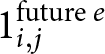 $1_{i,j}^{\text{future } e}$ equals one if $j$ involves future effort, and $1_{i,j}^{\text{future } m}$ equals one if the payment is made in the future. $1_{i,j}^{\text{predict } e}$ and $1_{i,j}^{\text{predict } m}$ are the corresponding indicators when observation $j$ is an effort prediction instead.
For a fixed relative distance  $(3 - t_e)$ between the payment date and the effort date, $\phi^{future}_e$ measures the additional number of jobs that participants choose to complete in the future, relative to the present. A positive value of $\phi^{future}_e$ implies participants choose more effort if it needs to be exerted in the future than if it needs to be exerted immediately, indicating a present bias over effort. The higher is $\phi^{future}_e$, the higher the implied present bias over effort (i.e., the lower is $\beta_e$). Thus, $-\phi^{future}_e$ provides a reduced-form measure that maps to $\beta_e$, with lower values of either corresponding to more present-biased individuals.
Similarly,  $-\phi^{predict}_e$ provides a reduced-form measure of perceived present bias over effort. Sophistication is reflected in how closely perceived present bias aligns with actual present bias.
In the money domain,  $\phi^{future}_m$ measures how effort choices respond to the timing of payments. A negative value of $\phi^{future}_m$ indicates that participants choose fewer jobs when payments are immediate rather than delayed, consistent with present bias over money (i.e., $\beta_m \lt 1$). Thus, $\phi^{future}_m$ provides a reduced-form measure of actual present bias over money, with lower values of either corresponding to more present-biased individuals. Similarly, $\phi^{predict}_m$ captures perceived present bias over money, while the difference between $\phi^{future}_m$ and $\phi^{predict}_m$ reflects the degree of relative sophistication over money ( $\beta^b_m$).
Note that the interpretation of coefficients differs across domains: present bias over effort is reflected in positive values of  $\phi^{future}_e$ and $\phi^{predict}_e$, whereas present bias over money is reflected in negative values of $\phi^{future}_m$ and $\phi^{predict}_m$.
5.1.1. Aggregate analysis
Table 2 shows reduced-form measures of present bias and sophistication over the effort and money domains. As our dependent variable, we use both the number of jobs chosen, which is directly related to the payment (wage) that participants earn, and the number of real-effort tasks.
Reduced-form estimates of present bias and sophistication at the aggregate level

Table 2 Long description
The table reports fixed-effects regression coefficients from aggregate data where the outcome is the number of Jobs or Tasks chosen. In the effort domain, the future-bias coefficient is positive and statistically significant for both outcomes (Jobs 0.52 with standard error 0.13; Tasks 4.17 with standard error 1.11), indicating stronger present bias over effort. The perceived-bias coefficient in the effort domain is also positive and significant but smaller (Jobs 0.33 with standard error 0.15; Tasks 3.09 with standard error 1.32), suggesting people anticipate some bias but less than what is estimated for future choices. In the money domain, both future and perceived coefficients are negative but close to zero and not statistically significant (Jobs about minus 0.05 and minus 0.07; Tasks about minus 0.52 and minus 0.56). Other coefficients show a large, precisely estimated positive effect for both outcomes (Jobs 0.42 with standard error 0.01; Tasks 3.27 with standard error 0.09), while the second is modest and only weakly significant for Tasks (Jobs 0.12 with standard error 0.08; Tasks 1.23 with standard error 0.73). Sample size is 80 units with 3,600 observations for each outcome. Statistical significance is indicated by stars, so non-starred money-domain estimates should be interpreted cautiously as not distinguishable from zero.
Fixed effects regression estimates of Equation ((5)) from aggregate data. The dependent variable is the number of Jobs or Tasks chosen. Present bias over effort is reflected in higher values of  $\phi^{future}_e$, while present bias over money is reflected in lower (more negative) values of $\phi^{future}_m$. The corresponding $\phi^{predict}$ coefficients capture perceived present bias, and the gap between $\phi^{future}$ and $\phi^{predict}$ reflects sophistication.
*** p<0.01; **p<0.05; *p<0.1.
Participants choose  $0.52$ more jobs or $4.17 $ more transcription tasks (which translates to 14% more tasksFootnote 10) to be completed in the future than in the present, but believe that this effect would be smaller ( $0.33$ jobs or $3.09$ tasks), which is evidence of partial sophistication. The difference between $\phi_{e}^{\text{future}}$ and $\phi_{e}^{\text{predict}}$ is not statistically significant. We do not observe a statistically significant degree of present bias in the money domain. Participants choose $0.05$ fewer jobs or $0.52 $ fewer transcription tasks (which translates to 1% fewer tasks) when they are paid on the same day than when they are paid in the future. Neither is significantly different from zero. This result is consistent with findings by Andreoni and Sprenger (Reference Andreoni and Sprenger2012) and Augenblick et al. (Reference Augenblick, Niederle and Sprenger2015), who do not find evidence of present bias over money. While the difference between $\phi_{m}^{\text{future}}$ and $\phi_{m}^{\text{predict}}$ is not statistically significant, we also do not find aggregate evidence for present bias over money in the first place.
5.1.2. Individual analysis
To derive reduced-form measures of present bias and sophistication for each participant, we re-use the regression in Equation ((5)) at the individual level for all 80 participants. Below, we only report the results using the number of jobs, as the results are qualitatively identical if we used the number of tasks instead. This individual analysis is important as average values hide individual differences. As we will see, the data suggest that some individuals are present-biased, others are close to time-consistent, and others again are future-biased. Future studies can use this heterogeneity to predict theoretically related behaviours.
Fig. 4 shows the histogram of reduced-form estimates of actual and perceived present bias in both the effort and the money domains, for all but one participant, who has an outlier estimate of perceived present bias over effort of 12.6. The top-left panel shows the estimates of actual present bias in the effort domain. The  $-\phi_{e}^{\text{future}}$ estimates of around 60% (47 out of 80) participants are below 0, which indicates a modal pattern of present bias over effort. The median is $-0.2$ and the mean is $-0.53$.
The top-right panel shows actual present bias over money. The median and mean of  $\phi^{future}_m$ are roughly zero: $-0.03$ and $-0.06$, respectively. This reflects substantial heterogeneity instead of a modal pattern: 41 and 39 individuals have estimates consistent with present-bias ( $\phi^{future}_m \lt 0$) and future-bias ( $\phi^{future}_m \gt 0$) over money, respectively.
The bottom-left panel shows perceived present bias over effort. The median and mean of  $\phi_{e}^{\text{predict}}$ are $-0.14$ and $-0.17$, respectively. Since these measures are less negative than those of actual present bias, on aggregate, participants are partially sophisticated in our data (also see Fig. 5 for this comparison).
The bottom-right panel shows perceived present bias over money. The median and mean of  $\phi_m^{\text{predict}}$ are $0$ and $0.03$, respectively, suggesting similar heterogeneity to actual present bias over money.
Histograms of reduced-form estimates at the individual level. The panels on the top show estimates of actual present bias, while the panels on the bottom show estimates of perceived present bias based on prediction data. For the effort domain, actual and perceived present bias correspond to  $-\phi^{future}_e$ and $-\phi^{predict}_e$, respectively, so that more negative values indicate stronger present bias. For the money domain, actual and perceived present bias correspond to $\phi^{future}_m$ and $\phi^{predict}_m$, respectively, where more negative values indicate stronger present bias. The median and mean of actual present bias over effort are $-0.2$ and $-0.53$. The median and mean of perceived present bias over effort are $-0.14$ and $-0.17$. The median and mean of actual present bias over money are $-0.03$ and $-0.06$. The median and mean of perceived present bias over money are $0.00$ and $-0.03$. $N=79$ for all figures; one participant with an outlier estimate of $\phi_e^{\text{predict}} \gt 12.6$ is dropped

Fig. 4 Long description
The image A showing a histogram with the horizontal axis label “Actual Present Bias (effort)” and tick labels negative 6, negative 5, negative 4, negative 3, negative 2, negative 1, 0, 1, 2, 3, 4, 5, 6. The vertical axis label is “Density” with tick labels 0, 0.1, 0.2, 0.3, 0.4. Bars are grouped in narrow adjacent intervals across the horizontal axis. The tallest bars are between negative 1 and 0, reaching close to 0.4 density. Many bars appear between about negative 3 and 1, with smaller bars extending to about negative 6 and to about 5. The image B showing a histogram with the horizontal axis label “Actual Present Bias (money)” and tick labels negative 6, negative 5, negative 4, negative 3, negative 2, negative 1, 0, 1, 2, 3, 4, 5, 6. The vertical axis label is “Density” with tick labels 0, 0.1, 0.2, 0.3, 0.4. Bars are grouped in narrow adjacent intervals across the horizontal axis. The tallest bar is around 1, reaching slightly above 0.4 density. Most bars are between about negative 2 and 2, with smaller bars extending to about negative 4 and to about 4. The image C showing a histogram with the horizontal axis label “Perceived Present Bias (effort)” and tick labels negative 6, negative 5, negative 4, negative 3, negative 2, negative 1, 0, 1, 2, 3, 4, 5, 6. The vertical axis label is “Density” with tick labels 0, 0.1, 0.2, 0.3, 0.4. Bars are grouped in narrow adjacent intervals across the horizontal axis. The tallest bars are between negative 1 and 1, reaching close to 0.4 density. Many bars appear between about negative 3 and 2, with smaller bars extending to about negative 6 and to about 5. The image D showing a histogram with the horizontal axis label “Perceived Present Bias (money)” and tick labels negative 6, negative 5, negative 4, negative 3, negative 2, negative 1, 0, 1, 2, 3, 4, 5, 6. The vertical axis label is “Density” with tick labels 0, 0.2, 0.4, 0.6. Bars are grouped in narrow adjacent intervals across the horizontal axis. The tallest bar is around 0, reaching slightly above 0.6 density. Most bars are between about negative 2 and 2, with smaller bars extending to about negative 3 and to about 4.
CDFs of individual-level reduced-form estimates of actual present bias ( $-\phi_{e}^{\text{future}}$ and $\phi_{m}^{\text{future}}$) as represented by the lines, are compared to that of perceived present bias ( $-\phi_{e}^{\text{predict}}$ and $\phi_{m}^{\text{predict}}$), as represented by the dotted lines. We do this separately for effort (red) and money (blue) domains. Due to the normalization, both forms of present bias are stronger the more negative the values are. $N=79$ for all figures; one participant with an outlier estimate of $\phi_e^{\text{predict}} \gt 12.6$ is dropped

Fig. 5 Long description
The image A showing a line graph. Vertical axis label: Cumulative probability. Range: 0 to 1. Horizontal axis range: negative 5 to 5. Legend: Actual Present Bias (effort) shown as a solid line; Perceived Present Bias (effort) shown as a dashed line. The solid line rises gradually from near 0 at about negative 5, increases more steeply around 0 and approaches 1 by about 5. The dashed line follows a similar S-shape, with the steep rise also around 0 and approaches 1 by about 5. The image B showing a line graph. Vertical axis label: Cumulative probability. Range: 0 to 1. Horizontal axis range: negative 4 to 4. Legend: Actual Present Bias (money) shown as a solid line; Perceived Present Bias (money) shown as a dashed line. Both lines start near 0 around negative 4, rise most steeply around 0 and approach 1 by about 4. The solid and dashed lines track closely through most of the range, with small separations around the steep middle section. The image C showing a line graph. Vertical axis label: Cumulative probability. Range: 0 to 1. Horizontal axis range: negative 5 to 5. Legend: Actual Present Bias (effort) shown as a solid line; Actual Present Bias (money) shown as a solid line. Both lines show an S-shaped increase, with the steepest rise around 0 and values approaching 1 by about 5. The two solid lines overlap closely through the middle portion and remain close near the upper tail. The image D showing a line graph. Vertical axis label: Cumulative probability. Range: 0 to 1. Horizontal axis range: negative 5 to 5. Legend: Perceived Present Bias (effort) shown as a dashed line; Perceived Present Bias (money) shown as a dashed line. Both dashed lines start near 0 around negative 5, rise steeply around 0 and approach 1 by about 5. The two dashed lines are close together across most of the range, with minor separation around the steep middle section.
The cumulative density functions presented in Fig. 5 compare individual-level reduced-form estimates of actual and perceived present bias over effort and money. Individual estimates below zero indicate the presence of actual or perceived present bias. In the effort domain, the gap between the two cumulative density functions in the top left panel shows that actual present bias exceeds perceived present bias, confirming that participants are partially sophisticated. In the money domain, the two cumulative density functions in the top right panel align closely, suggesting that actual and perceived present bias over money are similar, though we note that this need not reflect sophistication given the absence of significant present bias over money. The bottom panels compare the two domains directly: actual present bias is stronger over effort than over money (bottom left), while perceived present bias is more similar across domains (bottom right).
Fig. 6 uses four scatter plots to show the relationships between actual present bias and perceived present bias over effort and money. Again, individual estimates below zero indicate the presence of actual or perceived present bias, this time on both axes. The top left panel shows a strong relationship between actual and perceived present bias over effort (Spearman coefficient=0.72,  $p \lt 0.0001$), suggesting substantial sophistication about present bias over effort. The further away and to the left the circles are from a 45-degree line, the less sophisticated the present bias over effort participants are. We find a strong positive relationship between actual present bias over effort and actual present bias over money (bottom-left panel, Spearman coefficient=0.75, $p \lt 0.0001$), suggesting that both forms of present bias are indeed related. In the bottom left panel, most of the participants ( $N$=33) are in the third quadrant, i.e, are present-biased in both the effort and the money domains. We also observe more circles than cross marks, illustrating that most participants are more present-biased over effort than over money. The top right panel also shows a positive relationship between actual and perceived present bias over money (Spearman coefficient=0.46, $p \lt 0.0001$). We also observe a positive relationship between perceived present bias over effort and perceived present bias over money (bottom-right panel, Spearman coefficient=0.37, $p=0.0009$).
Comparison of reduced-form estimates of actual and perceived present bias across domains, based on the individual-level regressions. To make the comparisons easier, observations above and below the 45-degree line are marked by circle and cross marks, respectively. The sample size is 79 for all four figures. All panels indicate the number of participants with parameter values less than 0 or greater than 0 along the respective axes

Fig. 6 Long description
The figure consists of four scatter plots comparing actual and perceived present bias across effort and money domains. Each plot includes a dashed vertical and horizontal line at zero, dividing the graph into four quadrants. Open circles represent observations above the 45-degree line, while x marks indicate observations below it. The top left plot shows perceived present bias (effort) on the vertical axis and actual present bias (effort) on the horizontal axis. There is a positive correlation, with most points clustered around the diagonal line, indicating a strong relationship between perceived and actual present bias over effort. The top right plot compares perceived present bias (money) on the vertical axis with actual present bias (money) on the horizontal axis. Points are densely clustered near the origin, suggesting a moderate positive relationship between perceived and actual present bias over money. The bottom left plot displays actual present bias (money) on the vertical axis and actual present bias (effort) on the horizontal axis. There is a positive correlation, with points concentrated in the third quadrant, indicating that participants are present-biased in both domains. The bottom right plot shows perceived present bias (money) on the vertical axis and perceived present bias (effort) on the horizontal axis. Points are scattered, with a slight positive correlation, indicating a weaker relationship between perceived biases over effort and money. Overall, the plots illustrate varying degrees of correlation between actual and perceived present bias, with notable clustering around the zero lines and some outliers in each quadrant.
5.2. Structural estimation
5.2.1. Visualizing the structural identification
Before presenting the results from our structural estimation, we plot prominent features of the aggregate data that provide an intuition about how the parameters of the structural model are identified. For simplicity, we assume  $\delta=1$.Footnote 11 Throughout this section, we measure effort in tasks rather than jobs, as the empirical CDFs are smoother and easier to read under this scale given the non-linear mapping $e = J(J+1)/2$; all results are qualitatively identical when effort is measured in jobs instead.
Let  $e_{t\tau}$ be the effort chosen (measured either in jobs or in tasks) on day $t$ for day $\tau$. For a fixed decision period $s$, the comparison between choices for immediate effort ( $e_{ss}$) and choices for future effort ( $e_{st}$ for $t \gt s$), both made at time $s$, identifies $\beta_e$. Under $\beta_e \leq 1$, we would observe $e_{st} \gt e_{ss}$ for all $t \gt s$, and under $\beta_e = 1$, we would observe $e_{st}=e_{ss}$. In the left panel of Fig. 7, we compare the empirical CDFs of immediate effort $e_{ss}$, as measured in tasks, and future effort $e_{st}$ while pooling over wage rates and decision days ( $ss=11,22,33$ and $st=12,23$).Footnote 12 Visually, $e_{ss}$ is first-order stochastically dominated by $e_{st}$, which suggests that fewer tasks are consistently allocated to the immediate day. Based on these patterns, ex-ante, we expect to estimate $\beta_e$ to be significantly below 1.
The left figure plots immediate versus future effort and helps identify  $\beta_e$. The sample size is 1305 for both future and immediate effort. The right figure plots $e_{22}$, $\widehat{e}_{23}$, $e_{33}$, $\widehat{e}_{22}$, and helps identify $\widehat{\beta}_e, \beta_m, \widehat{\beta}_m$. The sample size is 435 for all four variables

Fig. 7 Long description
The image contains two step line graphs side by side. The left graph compares Immediate and Future task allocation. The vertical axis is labeled Cumulative Probability, ranging from 0 to 1. The horizontal axis is labeled Tasks, ranging from 0 to 100. The Immediate line is solid and the Future line is dashed. Immediate is higher than Future at several points, notably around 20 and 50 tasks, converging near 90 tasks. The right graph compares e subscript 22, e subscript 33, e hat subscript 23 and e hat subscript 22. The vertical axis is Cumulative Probability, ranging from 0 to 1 and the horizontal axis is Tasks, ranging from 0 to 100. The lines are distinguished by styles: dashed for e subscript 22, solid for e subscript 33, dotted for e hat subscript 23 and solid for e hat subscript 22. All lines show similar trends, with notable differences around 30 and 70 tasks. The purpose is to illustrate differences in task allocation strategies and their cumulative probabilities over a range of tasks.
Next, we explain which data patterns reveal three key parameters:  $\widehat{\beta}_e, \beta_m, \widehat{\beta}_m$. Sophistication over effort, $\widehat{\beta}_e \in [\beta_e,1)$, is revealed if the participants predict the difference between immediate and future choices. In particular, under $\widehat{\beta}_e \leq 1$, we would observe $\widehat{e_{22}} \lt \widehat{e_{23}}$, where $\widehat{e_{22}}$ is the effort that on Day 1 participants predict they will choose on Day 2 to be completed on Day 2, while $\widehat{e_{23}}$ is the effort that on Day 1 participants predict they will choose on Day 2 to be completed on Day 3. Under $\widehat{\beta}_e = 1$ we would observe $\widehat{e_{22}}=\widehat{e_{23}}$. Hence, comparing $\widehat{e_{22}}, \widehat{e_{23}}$ reveals $\widehat{\beta}_e$. The present bias for money, $\beta_m$, is revealed by comparing two immediate choices, $e_{33}$ and $e_{22}$, where $e_{33}$ pays on the same day and hence is not affected by $\beta_m$. Under $\beta_m \lt 1$, we would observe $e_{33} \gt e_{22}$ and under $\beta_m=1$ we would observe $e_{33}=e_{22}$. Finally, the prediction of immediate effort $\widehat{e_{22}}$ is not affected by $\beta_e$ but is affected by $\widehat{\beta}_m$. Thus, $\widehat{\beta}_m$ is revealed by the comparison between $e_{33}$ and $\widehat{e_{22}}$. Under $\widehat{\beta}_m \lt 1$, we would observe $e_{33} \gt \widehat{e_{22}}$ and under $\widehat{\beta}_m=1$ we would observe $e_{33}=\widehat{e_{22}}$.
To provide intuition about  $\widehat{\beta}_e,\ \beta_m,\ \widehat{\beta}_m$, we plot the empirical CDFs of $e_{22},\ \widehat{e_{23}},\ e_{33},\ \widehat{e_{22}}$ in the right panel of Fig. 7. The distributions are all close to each other and intertwined, with none first-order stochastically dominating the others. None of the three pairwise comparisons that identify $\widehat{\beta}_e, \beta_m, \widehat{\beta}_m \lt 1$, namely $\widehat{e_{22}}\ vs\ \widehat{e_{23}}$, $e_{33}\ vs\ e_{22}$, $e_{33}\ vs\ \widehat{e_{22}}$, are significantly different. These patterns suggest that, ex-ante, we should not expect to estimate $\widehat{\beta}_e, \beta_m, \widehat{\beta}_m$ values that are different from 1.
5.2.2. Aggregate analysis
Table 3 presents the structural estimates at the aggregate level, using the MLE described in Section 4. For each parameter, we report the 95% confidence interval instead of the standard error, to make it easy to understand if the coefficients are significantly different from 1 or not.
Structural estimates at the aggregate level

Table 3 Long description
The table reports aggregate structural parameter estimates under four model variants, with point estimates and 95 percent confidence intervals for most parameters. In the model that constrains effort and money to share the same present bias, present bias is 0.71 and sophistication is 0.74. When effort and money are estimated separately, present bias is about 0.70 for effort but about 0.95 for money, and sophistication is about 0.80 for effort and about 0.95 for money. In the version without prediction, effort present bias remains about 0.71 and money present bias about 0.93, but sophistication is not estimated. In the variant that fixes the long run discounting to one, effort present bias rises to 0.79 and money present bias to 1.09, with sophistication about 0.88 for effort and 1.04 for money. The convexity parameter is stable across all models at roughly 2.56 to 2.58, the effort scale is around 199 to 212 with wide intervals, and the error size is about 3.22 to 3.23 with tight intervals. Log likelihood values are similar across the three models using 3,600 observations, while the no prediction model uses 2,400 observations; all models use 80 participants. Confidence intervals indicate substantial uncertainty for some parameters, especially the effort scale and money-domain present bias in the separate model.
[1] Same follows Augenblick and Rabin (Reference Augenblick and Rabin2019) to assume that present bias or sophistication over effort and money are identical. [2] Separate generalizes Same by allowing for different present bias and sophistication parameters across effort and money domains. [3] No prediction is similar to Separate, but it excludes predictions and hence cannot estimate sophistication. [4] Separate,  $\delta=1$ imposes that the long-run discount factor is one. The numbers in square brackets indicate the lower and upper bounds of the 95% confidence interval.
The first column (‘Same’) follows the assumption from Augenblick and Rabin (Reference Augenblick and Rabin2019) that present bias and sophistication are identical across money and effort. Thus, this specification replicates their identification assumption and serves as a counterfactual. The estimated present bias parameter is  $0.71$ and the 95% confidence interval lies below $1$. The sophistication parameter is $0.74$ and the 95% confidence interval lies below 1 as well.
The second column (‘Separate’) is our novel specification: it allows for different present bias and sophistication over effort and money. We find that  $\beta_e$ is $0.70$ and significantly different from 1. Interestingly, the common $\beta$ estimated in the ‘Same’ specification mimics the $\beta_e$ in the ‘Separate’ specification. $\widehat{\beta}_e$ is $0.80$, which is higher than $\beta_e=0.70$ (although the difference is not statistically significant) and indicates partial sophistication over effort. Neither of the money-domain parameters $\widehat{\beta}_m={\beta}_m=0.95$ are estimated to be significantly different from 1.
Researchers interested in estimating only the present bias parameters could use a variant of our design that does not include the prediction tasks. To approximate the results of a design with no predictions, in the third column (‘No prediction’), we run our analysis while excluding the prediction tasks (i.e., using only the data from the 6 decision screens that are not predictions). The results are very similar to the results from the ‘Separate’ specification. This is reassuring, as it indicates that including the prediction tasks does not bias the estimates of present bias.
The 95% confidence interval of  $\delta$ contains 1 consistently across all three specifications. Motivated by this finding, in the fourth column (‘Separate, $\delta=1$’), we re-estimate the ‘Separate’ specification assuming $\delta$ to be equal to 1 and including both choice and prediction data. While this increases the estimates of present bias over both domains, $\beta_e$ is still estimated to be significantly below $1$. For completeness, we note that imposing $\delta = 1$ on the restricted specification of column [1] yields a common $\hat{\beta}$ closer to 1, consistent with the pattern observed when comparing columns [2] and [4].Footnote 13
Model comparison by Likelihood Ratio (LR) test and Akaike Information Criterion (AIC)
Under the null hypothesis that the simpler nested model in specification [1] (‘Same’) fits the data as well as the model in specification [2] (‘Separate’), the LR test statistic is 10.92, which should be distributed as chi-squared with 2 degrees of freedom. We obtain a corresponding p-value  $ \lt 0.01$ and thus we have statistically significant evidence to reject the null and conclude that specification [2] fits the data better than specification [1]. On the other hand, the LR test statistic in the comparison of specifications [2] and [4] is 1, which should be distributed as chi-squared with 1 degree of freedom. The corresponding p-value is $0.68$ and we do not find significant evidence for model [2] fitting the aggregate data better than the simpler nested model [4]. Thus [4] fits the data almost as well as any other model without overfitting the data. Akaike Information Criterion (AIC) for model selection also suggests [4] as the superior model among [1], [2], and [4].
Stability of estimates
All estimated parameters are relatively stable across all specifications. For example, under all specifications,  $\beta_e$ is significantly below 1, and $\widehat{\beta}_e$ and $\beta_m$ are no different from 1. Similarly, the convexity parameter $\gamma$ is consistently above 1, implying that the cost function is significantly convex.Footnote 14 The scale of effort $\psi$ is also similar across all specifications, implying that the baseline level of effort did not vary with the type of model chosen.
Conflated estimates from model [1]
In model [1], MLE tries to fit the misspecified model to the data by biasing  $\delta$ upwards (increasing $\delta$ significantly over 1). The common $\beta$ is closer to $\beta_e$ than to $\beta_m$. Further, the estimated $\beta$ and $\widehat{\beta}$ are almost identical in magnitude under [1], implying a high degree of estimated relative sophistication. In fact, [1] is the only specification that rejects complete naïvete ( $\widehat{\beta}=1$) in favour of $\widehat{\beta} \lt 1$. As a result, participants are estimated as relatively more sophisticated under [1] than in all other specifications. For further details about how the misspecified model might generate biased estimates, see Online Appendix C.2.
5.2.3. Individual analysis
Next, we estimate the time preference parameters for each individual separately. Fig. 8 plots the distributions of the present bias and sophistication parameters, in both effort and money domains, for 77 participants.Footnote 15 For present bias over effort, the distribution of  $\beta_{e}$ is skewed toward values below 1, with over 67% of participants exhibiting present bias in the effort domain, a median of 0.91, and a mean of 0.98. For four participants, $\beta_{e}$ is less than 0.1.Footnote 16 The distribution of sophistication over effort, $\hat{\beta}_{e}$, is similarly concentrated below 1 but less dispersed, with a median of 0.94 and a mean of 1.07, consistent with partial sophistication at the individual level. By contrast, the distributions of both $\beta_{m}$ and $\hat{\beta}_{m}$ are more symmetric and centered closer to 1, with medians of 1.04 and 1.05 respectively, confirming that present bias and sophistication over money are on average weaker than in the effort domain. Still, there is substantial heterogeneity, with some participants exhibiting present bias in the money domain as well.
Structural estimates of present bias and perceived present bias over effort and money. The sample size is 77 for all four graphs

Fig. 8 Long description
The image A showing a histogram labeled Actual Present Bias (effort). The vertical axis label is Density, ranging from 0 to 1. The horizontal axis ranges from 0 to 8. The bars are grouped into narrow adjacent bins along the horizontal axis. The tallest bars are between 0 and 1.5, with the highest bar around 1. The bars decrease after about 1.5, with small bars between about 2 and 3. There is a single small bar around 5. The image B showing a histogram labeled Actual Present Bias (money). The vertical axis label is Density, ranging from 0 to 0.8. The horizontal axis ranges from 0 to 8. The bars are grouped into narrow adjacent bins along the horizontal axis. The tallest bars are between 0 and 1.5, with the highest bar around 1. Bars continue at lower heights between about 1.5 and 3. There are isolated small bars around 4, 5, 6, 7 and 8. The image C showing a histogram labeled Perceived Present Bias (effort). The vertical axis label is Density, ranging from 0 to 1. The horizontal axis ranges from 0 to 8. The bars are grouped into narrow adjacent bins along the horizontal axis. The tallest bars are between 0 and 1.5, with the highest bar around 1. Bars decrease after about 1.5, with small bars between about 2 and 3. There are small isolated bars around 3.5 to 4.5. The image D showing a histogram labeled Perceived Present Bias (money). The vertical axis label is Density, ranging from 0 to 0.8. The horizontal axis ranges from 0 to 8. The bars are grouped into narrow adjacent bins along the horizontal axis. The tallest bars are between 0 and 1.5, with the highest bar around 1. Bars continue at lower heights between about 1.5 and 3. There are isolated small bars around 4 to 6.
Fig. 9 plots the cumulative distribution functions of the individual-level structural estimates. In the effort domain (top-left panel), the distribution of present bias ( $\beta_{e}$) lies to the left of the corresponding sophistication measure ( $\widehat{\beta}_e$), indicating that participants exhibit present bias but only partially anticipate it. In the money domain (top-right panel), the distributions of $\beta_{m}$ and $\widehat{\beta}_m$ largely overlap, suggesting no systematic gap between actual and perceived bias. The bottom panels compare estimates across domains: present bias is somewhat stronger for effort than for money (bottom-left), as the effort distribution is shifted toward lower values. In contrast, the sophistication distributions (bottom-right) largely overlap, providing little evidence of systematic differences across domains.
Comparison of cumulative density functions of structural estimates of present bias and sophistication over effort and money, estimated at the individual level. The sample size is 77 for all four graphs

Fig. 9 Long description
The image A showing a line graph. Vertical axis label: Cumulative probability. Vertical axis range: 0 to 1 with tick labels 0, 0.2, 0.4, 0.6, 0.8, 1. Horizontal axis tick labels: 0, 1, 2, 3, 4, 5. Horizontal axis variable name and unit are not shown. Legend text: Actual Present Bias (effort); Perceived Present Bias (effort). Two curves are shown, one solid and one dashed. Both curves rise from near 0 at horizontal axis value 0 to near 1 by about horizontal axis value 3 to 5. The solid curve is higher than the dashed curve for much of the rise between about 0.5 and 2 on the horizontal axis. Around cumulative probability 0.8, both curves are near horizontal axis values around 1.5 to 2. The image B showing a line graph. Vertical axis label: Cumulative probability. Vertical axis range: 0 to 1 with tick labels 0, 0.2, 0.4, 0.6, 0.8, 1. Horizontal axis tick labels: 0, 2, 4, 6, 8. Horizontal axis variable name and unit are not shown. Legend text: Actual Present Bias (money); Perceived Present Bias (money). Two curves are shown, one solid and one dashed. Both curves rise steeply between about horizontal axis values 0.5 and 2, then flatten near cumulative probability 0.9 to 1 from about horizontal axis value 3 to 8. The dashed curve is slightly lower than the solid curve during the steep rise. Around cumulative probability 0.8, both curves are near horizontal axis values around 1.5 to 2. The image C showing a line graph. Vertical axis label: Cumulative probability. Vertical axis range: 0 to 1 with tick labels 0, 0.2, 0.4, 0.6, 0.8, 1. Horizontal axis tick labels: 0, 2, 4, 6, 8. Horizontal axis variable name and unit are not shown. Legend text: Actual Present Bias (effort); Actual Present Bias (money). Two solid curves are shown. Both curves rise from near 0 at horizontal axis value 0 to near 1 by about horizontal axis value 4 to 8. The effort curve is higher than the money curve between about horizontal axis values 0.5 and 2. Around cumulative probability 0.8, the effort curve is near horizontal axis value around 1.5 and the money curve is near horizontal axis value around 2. The image D showing a line graph. Vertical axis label: Cumulative probability. Vertical axis range: 0 to 1 with tick labels 0, 0.2, 0.4, 0.6, 0.8, 1. Horizontal axis tick labels: 0, 1, 2, 3, 4, 5. Horizontal axis variable name and unit are not shown. Legend text: Perceived Present Bias (effort); Perceived Present Bias (money). Two dashed curves are shown. Both curves rise from near 0 at horizontal axis value 0 to near 1 by about horizontal axis value 3 to 5. The effort curve is higher than the money curve between about horizontal axis values 0.5 and 2. Around cumulative probability 0.8, the effort curve is near horizontal axis value around 1.5 to 2 and the money curve is near horizontal axis value around 2. Across the four graphs, each plot uses the same vertical axis label Cumulative probability with range 0 to 1 and each plot compares two curves using solid versus dashed line styles or two solid lines. The effort versus money comparisons appear in the graphs with legends that pair effort and money series.
Fig. 10 presents four scatterplots of the estimated individual-level present bias and sophistication parameters in both domains. The top-left panel presents the scatter plot of  $\beta_e$ and $\widehat{\beta}_e$. The correlation between the two parameters is high (Spearman coefficient = 0.77, $p \lt .0001$) and much higher than the range 0.24–0.28 reported in Augenblick and Rabin (Reference Augenblick and Rabin2019) as the correlation coefficient between $\beta$ and $\widehat{\beta}$. The correlation suggests that participants are at least partially aware of their own present bias over effort.Footnote 17 The discrepancy between our results and those of Augenblick and Rabin (Reference Augenblick and Rabin2019) may be partly explained by the fact that their estimate of correlation also depends on the correlation between $\beta_m$ and $\widehat{\beta}_m$. The top-right panel presents the scatter plot between $\beta_m$ and $\widehat{\beta}_m$. The correlation between these parameters is 0.38 ( $p=0.0006$).Footnote 18 The bottom-left panel shows a strong and positive relationship between $\beta_e$ and $\beta_m$ (Spearman coefficient=0.77, $p \lt 0.0001$). Finally, the bottom-right panel presents the scatter plot of $\widehat{\beta}_e$ and $\widehat{\beta}_m$. The correlation is 0.30 ( $p=0.0068$).
The low correlation in the bottom-right panel is informative: knowing how sophisticated a participant is in the effort domain conveys little information about how sophisticated they are in the money domain. This contrasts with the strong correlation between  $\beta_e$ and $\beta_m$, indicating that underlying biases are correlated across domains even when self-awareness about those biases is not.
Further, the parametric estimates of  $\beta_e$ and $\widehat{\beta}_e$ are strongly correlated with the reduced-form estimates of present bias and perceived present bias over effort, respectively, obtained in Section 5.1.2. Both correlations are 0.94 ( $p \lt 0.0001$). This provides in-sample validation of the structural parameter estimates.
In the effort domain (top-left panel of Fig. 10), 39 subjects both revealed and predicted present bias ( $\beta_e \lt 1$, $\widehat{\beta}_e \lt 1$) while 20 both revealed and predicted future bias ( $\beta_e \gt 1$, $\widehat{\beta}_e \gt 1$). Thus, 59 of 77 participants correctly anticipated the direction of their bias. In the money domain, the corresponding number is 57 of 77. Table 9 in the Online Appendix further confirms this pattern by reporting the distribution of sophistication estimates conditional on whether participants were present-biased or future-biased. In both domains, participants’ predictions track the sign of their bias: those with $\beta \lt 1$ predict $\widehat{\beta} \lt 1$, while those with $\beta \geq 1$ predict $\widehat{\beta} \gt 1$. This pattern – present across roughly three quarters of all participants – points to partial sophistication in a broader sense: participants anticipate the direction of their bias, but not its full magnitude.
Comparison of structural estimates of present bias and sophistication across domains. The points above and below the 45-degree line are marked with a circle and check mark respectively. The sample size is 77 for all four graphs. All panels indicate the number of participants with parameter values less than 1 or greater than 1 along the respective axes

Fig. 10 Long description
The image contains four scatter plots. Each plot is divided into four quadrants by dashed reference lines drawn at the value 1 on both the horizontal and vertical axes. Two types of data points are plotted across all four graphs: open circles and cross marks. Each quadrant displays a count labeled as N, indicating the number of participants with values either less than or greater than 1 along each axis. Plot 1 compares actual present bias (effort) on the horizontal axis against perceived present bias (effort) on the vertical axis. Both axes extend from 0 to 6. The quadrant counts are: lower-left N equals 46, upper-left N equals 14, upper-right N equals 21 and lower-right N equals 6. The largest concentration of points falls in the lower-left quadrant, near the origin, where both actual and perceived values are below 1. Several points extend beyond 1 on both axes into the upper-right quadrant. Notable outliers appear near values of 4 to 5 on the horizontal axis and values of 3.5 to 4 on the vertical axis. Plot 2 compares actual present bias (money) on the horizontal axis against perceived present bias (money) on the vertical axis. Both axes extend from 0 to approximately 7. The quadrant counts are: lower-left N equals 28, upper-left N equals 16, upper-right N equals 34 and lower-right N equals 9. A dense cluster of points appears near the origin, with a notable spread into the upper-right quadrant. Outliers are visible near horizontal axis values of 6 to 7 and vertical axis values of 4 to 5. Plot 3 compares actual present bias (effort) on the horizontal axis against actual present bias (money) on the vertical axis. Both axes extend from 0 to 6. The quadrant counts are: lower-left N equals 40, upper-left N equals 20, upper-right N equals 23 and lower-right N equals 4. Points are heavily concentrated in the lower-left quadrant. Outliers appear near a vertical axis value of 7 and a horizontal axis value of 5. Plot 4 compares perceived present bias (effort) on the horizontal axis against perceived present bias (money) on the vertical axis. Both axes extend from 0 to 6. The quadrant counts are: lower-left N equals 28, upper-left N equals 24, upper-right N equals 26 and lower-right N equals 9. Points are distributed across the lower-left and upper-left quadrants, with a spread into the upper-right quadrant. Outliers appear near vertical axis values of 5 to 6 and horizontal axis values of 3 to 4.
6. Discussion
In this section, we compare our structural estimates with three key previous studies that, like ours, directly elicit present bias and/or sophistication over effort and money (see Table 4).Footnote 19 While our key objective of estimating sophistication aligns most closely with Augenblick and Rabin (Reference Augenblick and Rabin2019) and Fedyk (Reference Fedyk2024), our separate effort and money domain estimates make our study comparable with Augenblick et al. (Reference Augenblick, Niederle and Sprenger2015).
Structural estimates of  $\beta$ and $\widehat{\beta}$

Table 4 Long description
The table compares reported ranges of beta and hat beta from several studies. Augenblick et al. 2015 reports beta values of 0.89 for the e measure and 0.99 for the m measure, with no hat beta reported. Augenblick and Rabin 2019 reports beta from 0.81 to 0.84 and hat beta from 1.00 to 1.01. Fedyk 2024 reports beta from 0.82 to 0.86 and hat beta from 1.03 to 1.05. The present study reports beta from 0.70 to 0.79 for the e measure and 0.93 to 1.09 for the m measure, and hat beta from 0.80 to 0.88 for the e measure and 0.95 to 1.04 for the m measure. Overall, beta varies more across studies and measures, while hat beta values cluster close to one when available. Ranges reflect reported intervals rather than single point estimates, so direct comparisons should be made cautiously.
Augenblick et al. (Reference Augenblick, Niederle and Sprenger2015) estimate present bias separately for the effort and monetary domains in a within-subject design where participants allocated units of effort or money over two dates. For effort choices, they find significant present bias. In their main aggregate analysis, the estimated  $\beta_e$ is 0.89, which is statistically different from 1 ( $p \lt 0.01$). For monetary choices, the authors fail to find evidence of present bias as the estimated $\beta_m$ is 0.99, which is not statistically different from 1 ( $p=0.16$). While the authors use the concept of sophistication to link estimated present bias to observed demand for commitment, they do not measure or estimate sophistication.
Augenblick and Rabin (Reference Augenblick and Rabin2019) estimate present bias and sophistication using a design where subjects make real effort decisions and predictions for different piece-rates and for different delays between the decision date and payment date. As mentioned previously, they estimate a single structural parameter for present bias, assuming it applies to both the disutility of future effort and the utility of future monetary payments. Their aggregate structural estimate for  $\beta$ ranges between 0.81 and 0.84 across various specifications. These estimates are significantly different from 1 ( $p \lt 0.001$), indicating significant present bias. Across different model specifications, the estimated $\widehat{\beta}$ ranges from 1.00 to 1.01. The authors cannot reject the null hypothesis that $\hat{\beta} = 1$ ( $p$-values range from 0.11 to 0.93).
Fedyk (Reference Fedyk2024) uses the same experimental identification strategy as used in Augenblick and Rabin (Reference Augenblick and Rabin2019) and extends it to also estimate participants’ beliefs about others’ present bias. In the main structural model, pooling across all participants, the estimated  $\beta$ ranges between 0.82 and 0.86. This indicates significant present bias. Fedyk documents the novel finding of asymmetric naïvete: the estimated $\widehat{\beta}$ for the participants themselves ranges between 1.03 and 1.05, whereas participants perceive others’ ${\beta}$ to be 0.87.
Table 4 compares our structural estimates with those from the literature. As discussed, we deviate from Augenblick and Rabin (Reference Augenblick and Rabin2019) and Fedyk (Reference Fedyk2024), as our estimation procedure does not rely on assuming the equality of present bias and sophistication across money and effort domains. This also underlines the key novelty of our design: the independent variation of the timing of effort and the timing of payments relative to the decision date. While all payments were received on the last day of the study, there was a variation in payment-immediacy depending on when the decision was made.Footnote 20 This novel double variation in task completion delay and monetary payment delay (relative to the decision point) allows us to disentangle  $\beta_e$ from $\beta_m$, and $\widehat{\beta}_e$ from $\widehat{\beta}_m$.
In our estimation exercise, while present bias over effort is significant ( $\beta_e$ ranges between 0.70 and 0.79), present bias over money is insignificant ( $\beta_m$ ranges between 0.93 and 1.09), thus justifying our identifying assumption of separate parameters.Footnote 21 Estimated $\widehat{\beta}_e$ ranges between 0.80 and 0.88 across specifications, indicating partial sophistication over effort. Estimates for $\widehat{\beta}_m$ are between 0.95 and 1.04, not significantly different from 1, though that masks significant heterogeneity.
When we repeat our estimation under the assumption of identical present bias in money and effort (Table 3, column [1]), we observe that  $\beta$ is very close to our estimated $\beta_e$. This might suggest that Augenblick and Rabin (Reference Augenblick and Rabin2019) and Fedyk (Reference Fedyk2024)’s estimates of $\beta$, which conflate present bias over money and effort, predominantly reflect the present bias observed in effort tasks. Table 3 also suggests that enforcing $\beta_e=\beta_m$ biases $\delta$ upwards (see Online Appendix C for details).
Two factors may help explain why our participants show higher relative sophistication than those in Augenblick and Rabin (Reference Augenblick and Rabin2019) and Fedyk (Reference Fedyk2024). The first relates to design differences. The shorter interval between sessions in our study – 1 day rather than 1 week – may make it easier for participants to accurately forecast their future effort choices, mechanically raising estimated sophistication. Moreover, in Fedyk (Reference Fedyk2024), predictions about immediate effort are elicited immediately after choices about future effort, which may induce them to be more similar and thus increase the gap between predictions about immediate effort versus choices about immediate effort, independently of genuine sophistication.Footnote 22 In our study, participants completed the real effort tasks in between decisions and predictions, ensuring a minimal separation between decisions and predictions.
The second factor relates to the domain specificity of our estimates. Given in our study, there is little present bias to anticipate in the monetary domain, participants may appear more accurate in their predictions simply because the scope for error is smaller. More broadly, the salience of effort costs relative to monetary payments may make present bias over effort easier to anticipate.
7. Conclusion
We introduce a novel experimental design that jointly estimates present bias and sophistication across both effort and monetary domains. Our findings show strong present bias in effort but little to no present bias in money, with participants displaying partial sophistication about their own behaviour in the effort domain. This divergence across domains highlights the value of separating effort and monetary dimensions when modelling dynamic decisions.
Beyond the substantive results, our 3-day design is cost-effective, resistant to attrition, and easily replicable, making it a practical tool for applied researchers studying savings, health, productivity, or related behaviours. A natural extension would be to introduce additional variation in payment timing (e.g., allowing some same-day payments on earlier days) or to lengthen the horizon beyond 3 days. Such designs, especially in field contexts, could provide additional robustness and shed light on how time preferences shape real-world outcomes.
Supplementary material
The supplementary material for this article can be found at https://doi.org/10.1017/eec.2026.10053.
Replication material
The replication material for the study is available at https://doi.org/10.5281/zenodo.19740275.
Acknowledgements
We thank David Freeman and the audience at the VEABES for comments and feedback. An AI-based tool was used only for spelling and grammar checks. All scientific content and interpretations are entirely the responsibility of the authors.
Funding statement
A.C. thanks UC Davis Small Grants and Global Affairs Seed Grant for financial support.


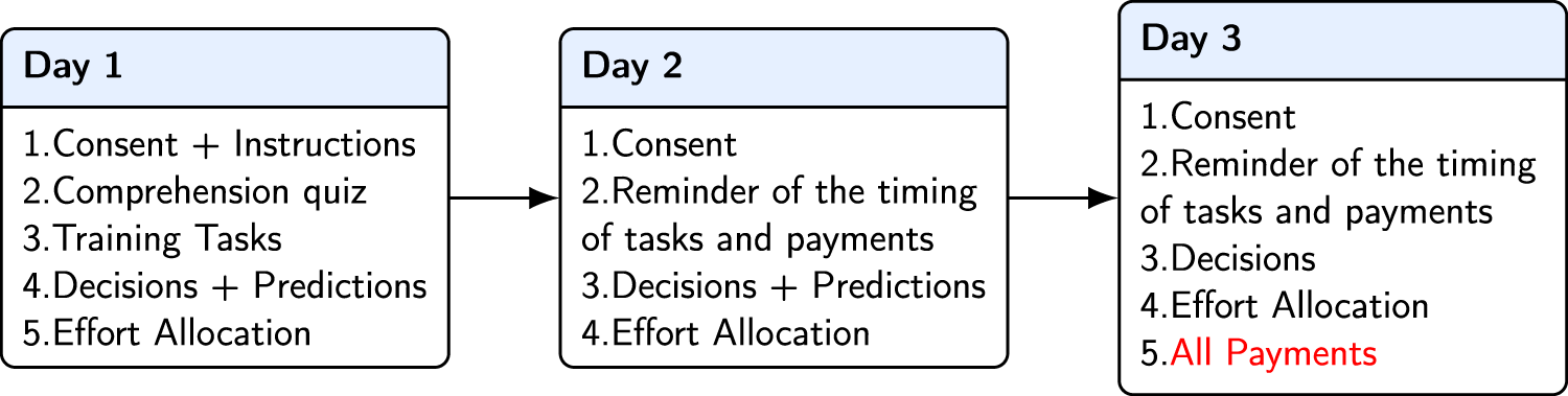





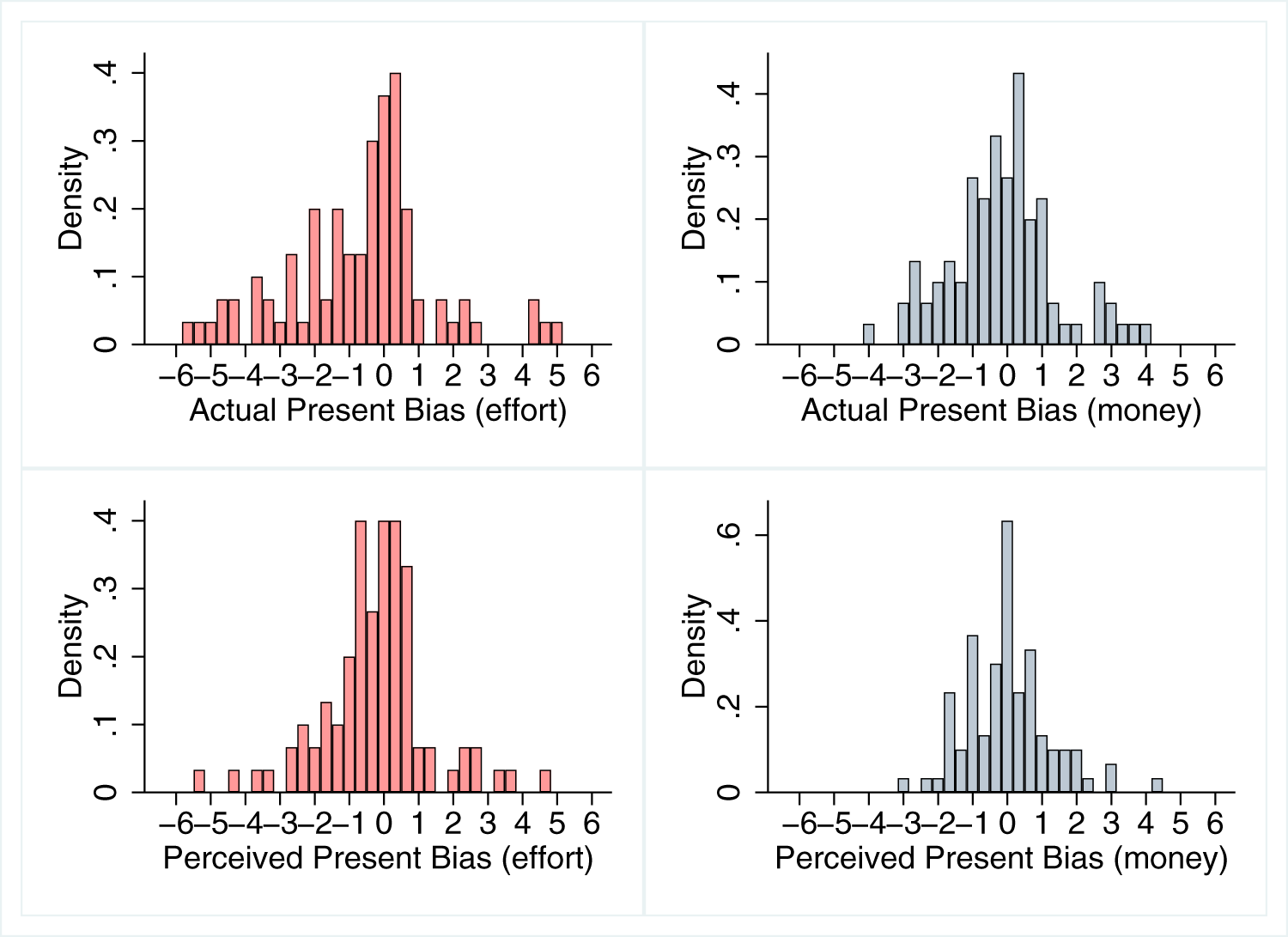


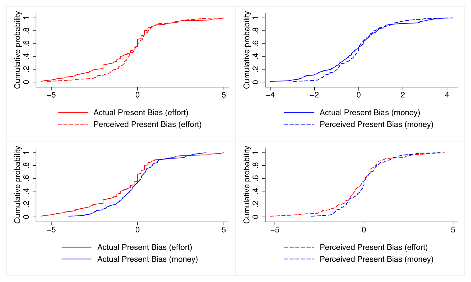


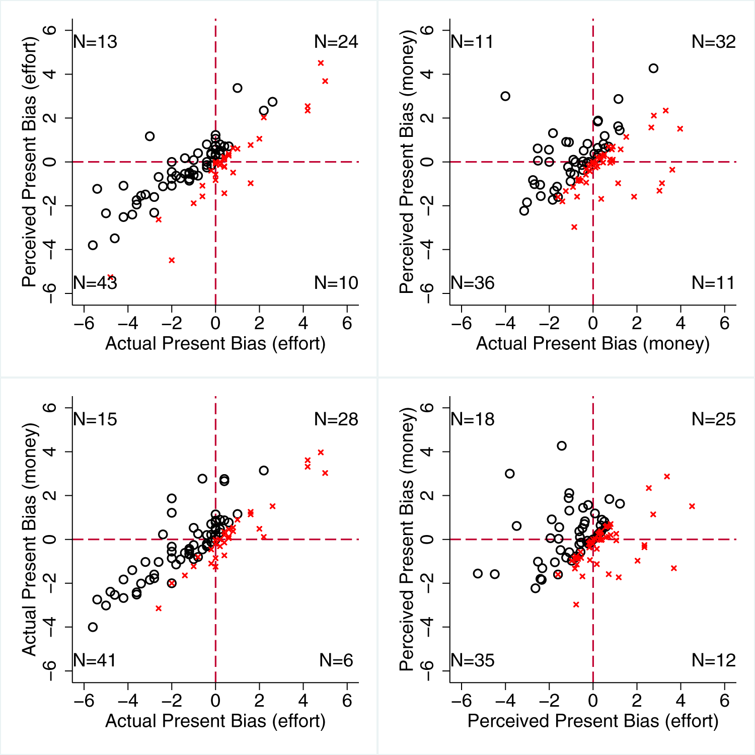
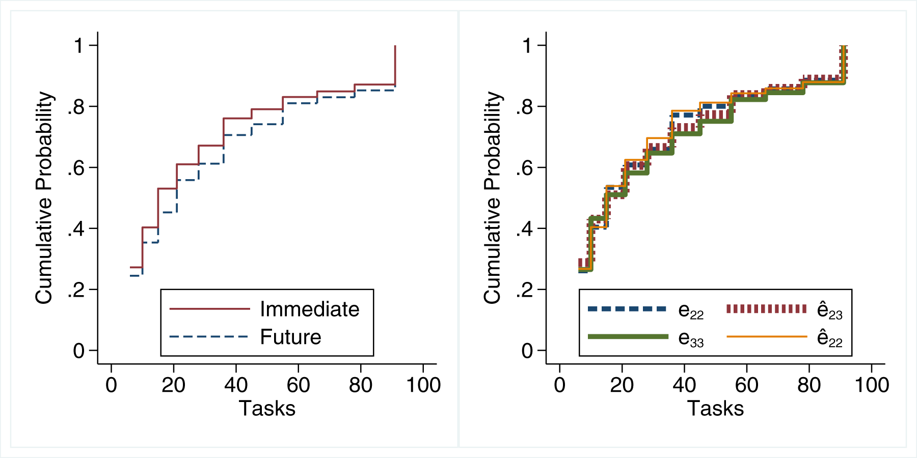


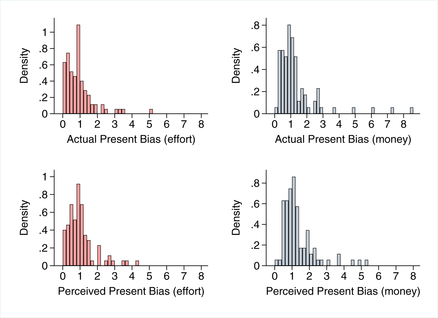
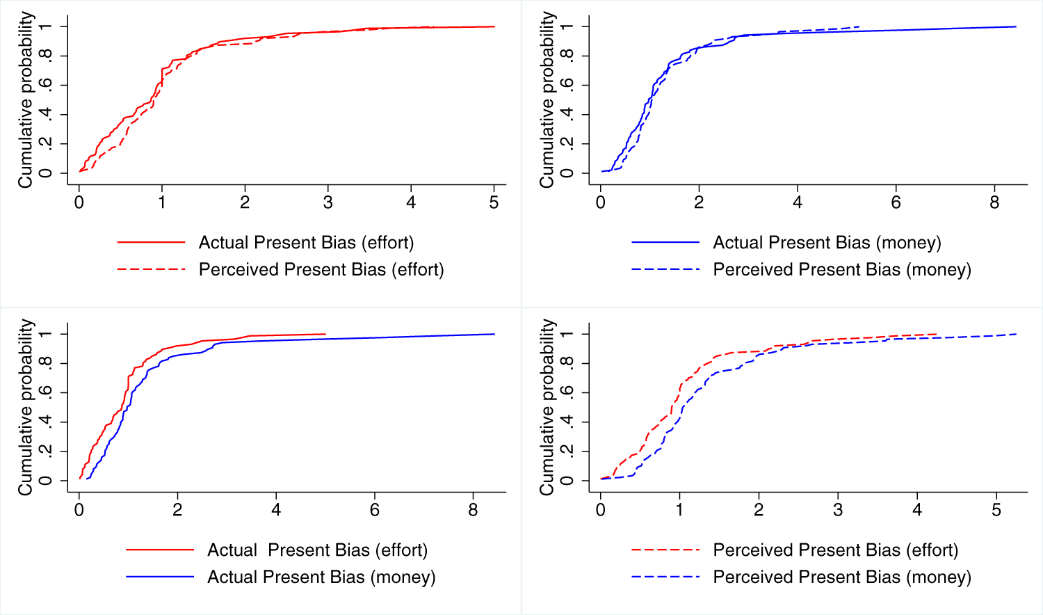


 Open access

