





Plain language summary
This article presents a method for recovering and comparing story trajectory curves. It draws on sentence embeddings, an extension of word embeddings, which represent words as points in a geometric space such that similarities in word meaning are denoted by similarities in geometric position. Contemporary embedding models, called “contextual embeddings” or “transformer embeddings”, can represent full sequences according to proximity in meaning and differentiate between distinct meanings and uses of the same words (polysemy). We use contextual sentence embeddings to represent 2,965 texts from Project Gutenberg fiction, concentrated primarily on the nineteenth century but ranging from the 1500s to the early 1900s. To do this, we divide or “chunk” each book into 128-token units, represent these chunks using contextual sentence embeddings, and structure them into sequences. We then apply a technique regularly used in the literature to construct “axes” representing binary oppositions as continua (in our case gender, class, morality, collectivity/individual, nature/artifice, order/disorder, and emotional/rational) and measure the relative position of each text chunk along these “axes.” This allows us to trace representational shifts along binary oppositions over the course of a book’s narrative sequence. We compute average sequences across all books and segment them by decade, genre, and dialogue speaker gender. Our analysis finds clear trends for each segment, many of which confirm ideas from narratological theory. While word embeddings have been used in historical language analysis, for example, to trace how words change over time periods, their use in representing books as chunked sequences is less common and builds upon work in book plot arc modeling with techniques like sentiment analysis. Our method is statistically robust and provides a proof of concept for how to analyze texts individually and in aggregate as sequences of embeddings.
Introduction
Narratology developed as the application of structuralist theory to narrative analysis, with a specific and somewhat unusual focus relative to structuralism in general on temporality. Specifically, narratology treats time as conditional, approaching a physical, given temporal sequence of events as independent and separable from its contingent, descriptive rendering in narrative order.
In natural language processing, word embeddings, perhaps more than any other recent technique, are conceptually affiliated with structural linguistics (Lenci and Sahlgren Reference Lenci and Sahlgren2023). Operationalizing embedding models for the analysis of text sequences has proven challenging, although recent transformer embedding models such as sentence-BERT make this tractable.
In this article, we present a proof-of-concept framework for the analysis of embedded literary sequences. Using a dataset of nearly 3,000 fiction books from Project Gutenberg, we represent books as sequence trajectories by embedding fixed text chunks with a sentence transformer model and then projecting chunks onto seven predefined semantic axes. We then aggregate individual text sequence trajectories into composite, mean trajectories to segment by variables such as time period, genre, or author/speaker gender.
Although the use of embeddings for time-series analysis is becoming increasingly common in multimodal embedding applications, analyzing temporal sequences with embeddings at the level of the text rather than the corpus is relatively less common, although it has been done before with success (Toubia, Berger, and Eliashberg Reference Antoniak and Mimno2021). Sequence analysis using embeddings has multiple advantages, however, for studying narratology: (1) it enables comparisons between the structural corpus level and the level of the individual text and (2) it enables the recovery of semantic patterns of temporal ordering and movement rather than static semantic associations. At the same time, ensuring that trajectories of embeddings are statistically real effects distinct from random noise, especially in aggregate, is a key challenge in any sequential embedding analysis.
In this article, we present our approach to the analysis of sequence semantics with transformer embeddings. We outline the method and evaluate its robustness, and then we apply it to the study of several corpus-level variables. We find that the approach accurately captures known genre and period-specific effects and that statistically it is highly robust compared to null comparison models. We conclude by suggesting that this method shows promise for the analysis of narrative sequences in general. (This includes narrative as broadly construed in the social sciences and humanities, and one could imagine extending this pipeline to corpora of documents, scientific articles, speeches, etc.)
Adapting word embeddings to narratology
Word embedding models such as word2vec (Mikolov et al. Reference Mikolov, Chen, Corrado and Dean2013) have been used widely in computational linguistics and social science to quantify and measure semantics. Word2vec originally emerged as an interpretive adaptation of historically “black box” neural network language models trained to predict sequences. Word2vec learned a high-dimensional geometric representation of the word (token) distribution such that semantically similar words mapped onto geometrically similar vector positions (as measured using dot product). Embedding models were trained by iteratively sampling the token co-occurrence distribution (i.e., the words that most frequently co-occur when sampling from large corpora) and solving for an optimal vector parameterization grounded in these corpus-wide token co-occurrence relations. In practice, this allows for measuring word similarity using geometric measures like cosine similarity and was famously shown to solve analogies with simple arithmetic, for example, king + (woman
$-$
 man) = queen.
Word embeddings are usually theorized in terms of distributional semantics (Lenci and Sahlgren Reference Lenci and Sahlgren2023), and this literature generally highlights overlaps between contemporary distributional models and structural linguistics, focusing on early linguistics analysis in American structuralism, by, for example, Zellig Harris and Leonard Bloomfield, who defined word similarity as a statistical measure of word co-occurrence frequency (Lenci and Sahlgren Reference Lenci and Sahlgren2023). Follow-up work using word embeddings and inspired by structuralism demonstrated the ability to recover subspaces or “semantic axes” from embedding representations by subtracting the average of vectors corresponding to binary oppositions (e.g., {good, ethical, moral} – {bad, unethical, immoral}). This was used to construct a direction in vector space between contrasting concepts and then measure arbitrary word positions along it (An, Kwak, and Ahn Reference An, Kwak and Ahn2018; Bolukbasi et al. Reference Bolukbasi, Chang, Zou, Saligrama and Kalai2016; Caliskan, Bryson, and Narayanan Reference Caliskan, Bryson and Narayanan2017; Ethayarajh, Duvenaud, and Hirst Reference Ethayarajh, Duvenaud and Hirst2019 ; Kozlowski, Taddy, and Evans Reference Kozlowski, Taddy and Evans2019). This approach, usually called “semantic axis projection,” has been used frequently both to measure intrinsic model bias on properties like gender as well as to measure sociolinguistic variation for properties like gender, class, or stereotypes in language data. Embeddings have also been applied (Garg et al. Reference Garg, Schiebinger, Jurafsky and Zou2018; Kozlowski, Taddy, and Evans Reference Kozlowski, Taddy and Evans2019) and extended (Charlesworth, Caliskan, and Banaji Reference Charlesworth, Caliskan and Banaji2022; Hamilton, Leskovec, and Jurafsky Reference Hamilton, Leskovec and Jurafsky2016) to the study of diachronic language change. These applications of word2vec to linguistic analysis focus on broad structural associations and diachronic shifts in large corpora. In many cases, they explicitly assume a structuralist orientation, tracing binary oppositions with semantic axis analysis in order to measure, for example, gender or class coding within corpora like Google Books (Charlesworth, Caliskan, and Banaji Reference Charlesworth, Caliskan and Banaji2022; Kozlowski, Taddy, and Evans Reference Kozlowski, Taddy and Evans2019).
It has been more challenging to extend word embedding models to the study of narrative. This is partly because narrative is highly focused on issues of structure and temporality that work at the level of the individual text rather than the corpus. Narratological theory, classical and postclassical, offers many and plural conceptualizations of narrative, but generally acknowledges that narratology involves the analysis of variability in how texts modulate formal properties, such as time, space, speaker position, or causation in order to represent events. In other words, narratives treat as conditional the kinds of mediating properties that would render the ordering of events into sequences an aesthetic construction rather than a natural and inevitable act.
This places the level of analysis in narratology somewhere between corpus structure and individual text, since it emphasizes how the formal sequencing of narrated content exhibits variation in the individual text that is also expected to adhere to broad intertextual patterns that emerge structurally in aggregate. If we conceptualize narrative this way, computational and statistical analysis would seem to have a place in narratology – provided that it can be operationalized to structure and analyze sequence over two temporal scales: the individual narrative sequence and the aggregate corpus sequence.
Most time-series analysis with word embeddings has focused on the aggregate corpus, as in the study of diachronic change in large corpora (e.g., to trace shifts in word usage over 100–200 years at the scale of Google Books). Static embeddings like word2vec generally struggle to embed time series at the scale of individual books, since the model is tuned for analyzing words in isolation rather than identifying how words come to assume distinct meanings in sequence context. Attempts to study individual text sequences by contrast have often drawn on methods like sentiment analysis on chunked sequence text (Jockers and Thalken Reference Jockers and Thalken2020; Öhman et al. Reference Öhman, Bizzoni, Moreira and Nielbo2024; Reagan et al. Reference Reagan, Mitchell, Kiley, Danforth and Dodds2016), LDA topic modeling (Elsner Reference Elsner2015), or tf-idf keyword analysis on trajectories (Boyd, Blackburn, and Pennebaker Reference Boyd, Blackburn and Pennebaker2020). Newer multimodal models like CLIP embed individual videos as time series and allow prompt-based retrieval with cosine similarity (Radford et al. Reference Radford, Kim, Hallacy, Ramesh, Goh, Agarwal, Sastry, Askell, Mishkin, Clark, Krueger and Sutskever2021). By contrast, there have been few comparable demonstrations to date of sequence analysis with word embeddings, although prior work that has tried this has been highly effective (Toubia, Berger, and Eliashberg Reference Toubia, Berger and Eliashberg2021). Part of the challenge with representing texts as sequences stems from the historical difficulty of modeling linguistic usage in sequence with static embeddings like word2vec – however this limitation has been ameliorated some in recent years with “contextual embeddings” (also called “transformer embeddings” to denote their use of the transformer architecture). Modern contextual embeddings using transformer language models like BERT (Devlin et al. Reference Devlin, Chang, Lee and Toutanova2019) and sentence-BERT (Reimers and Gurevych Reference Reimers and Gurevych2019) are specifically designed to disambiguate word meaning in sequence context.Footnote 1 This allows them to differentiate between the meaning of polysemous usages like ‘river bank’ versus ‘financial bank’. It also allows them to infer word reference, such as the antecedent to whom the word “they” refers in a given sequence context. Recent work has demonstrated the extensibility of existing word embedding techniques to contextual models. Lucy, Tadimeti, and Bamman (Reference Lucy, Tadimeti and Bamman2022) and Lucy and Bamman (Reference Lucy and Bamman2021) for instance recently demonstrated the applicability of familiar techniques used in static word embedding models such as word2vec, including semantic axis analysis and clustering, to the contextual embedding model BERT. There is also precedent for narratological analysis with contextual embedding models. Al-Laith et al. (Reference Al-Laith, Hershcovich, Bjerring-Hansen, Parby, Conroy and Tangherlini2024), for instance, used BERT as a classifier to identify binary distinctions related to noise in textual sequences, and Rockmore et al. (Reference Rockmore, Chen, Jebelli, Riddell and Stropkay2025) compared transformer contextual embeddings to tf-idf and other benchmarks in the context of literary text analysis. We explore here whether it is possible to adapt techniques for contextual embeddings to narrative analysis by modeling individual and aggregate text sequences in tandem. Our analyses are generally presented as proof-of-concept prototypes rather than fully developed evaluations, with the goal that they help establish the value and efficacy of sequence embedding analysis for future work.
Modeling sequences
Contextual embeddings such as sentence-BERT can effectively represent language at the two scales relevant to narrative: that of the individual text and that of the broader corpus. We suggest that this makes them specifically tailored to computational narratology. However, whereas measuring corpus-wide semantic associations and historical shifts has been well validated with static embedding models, representing text sequences with embeddings remains an emerging task in natural language processing.
To analyze how narratives are structured as temporal objects, we construct book sequence trajectory representations with embeddings derived from a pretrained sentence transformer model, which produces a single curve for each book in the corpus that we can then aggregate into pooled curve shapes and analyze along segments such as genre or decade. To do this, we start by chunking nearly 3,000 Project Gutenberg fictional texts into fixed 128-token segments and embedding each chunk with sentence embeddings. These yield book-level sequence representations. This allows us to apply embedding techniques like semantic axis analysis to textual sequences at the scale of individual books, exploring how various constructs vary throughout a text’s narrative structure. Throughout, we measure seven semantic axes applied to each individual chunk: gender, class, morality, collectivity/individual, nature/artifice, emotional/rational, and order/disorder.
We then compile these projections into curves by resampling book sequences to the same normalized length and applying Gaussian smoothing to recover macro-level semantic patterns. We then pool these representations into aggregated curve shapes to further study how various subsets of the corpus such as genre, decade, or author gender tend to represent sequence in patterned forms. Since our approach relies on a somewhat new unit of analysis – embedded sequence segments – we outline our approach in more detail in this section and report several steps to validate its robustness prior to presenting the results.
Corpus acquisition and preprocessing
We use the gutenberg
$\!\!\_$
 english repository on HuggingFace’s datasets repository, which covers over 80 percent of all English books on Project Gutenberg. We load the first 4,000 texts, representing slightly under 10 percent of the dataset (48,284 books total). We then filter within the metadata to members of the fiction category, yielding 2,965 texts. To do this, we extract “bookshelves” or “subjects” containing any of the keywords “fiction,” “novel,” “story,” “drama,” or “poet.” This represents about 6 percent of the overall dataset, or around
$>4.8$
english repository on HuggingFace’s datasets repository, which covers over 80 percent of all English books on Project Gutenberg. We load the first 4,000 texts, representing slightly under 10 percent of the dataset (48,284 books total). We then filter within the metadata to members of the fiction category, yielding 2,965 texts. To do this, we extract “bookshelves” or “subjects” containing any of the keywords “fiction,” “novel,” “story,” “drama,” or “poet.” This represents about 6 percent of the overall dataset, or around
$>4.8$
 percent of all of Gutenberg’s English fiction texts. A small number of nonfiction false positives appear to fall through but are rare and likely Gutenberg metadata labeling issues; this likely introduces some noise, but it also makes the fiction estimates conservative. Project Gutenberg also includes “complete works” and multivolume editions of texts, which could introduce some additional sequence noise. We estimate book year by extracting from metadata, whenever available, the author’s birth year, which roughly designates relative authorship time periods for books when comparing between rather than within authors.
We next embed each book in full using the HuggingFace sentence transformer model all MiniLM L6 v2 and use the final layer for analysis, as is conventional. We embed chunks of 128 tokens to encode individual books as sequences of embeddings. We leave unit score normalization off initially but normalize later when projecting axes using cosine similarity.
Constructing semantic axes
Semantic axis analysis is performed trivially with word2vec by measuring word cosine similarity to a direction vector usually defined by subtracting the mean of semantically opposite token vectors, for example, {good, ethical, moral} – {bad, unethical, immoral}. With contextual embeddings, single token subtractions tend to yield unstable axes, since contextual embeddings vary embedding position by surrounding sequence context, meaning that a given token like “good” will not inherently map onto its mean corpus usage. There is limited albeit emerging consensus on how best to operationalize semantic axes for contextual embeddings. Some studies use single words, or simple phrase templates, with the recognition of the potential for axis instability. Lucy et al. (Reference Lucy, Tadimeti and Bamman2022) propose subtracting the means of numerous sampled contextual examples of word opposition pairs, drawing from, for example, the Wikipedia corpus (which maintains independence from their focal study corpora). Recent work applying sentence transformers such as Zeng et al. (Reference Zeng, Jin and Voigt2024) uses wordnet derived antonym pairs to construct initial semantic axes that are pruned with LLM assistance, then later projects masked contextual samples for numerous example texts about various groups onto them to measure how the axis position varies for the contexts surrounding the masked words denoting the group. In our case, fiction books, using Wikipedia sampling such as in Lucy et al. (Reference Lucy, Tadimeti and Bamman2022) is less directly applicable since word usage varies considerably between nineteenth century fiction and contemporary encyclopedia form.
One alternative to single token representations or Wikipedia sampling is to sample tokens over many contexts within the Project Gutenberg corpus itself. Although this risks some possible circularity since we are measuring the same texts used to define the axes, it is also more likely to capture historically specific semantics than if we were to draw on contemporary corpora. As a robustness evaluation, we construct axes from (a) individual word token oppositions and (b) random context samples from our Project Gutenberg corpus. We then compare axis similarities to test how closely they align. For the seven contextual semantic axes, we randomly sample the Gutenberg fiction corpus for up to 10,000 contextual examplesFootnote 2 for each of the following individual seed words, then construct axis poles from the unit score normalized embedding means of those contextual samples. We then subtract these poles to compute the semantic axes. We report seed terms in Table 1.Footnote 3
Axis seed words
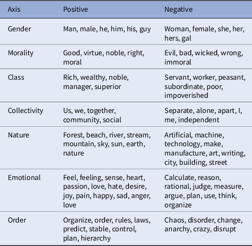
Table 1 Long description
The table consists of three columns: Axis, Positive, and Negative.
1. Gender: Positive includes Man, male, he, him, his, guy. Negative includes Woman, female, she, her, hers, gal.
2. Morality: Positive includes Good, virtue, noble, right, moral. Negative includes Evil, bad, wicked, wrong, immoral.
3. Class: Positive includes Rich, wealthy, noble, manager, superior. Negative includes Servant, worker, peasant, subordinate, poor, impoverished.
4. Collectivity: Positive includes Us, we, together, community, social. Negative includes Separate, alone, apart, I, me, independent.
5. Nature: Positive includes Forest, beach, river, stream, mountain, sky, sun, earth, nature. Negative includes Artificial, machine, technology, make, manufacture, art, writing, city, building, street.
6. Emotional: Positive includes Feel, feeling, sense, heart, passion, love, hate, desire, joy, pain, happy, sad, anger, love. Negative includes Calculate, reason, rational, judge, measure, argue, plan, use, think, organize.
7. Order: Positive includes Organize, order, rules, laws, predict, stable, control, plan, hierarchy. Negative includes Chaos, disorder, change, anarchy, crazy, disrupt.
As noted, we construct axes from seed terms only versus from 10,000 per-term contextual examples and report the comparison in Table 2.
Single token versus Gutenberg fiction contextual axis comparison
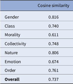
Table 2 Long description
The table consists of two columns: the first lists the contextual axis category and the second lists the corresponding Cosine similarity value.
* Gender: 0.816
* Class: 0.740
* Morality: 0.611
* Collectivity: 0.748
* Nature: 0.806
* Emotion: 0.674
* Order: 0.761
* Overall: 0.737
Contextual sampling from our corpus is modestly similar (0.737 cosine similarity) to single token subtractions, suggesting that the two capture relatively similar semantics, though there is some variation across the seven axes. Given that the two approaches appear generally comparable and since contextual axes are theoretically motivated, we elect to use Gutenberg context sampling for axis construction in the main analysis.
We next validate the axis out of sample on a set of 420 curated antonym pair sentences, scaled with assistance from GPT-5. We present these results in Table 3.
Axis validation for 420 out-of-sample manually crafted antonym sentence pairs
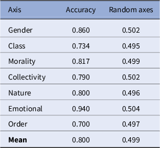
Table 3 Long description
The table consists of three columns: Axis, Accuracy, and Random axes.
Row 1: Gender axis has an accuracy of 0.860 and random axes value of 0.502.
Row 2: Class axis has an accuracy of 0.734 and random axes value of 0.495.
Row 3: Morality axis has an accuracy of 0.817 and random axes value of 0.499.
Row 4: Collectivity axis has an accuracy of 0.790 and random axes value of 0.502.
Row 5: Nature axis has an accuracy of 0.800 and random axes value of 0.496.
Row 6: Emotional axis has an accuracy of 0.940 and random axes value of 0.504.
Row 7: Order axis has an accuracy of 0.700 and random axes value of 0.497.
Row 8: The Mean across all categories is 0.800 for accuracy and 0.499 for random axes.
These results are out-of-sample validations tested on contemporary examples, not historical Gutenberg fiction. Accuracy is based on whether the axis projection polarity (measured by its sign value) matches the labeled polarity (e.g., individualist vs. collective) for each sentence. Accuracies in all cases exceed 0.700 and are 0.800 on average. Despite using fixed linear projections rather than trained classification, accuracies are comparable to simple supervised baselines. We additionally compare to random null axes, which we expect to predict validation pairs at random chance. Across 1,000 random unit length axes per dimension, none approach the performance of the constructed axes. We compared these axes to the single-token derived seed axes as well and found comparable performance on this validation task (mean = 0.820). We report some of the top scoring sample chunks for face validity in Table 4.
Examples of top scoring chunks by axis for each pole
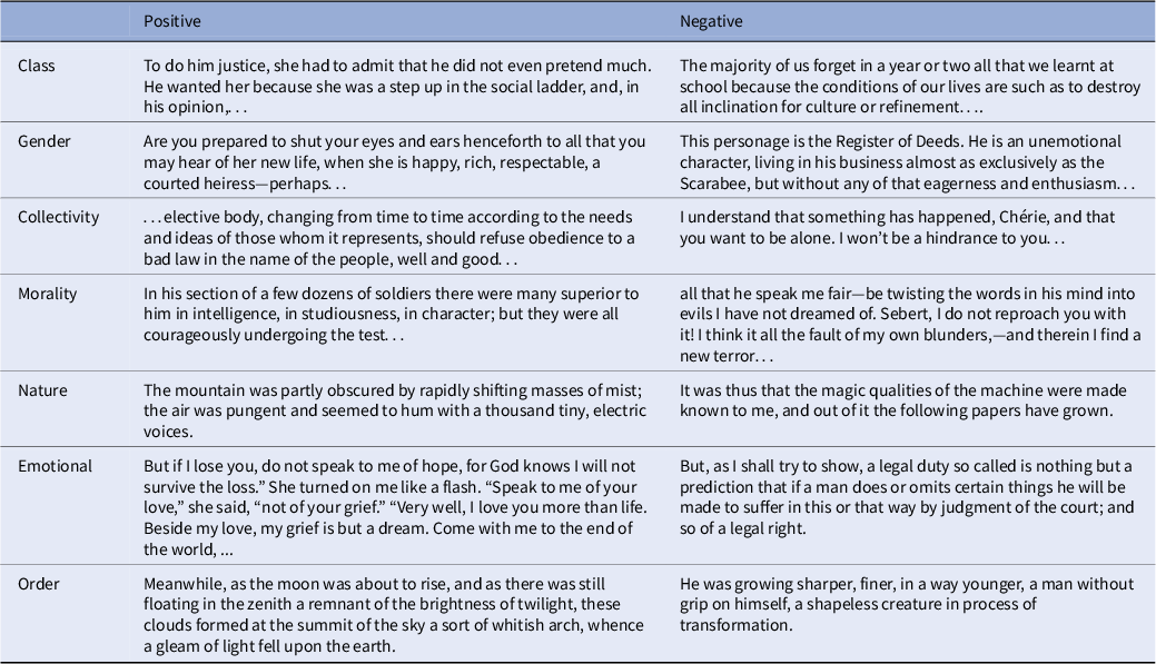
Table 4 Long description
The table consists of three columns: Axis (unlabeled header), Positive, and Negative.
1. Class: The Positive excerpt describes a woman admitting a man wants her for social advancement. The Negative excerpt discusses forgetting school lessons due to life conditions destroying culture.
2. Gender: The Positive excerpt asks about ignoring a woman's new respectable life. The Negative excerpt describes a Register of Deeds as an unemotional character.
3. Collectivity: The Positive excerpt discusses an elective body refusing bad laws in the name of the people. The Negative excerpt features a character named chérie wanting to be alone.
4. Morality: The Positive excerpt describes soldiers superior in character undergoing a test. The Negative excerpt involves a character named Sebert and a fear of twisted words and blunders.
5. Nature: The Positive excerpt describes a mountain obscured by mist and pungent air. The Negative excerpt mentions the magic qualities of a machine.
6. Emotional: The Positive excerpt is a dialogue about love being more important than grief. The Negative excerpt defines legal duty as a prediction of suffering by court judgment.
7. Order: The Positive excerpt describes a whitish arch of clouds and moonlight. The Negative excerpt describes a man becoming a shapeless creature without self-grip.
Following Antoniak and Mimno (Reference Antoniak and Mimno2021) who show that semantic axes are fragile to seed word selection, we also evaluate robustness to seed choice. We perform single token leave-one-out ablations for our contextual axis to evaluate robustness to seed term selection. Cosine similarities to the original axis are consistently high (cosine similarity 0.90) across all terms and axes. We report full results in the Supplementary Material. We also compare cosine similarities for each axis to placebo axes, which randomly reorder tokens, in Table 5.
Comparison to placebo axes
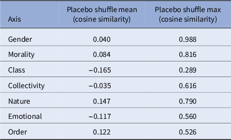
Table 5. Long description
The table consists of three columns: Axis, Placebo shuffle mean (cosine similarity), and Placebo shuffle max (cosine similarity).
* Gender: mean 0.040, max 0.988.
* Morality: mean 0.084, max 0.816.
* Class: mean minus 0.165, max 0.289.
* Collectivity: mean minus 0.035, max 0.616.
* Nature: mean 0.147, max 0.790.
* Emotional: mean minus 0.117, max 0.560.
* Order: mean 0.122, max 0.526.
Constructing semantic sequence curves
We next analyze chunked semantic axis projection sequences as sequence curve plots. To do this, we normalize books of varying lengths to the same length through resampling, then apply smoothing to recover macroscopic trends. We then pool curves into aggregated trajectory plots. We describe the procedure below, then report a set of robustness tests. Composite embedded sequences are a somewhat new artifact – while embedded sentences and time-series embeddings are sometimes analyzed, whether broad axis projection patterns at the scale of the book are statistically meaningful is an open question. We statistically test against a time-shuffled null model below, and we also statistically evaluate the robustness of various smoothing and resampling parameter selections; in all cases, we find strong statistical robustness. We additionally briefly compare our model to sentiment analysis and keyword-based trajectories, which have also been used in the literature to construct narrative curves. These results are presented in the remainder of this section.
First, however, we briefly discuss the theoretical validity of our approach. Our aim is to present a preliminary proof-of-concept method for analyzing embeddings at the level of book-length sequences. Our sequence curves are meant as minimal, parsimonious representations of semantic trajectories rather than definitive narrative arc shapes, which is why we limit processing to resampling and smoothing. This method is intended to recover statistical tendencies rather than definite forms, like the “six archetypal story narratives.” Nevertheless, we do make a somewhat strong assumption that semantic tendencies at the scale of individual texts can aggregate into pooled sequences that reveal meaningful intertextual trends in semantic sequencing. Although we test this assumption statistically below, conceptually, it adheres to a genre-theoretic interpretation that intertextuality derives not only from borrowing a shared repertoire of topics, but also from a) sequencing them along shared temporal orderings and b) constructing them using shared, corpus-level structural binary oppositions. In other words, our statistical model is intentionally lightweight, which is intended to allow us to empirically test long-articulated but comparably stronger theoretical assumptions from narrative and structuralist theory.
Plotting procedure
For plotting embedded sequences as normalized and aggregated curves, we resample and smooth the raw embedding projection score sequences then plot pooled composite curves. We first resample chunked sequences to 300 time points by linearly interpolating between points and then sampling equally along the interpolated curve. Resampling normalizes books of distinct lengths, allowing us to compare books on the same time scale. Conceptually, resampling normalizes books of differing lengths onto the same time scale by interpolating lines between neighboring points and sampling equally along the interpolated curve. In many cases, when resampling to 300 time units with 128-token chunks, this will downsample longer books onto a shortened normalized time scale with lower resolution. We considered alternative forms of interpolation, as well as non-interpolated alternatives, such as taking the means of standard buckets, but found linear interpolation to preserve the most signal while maintaining the simplest set of assumptions.
We then apply Gaussian smoothing to focus on the most salient trends and reduce noise. Smoothing functions like a low-pass filter that dampens the highest frequencies – often noisy local fluctuations – to recover slower moving trends comprising the underlying global curve shape. Bootstrapping with 95th confidence intervals was applied to plots when noted. Plots show axis similarities using cosine similarity except where they also use z-scoring when noted. Z-scoring removes the absolute scale and plots axis motion per chunk along a standard scale. We do not use it when trying to show variations in semantic axis value means or amplitudes. To construct aggregate mean trajectory plots, we average the projection scores for each chunk to compute a composite curve.
Time-shuffled null comparison
It is possible that averaging semantic axis projection trajectories across many books might result in curves that appear qualitatively meaningful but are indistinct from patterns that emerge by random chance. To test whether our aggregate curve shapes are different from random distributions, we compare to a within-book time shuffle null, which randomly permutes chunk order within books while maintaining the semantic axis projection values of the permuted chunks (Figure 1). This evaluates the degree to which the temporal sequence order of projection values makes a meaningful difference to the recovery of curve shapes. The observed aggregate curves are dramatically more structured than within-book shuffle null curves. For instance, the observed range exceeds the median null range by more than an order of magnitude on every axis, all of which are statistically significant at
$p < 0.001$
 (e.g., morality: 2.54 vs. 0.013; class: 1.60 vs. 0.013; and emotional: 1.52 vs. 0.013).
Observed z-scored corpus-level mean trajectories (black) compared with a within-book time shuffle null (gray), obtained by randomly permuting chunk order within each book while preserving the set of chunk-level semantic axis projection values. Shaded bands show the central 95 percent of shuffled aggregate curves. Across all axes, observed trajectories have substantially larger temporal range than the shuffled null trajectories (
$p<0.001$
 ), indicating that the observed trajectories depend on narrative ordering rather than semantic composition only.
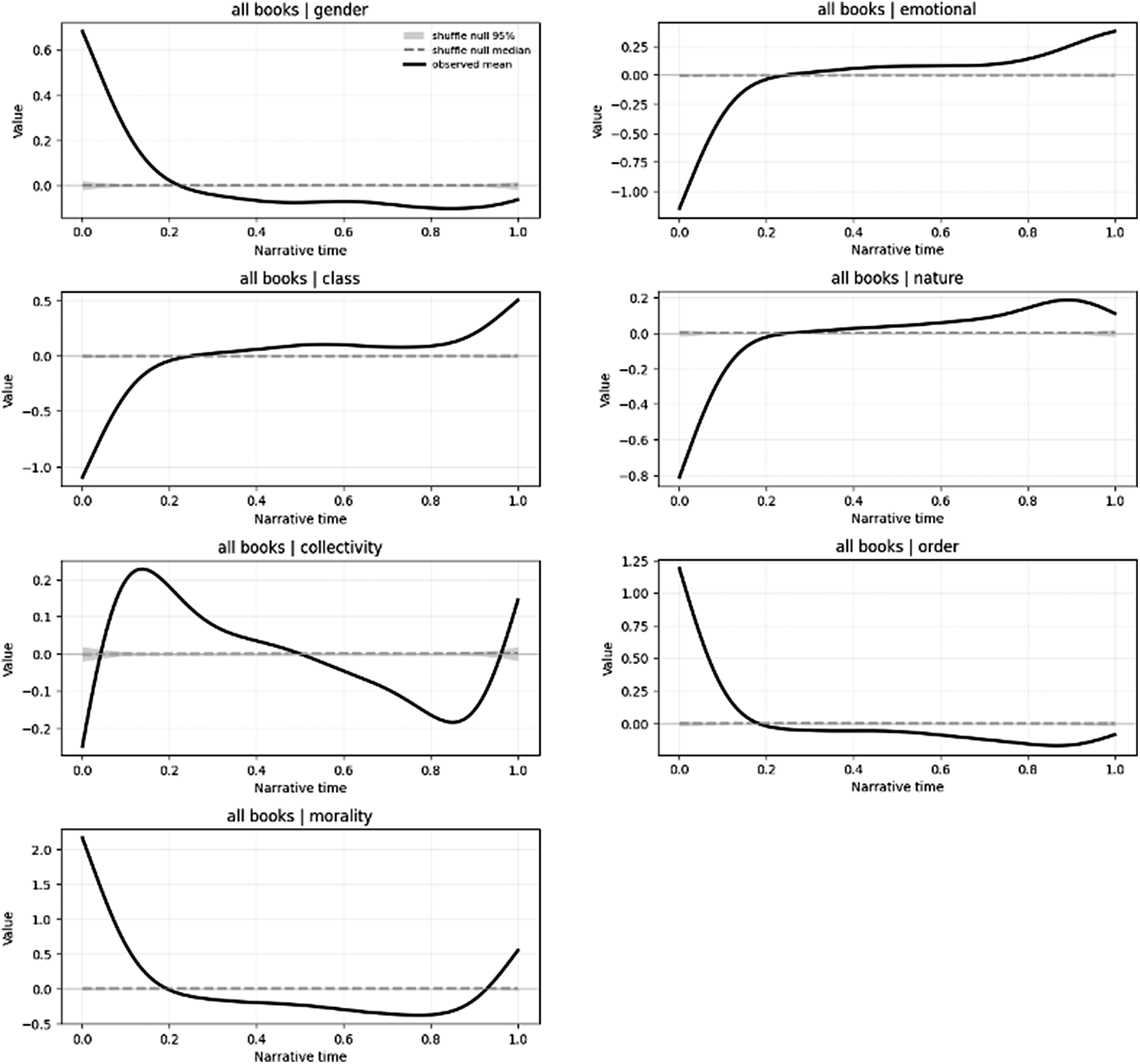
Figure 1 Long description
The figure consists of seven line graphs arranged in a two-column grid. Each graph shares the same axes: the x-axis is Narrative time from 0.0 to 1.0, and the y-axis is Value. A legend in the first panel identifies three components: a solid black line for observed mean, a dashed gray line for shuffle null median, and a light gray shaded band for shuffle null 95 percent. In all panels, the shuffle null remains flat at zero, while the observed mean shows significant fluctuation.
* Top-left, all books | gender: The curve starts high at 0.7, drops sharply to cross zero at 0.2, and remains slightly negative through the end.
* Top-right, all books | emotional: The curve starts very low at -1.1, rises steeply to cross zero at 0.2, and continues a gradual upward trend to 0.4.
* Second row left, all books | class: The curve starts at -1.1, rises to zero by 0.3, plateaus slightly, and then rises sharply at the end to 0.5.
* Second row right, all books | nature: The curve starts at -0.8, rises to zero by 0.2, peaks slightly at 0.2 around 0.9 narrative time, and ends at 0.1.
* Third row left, all books | collectivity: The curve starts at -0.25, peaks sharply at 0.23 around 0.15 time, crosses zero at 0.5, dips to -0.18 at 0.85 time, and rises to 0.15.
* Third row right, all books | order: The curve starts high at 1.2, drops to zero by 0.2, and stays slightly negative, ending at -0.1.
* Bottom-left, all books | morality: The curve starts at its highest point of 2.2, drops to zero by 0.2, reaches a trough of -0.4 at 0.75 time, and rises to 0.5 at the end.
Chunking and smoothing stability
Chunking stability: We embed chunked text; chunking the sequences splits it into equal text intervals. It does not attempt to isolate meaningful narrative “beats,” but simply samples on a consistent time unit. It is possible that shortening or lengthening chunk window sizes could influence semantic values. We evaluate the robustness of our results to chunk lengths of half (64 tokens) and twice (256 tokens) the size of our main text chunk window size on a reduced random subsample of 10 percent of the corpus and find strong overall median correlations to each (64 tokens = 0.920, 256 tokens = 0.934) and median correlation consistently greater than 0.90 across our seven semantic axes. We report full results in the Supplementary Material.
Smoothing stability: One significant potential threat to the validity of our analysis is the smoothing procedure. Smoothing is widely used in time-series analysis and necessary to produce interpretable curve forms, but it risks introducing structure not present in the data. To test for this, we check sensitivity to smoothing parameters by measuring Pearson’s correlation between various smoothing coefficients and chunk sizes against a reference sequence. We run these for the diachronic, genre, and gender analyses reported in the main results, testing smoothing factors of 0.00, 0.05, 0.10, and 0.15 and resampling sizes of 100, 240, and 500. We also evaluate null control results, by shuffling chunk order randomly within books, to tests whether sequence structure randomizes. While correlations with the raw sequences are moderate, as expected, correlations to even lightly smoothed curves are consistently above 0.90–0.95. Null results clearly randomize sequence structure, although they maintain absolute semantic offset, as expected. Smoothing qualitatively tracks raw sequence trends, and the analysis is robust to smoothing parameter variation overall. We find the same effects when testing by various variables, including decade, genre, and gender. It is unlikely that smoothing plays a substantial role in synthesizing or disrupting sequence trends. Full smoothing validation results are presented in the Supplementary Material.
Even given strong statistical results, we briefly justify our choice of smoothing and raise possible limitations. Smoothing chunked sequences acts as a low-pass filter dampening the signal’s highest frequency bands to recover the underlying curve shape. If we assume that rapid frequency changes are largely local effects, applying a low-pass filter to the sequence should extract genuine low-frequency curve structure if it exists rather than synthesize spurious patterns (unless the smoothing factor is extremely large). Conceptually, smoothing gives priority to long-term semantic trends over short term, reversible oscillations. Narratologically, curve smoothing assumes that thematic language, such as individual versus collective language, temporally repeats in a patterned way across several chunks even if local chunks show brief deviations – in other words, smoothing isolates moments where a semantic pattern is sustained for more than short-term intervals. However, narratives communicate not only through consistent repetitions but also through dialectical constructs (e.g., “I am far from the crowd”). Smoothing does not eliminate dialectical constructs if they persist over several chunks, but it means that we must interpret apparently neutral trends cautiously; a neutral trend does not necessarily indicate the absence of a binary opposition, but may also indicate the integration of opposites.
Comparison to sentiment analysis and tf-idf keywords
There are two opposing analytic risks with embedding sequences for narrative analysis: (1) that they fail to add additional information beyond existing methods, such as sentiment analysis or keyword counts and (2) that they are uninterpretable and fail to track existing sequence analysis techniques, such as sentiment analysis and keyword counts. To check robustness to both of these, we compare our embedded sequence projections to VADER sentiment scores on chunked sequences and to tf-idf keyword measures, per chunk, of the seed words used to construct our semantic axes. When comparing to sentiment analysis, we find moderate to strong correlations between VADER sentiment trajectories and all of our axes at the median. The highest correlations are to the collectivity (0.854), gender (0.706), nature (
$\!\!-$
 0.728), morality (0.686), and order (0.691) axes, with moderate correlations to the class (
$\!\!-$
0.728), morality (0.686), and order (0.691) axes, with moderate correlations to the class (
$\!\!-$
 0.459) and emotional (
$-$
0.459) and emotional (
$-$
 0.545) axes. These correlations reflect the fact that our axes are constructed through valenced oppositions that often embed evaluation. However, they are also potentially consistent with the possibility that many binary contrasts in nineteenth century fiction are structured through evaluative distinctions. The moderate to high correlations generally suggest that a substantial fraction of variance along most semantic axes aligns with valence, while the semantic axes further capture more specific semantic directions that are irreducible to overall sentiment. Conceptually, this potentially suggests, consistent with structural linguistics, that semantic axes show how narratives move through different “categories” of concepts that are each constructed in structurally valenced terms as relatively good or bad.
Our tf-idf keyword analysis shows small albeit modest correlation with all but the “order” axis (median class =
$-$
 0.296, collectivity = 0.279, emotional = 0.607, gender = 0.206, morality =
$-$
0.296, collectivity = 0.279, emotional = 0.607, gender = 0.206, morality =
$-$
 0.340, nature = 0.345, and order = 0.041), with the highest correlation with the “emotional” axis (0.607). This is expected since contextual embeddings measuring text projections onto semantic axes should be adding much more information than raw keyword counts, though it also suggests that contextual axes remain semantically grounded relative to a simpler baseline.
Analytic strategy
We briefly outline the set of analyses we perform in the following sections.Footnote 4 First, similar to Charlesworth, Caliskan, and Banaji (Reference Charlesworth, Caliskan and Banaji2022), Hamilton, Leskovec, and Jurafsky (Reference Hamilton, Leskovec and Jurafsky2016), Kozlowski, Taddy, and Evans (Reference Kozlowski, Taddy and Evans2019), or Al-Laith et al. (Reference Al-Laith, Hershcovich, Bjerring-Hansen, Parby, Conroy and Tangherlini2024), we report aggregate diachronic trends for the seven semantic axes by decade (although again here we differ in analyzing down-sampled mean narrative sequences per decade). We next visualize mean sequence axis projections by genre, to determine how genre modulates the same content categories through varying narrative form.
Following computational work from Jockers and Kirilloff (Reference Jockers and Kirilloff2016) and Jockers and Mimno (Reference Jockers and Mimno2013) on nineteenth century gendered novel representations, we next analyze the influence of author and character gender on our semantic narratological arcs. We label authors by gender using a simple names list from the Natural Language Toolkit (NLTK).Footnote 5 We then extract all dialogue quotations per book and check the speaker’s gender by scanning for name matches within a ±20-word windowFootnote 6 and labeling them by gender. This allows us to segment sequence semantic axis projections by author gender versus speaker gender, enabling us to trace patterns in the representations of gendered dialogue. (The purpose of this, described further in the next section, is to trace how character voice is constructed by standpoint and how this bears on sociolinguistic gender constructions in the emerging novel form, following arguments proposed by feminist postclassical narratological theory.)
Lastly, prior to presenting results, we briefly operationalize a provisional definition of narrative as we approach the construct here, as distinct from pure literary temporality. We earlier informally suggested that narrative involves the conditional ways in which a set of events can be mediated through, for example, temporal order, speaker position, awareness of the reader, or causal sequence. Prince (Reference Prince2019, Reference Prince2012) gives a parsimonious and formal definition: “A narrative is a verbal or non-verbal entity taken to constitute the representation of at least two related asynchronous events (or one state of affairs and one event) that do not presuppose or imply each other.” Prince is here defining narratives as a set of events (or event–state pairs) that are a) related through an ordering in time b) not simultaneous c) and not logically implied. By this Prince separates descriptions like “when I poured water to the top of the glass it was full” (not a narrative but a logical implication) or uncorrelated simultaneous incidents like “the sun set as the glass broke” from “related” sequences like “after I poured water in the glass, it broke” (Prince Reference Prince2012). So narrative by this definition is again the study of how meaning is encoded in ordered sequences. In other words, analyzing sequence is analyzing narrative – with the caveat that not all sequences are narrative sequences. Our method does not strongly endeavor to separate out narrative and non-narrative representations of time at the micro-level – for example, our sequence models are not filtering out chunked sequences using Prince’s criteria. At statistically large scales, however, when comparing across narrative forms (which all of our texts are), we suggest that many non-narrative utterances should be controlled out as randomly distributed, leaving intentional narrative construction explaining a non-trivial amount of the patterned variance. We also anticipate that non-narrative sequences (like logical entailment) should be more rare than narrative sequence. However, we briefly evaluate this assumption empirically in the Supplementary Material with a small classifier trained on positive and negative examples following Prince’s definition applied to a sample of the Gutenberg fiction corpus.
Finally, we provide a visual schematic diagram of our approach in Figure 2.
Schematic diagram of our approach to semantic trajectory embedding.
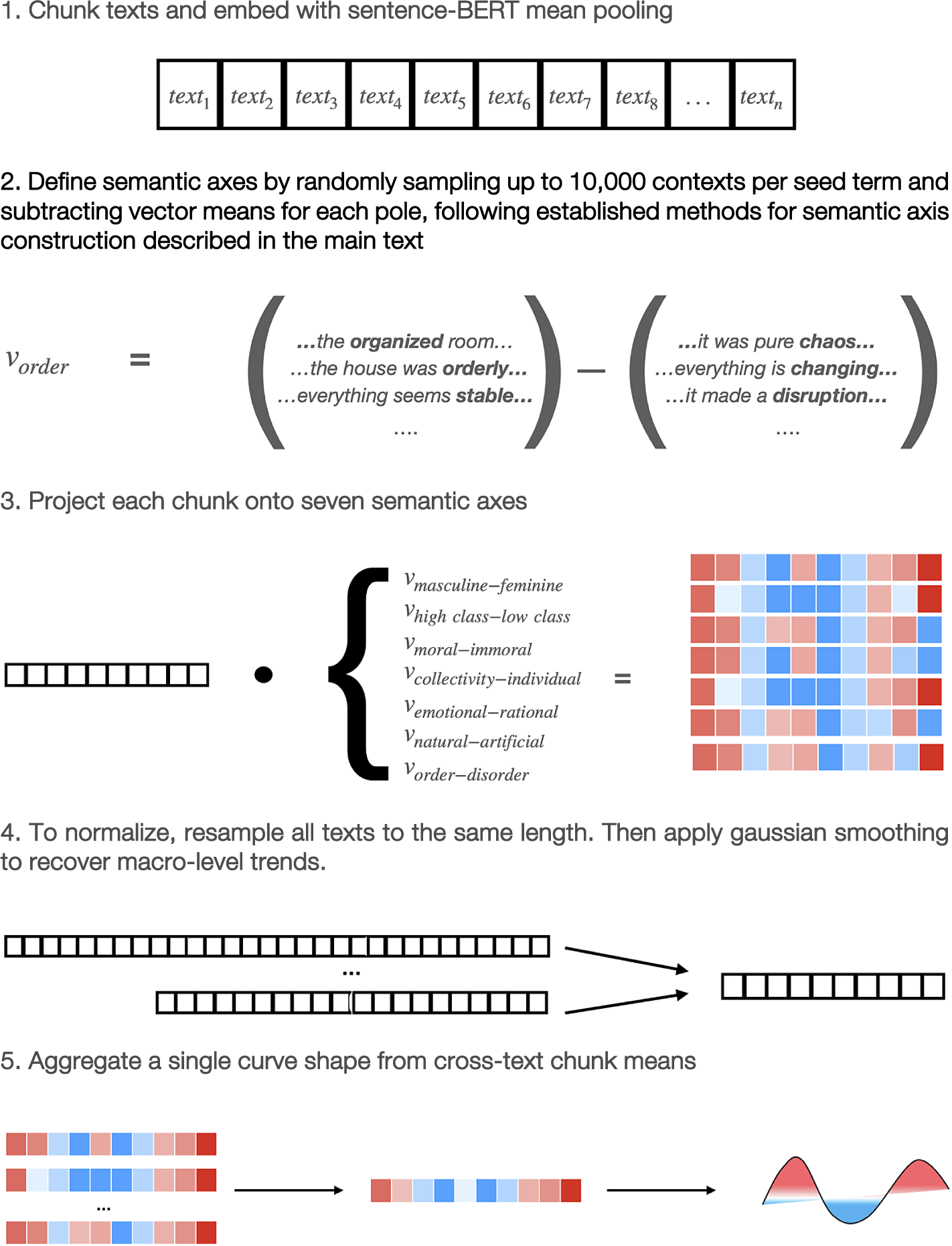
Figure 2 Long description
The diagram is organized into five sequential steps.
* Step 1. Chunk texts and embed with sentence-B E R T mean pooling. A horizontal row of boxes contains labels text sub 1, text sub 2, through text sub n.
* Step 2. Define semantic axes by randomly sampling up to 10,000 contexts per seed term and subtracting vector means for each pole. An equation shows V sub order equals the difference between two sets of parenthetical text examples. The first set includes phrases like organized room, orderly, and stable. The second set includes chaos, changing, and disruption.
* Step 3. Project each chunk onto seven semantic axes. A dot product operation is shown between a horizontal vector and a bracketed list of seven axes: V sub masculine-feminine, V sub high class-low class, V sub moral-immoral, V sub collectivity-individual, V sub emotional-rational, V sub natural-artificial, and V sub order-disorder. This results in a heatmap grid of red and blue squares.
* Step 4. To normalize sequences by book length, resample all texts to the same length, then apply Gaussian smoothing to recover macro-level trends. Two long horizontal vectors of different lengths point toward a single standardized vector.
* Step 5. Aggregate a single curve shape from cross-text chunk means. A stack of heatmaps is averaged into a single row of colored squares, which then transforms into a continuous wave-like line graph with red peaks and blue troughs.
Results
General diachronic trends
Generalizing, the rise of the novel has often been understood as concentrating around eighteenth century works focused on moral instruction that develop in the nineteenth century into early realist and increasingly individualist portrayals (Watt Reference Watt2001). Similarly, the broadly increasing entry of women writers into novel publication in the nineteenth century played a significant role in constituting the form. The period also coincides with a shift from Enlightenment era literature to Romantic era literature, highlighting nature, emotions, and the individual. Our modeling strategy allows us to test for the presence of these trends in the Gutenberg data, by observing changes in mean plot trajectory shape along our seven semantic axes by decade. These sequence trends when measured in aggregate are broad and general, but they align with widely observed shifts in narrative form occurring during this time period.
We observe in Figure 3 a matching, gradual shift over decades toward more individualist than collectivist, less moralizing, more natural than artificial, and more disordered rather than ordered language, along with a slightly less pronounced trend toward more emotional than rational language. This shift seems to match the general trend toward Romantic era themes (concerning emotions, nature, the individual, and a critique of order, reason, and conventional morality) and away from earlier Enlightenment era themes (more closely focused in this data on artifice, the collective, morality, order, and reason).
Diachronic change (1800–1899) in narrative arcs, based on mean plot trajectories by decade (bootstrapped 95% CIs, Gaussian smoothing fraction = 0.1).
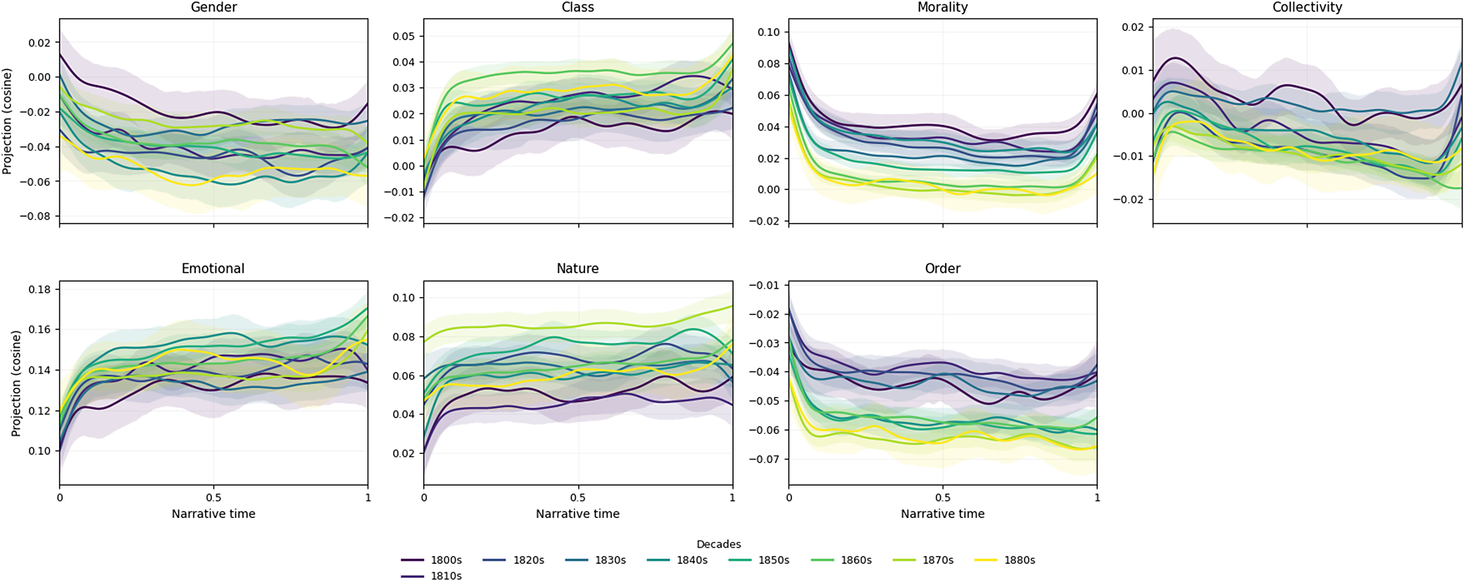
Figure 3 Long description
The multi-panel figure consists of seven line graphs arranged in two rows. The top row contains four panels: Gender, Class, Morality, and Collectivity. The bottom row contains three panels: Emotional, Nature, and Order.
Each graph plots ‘Narrative time’ from 0 to 1 on the X-axis against ‘Projection (cosine)' on the Y-axis. Ten colored lines represent decades from the 1800s (dark purple) to the 1890s (bright yellow), each with a shaded 95% C I (Confidence Interval) band.
* Gender: Shows a general downward trend in cosine values over narrative time, with earlier decades (darker lines) starting higher than later decades.
* Class: Features an initial sharp increase from 0 to 0.2 narrative time, followed by a plateau. Later decades (yellow/green) generally maintain higher projection values than earlier ones.
* Morality: Displays a U-shaped curve with high values at the start and end of the narrative. There is a clear vertical separation where earlier decades (purple) are significantly higher than later decades (yellow).
* Collectivity: Shows fluctuating, relatively flat trajectories centered around 0.00, with high overlap between decades.
* Emotional: All decades show a rapid rise in the first 20% of narrative time, stabilizing between 0.12 and 0.16.
* Nature: Shows a steady, slightly upward linear trend. Later decades (light green) occupy the highest projection space, while the 1800s (dark purple) occupy the lowest.
* Order: Displays a downward trend. Earlier decades (purple) maintain higher values (around -0.04) compared to later decades (yellow), which drop toward -0.07.
A legend at the bottom identifies the color gradient for the decades from 1800s to 1890s.
We also see a shift in sociodemographic variables. On the gender axis, we observe books adopting, on average, more female gender-coded language throughout the century. The class axis shows a shift, generally, from lower to higher classed language, with a trend toward increasing class trajectories (suggestive, possibly, of class aspirational novels), although there is some leveling off in this trend over time.
Genre trends
We next evaluate our analysis on genre exemplars, by selecting texts widely recognized as comedic or tragic and measuring mean sequence differences. We start with all Shakespearean tragedies and comedies (Figure 4), since these are known to adhere to a consistent and reasonably strict stylistic form. We then evaluate genre differences on widely recognized nineteenth century comedies and tragedies (Figure 5). We finally measure the similarity between all books and our genre exemplars in a single plot (Figure 6). We confirm that sequence measurements on our seven axes differentiate genre in broadly recognizable ways.
Shakespearean genre. Mean sequences (smoothed, bootstrapped 95% CIs) for all Shakespearean comedies versus tragedies. Comedies: “All’s Well That Ends Well,” “As You Like It,” “The Comedy of Errors,” “Love’s Labour’s Lost,” “Measure for Measure,” “The Merchant of Venice,” “The Merry Wives of Windsor,” “A Midsummer Night’s Dream,” “Much Ado about Nothing,” “Pericles, Prince of Tyre,” “The Taming of the Shrew,” “The Tempest,” “Twelfth Night; Or, What You Will,” “The Two Gentlemen of Verona,” “The Winter’s Tale,” “Cymbeline.” Tragedies: “Antony and Cleopatra,” “Coriolanus,” “Hamlet, Prince of Denmark,” “Julius Caesar,” “King Lear,” “Macbeth,” “Othello, the Moor of Venice,” “Romeo and Juliet,” “Timon of Athens,” “Titus Andronicus,” “Troilus and Cressida.”
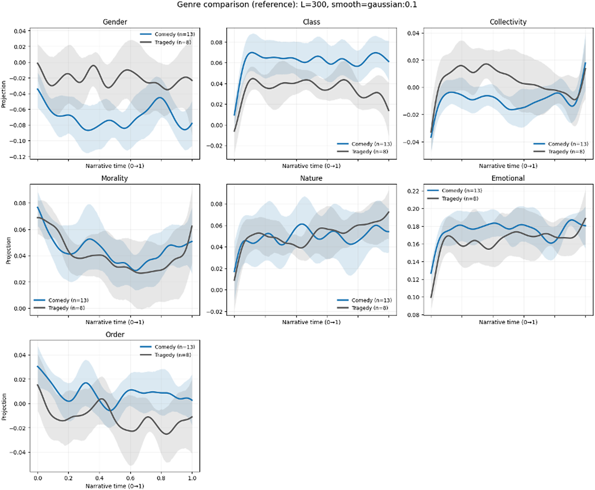
Figure 4 Long description
The figure consists of seven line graphs arranged in three rows. Each graph shares a common X-axis labeled Narrative time (0 to 1) and a Y-axis labeled Projection. Blue lines represent Comedies (n = 13) and black lines represent Tragedies (n = 8), both with shaded 95% C I ribbons.
* Top-Left (Gender): The tragedy line remains consistently higher than the comedy line, though both fluctuate between negative 0.02 and negative 0.10.
* Top-Middle (Class): Comedies show a significantly higher projection (around 0.06) compared to tragedies (around 0.04) throughout the narrative.
* Top-Right (Collectivity): Tragedies generally maintain a higher projection than comedies, with both converging toward a sharp increase at the end of the narrative time.
* Middle-Left (Morality): Both genres start high (0.07 to 0.08), dip toward the middle of the narrative, and rise again at the end, with comedies slightly higher in the second half.
* Middle-Middle (Nature): Both genres show an upward trend, starting near 0.02 and ending near 0.06, with significant overlap in their confidence intervals.
* Middle-Right (Emotional): Both genres show a rapid initial increase, plateauing between 0.16 and 0.18, with comedies generally maintaining a slightly higher mean.
* Bottom-Left (Order): Comedies maintain a higher projection (above 0.00) while tragedies drop into negative values (down to negative 0.02) for most of the narrative.
Nineteenth century genre. Mean sequences (smoothed, bootstrapped 95% CIs) for nineteenth century comedies and tragedies. Comedies: “Vanity Fair,” “Pickwick,” “Emma,” “Three Men in a Boat,” “The Old Curiosity Shop,” “The Pickwick Papers,” “Northanger Abbey,” “Pride and Prejudice,” “The Importance of Being Earnest,” “The Adventures of Tom Sawyer,” “Tom Jones,” “Alice’s Adventures in Wonderland,” “Sense and Sensibility.” Tragedies: “The Scarlet Letter,” “Tess of the D’urbervilles,” “Hedda Gabler,” “The Mayor of Casterbridge,” “The Sorrows of Young Werther,” “Crime and Punishment,” “Far From the Madding Crowd,” “Agnes Grey,” “Jude the Obscure,” “Anna Karenina,” “A Doll’s House,” “Madame Bovary,” “Ghosts,” “Moby Dick,” “The Idiot,” “Wuthering Heights.”
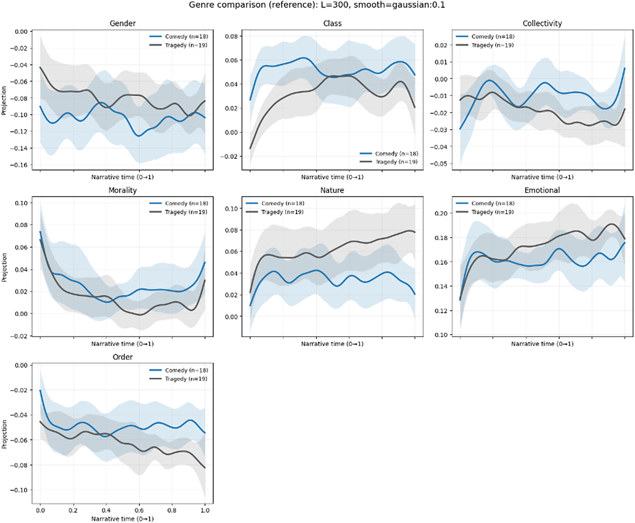
Figure 5 Long description
A multi-panel figure containing seven line graphs arranged in three rows. Each graph plots Projection on the y-axis against Narrative time from 0 to 1 on the x-axis. Two data series are shown in each: Comedy (blue line, n equals 18) and Tragedy (dark gray line, n equals 19), both with shaded 95% C I s.
* Gender: Tragedy starts higher at negative 0.04 and remains above Comedy, which fluctuates around negative 0.10.
* Class: Comedy maintains a higher projection than Tragedy throughout, with both peaking mid-narrative.
* Collectivity: Comedy fluctuates between negative 0.01 and 0.01, generally staying above Tragedy, which trends downward toward negative 0.03.
* Morality: Both start high at 0.07 and drop sharply. Comedy stabilizes around 0.02, while Tragedy stays lower near 0.00 before a late rise.
* Nature: Tragedy shows a steady upward trend from 0.02 to 0.08, consistently higher than Comedy, which fluctuates around 0.04.
* Emotional: Both series trend upward from 0.13. Tragedy rises more steeply, ending near 0.18, while Comedy ends lower near 0.17.
* Order: Both series trend downward. Comedy remains higher, ending near negative 0.05, while Tragedy drops more sharply to negative 0.08.
Composite semantic axis genre plot with labeled examples, using cosine similarity (per arc) to genre labels. Composite arcs are formed through concatenating semantic axis projection vectors and z-scoring. Comedies and tragedies are the same as in Figure 5, except with the addition of a small set of exemplars from Figure 4.
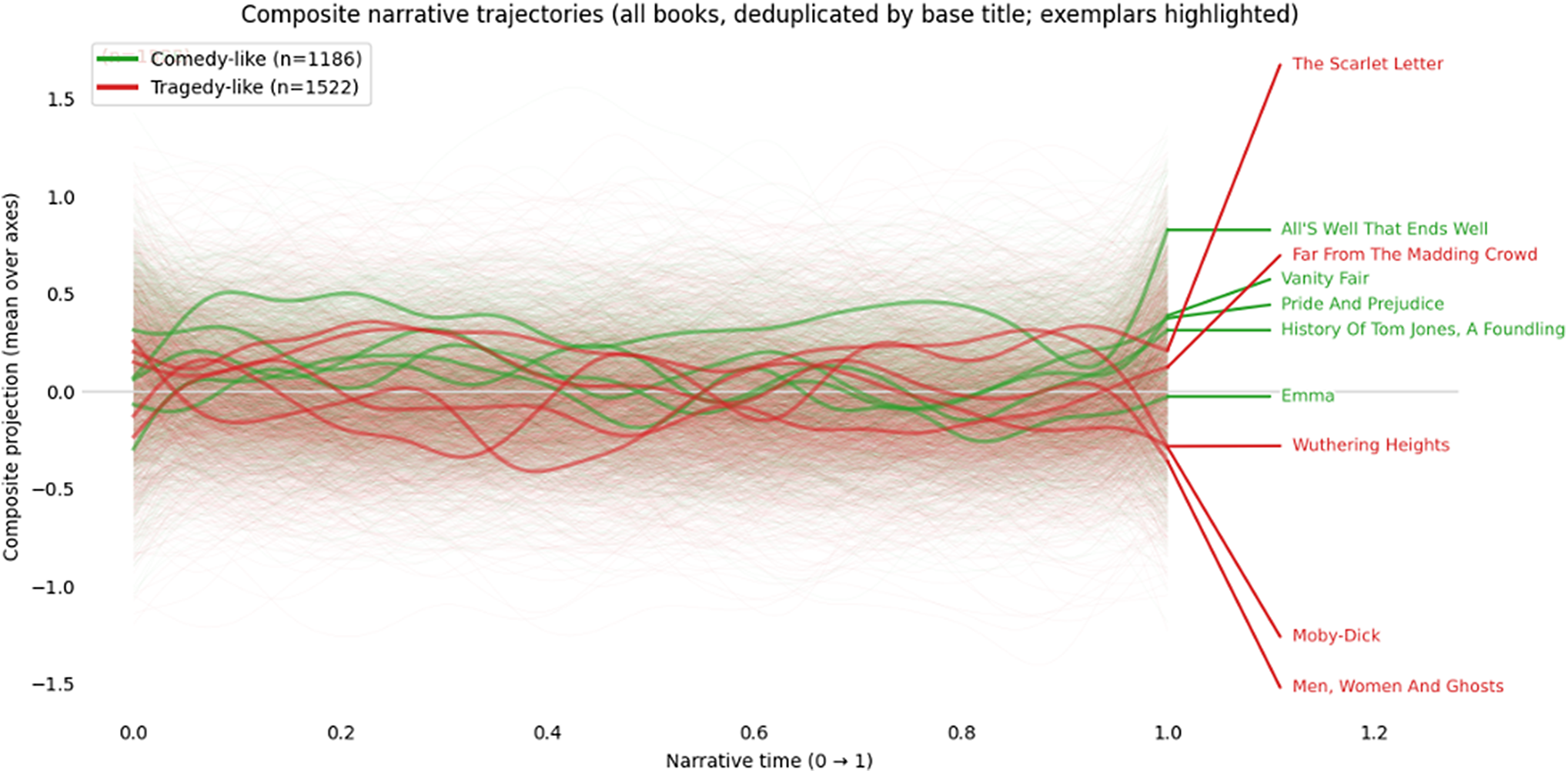
Figure 6 Long description
The X axis represents Narrative time from 0 to 1. The Y axis represents Composite projection mean over axes ranging from negative 1.5 to 1.5. A horizontal zero line serves as the baseline. The graph contains a dense cloud of faint lines with several bolded exemplar trajectories.
Legend at the top left:
* Green line: Comedy-like n equals 1186.
* Red line: Tragedy-like n equals 1522.
Exemplar trajectories fluctuate across the timeline and are labeled on the right side. From top to bottom, the labels and their corresponding line colors are:
* The Scarlet Letter (Red)
* All'S Well That Ends Well (Green)
* Far From The Madding Crowd (Red)
* Vanity Fair (Green)
* Pride And Prejudice (Green)
* History Of Tom Jones, A Foundling (Green)
* Emma (Green)
* Wuthering Heights (Red)
* Moby-Dick (Red)
* Men, Women And Ghosts (Red)
Green lines generally trend toward positive values at the end of the narrative time, while red lines show more varied terminal points, with several dipping into negative values.
Shakespearean genre categories, while complicated in many texts, follow a consistent typology over a single corpus so are a helpful narrative benchmark for our method. Comedies are often observed as breaking away from collective moral norms into individual freedom (typically to another geographic location, e.g., the pastoral “green world”) and then returning to collective norms again, whereas tragedies often involve a shift from collective moral integration toward exclusion and individual isolation alongside a shift from order to disorder. This is recognized broadly, including in, for example, Frye’s well-known genre taxonomy (Frye Reference Frye1957).
Our sequence models identify a similar pattern in the structure of narrative arcs segmented by genre. On the collectivity, order, and morality axes, comedies follow a roughly u-shaped arc, consistent with the idea that comedies represent a break from and return to collective moral order punctuated by a shift toward relative individualism and disorder. By contrast tragedies observe a gradual decline on the order, collectivity, and morality axes throughout. Comedies sit higher on the class and emotional/rational axis than do tragedies. The strongest distinction between genres is on the gender axis, where the u-shaped curve for comedies is potentially consistent with a tendency to cross-gender characters or invert the patriarchal order in the “green world” segment of most Shakespearean comedies. These trends do not of course “prove” genre-theoretic claims about formal narrative structure, but they are broadly consistent with such claims as aggregate patterns, suggesting the method is at least directionally compatible with existing structuralist narratological theory.
When we move to analyzing post-1700s genre, these sequence trends persist but compress – in other words, comedy and tragedy start to move toward similar formal structures. This is consistent with general understandings of genre and the rise of the novel, which see the novel form as collapsing what was once strict comedy and tragedy into increasingly hybrid narrative form (Bakhtin Reference Bakhtin2010; Lukács Reference Lukács1974). One of the larger changes compared to Shakespearean genre occurs on the emotional axis, where nineteenth century tragedy appears to shift further away from reason and toward emotion and the nature axis (i.e. away from artificial and social). Finally, the composite genre plot in Figure 6 suggests that extending genre exemplars to the whole corpus along our semantic axes seems to differentiate the forms roughly. We include this example as illustrative, but it is not meant as a formal classification.
Gender trends
We next segment trajectories by gender.Footnote 7 To do this, we label author by gender using the NLTK names list. We then scan for quotations in all texts to extract dialogue and label the speaker using a heuristic method. To detect speaker gender identity, we use a heuristic approach wherein we scan for quotations with length greater than two tokens, then check within a 20-token window outside the quotation for gendered names or for the pronouns “he” or “she.” We scan from the start of the quotation, for example, 10 tokens back and 10 tokens forward. This heuristic is expected to introduce some mismatches, such as when multiple names interact. It will fail to tag cases in long dialogue sections without name designations, which are common in fiction. Our results should thus be thought of as a conservative baseline that systematically overlooks dialogue turn-taking examples and complex coreference. However, we find our approach is generally robust as a conservative sampling heuristic; we manually evaluate a 200-label sample and find the accuracy is high at 0.94. We then plot mean trajectories, for our seven semantic axes, for female/male writers and female/male speakers (Figure 7). This allows us to measure variation in the representation of female versus male speakers.
Author–speaker gender projections.
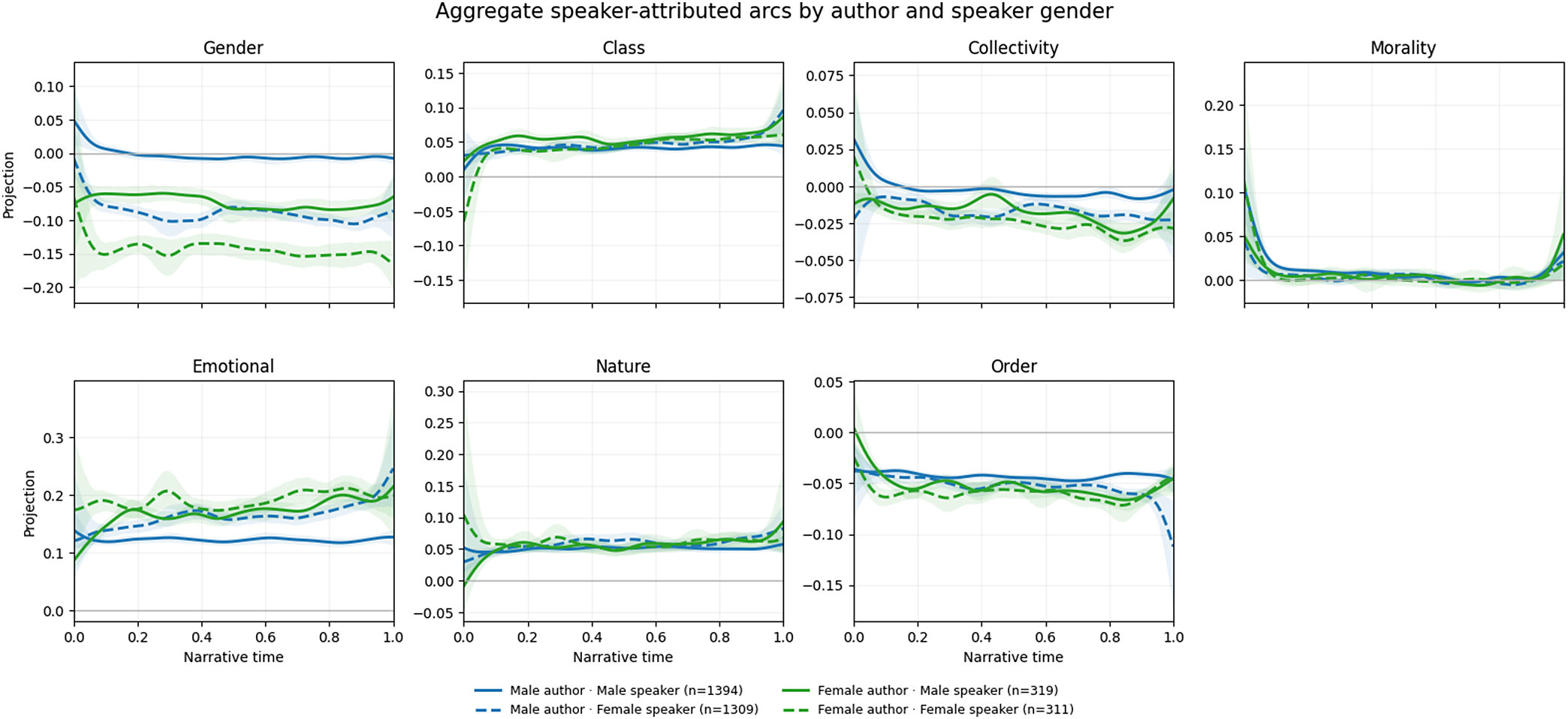
Figure 7 Long description
A multi-panel figure containing seven line graphs arranged in two rows. The X-axis for all graphs is Narrative time from 0.0 to 1.0. The Y-axis is Projection, with varying scales. Each graph contains four lines: solid blue (Male author - Male speaker), dashed blue (Male author - Female speaker), solid green (Female author - Male speaker), and dashed green (Female author - Female speaker). Shaded areas represent confidence intervals.
Top Row:
1. Gender: Male author - Male speaker starts high (0.05) and levels at 0.0. Other series remain negative, with Female author - Female speaker being the lowest at -0.15.
2. Class: All series show a slight upward trend from 0.0 to 0.10. Female author - Male speaker ends with the highest projection.
3. Collectivity: Most series hover between 0.0 and -0.025. Male author - Male speaker starts highest at 0.03 then drops.
4. Morality: All series start high (0.10 to 0.20), drop sharply to near 0.0 by 0.2 narrative time, and remain flat until a slight uptick at the end.
Bottom Row:
5. Emotional: All series trend upward from 0.1 to 0.2. Female author series show more variance than male author series.
6. Nature: Series are clustered around 0.05. Male author - Male speaker starts at 0.10 and drops, while Female author - Male speaker starts at 0.0 and rises.
7. Order: All series are negative, generally trending between -0.03 and -0.07. Male author - Female speaker shows a sharp drop at the end of narrative time.
Legend at the bottom indicates sample sizes: Male author - Male speaker (n=1394), Male author - Female speaker (n=1309), Female author - Male speaker (n=319), and Female author - Female speaker (n=311).
The aim of this analysis is to trace historical representational constraints on how gender is voiced and constructed, how standpoint influenced constructed representational positioning, and how gendered positions were articulated by women writers developing the early novel form’s construction. We contextualize trajectory results: women authors in this sample (at pooled mean) voice male and female characters closer to the female-coded axis than male authors, suggesting that while (as structuralist and narrative gender theory predicts) a gender-coded voicing repertoire existed, women writers may have shifted its representational center of expression across genders in this sample of the corpus. We further observe this when, for instance, women writers appear to construct male character dialogue that ranges further on the emotional versus rational axis than male writers do in this sample generally, suggesting a possible semantic re-centering with respect to how masculinity was constructed and engaged inter-textually (male characters start out around parity but follow arcs toward heightened affectivity, congruent with some recent arguments on nineteenth century reworking of masculine discourses). Potentially consistent with feminist narratological theory, female character dialogue also tends to be represented slightly (although not markedly) higher on individuality than collectivity, congruent with the influential claim in feminist narratology that female-coded characters were historically structurally positioned and voiced outside of a male-coded social collective (while often functioning to subvert or critique it). These findings are corpus-level and do not, on their own, establish claims from structuralist and feminist narratology, but they appear interpretively compatible with long-influential claims in feminist narratology. Individual text variance is quite high especially on constructs of interest above, indicating that writers were not strictly constrained by these trajectories at the individual book level, but that they also may represent possible field positions (mean absolute deviation gender = 0.101, class = 0.060, morality = 0.045, collectivity = 0.037, emotional = 0.116, nature = 0.072, and order = 0.053).
The aim of these analyses is to explore, as articulated in postclassical gender critiques of classical narratology, how gender standpoint might have informed patterned departures from formal narratological expectations shaped within a gendered literary field, particularly as women novelists became increasingly prominent over the nineteenth century. Feminist narratology has broadly emphasized how the male gaze (de Lauretis Reference de Lauretis1987) and patriarchal norms (Gilbert and Gubar Reference Gilbert and Gubar2020) constrained the kinds of narrative roles historically expected of female characters and the stylistic expectations of women writers, often placing female characters in marginal or subversive roles. Miller (Reference Miller1980) explicitly emphasized how genre forms promoted male-coded themes, such as coming of age. Lanser (Reference Lanser1992) highlighted how narrative perspectives, especially those speaking collectively, were historically male-coded. Warhol (Reference Warhol1989) argues by contrast that female-coded narrative speech was often articulated directly or personally.
We can interpret the trajectory plots as reinforcing some of these arguments. For instance, women writers, in positioning female characters as progressively breaking from normative collectivity – seen here on the collectivity axes – might cohere with Gilbert and Gubar’s (Reference Gilbert and Gubar2020) argument that female characters were frequently positioned in subversive roles formally opposed to a masculine-coded notion of the universal collective (Lanser Reference Lanser1992). This is only one possibility, however, suggested by the aggregate curves, not an evinced finding, and significant close reading and supporting analysis would be required to further interrogate whether this particular trend is motivated by this postclassical narratological argument or not.
Relational trajectory space analysis
So far, we have interpreted aggregate trends; however, our model is also conducive to a relational interpretation of narrative form if we conceptualize it in terms inspired by (though not technically identical with) functional data analysis. In the above visualization (Figure 8), we run PCA on trajectory chunks for the four axis projections (morality, collectivity, gender, and class) after z-scoring and find that PCA separates a space of functional curve forms – PC2 (the y-axis) distinguishes inverted u-shape and u-shaped curvature (top to bottom) and PC1 distinguishes ascending versus descending curvature (left to right).Footnote 8 Each cutout plots 150 books with 0.25 Gaussian smoothing, although these shapes are retained in unsmoothed curves, presented in the Supplementary Material. PCA with z-scoring yields the space of curve shapes above separating raw curve shapes while removing differences in amplitude and starting absolute position; PCA on sequences without z-scoring incorporates wave amplitude and absolute starting position. We can then analyze separation in the z-scored shape space or in its non-z-scored variant for various variables.
Recovering narrative curve types using PCA on sequence trajectory projections of four axes (gender, collectivity, morality, and order). We construct vectors composed of four projection values per chunk, reduce with PCA, and find that PC1 captures ascending to descending curve shapes, and PC2 captures u-shaped to inverted u-shaped curve shapes, consistent with functional PCA analysis. We can then analyze how narratives distribute within this space of curve types. Recovered curve shapes visually deteriorate with null model tests, reported in the Supplementary Material, along with a variant with all seven axes.
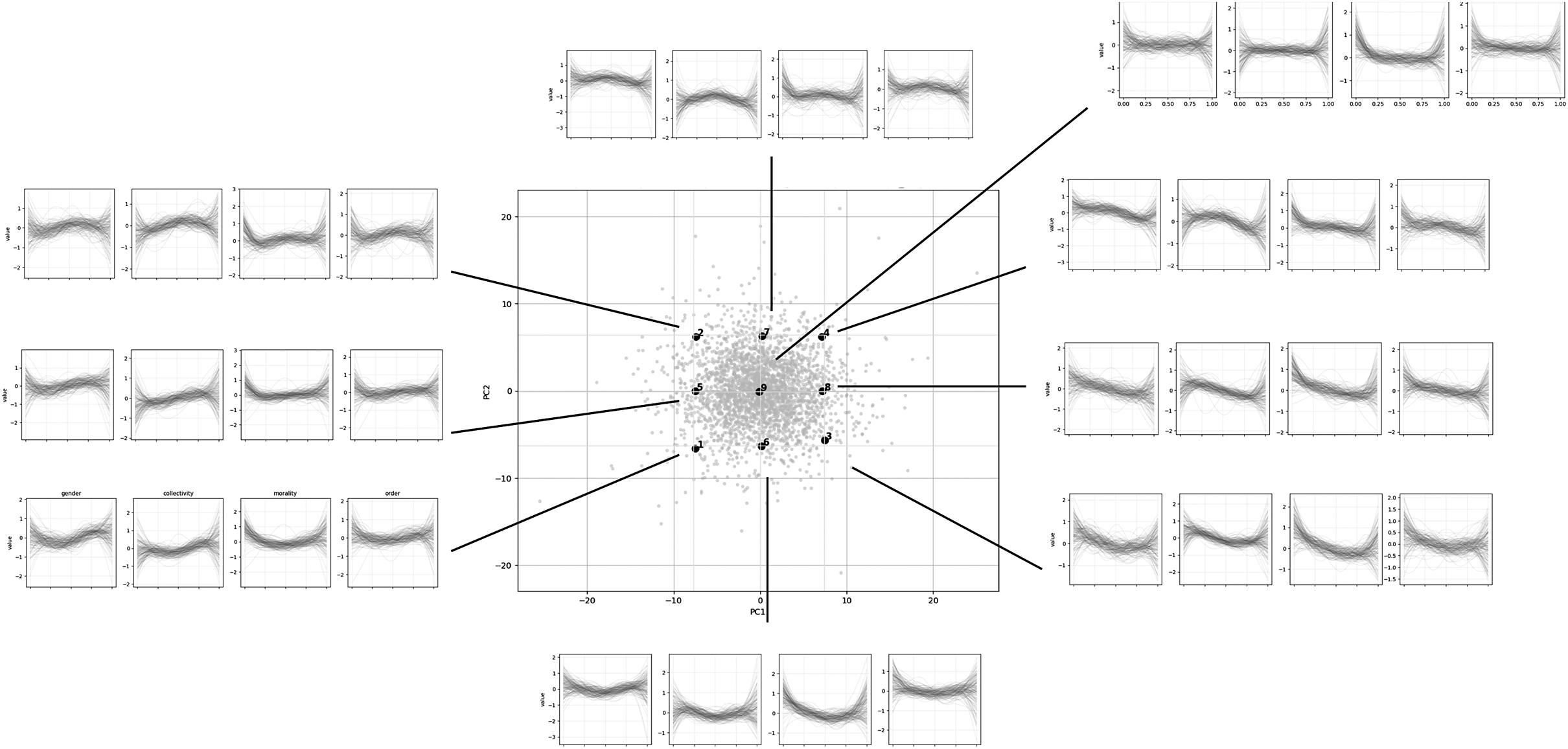
Figure 8 Long description
A central scatter plot maps P C 1 on the x-axis from negative 20 to 20 and P C 2 on the y-axis from negative 20 to 20. Nine numbered points are distributed in a grid within the central cluster of gray data points. Eight lines radiate from this center to peripheral clusters of line graphs. Each peripheral cluster contains four small line graphs labeled gender, collectivity, morality, and order.
Moving clockwise from the top-left:
* Top-left cluster: Curves show an ascending trend.
* Top-center cluster: Curves show an inverted u-shape, peaking in the middle.
* Top-right cluster: Curves show a descending trend.
* Middle-right cluster: Curves show a more pronounced descending trend with a slight u-shape at the end.
* Bottom-right cluster: Curves show a deep u-shape, dipping in the middle.
* Bottom-center cluster: Curves show a shallow u-shape.
* Bottom-left cluster: Curves show an ascending trend with a slight dip at the start.
* Middle-left cluster: Curves show a flat or slightly oscillating horizontal trend.
The central point 9 represents the average or neutral state where curves are relatively flat across all four axes.
When we test this on Shakespearean genre using a reduced axis set expected to distinguish genre (collectivity, morality, order, and nature), we find using linear discriminant analysis that the z-scored PCA-reduced sequences accurately separate texts by genre (Figure 9). Based on the PCA results, comedies tend to follow descending and u-shaped arcs while tragedies tend to follow ascending, inverted u-shape, and stationary arcs on the four semantic axes. These are composite results of the four axes, but they reflect u-shaped collectivity curves for comedy and possibly inverted u-shape collectivity curves for tragedy, ascending nature curves for tragedy, possible inverted u-shape order curves for tragedy, and u-shaped morality curves for comedy. This is consistent again with the earlier treatment of, for example, Frye’s genre, wherein comedies move in u-shape away from and toward collective and moral integration, and where tragedy involves shifts away from earlier moral and collective integration.
Distribution of genre (Shakespearean) in PCA curve space. The model, without supervision, appears to separate comedy and tragedy into ascending/u-shaped versus descending/inverted u-shaped or stationary arcs. It also locates “problem plays,” romances, or genre ambiguous texts at the boundary of the two. Axis effect sizes (Cohen’s d) are collectivity = 0.135, morality =
$-$
 0.113, nature =
$-$
0.113, nature =
$-$
 0.244, and order =
$-$
0.244, and order =
$-$
 0.319.
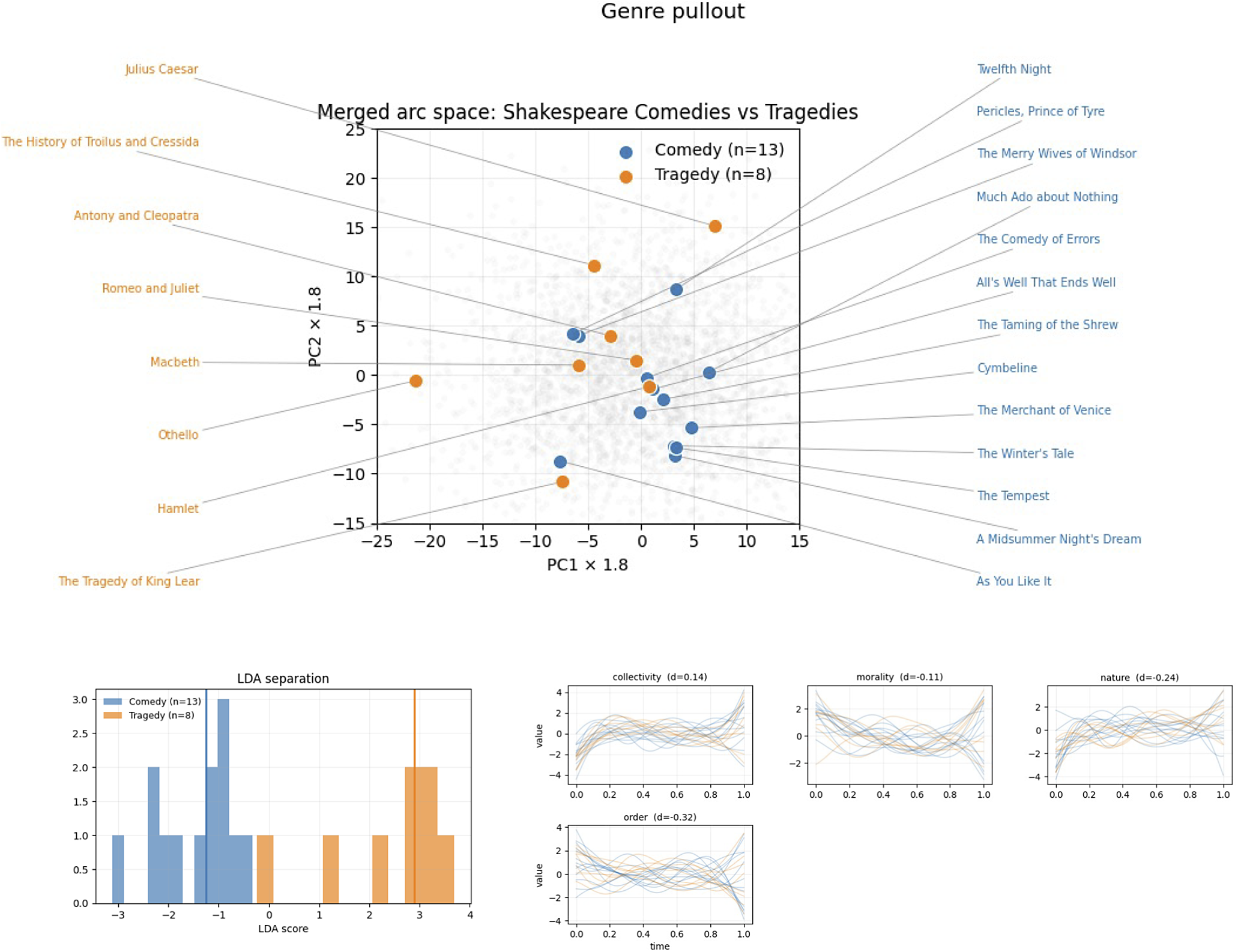
Figure 9 Long description
The top panel is a scatter plot titled Merged arc space: Shakespeare Comedies vs Tragedies. The x-axis is P C 1 times 1.8 ranging from minus 25 to 15, and the y-axis is P C 2 times 1.8 ranging from minus 15 to 25. Blue dots represent Comedy (n=13) and orange dots represent Tragedy (n=8). Lines connect specific dots to play titles on the margins. On the left, tragedies like Julius Caesar, Macbeth, and Hamlet are clustered. On the right, comedies like Twelfth Night, Much Ado about Nothing, and As You Like It are positioned.
The bottom-left panel is a histogram titled L D A separation. The x-axis is L D A score from minus 3 to 4. Blue bars for Comedy are concentrated between minus 3 and 0, while orange bars for Tragedy are concentrated between 1 and 4, showing clear categorical separation.
The bottom-right section contains four small line graphs showing value over time from 0.0 to 1.0.
* Collectivity (d=0.14) shows blue and orange lines fluctuating around zero with a slight upward trend at the end.
* Morality (d=minus 0.11) shows U-shaped and inverted U-shaped curves.
* Nature (d=minus 0.24) shows a dense cluster of arcs peaking in the middle.
* Order (d=minus 0.32) shows diverging arcs that spread wider as time approaches 1.0.
We next test whether our PCA curve space distinguishes other variables such as time period. For time period, we test the model’s ability to distinguish the early and late 1800s, and we report in Figure 10 both non-z-scored (top) and z-scored results (bottom). We use all seven semantic axes to construct the PCA space. Again, z-scoring isolated curve shapes only, whereas non-z-scored results also separate data by absolute semantic projection scores (affecting starting separation and curve magnitudes). For time period trends, by contrast to genre, we find separation only for the non-z-scored plot. This suggests weak evidence in our model for changing plot trajectory shapes through time, but modest evidence for semantic shifts (on both absolute semantic drift and curve magnitude).
Plot trajectories separated by time yield similar distributions without z-scoring (top) and with z-scoring (bottom). Effect sizes (Cohen’s d) for PCA without z-scoring: gender = 0.101, class =
$-$
 0.229, collectivity = 0.287, morality = 0.745, emotional =
$-$
0.229, collectivity = 0.287, morality = 0.745, emotional =
$-$
 0.099, nature =
$-$
0.099, nature =
$-$
 0.272, order = 0.560; effect sizes for PCA with z-scoring: gender = 0.060, class = 0.068, collectivity =
$-$
0.272, order = 0.560; effect sizes for PCA with z-scoring: gender = 0.060, class = 0.068, collectivity =
$-$
 0.033, morality = 0.066, emotional = 0.031, nature =
$-$
0.033, morality = 0.066, emotional = 0.031, nature =
$-$
 0.002, and order = 0.098.
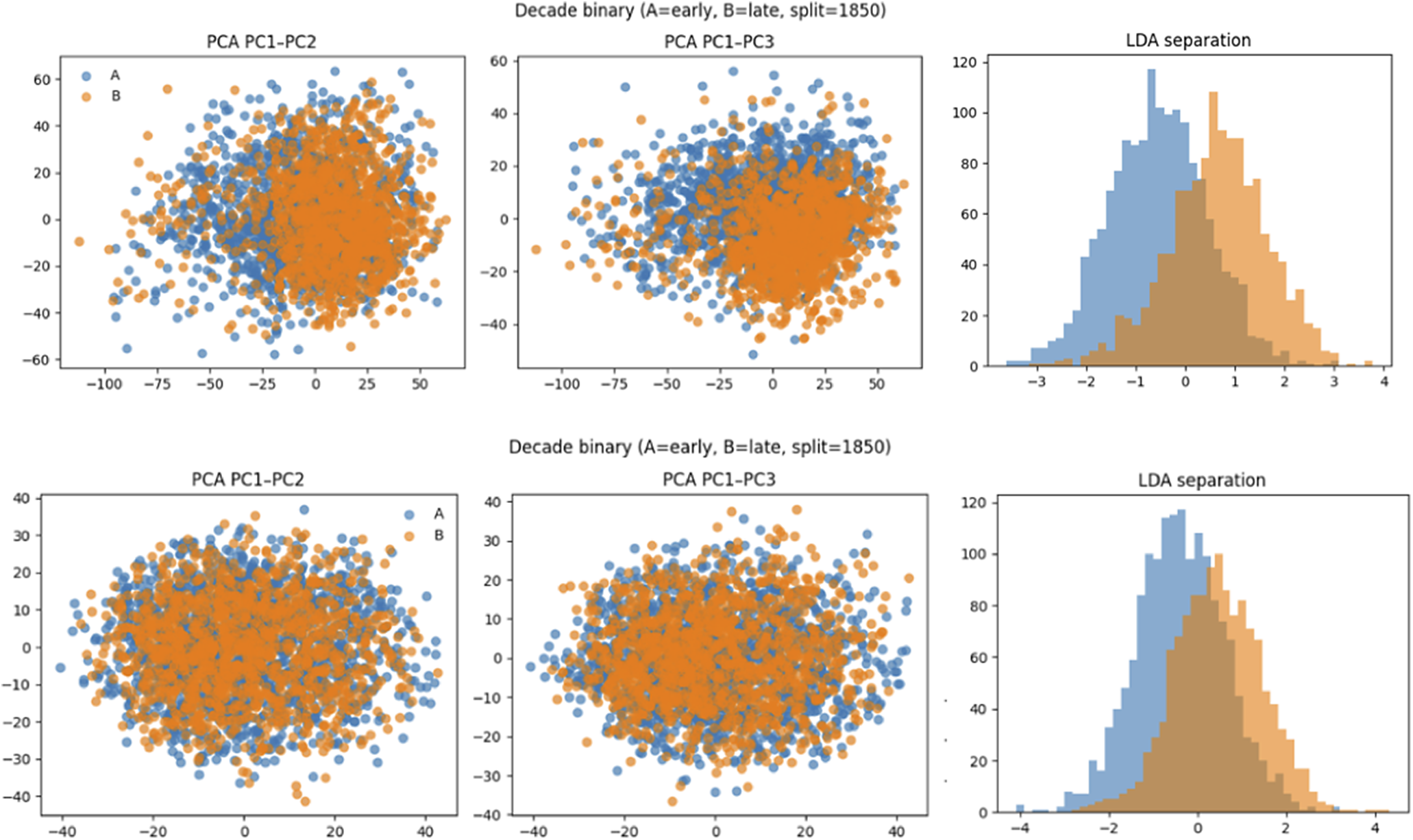
Figure 10 Long description
The figure is organized into two rows, each containing three panels.
Top Row: Decade binary (A equals early, B equals late, split equals 1850) without z-scoring.
* Left Panel: P C A P C 1-P C 2 scatter plot. Blue dots (A) and orange dots (B) are heavily overlapped in a large cluster centered near the origin, with a slight horizontal spread from negative 100 to 50 on the x-axis.
* Middle Panel: P C A P C 1-P C 3 scatter plot. Similar to the first panel, showing a dense, overlapping cluster of blue and orange points.
* Right Panel: L D A separation histogram. Two distinct but overlapping distributions. The blue distribution (A) peaks around negative 0.5, while the orange distribution (B) peaks around 1.0.
Bottom Row: Decade binary (A equals early, B equals late, split equals 1850) with z-scoring.
* Left Panel: P C A P C 1-P C 2 scatter plot. The data points are more tightly clustered and centered, with the x-axis range reduced to negative 40 to 40. Blue and orange points are almost entirely mixed.
* Middle Panel: P C A P C 1-P C 3 scatter plot. Shows a circular, highly mixed distribution of blue and orange points centered at 0, 0.
* Right Panel: L D A separation histogram. The blue and orange distributions show significantly more overlap than the top row, with both peaks shifting closer to 0. The blue peak is near negative 0.2 and the orange peak is near 0.8.
Discussion
We discuss what our results suggest as a prototype framework for embedding sequence analysis as well as implications of this technique more broadly for computational narratology. We also briefly synthesize our substantive results, interpreting their implications for narrative theory.
While word embeddings are routinely used in natural language processing, with contextual embeddings becoming increasingly popular since their introduction in 2017, embeddings have been less frequently used in time-series and sequence analysis. Our work most directly extends diachronic word embedding modeling, which traces how individual words change over time series, from corpus-level analysis to the analysis of individual text sequences. This article’s approach demonstrates that chunking embedded text and then pooling chunks to form sequence trajectories appears to generate interpretable, meaningful narrative sequence representations and that analyzing these representations in aggregate tracks known historical trends in narrative structural form.
Sequential time-series applications of language embeddings represent a midrange technique positioned between aggregate corpus statistics, which reduce books to a single data point, and classification and generative models, which are comparably more opaque. The fact that sequences, moreover, appear to encode coherent trends at the scale of
$\sim $
 3,000 books implies that representational learning may capture organization at scales rarely analyzed by common natural language benchmarks.
Our analysis remains preliminary and requires further experimentation, although the results presented here are promising and imply reasonable methodological robustness. Our use of contextual sampling from Project Gutenberg for axis construction is intended to extend axis construction to contextual embedding models applied to historical texts. While this is theoretically validated as an extension of prior work such as Lucy, Tadimeti, and Bamman (Reference Lucy, Tadimeti and Bamman2022), changing corpora or anchoring methods could change results. One limitation of this approach is that sentence transformers are trained on contemporary corpora, so while our semantic axes use historical examples, embedding representations may still project contemporary linguistic associations onto the historical corpus (a possibility we cannot rule out here). There are comparably few historical embedding models, and we think that the use of historically grounded semantic axes with sentence transformers partly obviates this limitation. However, this mismatch remains one of the stronger limitations today on applying contemporary natural language processing models to historical texts. A more comprehensive future validation could further consider stabilization on larger and multiple corpora and models. It could also consider fine-tuning embeddings, though fine-tuning can also erase or confound semantic associations.
As a contribution to narrative theory, our findings primarily complement and draw on well-known ideas from postclassical narratological theory. We provisionally capture widely theorized trends in the rise of the novel, such as shifts toward individualism and realism, as well as trends in the emergence and development of genre as it realizes itself in novel form. We also capture some evidence for trends developed by feminist narratology when segmenting texts by gender.
We note with caution some of the unique inferential limitations and caveats of our modeling assumptions. As noted earlier, chunking and embedding texts operate at a somewhat coarse level of granularity, although sentence transformers are designed to represent sequences uniquely. When we project sequences onto semantic axes, we nonetheless collapse local semantic variance into an average representation. Resampling and smoothing further collapse local semantic fluctuations into broader patterns. This is intended to isolate semantic tendencies that persist from local noise, though it risks collapsing some local variance (which can often be quite narratively rich), or dialectical constructs that signify by oscillating between semantic values.
The analysis of semantic axes is arguably one of the most widely used methods in NLP in the social sciences (with meaningful use in cultural analytics), and linear axes can frequently recover interpretable directions from natural language representations. They are not the only available technique for model interpretability or classification today, however, and they possess known limitations such as fragility to seed word choice (Antoniak and Mimno Reference Antoniak and Mimno2021). We engage them because they are interpretable, well tested, straightforward to validate, and computationally lightweight to integrate with our broader framework. Our validation results indicate that the selected axis seeds recovered meaningful, corpus-specific semantic directions from the sentence transformer model’s representational space.
One of the largest analytic concerns, however, with this kind of approach is that it might synthesize trends while blurring local semantic distinctions. We believe that our statistical robustness tests – especially time-shuffled null permutations and smoothing and resampling sensitivity analyses – generally point away from this possibility, though the risk remains inherent to this kind of analysis. Statistical variance observed in aggregate should be read as a floor rather than a ceiling on possible semantic trends and associations embedded in the corpus and further contextualized using close reading when applied in practice in order to mitigate these limitations.
Our corpus exhibits some noise – both due to Gutenberg metadata mismatches that allow nonfiction works to fall through and due to the inclusion of volumes, collected works, and anthologies such as poetry collections. It also includes introductions and non-fictional sections of variable length. Rather than manually correct for these in this article, we retain them and rely on a uniform book-length inclusion criterion – this generally yields a conservative estimate of fictional trends in our narrative trajectory curves. These issues likely introduce balanced noise rather than systematic bias, and our time shuffle null results strongly suggest that they do not fundamentally degrade the overall representations.
Where our technique may contain potential for its most novel contribution is in its capacity to analyze directly the constituent elements of narrative form – plot temporality – at large, aggregate scales rather than through generalization from micro-scale close reading. Structuralist theory and historical analysis, in conjunction with close reading, triangulates well between macro-historical narrative trends and their micro-formal articulation. However, the aggregate analysis of the constituent elements of narrative form – the conditional, patterned representation of content in time, order, or sequence rendered in the voices of specific characters – specifically captures the spirit of empirical aggregate analysis for which classical and postclassical narratological theory has repeatedly called, but for which statistical tools have been historically incomplete.
While our technique cannot mirror the hermeneutic density of close reading (nor does it aspire to), it can provide a potentially new way to interpret in the space between individual text and corpus-level pattern. In practice, for instance, we observed when reading individual text samples that our approach highlighted historically specific trends for several under-read or non-canonical sources, allowing corpus-scale analyses that may offer the potential to situate and elevate rather than reduce away constituent, marginal, or oppositional representations.
At the same time, we recognize caution is warranted in inferring strong conceptual generalization from our model’s outputs. Many of the constructs we engage – morality, individualism, reason, order, and disorder – are analytically complex and historically situational, if not notoriously evasive. Our model is on the other hand intentionally constructed as simple and parsimonious. This juxtaposition is partly deliberate – our aim is to inscribe as few assumptions as possible into our modeling strategy to test the degree to which conceptual generalities appear in aggregate as well as how they vary in particular expression. We intentionally include some fairly abstract concepts to test the potential range of this type of approach. This framework does not and cannot resolve them in their full, polyvalent expression – it sheds a certain kind of aggregate and general light on macro-level patterns that are often hard to capture through direct reading. Interpreting their meaning, however, is intentionally left as an exercise to the reader.
Conclusion
In conclusion, this article demonstrates a straightforward method for analyzing narrative sequences by embedding books as sequences of chunked text, projecting chunks onto semantic axes, and aggregating book-level sequences into corpus-wide sequences. We find that this approach is highly robust to initial statistical tests, such as within-book time shuffle nulls, and to chunking, resampling, and smoothing parameter variation. While there is more work to be done to validate our approach, we suggest that it shows promise for the analysis of sequential text data in general and narrative structure in particular. More broadly, the approach suggests a path toward modeling how meaning develops over time within texts rather than only how it is distributed across them.
Future work might consider alternatives to prespecified semantic axes, such as methods for inducing corpus-specific semantic dimensions, or adapting the method to alternative kinds of narratives (such as narratives embedded in speeches, scientific discourse, or online communication). One extension, for example, could apply it to video transcripts, to complement similar time-series multimodal models.
Supplementary material
The supplementary material for this article can be found at https://doi.org/10.1017/chr.2026.10035.
Data availability statement
All data for this project were drawn from the english_gutenberg dataset available on the HuggingFace data repository using the sampling strategy described in the article. Texts are in the public domain and free to use for research under Project Gutenberg’s license. To avoid duplicating the dataset, we do not include it here. For the out-of-domain ground truth tests, we include the sentence pairs in the Supplementary Material.
Acknowledgements
I am very grateful to the anonymous peer reviewers, whose suggestions helped considerably to strengthen this essay. Some code for the analysis was initially generated with the assistance of a language model and independently modified and verified by the author. The author takes full responsibility for the results and analysis.
Author contributions
Conceptualization: W.R.; Data curation: W.R.; Investigation: W.R.; Methodology: W.R.; Software: W.R.; Writing: W.R.
Funding statement
The author declares that no specific funding has been received for this article.
Competing interests
The author declares none.
Ethical standards
The research meets all ethical guidelines, including adherence to the legal requirements of the study country.

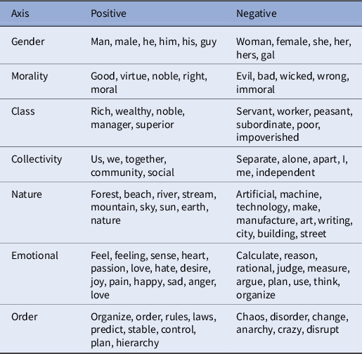
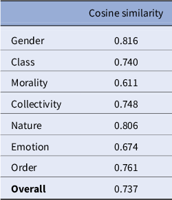
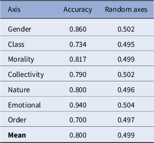
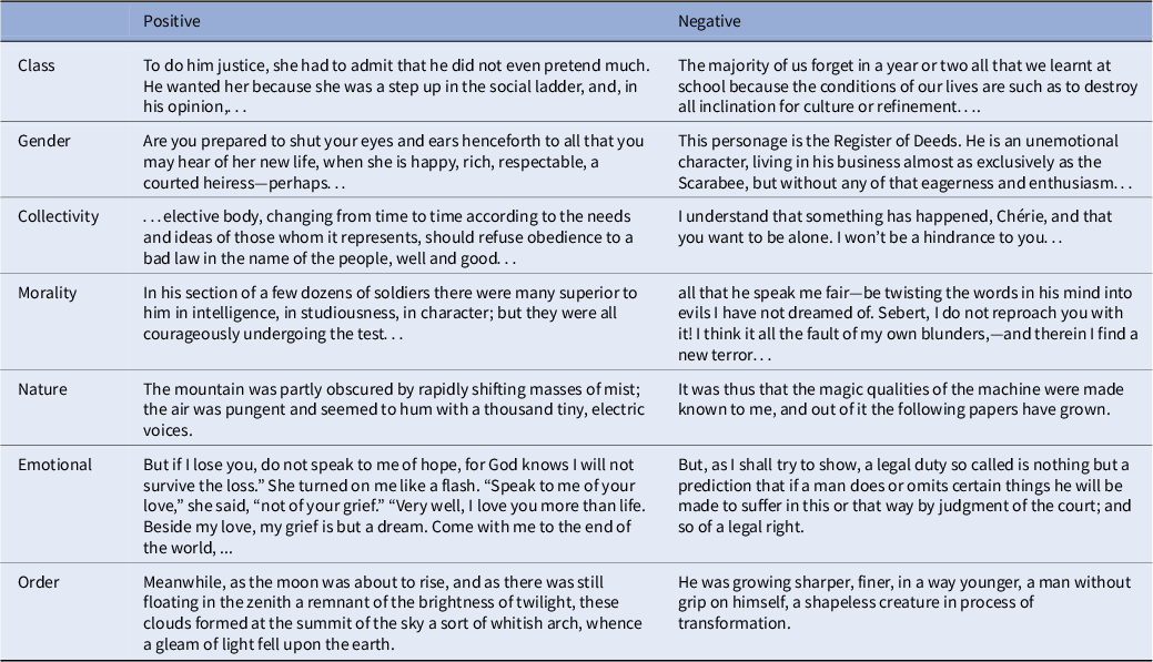
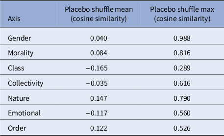
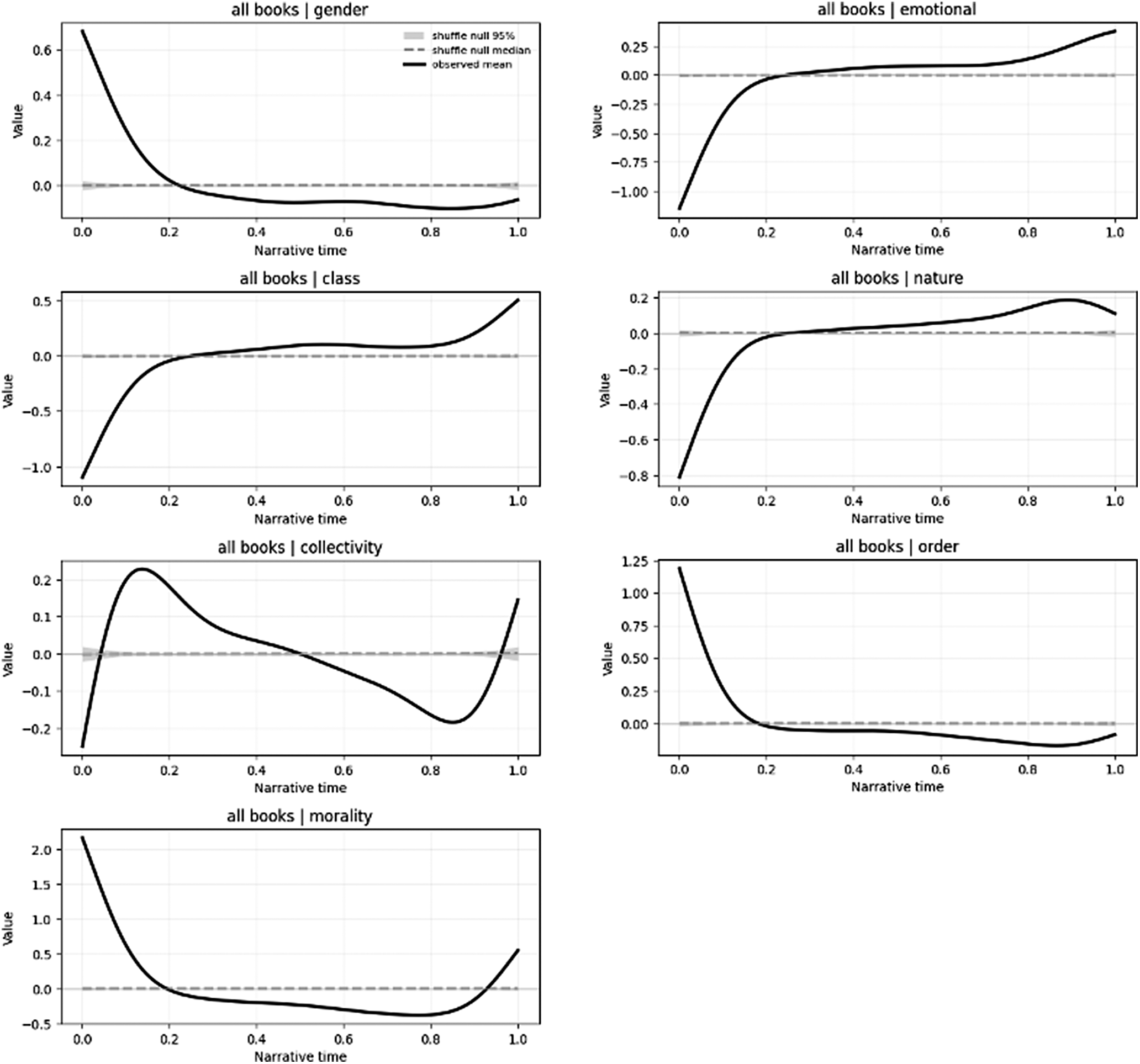

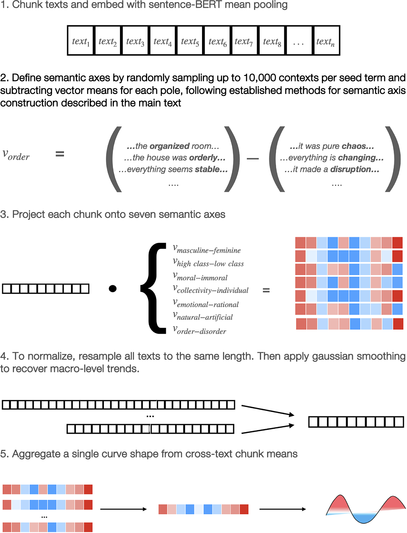
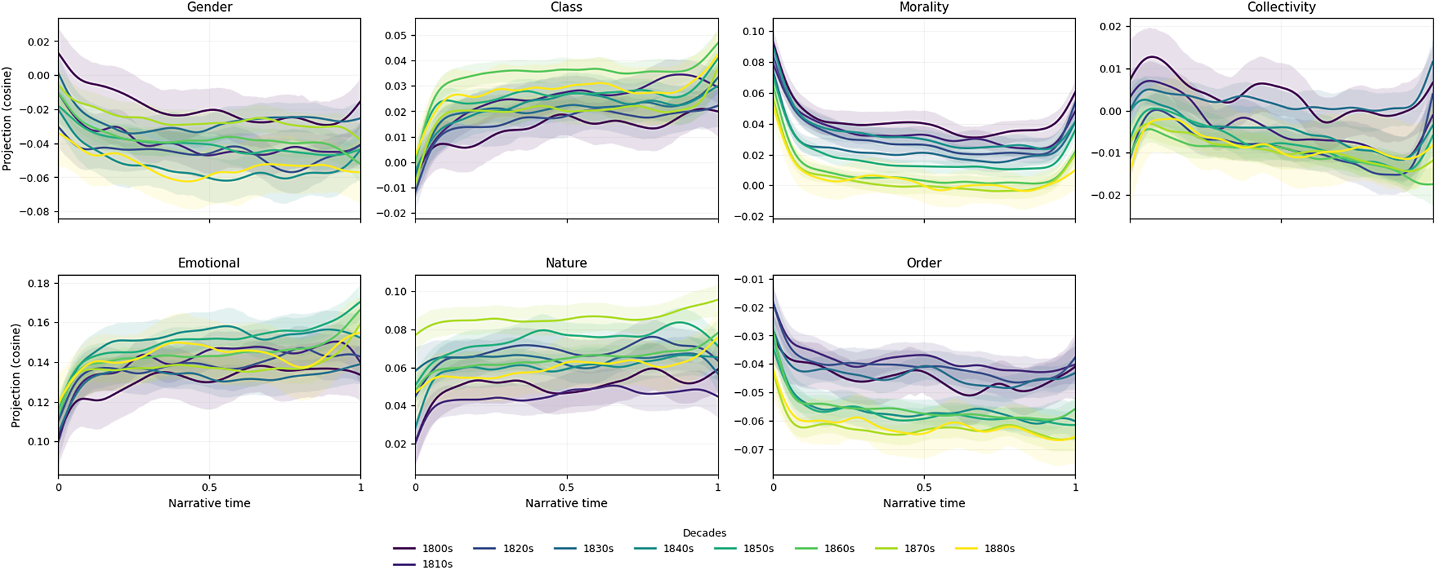
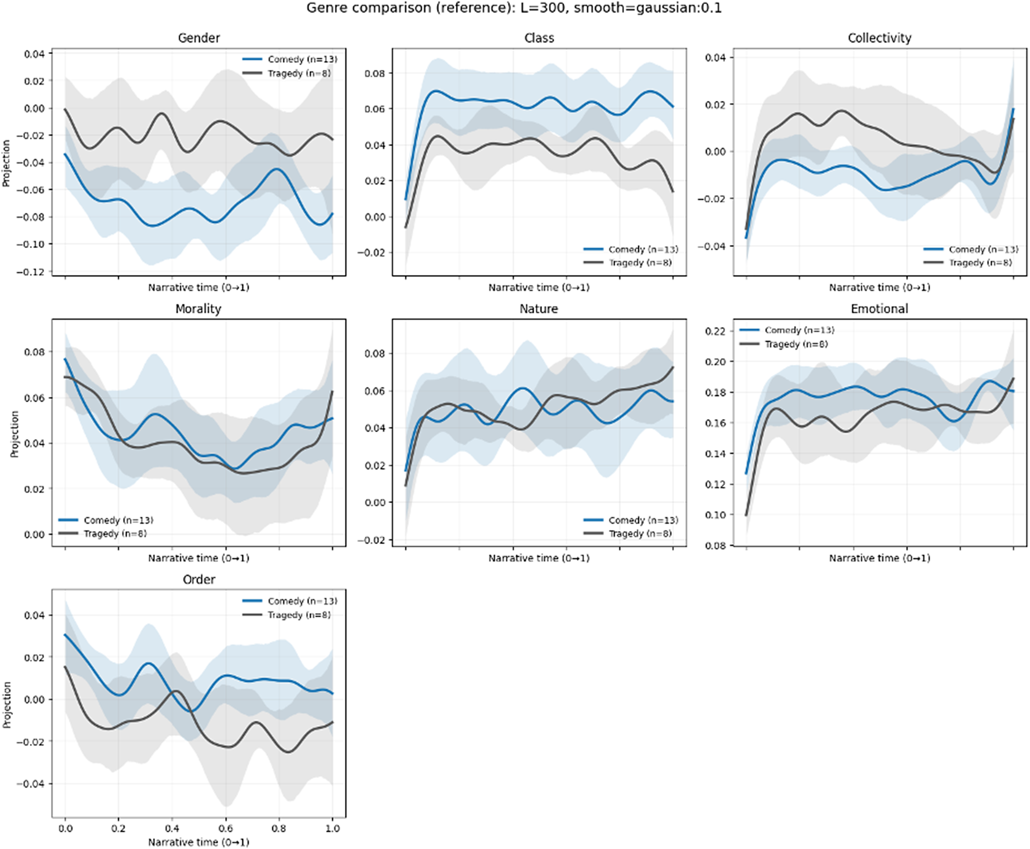
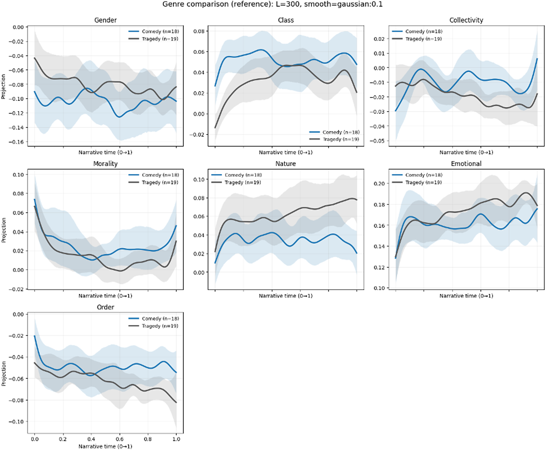
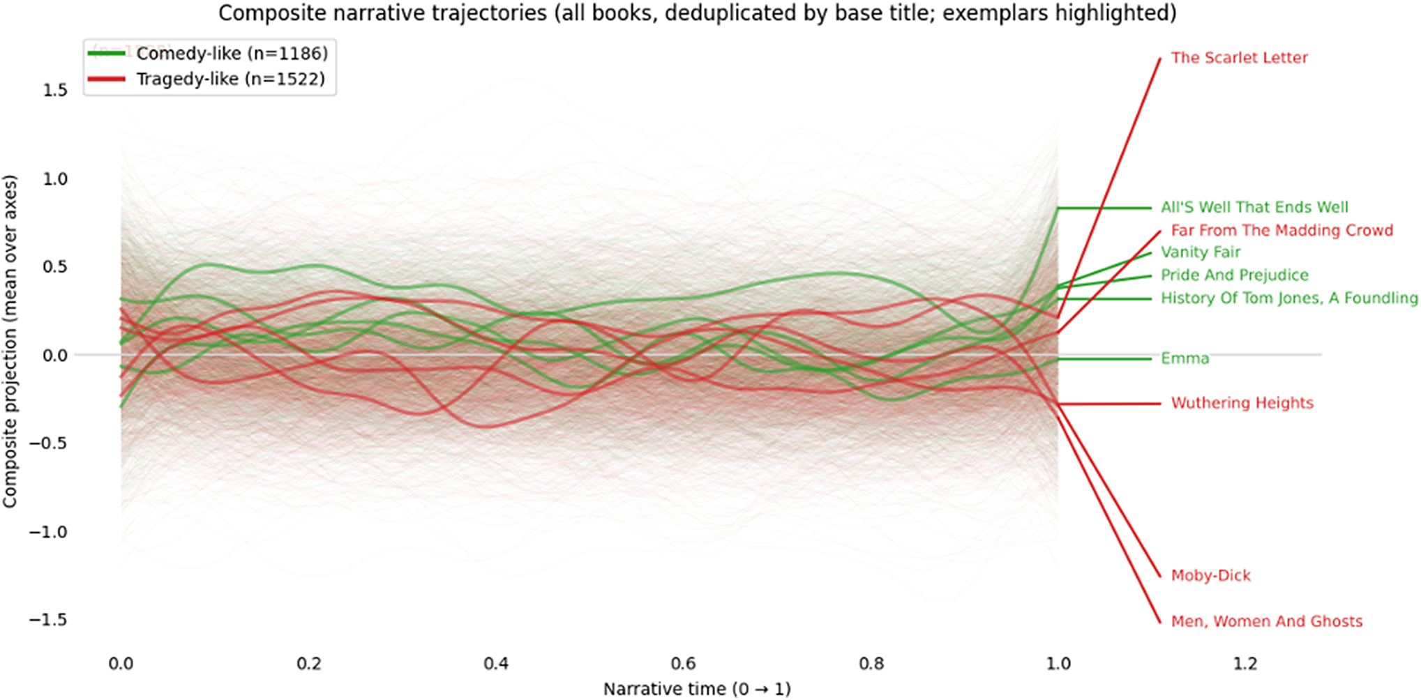
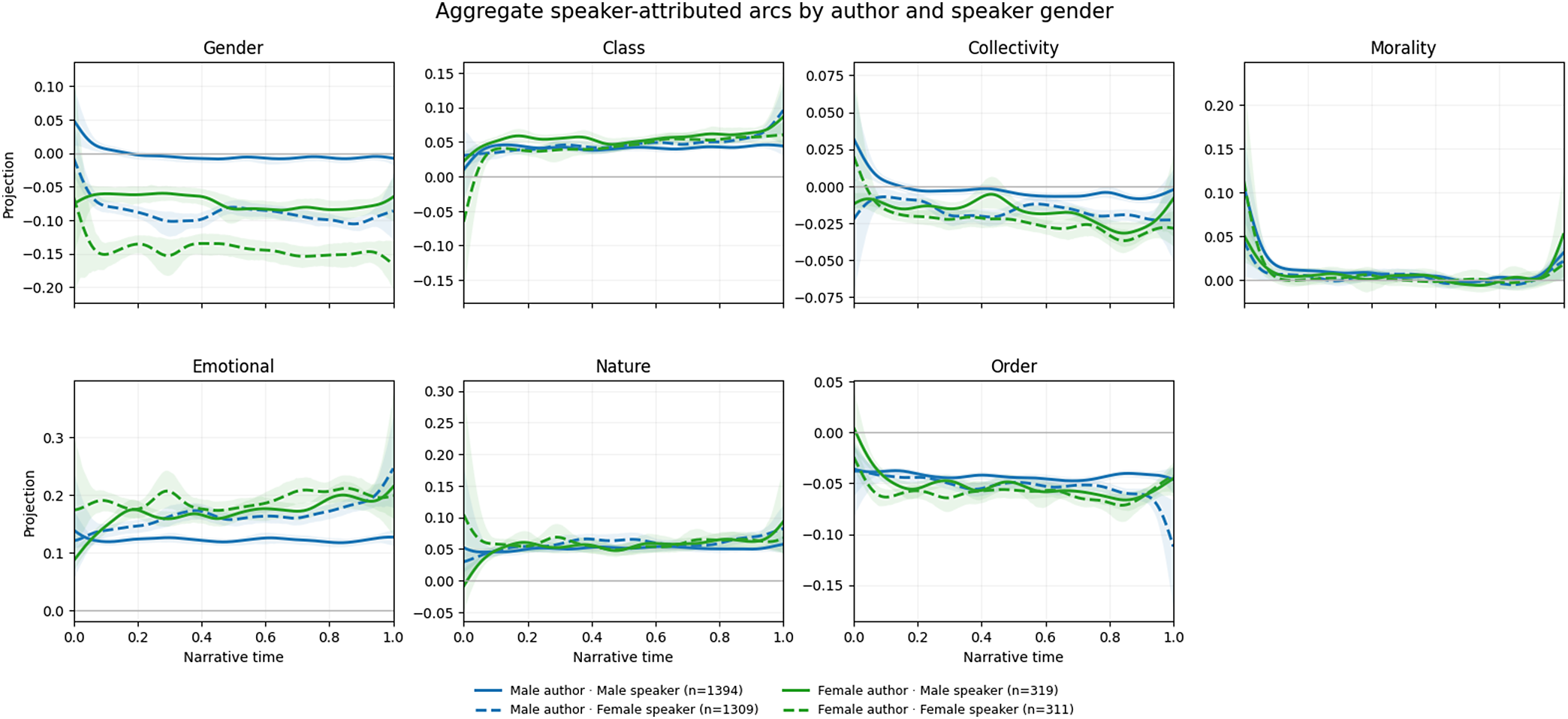
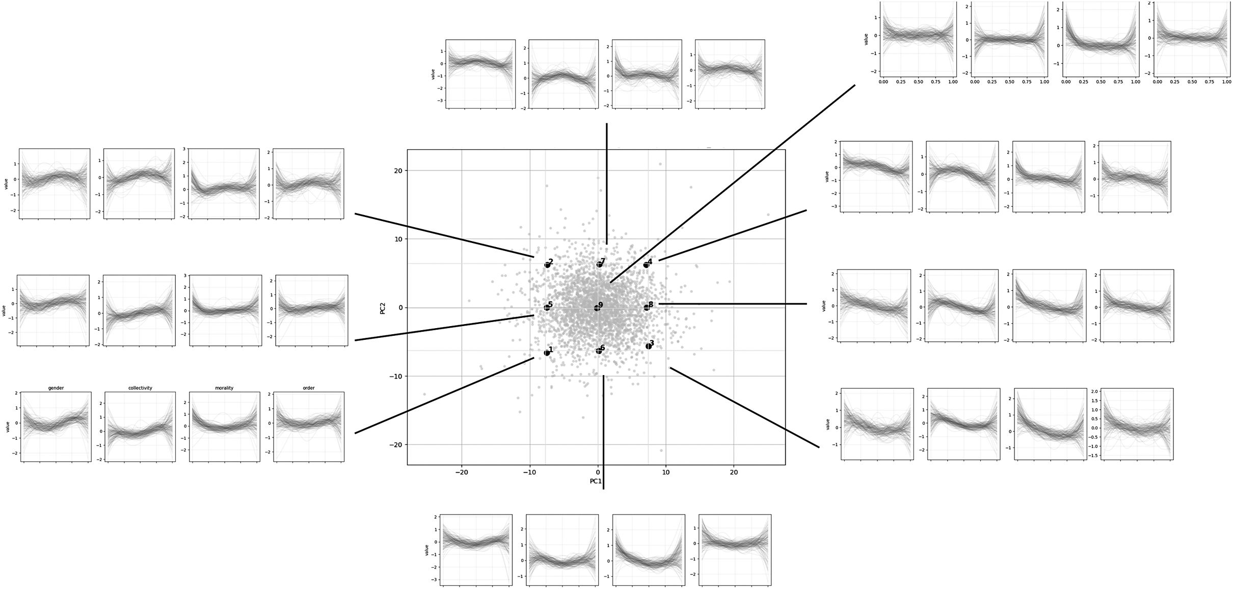
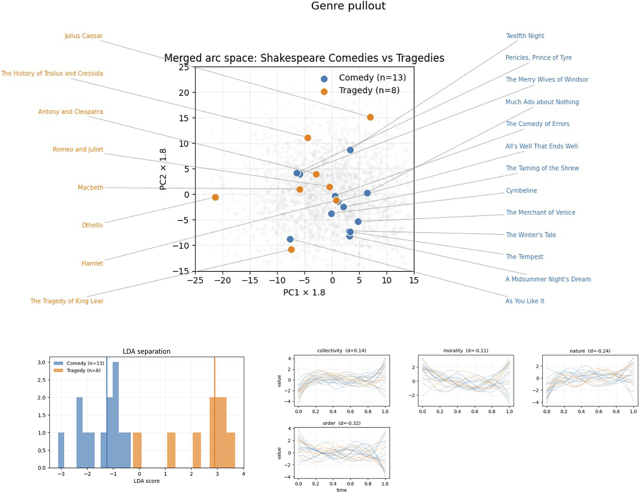


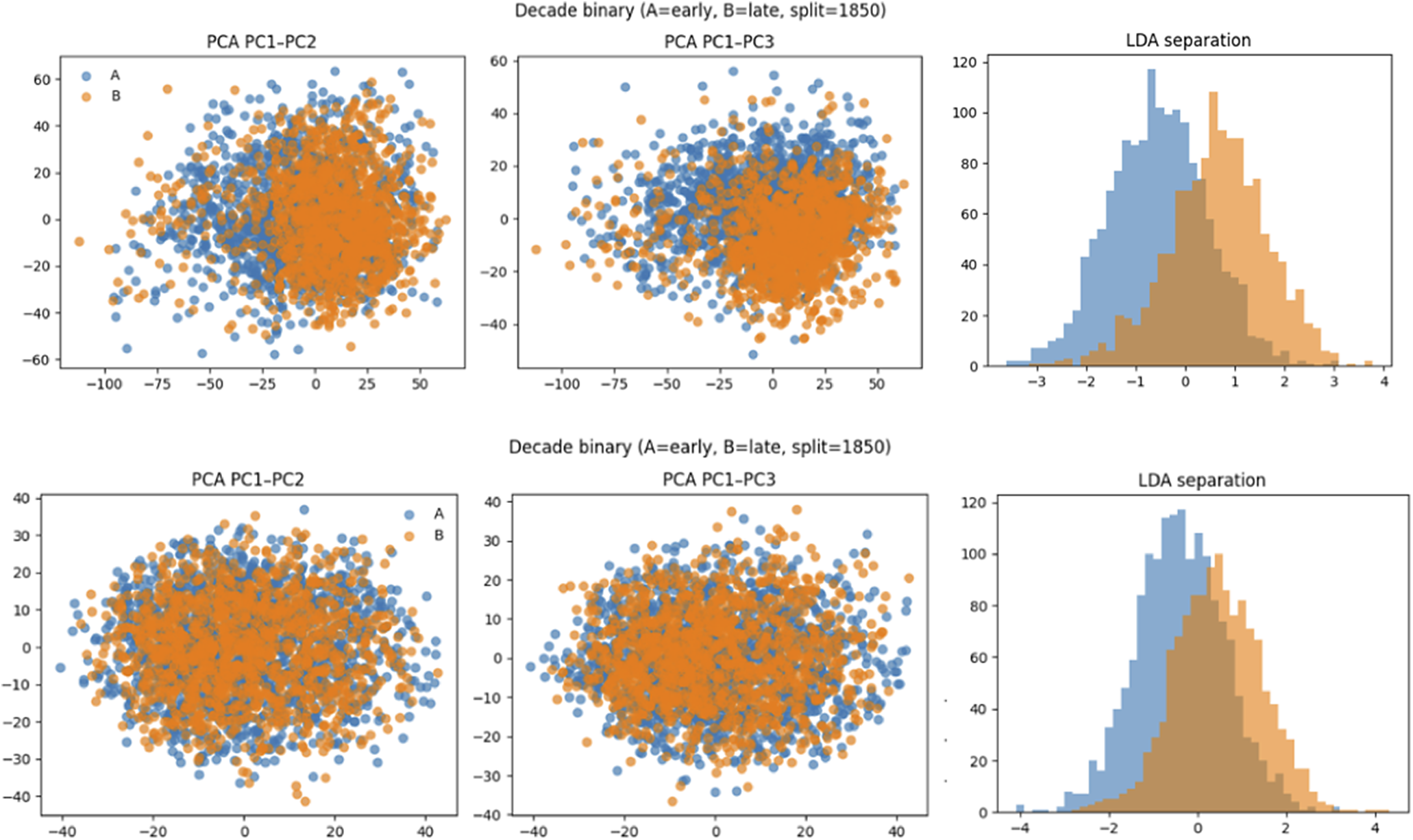


 Open access


Rapid Responses
No Rapid Responses have been published for this article.