





Impact Statement
The work in this article provides sensor placement optimization strategies bringing the possibility of sensor failure and backup sensors into consideration, for wired sensor systems. The focus is on optimization for modal identification or damage identification. The sensor deployments obtained can provide excellent performance when all sensors are working normally and guarantee good performance when partial sensors fail. Furthermore, it is shown that it is inadvisable to use backup sensors in wired sensor systems when the sensors are independent of each other.
1. Introduction
Sensor placement optimization (SPO) is a process of optimizing the number and location of sensors for a specific objective, to reduce instrument and processing costs without compromising the effect of monitoring. A statistical model is usually established to provide a quantitative objective function based on model parameters or the function of a model.
According to the assumptions of model parameters, that is, whether a prior is placed on the parameters, the notions of objective functions can be divided into classical and Bayesian ones. Kammer (Reference Kammer1991) and Yao et al. (Reference Yao, Sethares and Kammer1993) used a linear model to describe the relationship between sensor outputs and target mode shapes and optimized sensor combinations to maximize estimation quality of target modal coordinates. The difference between the classical optimization objectives adopted by Kammer (Reference Kammer1991) and Yao et al. (Reference Yao, Sethares and Kammer1993) is the scalarization approach of the covariance of variable errors. Further studies of mode shape-based SPO, taking into account modeling errors and measurement noise, can be found in Kammer (Reference Kammer1992a,b) and Jaya et al. (Reference Jaya, Ceravolo, Fragonara and Matta2020). Objective functions may use quantities in information theory, such as entropy and mutual information, or may use concepts from Bayesian statistics. Papadimitriou (Reference Papadimitriou2004) parameterized a structural model to describe the input–output behavior of a structure, and information entropy was used to measure uncertainty of the parameters updated by the measurements from a set of sensors. The sensor combination corresponding to the smallest entropy, in other words, the smallest uncertainty of the estimated parameters, was chosen as the optimal result. Krause et al. (Reference Krause, Singh and Guestrin2008) took a model used in spatial statistics—a Gaussian process—and used mutual information to measure the effect of selected sensors on the predictive uncertainty of variables in unobserved locations, so that the prediction quality over the whole space of interest was considered. In this case, the sensor combination corresponding to the largest mutual information, or rather to the maximum reduction in the uncertainty of responses from unobserved locations, was chosen as the optimal one.
When it comes to optimization objectives using a model function as the basis, most of them are related to supervised approaches, in which data for different structural states are involved to train a model. Worden and Burrows (Reference Worden and Burrows2001) adopted an established supervised learning algorithm—a neural network—to rank a structural health monitoring (SHM) sensor layout according to the normalized mean-square error between the desired responses and estimated responses and probability of misclassification. The sensor deployment with the minimum weighted fitness value was treated as the optimal result. Considering the ability to classify a large amount of multivariate data, Eshghi et al. (Reference Eshghi, Lee, Jung and Wang2019) used a Mahalanobis distance classifier to carry out the reliability-based sensor system design to minimize the area of sensor patches while satisfying the detectability requirement for different health states. If a prior is placed on the probability of the potential outcomes of various structural states, the Bayes risk can be used as an objective function to minimize the cost of each outcome, which is demonstrated in Flynn and Todd (Reference Flynn and Todd2010).
Some comprehensive references on SPO for SHM are available in Ostachowicz et al. (Reference Ostachowicz, Soman and Malinowski2019), Barthorpe and Worden (Reference Barthorpe and Worden2020), and Tan and Zhang (Reference Tan and Zhang2020) and Barthorpe and Worden (Reference Barthorpe and Worden2020). Ostachowicz et al. (Reference Ostachowicz, Soman and Malinowski2019) discuss the optimisation objective functions corresponding to each SHM technique more systematically, by dividing the SHM techniques into three types. Tan and Zhang (Reference Tan and Zhang2020) put more effort into classifying and comparing the optimisation algorithms, which are treated as consisting of five different types. In particular, the development of evolutionary optimisation methodologies and sequential sensor placement algorithms is clearly illustrated. Barthorpe and Worden (Reference Barthorpe and Worden2020) provide a more complete demonstration of optimisation objectives and specify emerging trends and future directions of SHM SPO.
The scope of the current article belongs to the classical optimization criteria based on model parameters. However, except for the traditional objective functions based on mode shapes, a predefined criterion based on canonical correlations, originally developed by Hotelling (Reference Hotelling1936), is firstly used to evaluate a sensor layout, which can transfer the function of linear discriminant analysis into the parameter estimation issue (Sun and Chen, Reference Sun and Chen2007). One reason for using this criterion is that it is usually more computationally efficient than criteria depending on model training. In existing research, correlation-based criteria have been widely applied in feature selection (Hall, Reference Hall1999; Yu and Liu, Reference Yu and Liu2003; Zhang and Lang, Reference Zhang and Lang2022), and some efforts have been made to extend its application to the SPO field. Chen et al. (Reference Chen, Bao, Tang, Chen and Li2020) defined a coefficient to quantify the geometric correlation of probability distributions of data collected by pairs of sensors. Sensor pairs with larger correlation indexes were selected to provide the data for predicting the shapes of all probability density functions. However, the redundancy and interaction of information from different sensors were not considered in this article. Lu et al. (Reference Lu, Wen, Teng, Li and Li2016) narrowed the range of sensor selection by maximizing the coefficient based on a correlation matrix and then minimized the correlation of the data provided by these candidate sensors to determine the final optimization result, but still ignored the information interaction. In contrast, the criteria based on canonical correlations can inherently take account of the information redundancy and interaction (Hall, Reference Hall1999; Zhang and Lang, Reference Zhang and Lang2022), which is another reason for using this kind of criterion as an optimization objective in this article.
In addition, sensor failures may seriously affect the overall performance of the sensor system, especially when sensors that collect unique and critical information fail; therefore, it is necessary to study the optimization of sensor systems that consider the effects of sensor failures. For wired sensor networks, Side et al. (Reference Side, Staszewski, Wardle and Worden1997) developed a novel optimization idea for fail-safe sensor distributions. By maximizing the worst performance of $ N-1 $
-sensor distributions generated by an
$ N-1 $
-sensor distributions generated by an $ N $
-sensor distribution, this optimization approach can provide a sensor set that can maintain an acceptable level of damage identification performance after a sensor failure. However, the objective function was only composed of the child fitness, which led to a conflict between the fail-safe mother distribution and optimal mother distribution. In this article, the improved fail-safe optimization method will be proposed to comprehensively consider the fitness of the mother distribution and worst sub-distribution for modal identification and damage identification.
$ N $
-sensor distribution, this optimization approach can provide a sensor set that can maintain an acceptable level of damage identification performance after a sensor failure. However, the objective function was only composed of the child fitness, which led to a conflict between the fail-safe mother distribution and optimal mother distribution. In this article, the improved fail-safe optimization method will be proposed to comprehensively consider the fitness of the mother distribution and worst sub-distribution for modal identification and damage identification.
For wireless sensor networks, Bhuiyan et al. (Reference Bhuiyan, Wang, Cao and Wu2013) proposed a backup or redundant sensor placement algorithm by incorporating the requirements of SHM and the limitations of wireless sensor networks to ensure a given level of fault tolerance. The case study showed that if the effects of sensor failures were not handled properly, it is meaningless to apply wireless sensor networks to SHM. Note that, for wireless sensor networks, sensor nodes within a sensor field will cooperate along designed routes through wireless connections, to transmit data to the base station; therefore, the failure of one sensor may affect the acquisition of data from other sensors. More information about wireless sensors and the wireless SPO can be found in Iqbal et al. (Reference Iqbal, Naeem, Anpalagan, Ahmed and Azam2015) and Abdollahzadeh and Navimipour (Reference Abdollahzadeh and Navimipour2016). Therefore, for the wireless sensor network, except the effects of sensor failures, solutions to deal with failures, such as placing backup sensors, must be considered during optimization, as demonstrated by Bhuiyan et al. (Reference Bhuiyan, Wang, Cao and Wu2013). This article assumes a wired sensor network where the failure of each sensor will not affect the data acquisition of other sensors and discusses whether it is worthwhile to design a sensor network with redundant sensors. Here, sensor failure refers to a situation where the sensor fails to provide any usable information, regardless of whether it is damaged or unable to connect to the network. Since the main task of this article is to evaluate whether the effects or the countermeasures of sensor failures need to be considered in the optimization process, how to evaluate whether the sensor is damaged is beyond the scope of this current article.
The major novelties of this article include:
-
1. This article studies the sensor location optimization algorithm considering sensor failure for both modal identification and damage identification. It is worth mentioning that the objective function for damage identification is based on canonical correlation analysis, which is the first use for SPO.
-
2. The optimization process of the fail-safe sensor distribution is improved. In addition to considering the performance of sensor distributions after sensor failure, the performance of the initial distribution is also integrated into the optimization process.
-
3. An optimization concept for the distribution of fail-safe redundant sensors is proposed. In the optimization design of the wired sensor deployment, the solution to deal with the failed sensor is considered, and then the value of this solution is discussed.
-
4. The approach is validated on a real structure, a full wing of a glider aircraft.
The article is organized as follows: the next section introduces the theoretical basis of the four optimization objectives belonging to two types of optimization purposes. Section 3 demonstrates the optimization flow to obtain fail-safe sensor distributions and fail-safe distributions with redundancy. Section 4 describes the tests on a glider wing to provide data for the case study. A series of results are presented and discussed in Section 5. The article is summarized at the end.
2. Optimization Objectives
The optimization objectives used for SPO depend on the purpose of the system and include the determinant of the Fisher information matrix (DFIM), the DFIM weighted by average-driving-point residue (DFIM-ADPR), the sum of squared canonical correlation coefficients (SSC), and the SSC weighted by average-driving-point residue (SSC-ADPR). The first two objectives, developed by Yao et al. (Reference Yao, Sethares and Kammer1993) and Imamovic and Ewins (Reference Imamovic and Ewins1997), are widely used in SPO tasks, but the last two objectives are used for SPO for the first time. These objectives are selected or proposed from three perspectives, including the accuracy of the target modal-coordinate estimate, the vibration energy, and the information on the damage of interest. The detailed introduction is as follows.
2.1. Determinant of the Fisher information matrix
For the modal identification task, assume that there are limited candidate sensor locations and $ J $
modes to be identified. Suppose
$ J $
modes to be identified. Suppose $ I $
sensors will be selected from the candidate sensors. The project budget determines the maximum value of
$ I $
sensors will be selected from the candidate sensors. The project budget determines the maximum value of $ I $
. For the
$ I $
. For the $ s\mathrm{th} $
combination of the
$ s\mathrm{th} $
combination of the $ I $
sensor locations, the outputs of these chosen sensors are described by a vector
$ I $
sensor locations, the outputs of these chosen sensors are described by a vector $ {\mathbf{y}}_s\in {\mathrm{\mathbb{R}}}^{I\times 1} $
, which is given by,
$ {\mathbf{y}}_s\in {\mathrm{\mathbb{R}}}^{I\times 1} $
, which is given by,
 $$ {\mathbf{y}}_s\hskip0.35em =\hskip0.35em {\boldsymbol{\Phi}}_s{\mathbf{q}}_s+{\varepsilon}_s $$
where $ {\boldsymbol{\Phi}}_s\in {\mathrm{\mathbb{R}}}^{I\times J} $
is the
$ {\boldsymbol{\Phi}}_s\in {\mathrm{\mathbb{R}}}^{I\times J} $
is the $ s\mathrm{th} $
target modal matrix,
$ s\mathrm{th} $
target modal matrix, $ {\mathbf{q}}_s\in {\mathrm{\mathbb{R}}}^{J\times 1} $
is the vector of the target modal coordinates, and
$ {\mathbf{q}}_s\in {\mathrm{\mathbb{R}}}^{J\times 1} $
is the vector of the target modal coordinates, and $ {\varepsilon}_s\in {\mathrm{\mathbb{R}}}^{I\times 1} $
is the vector of measurement noise at these selected sensors, which is assumed to be zero-mean Gaussian noise. The least-squares estimate of the target modal coordinates for the
$ {\varepsilon}_s\in {\mathrm{\mathbb{R}}}^{I\times 1} $
is the vector of measurement noise at these selected sensors, which is assumed to be zero-mean Gaussian noise. The least-squares estimate of the target modal coordinates for the $ s\mathrm{th} $
sensor combination can be acquired from,
$ s\mathrm{th} $
sensor combination can be acquired from,
 $$ {\hat{\mathbf{q}}}_s\hskip0.35em =\hskip0.35em {\left({\boldsymbol{\Phi}}_s^{\top }{\boldsymbol{\Phi}}_s\right)}^{-1}{\boldsymbol{\Phi}}_s^{\top }{\mathbf{y}}_s $$
It can be seen that $ I $
should not be less than
$ I $
should not be less than $ J $
to make
$ J $
to make $ {\boldsymbol{\Phi}}_s $
invertible.
$ {\boldsymbol{\Phi}}_s $
invertible.
According to Beck and Arnold (Reference Beck and Arnold1977), it can be assumed that the probability density function of $ {\hat{\mathbf{q}}}_s $
is Gaussian, and the corresponding confidence region can be treated as the interior of the hyperellipsoid,
$ {\hat{\mathbf{q}}}_s $
is Gaussian, and the corresponding confidence region can be treated as the interior of the hyperellipsoid,
 $$ {\left({\hat{\mathbf{q}}}_s-{\mathbf{q}}_s\right)}^{\top }{{\mathbf{F}}_{\hat{\mathbf{q}}}}_s^{-1}\left({\hat{\mathbf{q}}}_s-{\mathbf{q}}_s\right)\hskip0.35em =\hskip0.35em {c}^2 $$
where $ {\mathbf{F}}_{{\hat{\mathbf{q}}}_{\mathbf{s}}}\hskip0.35em =\hskip0.35em {\left({\boldsymbol{\Phi}}_s^{\top }{\boldsymbol{\Phi}}_s\right)}^{-1}{\boldsymbol{\Phi}}_s^{\top}\mathbf{E}\left({\varepsilon}_s{\varepsilon}_s^{\top}\right){\boldsymbol{\Phi}}_s{\left({\boldsymbol{\Phi}}_s^{\top }{\boldsymbol{\Phi}}_s\right)}^{-1} $
is the covariance matrix of the estimation error of
$ {\mathbf{F}}_{{\hat{\mathbf{q}}}_{\mathbf{s}}}\hskip0.35em =\hskip0.35em {\left({\boldsymbol{\Phi}}_s^{\top }{\boldsymbol{\Phi}}_s\right)}^{-1}{\boldsymbol{\Phi}}_s^{\top}\mathbf{E}\left({\varepsilon}_s{\varepsilon}_s^{\top}\right){\boldsymbol{\Phi}}_s{\left({\boldsymbol{\Phi}}_s^{\top }{\boldsymbol{\Phi}}_s\right)}^{-1} $
is the covariance matrix of the estimation error of $ {\hat{\mathbf{q}}}_s $
and
$ {\hat{\mathbf{q}}}_s $
and $ c $
is a constant related to the confidence level. The volume
$ c $
is a constant related to the confidence level. The volume $ {D}_s $
of the hyperellipsoid can be obtained by Yao et al. (Reference Yao, Sethares and Kammer1993),
$ {D}_s $
of the hyperellipsoid can be obtained by Yao et al. (Reference Yao, Sethares and Kammer1993),
 $$ {D}_s\hskip0.35em =\hskip0.35em {\pi}^{I/2}{c}^I{\left[\det \left({\mathbf{F}}_{\hat{\mathbf{q}}s}\right)\right]}^{1/2}{\left[\boldsymbol{\Gamma} \left(I/2+1\right)\right]}^{-1} $$
where $ \boldsymbol{\Gamma} \left(\cdot \right) $
refers to the gamma function and
$ \boldsymbol{\Gamma} \left(\cdot \right) $
refers to the gamma function and $ \det \left(\cdot \right) $
refers to the determinant. To obtain the best linear unbiased estimator, that is, the most accurate estimation of the target modal coordinates, the volume of this confidence region should be minimized. Because
$ \det \left(\cdot \right) $
refers to the determinant. To obtain the best linear unbiased estimator, that is, the most accurate estimation of the target modal coordinates, the volume of this confidence region should be minimized. Because $ {\mathbf{F}}_{{\hat{\mathbf{q}}}_{\mathbf{s}}} $
is the only variable in Equation (4), the key to the optimization problem is to minimize the determinant of
$ {\mathbf{F}}_{{\hat{\mathbf{q}}}_{\mathbf{s}}} $
is the only variable in Equation (4), the key to the optimization problem is to minimize the determinant of $ {\mathbf{F}}_{{\hat{\mathbf{q}}}_{\mathbf{s}}} $
. As it was assumed that the measurement noise of sensors was uncorrelated and of equal variance
$ {\mathbf{F}}_{{\hat{\mathbf{q}}}_{\mathbf{s}}} $
. As it was assumed that the measurement noise of sensors was uncorrelated and of equal variance $ {\sigma}^2 $
in Yao et al. (Reference Yao, Sethares and Kammer1993), they showed that,
$ {\sigma}^2 $
in Yao et al. (Reference Yao, Sethares and Kammer1993), they showed that,
 $$ {\displaystyle \begin{array}{ll}\det \left({\mathbf{F}}_{{\hat{\mathbf{q}}}_{\mathbf{s}}}\right)& \hskip0.35em =\hskip0.35em \det \left[{\sigma}^2{\left({\boldsymbol{\Phi}}_s^{\top }{\boldsymbol{\Phi}}_s\right)}^{-1}\right]\\ {}& \hskip0.35em =\hskip0.35em {\sigma}^{2I}\det {\left[\left({\boldsymbol{\Phi}}_s^{\top }{\boldsymbol{\Phi}}_s\right)\right]}^{-1}\end{array}} $$
Because the $ {{\mathbf{F}}_{{\hat{\mathbf{q}}}_{\mathbf{s}}}}^{-1} $
was defined as the Fisher information matrix (FIM) in Middleton (Reference Middleton1996),
$ {{\mathbf{F}}_{{\hat{\mathbf{q}}}_{\mathbf{s}}}}^{-1} $
was defined as the Fisher information matrix (FIM) in Middleton (Reference Middleton1996), $ {\boldsymbol{\Phi}}_s^{\top }{\boldsymbol{\Phi}}_s $
was subsequently referred to as the FIM in Kammer (Reference Kammer1991). Thus, minimizing the determinant of
$ {\boldsymbol{\Phi}}_s^{\top }{\boldsymbol{\Phi}}_s $
was subsequently referred to as the FIM in Kammer (Reference Kammer1991). Thus, minimizing the determinant of $ {\mathbf{F}}_{{\hat{\mathbf{q}}}_{\mathbf{s}}} $
, as discussed earlier, is equivalent to maximizing the DFIM, that is, maximizing
$ {\mathbf{F}}_{{\hat{\mathbf{q}}}_{\mathbf{s}}} $
, as discussed earlier, is equivalent to maximizing the DFIM, that is, maximizing $ \det \left({\boldsymbol{\Phi}}_s^{\top }{\boldsymbol{\Phi}}_s\right) $
. Note that when the lower-upper (LU) decomposition is applied, the computational complexity of calculating the DFIM is
$ \det \left({\boldsymbol{\Phi}}_s^{\top }{\boldsymbol{\Phi}}_s\right) $
. Note that when the lower-upper (LU) decomposition is applied, the computational complexity of calculating the DFIM is $ \mathcal{O}\left({J}^3\right) $
. Based on this, the FIM-based criterion can be applied to compare the different sensor combinations with the same number of sensors to find the optimal sensor deployment that is most beneficial to estimate the target modal coordinates most accurately.
$ \mathcal{O}\left({J}^3\right) $
. Based on this, the FIM-based criterion can be applied to compare the different sensor combinations with the same number of sensors to find the optimal sensor deployment that is most beneficial to estimate the target modal coordinates most accurately.
2.2. DFIM average driving-point residue
There is an obvious disadvantage of using the DFIM as an optimization objective, in that sensor locations with low signal strength can be selected. In order to overcome this issue and improve the signal-to-noise ratio, the ADPR can be combined with the DFIM to give the $ \det {\left({\boldsymbol{\Phi}}_s^{\top }{\boldsymbol{\Phi}}_s\right)}_{\mathrm{ADPR}} $
corresponding to one sensor combination (Imamovic and Ewins, Reference Imamovic and Ewins1997), which is defined as,
$ \det {\left({\boldsymbol{\Phi}}_s^{\top }{\boldsymbol{\Phi}}_s\right)}_{\mathrm{ADPR}} $
corresponding to one sensor combination (Imamovic and Ewins, Reference Imamovic and Ewins1997), which is defined as,
 $$ \det {\left({\boldsymbol{\Phi}}_s^{\top }{\boldsymbol{\Phi}}_s\right)}_{\mathrm{ADPR}}\hskip0.35em =\hskip0.35em \det \left({\boldsymbol{\Phi}}_s^{\top }{\boldsymbol{\Phi}}_s\right)\sum \limits_{i\hskip0.35em =\hskip0.35em 1}^I\sum \limits_{j\hskip0.35em =\hskip0.35em 1}^J\frac{{\left({\phi}_s^{ij}\right)}^2}{\omega_j} $$
where $ {\phi}_s^{ij} $
is the entry corresponding to the
$ {\phi}_s^{ij} $
is the entry corresponding to the $ i\mathrm{th} $
degree of freedom of the
$ i\mathrm{th} $
degree of freedom of the $ j\mathrm{th} $
target mode in the
$ j\mathrm{th} $
target mode in the $ s\mathrm{th} $
target modal matrix and
$ s\mathrm{th} $
target modal matrix and $ {\omega}_j $
is the natural frequency corresponding to the
$ {\omega}_j $
is the natural frequency corresponding to the $ j\mathrm{th} $
target mode. This criterion, the DFIM–ADPR, should be maximized to find the optimal sensor deployment.
$ j\mathrm{th} $
target mode. This criterion, the DFIM–ADPR, should be maximized to find the optimal sensor deployment.
2.3. Sum of squared canonical correlation coefficients
For the damage identification task, to make the sensor system have good performance in identifying certain damage states of concern, information about these high-potential failures should be included in the sensor system optimization process. These damage states can be determined by conducting failure mode analysis and referring to historical data about damage states collected on the existing structures.
The SSC is used here as a criterion to measure the maximal linear association between two co-occurring multivariate random variables with $ K $
observations, which are collected as matrices
$ K $
observations, which are collected as matrices $ \mathbf{X}\in {\mathrm{\mathbb{R}}}^{K\times M} $
and
$ \mathbf{X}\in {\mathrm{\mathbb{R}}}^{K\times M} $
and $ \mathbf{Y}\in {\mathrm{\mathbb{R}}}^{K\times N} $
(Hotelling, Reference Hotelling1936). In this article, a matrix
$ \mathbf{Y}\in {\mathrm{\mathbb{R}}}^{K\times N} $
(Hotelling, Reference Hotelling1936). In this article, a matrix $ \mathbf{X} $
represents the
$ \mathbf{X} $
represents the $ K $
samples of
$ K $
samples of $ M $
features. A matrix
$ M $
features. A matrix $ \mathbf{Y} $
refers to labels represented by
$ \mathbf{Y} $
refers to labels represented by $ N $
variables associated with each sample. This criterion can help to directly measure the effectiveness of data for predicting structural states to a certain extent, without the need for model training. Furthermore, since a set of features in
$ N $
variables associated with each sample. This criterion can help to directly measure the effectiveness of data for predicting structural states to a certain extent, without the need for model training. Furthermore, since a set of features in $ \mathbf{X} $
are evaluated together, rather than evaluating each feature individually, the interaction of features can be considered, avoiding redundant features.
$ \mathbf{X} $
are evaluated together, rather than evaluating each feature individually, the interaction of features can be considered, avoiding redundant features.
The acquisition of the SSC can be realized by finding pairs of projection directions $ \mathbf{U}\in {\mathrm{\mathbb{R}}}^{M\times L} $
and
$ \mathbf{U}\in {\mathrm{\mathbb{R}}}^{M\times L} $
and $ \mathbf{V}\in {\mathrm{\mathbb{R}}}^{N\times L} $
, so that the Pearson’s correlation coefficient between
$ \mathbf{V}\in {\mathrm{\mathbb{R}}}^{N\times L} $
, so that the Pearson’s correlation coefficient between $ {\mathbf{X}}_{\mathrm{C}}{\mathbf{u}}_l $
and
$ {\mathbf{X}}_{\mathrm{C}}{\mathbf{u}}_l $
and $ {\mathbf{Y}}_{\mathrm{C}}{\mathbf{v}}_l $
for the
$ {\mathbf{Y}}_{\mathrm{C}}{\mathbf{v}}_l $
for the $ l\mathrm{th} $
pair of projection directions is maximized (Zhang and Lang, Reference Zhang and Lang2022), that is,
$ l\mathrm{th} $
pair of projection directions is maximized (Zhang and Lang, Reference Zhang and Lang2022), that is,
 $$ {\displaystyle \begin{array}{ll}{R}_l\left(\mathbf{X},\mathbf{Y}\right)& \triangleq \underset{{\mathbf{u}}_l,{\mathbf{v}}_l}{\max }r\left({\mathbf{X}\mathbf{u}}_l,{\mathbf{Y}\mathbf{v}}_l\right)\\ {}& \triangleq \underset{{\mathbf{u}}_l,{\mathbf{v}}_l}{\max}\frac{{\mathbf{u}}_l^{\top }{\mathbf{X}}_{\mathrm{C}}^{\top }{\mathbf{Y}}_{\mathrm{C}}{\mathbf{v}}_l}{\sqrt{{\mathbf{u}}_l^{\top }{\mathbf{X}}_{\mathrm{C}}^{\top }{\mathbf{X}}_{\mathrm{C}}{\mathbf{u}}_l}\sqrt{{\mathbf{v}}_l^{\top }{\mathbf{Y}}_{\mathrm{C}}^{\top }{\mathbf{Y}}_{\mathrm{C}}{\mathbf{v}}_l}}\end{array}} $$
where $ {\mathbf{X}}_{\mathrm{C}}\hskip0.35em =\hskip0.35em \mathbf{X}-\overline{\mathbf{X}} $
and
$ {\mathbf{X}}_{\mathrm{C}}\hskip0.35em =\hskip0.35em \mathbf{X}-\overline{\mathbf{X}} $
and $ {\mathbf{Y}}_{\mathrm{C}}\hskip0.35em =\hskip0.35em \mathbf{Y}-\overline{\mathbf{Y}} $
.
$ {\mathbf{Y}}_{\mathrm{C}}\hskip0.35em =\hskip0.35em \mathbf{Y}-\overline{\mathbf{Y}} $
. $ \overline{\mathbf{X}} $
and
$ \overline{\mathbf{X}} $
and $ \overline{\mathbf{Y}} $
are the means of columns of
$ \overline{\mathbf{Y}} $
are the means of columns of $ \mathbf{X} $
and
$ \mathbf{X} $
and $ \mathbf{Y} $
, respectively.
$ \mathbf{Y} $
, respectively. $ R\left(\cdot \right) $
refers to the canonical correlation coefficient and
$ R\left(\cdot \right) $
refers to the canonical correlation coefficient and $ r\left(\cdot \right) $
refers to the Pearson’s correlation coefficient. It can be seen that
$ r\left(\cdot \right) $
refers to the Pearson’s correlation coefficient. It can be seen that $ {R}_l\left(\mathbf{X},\mathbf{Y}\right) $
does not depend on the scale of
$ {R}_l\left(\mathbf{X},\mathbf{Y}\right) $
does not depend on the scale of $ {\mathbf{u}}_l $
and
$ {\mathbf{u}}_l $
and $ {\mathbf{v}}_l $
. Therefore, the
$ {\mathbf{v}}_l $
. Therefore, the $ {\mathbf{Xu}}_l $
and
$ {\mathbf{Xu}}_l $
and $ {\mathbf{Yv}}_l $
can be standardized to have unit variance. Then, Equation (7) can be expressed as,
$ {\mathbf{Yv}}_l $
can be standardized to have unit variance. Then, Equation (7) can be expressed as,
 $$ \underset{{\mathbf{u}}_l,{\mathbf{v}}_l}{\max }{\mathbf{u}}_l^{\top }{\mathbf{X}}_{\mathrm{C}}^{\top }{\mathbf{Y}}_{\mathrm{C}}{\mathbf{v}}_l,\hskip1em s.t.\hskip0.2em {\mathbf{u}}_l^{\top }{\mathbf{X}}_{\mathrm{C}}^{\top }{\mathbf{X}}_{\mathrm{C}}{\mathbf{u}}_l\hskip0.35em =\hskip0.35em 1,{\mathbf{v}}_l^{\top }{\mathbf{Y}}_{\mathrm{C}}^{\top }{\mathbf{Y}}_{\mathrm{C}}{\mathbf{v}}_l\hskip0.35em =\hskip0.35em 1 $$
Lagrange multipliers $ \alpha $
and
$ \alpha $
and $ \beta $
can be used to find
$ \beta $
can be used to find $ {\mathbf{u}}_l $
and
$ {\mathbf{u}}_l $
and $ {\mathbf{v}}_l $
, such that,
$ {\mathbf{v}}_l $
, such that,
 $$ F\left({\mathbf{u}}_l,{\mathbf{v}}_l\right)\hskip0.35em =\hskip0.35em {\mathbf{u}}_l^{\top }{\mathbf{X}}_{\mathrm{C}}^{\top }{\mathbf{Y}}_{\mathrm{C}}{\mathbf{v}}_l-\frac{1}{2}\alpha \left({\mathbf{u}}_l^{\top }{\mathbf{X}}_{\mathrm{C}}^{\top }{\mathbf{X}}_{\mathrm{C}}{\mathbf{u}}_l-1\right)-\frac{1}{2}\beta \left({\mathbf{v}}_l^{\top }{\mathbf{Y}}_{\mathrm{C}}^{\top }{\mathbf{Y}}_{\mathrm{C}}{\mathbf{v}}_l-1\right) $$
followed by,
 $$ \frac{\mathrm{d}}{\mathrm{d}{\mathbf{u}}_l}\left(F\left({\mathbf{u}}_l,{\mathbf{v}}_l\right)\right)\hskip0.35em =\hskip0.35em {\mathbf{X}}_{\mathrm{C}}^{\top }{\mathbf{Y}}_{\mathrm{C}}{\mathbf{v}}_l-\alpha {\mathbf{X}}_{\mathrm{C}}^{\top }{\mathbf{X}}_{\mathrm{C}}{\mathbf{u}}_l\hskip0.35em =\hskip0.35em \mathbf{0} $$
 $$ \frac{\mathrm{d}}{\mathrm{d}{\mathbf{v}}_l}\left(F\left({\mathbf{u}}_l,{\mathbf{v}}_l\right)\right)\hskip0.35em =\hskip0.35em {\mathbf{X}}_{\mathrm{C}}^{\top }{\mathbf{Y}}_{\mathrm{C}}{\mathbf{u}}_l-\beta {\mathbf{Y}}_{\mathrm{C}}^{\top }{\mathbf{Y}}_{\mathrm{C}}{\mathbf{v}}_l\hskip0.35em =\hskip0.35em \mathbf{0} $$
Premultiplying Equations (10) and (11) by $ {\mathbf{u}}_l^{\top } $
and
$ {\mathbf{u}}_l^{\top } $
and $ {\mathbf{v}}_l^{\top } $
respectively, gives
$ {\mathbf{v}}_l^{\top } $
respectively, gives
 $$ {\mathbf{u}}_l^{\top }{\mathbf{X}}_{\mathrm{C}}^{\top }{\mathbf{Y}}_{\mathrm{C}}{\mathbf{v}}_l-\alpha {\mathbf{u}}_l^{\top }{\mathbf{X}}_{\mathrm{C}}^{\top }{\mathbf{X}}_{\mathrm{C}}{\mathbf{u}}_l\hskip0.35em =\hskip0.35em \mathbf{0} $$
 $$ {\mathbf{v}}_l^{\top }{\mathbf{X}}_{\mathrm{C}}^{\top }{\mathbf{Y}}_{\mathrm{C}}{\mathbf{u}}_l-\beta {\mathbf{v}}_l^{\top }{\mathbf{Y}}_{\mathrm{C}}^{\top }{\mathbf{Y}}_{\mathrm{C}}{\mathbf{v}}_l\hskip0.35em =\hskip0.35em \mathbf{0} $$
It can be found that $ {R}_l\left(\mathbf{X},\mathbf{Y}\right)\hskip0.35em =\hskip0.35em \alpha \hskip0.35em =\hskip0.35em \beta $
.
$ {R}_l\left(\mathbf{X},\mathbf{Y}\right)\hskip0.35em =\hskip0.35em \alpha \hskip0.35em =\hskip0.35em \beta $
.
By a series of transformations based on Equations (10) and (11), the values of $ R\left(\mathbf{X},\mathbf{Y}\right) $
can be obtained by solving the eigenvalue equations given by Hardoon et al. (Reference Hardoon, Szedmak and Shawe-Taylor2004) and Cox (Reference Cox2005),
$ R\left(\mathbf{X},\mathbf{Y}\right) $
can be obtained by solving the eigenvalue equations given by Hardoon et al. (Reference Hardoon, Szedmak and Shawe-Taylor2004) and Cox (Reference Cox2005),
 $$ \left[{\left({\mathbf{X}}_{\mathrm{C}}^{\top }{\mathbf{X}}_{\mathrm{C}}\right)}^{-1}{\mathbf{X}}_{\mathrm{C}}^{\top }{\mathbf{Y}}_{\mathrm{C}}{\left({\mathbf{Y}}_{\mathrm{C}}^{\top }{\mathbf{Y}}_{\mathrm{C}}\right)}^{-1}{\mathbf{Y}}_{\mathrm{C}}^{\top }{\mathbf{X}}_{\mathrm{C}}-{R}_l^2\Big(\mathbf{X},\mathbf{Y}\Big)\mathbf{I}\right]{\mathbf{u}}_l\hskip0.35em =\hskip0.35em \mathbf{0} $$
 $$ \left[{\left({\mathbf{Y}}_{\mathrm{C}}^{\top }{\mathbf{Y}}_{\mathrm{C}}\right)}^{-1}{\mathbf{Y}}_{\mathrm{C}}^{\top }{\mathbf{X}}_{\mathrm{C}}{\left({\mathbf{X}}_{\mathrm{C}}^{\top }{\mathbf{X}}_{\mathrm{C}}\right)}^{-1}{\mathbf{X}}_{\mathrm{C}}^{\top }{\mathbf{Y}}_{\mathrm{C}}-{R}_l^2\Big(\mathbf{X},\mathbf{Y}\Big)\mathbf{I}\right]{\mathbf{v}}_l\hskip0.35em =\hskip0.35em \mathbf{0} $$
The corresponding projection directions $ {\mathbf{u}}_l\in {\mathrm{\mathbb{R}}}^{M\times 1} $
and
$ {\mathbf{u}}_l\in {\mathrm{\mathbb{R}}}^{M\times 1} $
and $ {\mathbf{v}}_l\in {\mathrm{\mathbb{R}}}^{N\times 1} $
are also obtained now. Since
$ {\mathbf{v}}_l\in {\mathrm{\mathbb{R}}}^{N\times 1} $
are also obtained now. Since $ {R}_l\left(\mathbf{X},\mathbf{Y}\right) $
ranges between −1 and 1, the eigenvalue
$ {R}_l\left(\mathbf{X},\mathbf{Y}\right) $
ranges between −1 and 1, the eigenvalue $ {R}_l^2\left(\mathbf{X},\mathbf{Y}\right) $
takes values between 0 and 1. If
$ {R}_l^2\left(\mathbf{X},\mathbf{Y}\right) $
takes values between 0 and 1. If $ {\mathbf{X}}_{\mathrm{C}} $
and
$ {\mathbf{X}}_{\mathrm{C}} $
and $ {\mathbf{Y}}_{\mathrm{C}} $
have full column rank, the number of the non-zero eigenvalues is not greater than
$ {\mathbf{Y}}_{\mathrm{C}} $
have full column rank, the number of the non-zero eigenvalues is not greater than $ \min \left(M,N\right) $
, that is, L is not greater than
$ \min \left(M,N\right) $
, that is, L is not greater than $ \min \left(M,N\right) $
.
$ \min \left(M,N\right) $
.
On this basis, the sum of non-zero eigenvalues, that is, SSC, is adopted as a criterion for evaluating the effectiveness of a feature set from a sensor set to infer the structural state, which is given by,
 $$ {\displaystyle \begin{array}{ll}\sum \limits_{l\hskip0.35em =\hskip0.35em 1}^L{R}_l^2\left(\mathbf{X},\mathbf{Y}\right)& =\hskip0.35em \mathrm{tr}\left[{\left({\mathbf{X}}_{\mathrm{C}}^{\top }{\mathbf{X}}_{\mathrm{C}}\right)}^{-1}{\mathbf{X}}_{\mathrm{C}}^{\top }{\mathbf{Y}}_{\mathrm{C}}{\left({\mathbf{Y}}_{\mathrm{C}}^{\top }{\mathbf{Y}}_{\mathrm{C}}\right)}^{-1}{\mathbf{Y}}_{\mathrm{C}}^{\top }{\mathbf{X}}_{\mathrm{C}}\right]\\ {}& =\hskip0.35em \mathrm{tr}\left[{\left({\mathbf{Y}}_{\mathrm{C}}^{\top }{\mathbf{Y}}_{\mathrm{C}}\right)}^{-1}{\mathbf{Y}}_{\mathrm{C}}^{\top }{\mathbf{X}}_{\mathrm{C}}{\left({\mathbf{X}}_{\mathrm{C}}^{\top }{\mathbf{X}}_{\mathrm{C}}\right)}^{-1}{\mathbf{X}}_{\mathrm{C}}^{\top }{\mathbf{Y}}_{\mathrm{C}}\right]\end{array}} $$
where $ \mathrm{tr}\left[\cdot \right] $
represents the trace of a matrix. The computational complexity of Equation (15) is
$ \mathrm{tr}\left[\cdot \right] $
represents the trace of a matrix. The computational complexity of Equation (15) is $ \mathcal{O}\left({M}^2K\right) $
when
$ \mathcal{O}\left({M}^2K\right) $
when $ N\le M $
or
$ N\le M $
or $ \mathcal{O}\left({N}^2K\right) $
when
$ \mathcal{O}\left({N}^2K\right) $
when $ N>M $
. According to the SSC criterion, the optimal sensor deployment with the largest SSC among sensor combinations with the same number of sensors is conducive to the most accurate estimation of the structural labels because the features are more correlated with labels.
$ N>M $
. According to the SSC criterion, the optimal sensor deployment with the largest SSC among sensor combinations with the same number of sensors is conducive to the most accurate estimation of the structural labels because the features are more correlated with labels.
2.4. SSC average driving-point residue
If mode shapes are used as features for SPO with the aim of damage identification, the selected $ n $
mode shapes collected under different structural states can form a feature matrix
$ n $
mode shapes collected under different structural states can form a feature matrix $ {\mathbf{X}}_s\in {\mathrm{\mathbb{R}}}^{K\times \left(I\times J\right)} $
corresponding to the
$ {\mathbf{X}}_s\in {\mathrm{\mathbb{R}}}^{K\times \left(I\times J\right)} $
corresponding to the $ s\mathrm{th} $
combination of
$ s\mathrm{th} $
combination of $ I $
sensors. Rows refer to
$ I $
sensors. Rows refer to $ K $
observations for different healthy states, and columns refer to the relative displacement of
$ K $
observations for different healthy states, and columns refer to the relative displacement of $ I $
selected sensor locations on a structure in
$ I $
selected sensor locations on a structure in $ J $
modes. What is worth noting is that if only one mode shape is going to be considered, that is,
$ J $
modes. What is worth noting is that if only one mode shape is going to be considered, that is, $ J\hskip0.35em =\hskip0.35em 1 $
, the feature corresponding to
$ J\hskip0.35em =\hskip0.35em 1 $
, the feature corresponding to $ i\mathrm{th} $
sensor location will be a vector
$ i\mathrm{th} $
sensor location will be a vector $ {\mathbf{x}}_s^i\in {\mathrm{\mathbb{R}}}^{K\times 1} $
; if more than one mode shape is considered, that is,
$ {\mathbf{x}}_s^i\in {\mathrm{\mathbb{R}}}^{K\times 1} $
; if more than one mode shape is considered, that is, $ J>1 $
, the feature corresponding to
$ J>1 $
, the feature corresponding to $ i\mathrm{th} $
sensor location will be a matrix
$ i\mathrm{th} $
sensor location will be a matrix $ {\mathbf{X}}_s^i\in {\mathrm{\mathbb{R}}}^{K\times J} $
.
$ {\mathbf{X}}_s^i\in {\mathrm{\mathbb{R}}}^{K\times J} $
.
Similarly, the ADPR coefficient can be combined with SSC to improve the stability of the optimal sensor layout to noise, which is given by,
 $$ \sum \limits_{l\hskip0.35em =\hskip0.35em 1}^L{R}_l^2{\left(\mathbf{X},\mathbf{Y}\right)}_{\mathrm{ADPR}}\hskip0.35em =\hskip0.35em \sum \limits_{l\hskip0.35em =\hskip0.35em 1}^L{R}_l^2\left(\mathbf{X},\mathbf{Y}\right)\sum \limits_{k\hskip0.35em =\hskip0.35em 1}^K\sum \limits_{i\hskip0.35em =\hskip0.35em 1}^I\sum \limits_{j\hskip0.35em =\hskip0.35em 1}^J\frac{{\left({x}_s^{kij}\right)}^2}{\omega_j^k} $$
where $ {x}_s^{kij} $
is the entry corresponding to the
$ {x}_s^{kij} $
is the entry corresponding to the $ i\mathrm{th} $
degree of freedom of the
$ i\mathrm{th} $
degree of freedom of the $ j\mathrm{th} $
target mode from the
$ j\mathrm{th} $
target mode from the $ k\mathrm{th} $
observation of the
$ k\mathrm{th} $
observation of the $ s\mathrm{th} $
target modal matrix and
$ s\mathrm{th} $
target modal matrix and $ {\omega}_j^k $
is the natural frequency corresponding to the
$ {\omega}_j^k $
is the natural frequency corresponding to the $ j\mathrm{th} $
target mode in the
$ j\mathrm{th} $
target mode in the $ k\mathrm{th} $
observation. When the number of sensors is fixed, the sensor deployment with the largest SSC-ADPR will be considered the optimal sensor placement.
$ k\mathrm{th} $
observation. When the number of sensors is fixed, the sensor deployment with the largest SSC-ADPR will be considered the optimal sensor placement.
2.5. Discussion and handling of singular matrices
From Equations (5), (6), (15) and (16), it can be seen that these four optimization objectives are not applicable for the SPO with singular matrices, including the mode shape matrix ( $ \boldsymbol{\Phi} $
), the feature matrix (
$ \boldsymbol{\Phi} $
), the feature matrix ( $ \mathbf{X} $
), and the label matrix (
$ \mathbf{X} $
), and the label matrix ( $ \mathbf{Y} $
), which are not invertible. This means that it is necessary to check whether these matrices are singular before optimization using these four objectives.
$ \mathbf{Y} $
), which are not invertible. This means that it is necessary to check whether these matrices are singular before optimization using these four objectives.
Since the mode shapes are independent when the number of degrees of freedom is equal to or greater than the number of identified modes and the selected degrees of freedom are not centrally distributed, the singularity problem for a mode shape matrix ( $ \boldsymbol{\Phi} $
) can be solved by increasing the candidate sensor locations and changing the distribution of the candidate sensor locations. For the feature matrix (
$ \boldsymbol{\Phi} $
) can be solved by increasing the candidate sensor locations and changing the distribution of the candidate sensor locations. For the feature matrix ( $ \mathbf{X} $
), the sensor combination corresponding to a singular feature matrix can be discarded directly. Usually, the label matrix (
$ \mathbf{X} $
), the sensor combination corresponding to a singular feature matrix can be discarded directly. Usually, the label matrix ( $ \mathbf{Y} $
) is of full rank. If not, the redundant label information should be removed first.
$ \mathbf{Y} $
) is of full rank. If not, the redundant label information should be removed first.
3. Optimization Considering Sensor Failure and Sensor Redundancy
In order to make the performance of the sensor system less sensitive to sensor failures, two novel optimization ideas are proposed by combining the above optimization objectives with the effects of, or countermeasures to, sensor failures to obtain the fitness of sensor distribution.
The first approach, called the fail-safe sensor distribution, will take into account the effects of critical sensor failures when calculating the fitness of the sensor distribution. The second approach is called the fail-safe sensor distribution with redundancy, where the fitness results of the sensor distribution will be affected by the key critical failure handling scheme. The motivation for the second optimization idea is to explore, with a fixed number of sensors, a better strategy to place all sensors in different locations, to collect more information, or use a subset of sensors as backup sensors for key sensors. The evaluation criterion is based on the performance of the sensor system before and after the failure of the key sensor.
To make the formulation of these two optimization strategies more explicit in the following sections, SPO is framed here as a combinatorial optimization problem. This article does not address the case of describing sensor locations in continuous space. The number of combinations $ S $
for selecting
$ S $
for selecting $ I $
sensors from
$ I $
sensors from $ Z $
candidate sensors in different locations is given by,
$ Z $
candidate sensors in different locations is given by,
 $$ S\hskip0.1em ={}_Z{C}_I=\frac{Z!}{I!\left(Z-I\right)!} $$
3.1. Fail-safe sensor optimization
The process of SPO with sensor failures under consideration can be divided into two stages. At the first stage, the “fail-safe” fitness of an algorithm is defined and obtained by taking the worst fitness value of the $ \left(I-{I}_F\right) $
-sensor distributions generated from an
$ \left(I-{I}_F\right) $
-sensor distributions generated from an $ I $
-sensor distribution by removing
$ I $
-sensor distribution by removing $ {I}_F $
sensors.
$ {I}_F $
sensors. $ {I}_F $
refers to the number of sensors that are allowed to fail without requiring any remedial action. Note that the
$ {I}_F $
refers to the number of sensors that are allowed to fail without requiring any remedial action. Note that the $ I $
-sensor distribution refers to the
$ I $
-sensor distribution refers to the $ I $
sensors being put in
$ I $
sensors being put in $ I $
different locations. Because
$ I $
different locations. Because $ \left(I-{I}_F\right) $
sensor locations will be selected from the mother distribution of
$ \left(I-{I}_F\right) $
sensor locations will be selected from the mother distribution of $ I $
sensor locations, the number of combinations
$ I $
sensor locations, the number of combinations $ {S}_{FS} $
for the fail-safe fitness is
$ {S}_{FS} $
for the fail-safe fitness is
 $$ {S}_{FS}\hskip0.2em =\hskip0.2em S{\cdot}_I{C}_{\left(I-{I}_F\right)}\hskip0.2em =\hskip0.2em S{\cdot}_I{C}_{I_F}\hskip0.2em =\hskip0.2em \frac{Z!}{I_F!\left(Z-I\right)!\left(I-{I}_F\right)!} $$
Note that $ {}_I{C}_{\left(I-{I}_F\right)} $
equals
$ {}_I{C}_{\left(I-{I}_F\right)} $
equals $ {}_I{C}_{I_F} $
, because the number of all child distributions containing functioning sensors is equal to the number of all combinations with failed sensors. For the sake of brevity, the more concise expression,
$ {}_I{C}_{I_F} $
, because the number of all child distributions containing functioning sensors is equal to the number of all combinations with failed sensors. For the sake of brevity, the more concise expression, $ {}_I{C}_{I_F} $
, will be used below. Then, the maximum/minimum fail-safe fitness values are going to specify the optimal fail-safe sensor distribution.
$ {}_I{C}_{I_F} $
, will be used below. Then, the maximum/minimum fail-safe fitness values are going to specify the optimal fail-safe sensor distribution.
The first stage here provides a more general description of the fail-safe sensor distribution idea introduced in Side et al. (Reference Side, Staszewski, Wardle and Worden1997). However, there may be multiple optimal combinations where sub-distributions corresponding to the worst fitness are the same. Nonetheless, the search algorithm will provide only one of these optimal $ I $
-sensor combinations of different fitness, but the same fail-safe fitness.
$ I $
-sensor combinations of different fitness, but the same fail-safe fitness.
Therefore, after obtaining an optimal fail-safe sensor distribution given by a search algorithm, at the second stage, the following steps should be taken to further consider the performance of the $ I $
-sensor distribution:
$ I $
-sensor distribution:
-
1. Replace the sensors for which failures lead to the worst performance, with other candidate sensors from the $ Z-I $
unselected sensors. The number of updated
$ I $
-sensor distributions is
$ Z-I $
unselected sensors. The number of updated
$ I $
-sensor distributions is


 $$ {S}_{UPD}{\hskip0.35em }_{=}{\hskip0.35em }_{(Z-I)}{C}_{I_F}\hskip0.35em =\hskip0.35em \frac{\left(Z-I\right)!}{I_F!\left(Z-I-{I}_F\right)!} $$
-
2. Calculate the performance of the
$ \left(I-{I}_F\right) $
-sensor distributions generated by the updated
$ I $
-sensor distribution. The number of the child distributions for these updated mother distributions is given by, (20)
$$ {S}_{UPD FS}\hskip0.35em =\hskip0.35em {S}_{UPD}{\cdot}_I{C}_{I_F}\hskip0.35em =\hskip0.35em \frac{I!\left(Z-I\right)!}{{\left({I}_F!\right)}^2\left(Z-I-{I}_F\right)!\left(I-{I}_F\right)!} $$
Compare the worst fitness value of these
$ \left(I-{I}_F\right) $
-sensor distributions with the corresponding fail-safe fitness result of the optimal sensor layout found at the first stage. Retain the sensor distribution if both fitness values are the same.


-
3. Calculate the performance of all such retained
$ I $
-sensor distributions and the optimal sensor distribution obtained at the first stage. Select the sensor distribution with the largest fitness value as the final optimal fail-safe sensor distribution, which is named the optimal improved-fail-safe sensor distribution.

An example is given in Section 5.1 to show all the steps of the fail-safe optimization strategy. Note that the three steps in the second stage are not the most efficient way to find the optimal fail-safe sensor distribution with the largest fitness value for an exhaustive search (ES). Multiple optimal fail-safe combinations can be directly found by filtering out the combinations with the best fail-safe fitness. However, the three steps described above are applicable when not all candidate solutions are available.
3.2. Fail-safe sensor optimization with redundancy
To further improve the performance of the sensor system after any sensor fails, compared with putting $ I $
sensors in
$ I $
sensors in $ I $
different locations,
$ I $
different locations, $ {I}_F $
of the
$ {I}_F $
of the $ I $
sensors can be used as redundant sensors and be added to
$ I $
sensors can be used as redundant sensors and be added to $ {I}_F $
critical locations of the
$ {I}_F $
critical locations of the $ I-{I}_F $
sensor locations. This idea can help to avoid the worst performance of the
$ I-{I}_F $
sensor locations. This idea can help to avoid the worst performance of the $ \left[\left(I-{I}_F\right)-{I}_F\right] $
-sensor distributions generated by an
$ \left[\left(I-{I}_F\right)-{I}_F\right] $
-sensor distributions generated by an $ \left(I-{I}_F\right) $
-sensor distribution without increasing the number of sensors used. Based on this, the fail-safe SPO with sensor backup under consideration can also be divided into two stages.
$ \left(I-{I}_F\right) $
-sensor distribution without increasing the number of sensors used. Based on this, the fail-safe SPO with sensor backup under consideration can also be divided into two stages.
At the first stage, $ I-{I}_F $
locations will be selected first from the
$ I-{I}_F $
locations will be selected first from the $ Z $
candidate locations. The maximum/minimum fail-safe fitness value is going to be reached to find the optimal fail-safe sensor distribution with
$ Z $
candidate locations. The maximum/minimum fail-safe fitness value is going to be reached to find the optimal fail-safe sensor distribution with $ I-{I}_F $
sensors. Backup sensors are then added to the locations of the
$ I-{I}_F $
sensors. Backup sensors are then added to the locations of the $ {I}_F $
key sensors, to avoid the occurrence of the
$ {I}_F $
key sensors, to avoid the occurrence of the $ \left[\left(I-{I}_F\right)-{I}_F\right] $
-sensor distributions with the worst performance. The “fail-safe with redundancy” fitness is then defined and obtained by taking the worst fitness value of the
$ \left[\left(I-{I}_F\right)-{I}_F\right] $
-sensor distributions with the worst performance. The “fail-safe with redundancy” fitness is then defined and obtained by taking the worst fitness value of the $ \left(I-{I}_F\right) $
-sensor distributions with redundancy, generated from an
$ \left(I-{I}_F\right) $
-sensor distributions with redundancy, generated from an $ I $
-sensor distribution with redundancy by omitting
$ I $
-sensor distribution with redundancy by omitting $ {I}_F $
“non-critical” sensors (sensors without a backup sensor) in turn. Note that the
$ {I}_F $
“non-critical” sensors (sensors without a backup sensor) in turn. Note that the $ I $
-sensor distribution with redundancy means that
$ I $
-sensor distribution with redundancy means that $ I $
sensors are placed in
$ I $
sensors are placed in $ I-{I}_F $
different locations, with
$ I-{I}_F $
different locations, with $ {I}_F $
pairs of sensors in the same location. The number of combinations
$ {I}_F $
pairs of sensors in the same location. The number of combinations $ {S}_{\mathrm{FSR}} $
, for the fail-safe with redundancy fitness is
$ {S}_{\mathrm{FSR}} $
, for the fail-safe with redundancy fitness is
 $$ {S}_{\mathrm{FSR}\hskip0.35em =\hskip0.35em Z}\hskip0.35em {C}_{\left(I-{I}_F\right)}{\cdot}_{\left(I-{I}_F\right)}{C}_{I_F}{\cdot}_{\left[\left(I-{I}_F\right)-{I}_F\right]}{C}_{I_F}\hskip0.35em =\hskip0.35em \frac{Z!}{{\left({I}_F!\right)}^2\left(Z-I+{I}_F\right)!\left(I-3{I}_F\right)!} $$
The maximum/minimum fail-safe with redundancy fitness value is then going to specify the optimal $ I $
-sensor distribution with redundancy. Furthermore, it is necessary to clarify that the intended function of redundant sensors (or backup sensors) is to provide the same information when some of the original sensors cease to provide valid information. Therefore, the existence of the redundant sensors is to avoid the worst-case scenario, after the failure of the key sensors. Data from redundant sensors are not used when computing the fail-safe with redundancy fitness. On this basis, optimal results for the fail-safe SPO with redundancy can be obtained.
$ I $
-sensor distribution with redundancy. Furthermore, it is necessary to clarify that the intended function of redundant sensors (or backup sensors) is to provide the same information when some of the original sensors cease to provide valid information. Therefore, the existence of the redundant sensors is to avoid the worst-case scenario, after the failure of the key sensors. Data from redundant sensors are not used when computing the fail-safe with redundancy fitness. On this basis, optimal results for the fail-safe SPO with redundancy can be obtained.
Similarly, more than one optimal fail-safe sensor distribution with redundancy may be included for the case with the same number of selected sensors. Considering the performance of these sensor distributions before any sensor fails, the sensor distribution with the greatest fitness should be chosen as the final optimal fail-safe sensor distribution with redundancy. Therefore, after obtaining the optimal fail-safe sensor distributions with redundancy at the first stage, the results should be evaluated and updated via the following steps at the second stage:
-
1. Replace the
$ {I}_F $
sensors whose failure corresponds to the optimal fail-safe with redundancy fitness with other candidate sensors from the
$ Z-\left(I-{I}_F\right) $
unselected sensors. -
2. Compare the worst fitness value of the
$ \left(I-{I}_F\right) $
-sensor distributions with redundancy, generated by omitting
$ {I}_F $
“non-critical” sensors in turn, with the corresponding fail-safe with redundancy fitness result of the optimal sensor deployment found at the first stage. And retain the
$ I $
-sensor distribution with redundancy if the two fitness values are the same. The number of the child distributions with redundant sensors for the updated mother distributions with redundant sensors is


 $$ {S}_{\mathrm{UPDFSR}}{\hskip0.35em }_{=}{\hskip0.35em }_{\left[Z-\left({I}-{I}_F\right)\right]}{C}_{I_F}{\cdot}_{\left[\left(I-{I}_F\right)-{I}_F\right]}{C}_{I_F}\hskip0.35em =\hskip0.35em \frac{\left(I-2{I}_F\right)!\left(Z-I+{I}_F\right)!}{{\left({I}_F!\right)}^2\left(Z-I\right)!\left(I-3{I}_F\right)!} $$
-
3. Calculate the performance of all retained
$ I $
-sensor distributions with redundancy and the optimal
$ I $
-sensor distribution with redundancy obtained at the first stage. Select the sensor distribution with the largest fitness value as the final optimal fail-safe sensor distribution with redundancy, which is called the optimal improved-fail-safe sensor distribution with redundancy.


Section 5.2 gives an example of fail-safe sensor optimization with redundancy that includes all the steps above. Again, the three steps introduced here are not the most efficient way to find the best results for an ES, but they are more versatile given the different search algorithms.
3.3. Discussion and suggestions on the application of fail-safe strategies
The initial motivation for considering sensor failures in the sensor optimization process is that when one or two sensors fail, the performance of the sensor system remains within acceptable limits and no maintenance is required. Such sensor systems can be of value in situations where maintenance is difficult or expensive. When many sensors are not providing data properly, this is a very suspicious situation that needs to be detected by the maintenance team. So it does not make much engineering sense to design for the failure of many sensors. Moreover, it must be clarified that the fail-safe strategies here can only consider the worst-case scenario after sensor failure. However, since the worst case corresponds to the failure of several critical sensors, the loss of a smaller number of critical or non-critical sensors should correspond to better system performance than the worst case.
Furthermore, the idea of fail-safe is unnecessary when the budget for sensors and the corresponding data storage and processing is large enough to design a densely distributed sensor system, which means no sensor in this system is critical or irreplaceable. That is, in that sensor system, each sensor has at least one “backup” sensor to provide similar information. However, the fail-safe strategies in this article aim to consider the impact of the failure of certain critical sensors in the optimization process of a sensor system and whether it is worthwhile to pre-place a backup sensor for critical sensors. Therefore, it should only be applied when designing a sensor system which includes critical sensors.
When all the degrees of freedom of the finite element model are used as candidate sensor positions, engineering experience can be used to reduce the density of candidate sensor distribution preliminarily. For example, sensors are evenly distributed to cover the area to be detected, and nodes with larger signal amplitudes are selected. In addition, a more objective criterion can be used to avoid arranging the sensors at adjacent locations where substantially the same information will be collected. For example, the linear correlation of features can also be used to determine whether a feature contains some uncorrelated information from the selected ones.
4. Illustrative Examples
A series of tests were performed on a glider wing in an environmental chamber (shown in Figure 1) to provide a data set suitable for this research.
Photograph of the experiment setting in the testing chamber.

4.1. Experiment setups
Thirty-six candidate sensor locations are available as shown in Figure 2, which is not drawn to scale. The damage of interest was simulated by adding a mass block (60 g) onto the structure. As demonstrated in Figure 2, three damage cases were considered: mass addition at locations [M1], [M2], and [M3].
Labeled positions of significant points on the glider wing.

A Gaussian white-noise excitation was generated and applied to the wing at a point between sensor 22 and sensor 23 using an ETS solutions VT100 electrodynamic shaker. Frequency response functions (FRFs) were measured using PCB resonant piezoelectric accelerometers (Model 353B18). These accelerometers are uniaxial and measure perpendicular to the surface on which they are mounted. The weight of each sensor is 1.8 gm. The measurement frequency range was 0–4,096 Hz with frequency resolution 0.25 Hz.
Three temperatures were controlled and recorded: 5, 10, 15 $ {}^{\circ } $
C. Only one measurement of the FRF matrix was recorded for the structure under the normal condition and each damaged condition at each controlled temperature. Each FRF is an averaged value of 20 measurements to make the obtained FRFs smoother. For more details on the experimental setups, please refer to Wang et al. (Reference Wang, Wagg, Worden and Barthorpe2021). Note that the simulated damage cases in that article are different from those in this article.
$ {}^{\circ } $
C. Only one measurement of the FRF matrix was recorded for the structure under the normal condition and each damaged condition at each controlled temperature. Each FRF is an averaged value of 20 measurements to make the obtained FRFs smoother. For more details on the experimental setups, please refer to Wang et al. (Reference Wang, Wagg, Worden and Barthorpe2021). Note that the simulated damage cases in that article are different from those in this article.
4.2. Data set for the SPO on modal identification
The first four mode shapes, denoted as Mode 1–4, and corresponding natural frequencies were extracted from the high-averaged FRFs, as shown in Figure 3.
The first four mode shapes of the glider wing.

For SPO with the aim of modal identification, three mode shapes of the wing under the normal condition at 15 $ {}^{\circ } $
C were chosen to form the
$ {}^{\circ } $
C were chosen to form the $ s\mathrm{th} $
target mode matrix
$ s\mathrm{th} $
target mode matrix $ {\boldsymbol{\Phi}}_s\in {\mathrm{\mathbb{R}}}^{I\times 3} $
for the
$ {\boldsymbol{\Phi}}_s\in {\mathrm{\mathbb{R}}}^{I\times 3} $
for the $ s\mathrm{th} $
combination of the
$ s\mathrm{th} $
combination of the $ I $
sensor locations, including the first, second, and fourth mode shapes. The reason to adopt these three mode shapes is that by comparing the optimization results obtained by the two proposed fail-safe methods using the first three mode shapes and the selected three mode shapes separately, optimization results corresponding to the selected three mode shapes include more possible scenarios. Moreover, according to Equation (2), at least three sensors must be selected to provide a target modal matrix with full column rank, which means that the mode shapes are linearly independent (Yao et al., Reference Yao, Sethares and Kammer1993).
$ I $
sensor locations, including the first, second, and fourth mode shapes. The reason to adopt these three mode shapes is that by comparing the optimization results obtained by the two proposed fail-safe methods using the first three mode shapes and the selected three mode shapes separately, optimization results corresponding to the selected three mode shapes include more possible scenarios. Moreover, according to Equation (2), at least three sensors must be selected to provide a target modal matrix with full column rank, which means that the mode shapes are linearly independent (Yao et al., Reference Yao, Sethares and Kammer1993).
4.3. Data set for the SPO on damage identification
For SPO with the aim of damage identification, mode shapes of the glider wing under four different health states with corresponding labels were used to form the feature matrix and the label matrix. For each mode shape, only one measurement is available for the structure in each health state at each controlled temperature. Thus, the available number of the observations $ K $
is the number of health states times the number of controlled temperatures, which is equal to
$ K $
is the number of health states times the number of controlled temperatures, which is equal to $ 4\times 3 $
. This means that the number of columns (
$ 4\times 3 $
. This means that the number of columns ( $ I\times J $
) in the feature matrix should not exceed
$ I\times J $
) in the feature matrix should not exceed $ K\hskip0.35em =\hskip0.35em 12 $
to form a full column rank feature matrix. Note that mode shapes for three temperatures are adopted here because mode shapes extracted from FRFs (if there are more than one) measured at one temperature may constitute a rank-deficient feature matrix
$ K\hskip0.35em =\hskip0.35em 12 $
to form a full column rank feature matrix. Note that mode shapes for three temperatures are adopted here because mode shapes extracted from FRFs (if there are more than one) measured at one temperature may constitute a rank-deficient feature matrix $ {\mathbf{X}}_{\mathrm{C}} $
.
$ {\mathbf{X}}_{\mathrm{C}} $
. $ {\mathbf{X}}_{\mathrm{C}}^{\top }{\mathbf{X}}_{\mathrm{C}} $
will then be a singular matrix, which cannot be used for the SSC calculation.
$ {\mathbf{X}}_{\mathrm{C}}^{\top }{\mathbf{X}}_{\mathrm{C}} $
will then be a singular matrix, which cannot be used for the SSC calculation.
Therefore, to allow more sensors to be selected to show the possible situation of optimization results as comprehensively as possible, each of the three mode shapes used in the SPO for modal identification was adapted to form the feature matrix $ {\mathbf{X}}_s\in {\mathrm{\mathbb{R}}}^{12\times I} $
corresponding to the
$ {\mathbf{X}}_s\in {\mathrm{\mathbb{R}}}^{12\times I} $
corresponding to the $ {s}^{th} $
combination of
$ {s}^{th} $
combination of $ I $
sensors separately. Meanwhile, because the labels here are nominal data without an inherent order, four categorical variables are encoded into a matrix by dummy coding, which uses
$ I $
sensors separately. Meanwhile, because the labels here are nominal data without an inherent order, four categorical variables are encoded into a matrix by dummy coding, which uses $ N $
features to represent
$ N $
features to represent $ N+1 $
labels/categories. Therefore, the size of the label matrix is
$ N+1 $
labels/categories. Therefore, the size of the label matrix is $ 12\times 3 $
. One reason for using dummy encoding is that it can make the label matrix
$ 12\times 3 $
. One reason for using dummy encoding is that it can make the label matrix $ \mathbf{Y} $
remain full column rank after subtracting its column mean.
$ \mathbf{Y} $
remain full column rank after subtracting its column mean.
For each mode shape, the SSC between the feature matrix and the label matrix of the structural state is calculated for sensor distributions with different numbers of sensors. An ES is used to find the optimal sensor combinations with one to six sensors for three mode shapes separately. The comparison of optimal fitness values for three selected mode shapes is presented in Figure 4. Because the SSC corresponding to the second mode shape (Mode 2) is always greater than that of others, this mode shape will be used to provide features to illustrate the proposed SPO ideas for damage identification.
Comparison of ES results based on the SSC for three selected mode shapes.

The ADPR values calculated from the above two data sets were scaled so that their range is within the interval [0,1], reducing the software’s precision requirements for numeric calculations of objective functions involving the signal strength.
4.4. Optimization algorithms
Two optimization algorithms are chosen here to show the whole optimization process specifically: a deterministic algorithm—an ES, and a stochastic algorithm—a genetic algorithm (GA). Because of limitations in computer performance, a GA is mainly used to realize the search tasks. Results from the ES will be used for validation. It is necessary to say that the number of mother combinations presented in Section 3 is based on an ES. Finding the optimal result with a GA usually requires evaluating far fewer combinations of the mother distribution. In the search process of the two algorithms, the combination process of obtaining child distributions of a mother distribution is the same.
The parameters used for the GA are as follows: population size is 50, probability of crossover is 0.8, and probability of mutation is 0.01. The number of elite surviving to the next generation equals 0.05 $ \times $
population size (round toward positive infinity to the nearest integer). Linear fitness scaling is used. The algorithm stops when the average relative change in the fitness function is less than or equal to a tolerance. Considering the randomness of the initial population for the GA, it was run 10 times for each case, and the best among the 10 results was chosen as the final optimization result. For more information on GA and how to choose or optimize the parameters for GA, please refer to Eiben and Smith (Reference Eiben and Smith2015).
$ \times $
population size (round toward positive infinity to the nearest integer). Linear fitness scaling is used. The algorithm stops when the average relative change in the fitness function is less than or equal to a tolerance. Considering the randomness of the initial population for the GA, it was run 10 times for each case, and the best among the 10 results was chosen as the final optimization result. For more information on GA and how to choose or optimize the parameters for GA, please refer to Eiben and Smith (Reference Eiben and Smith2015).
An ES technique and a GA are first used to search for the optimal sensor distribution without considering sensor failure. The comparison of these two results can help to check the effectiveness of the GA. Furthermore, these two sets of results can be compared with the following results that consider sensor failure aspects, which are designed to be searched out via a GA. Part of the results corresponding to a small number of sensors has also been searched exhaustively to verify the effectiveness of the GA application.
Note that considering the scalability of the algorithm, an evolutionary algorithm is suggested to be used, because it still be applicable when the number of candidate sensor combinations is very large. However, the reliability of optimal results will be an issue since evolutionary algorithms, such as the GA, may provide poor suboptimal results. In order to address this concern, a compromise solution is given here. A greedy algorithm can be used to search for suboptimal results, which can often be obtained in much less time than an ES. The GA results are then compared to the greedy search results to ensure that the GA results are at least as good as the greedy search results.
5. Results and Discussion
To more intuitively demonstrate the two ideas introduced in Section 3, take $ {I}_F\hskip0.35em =\hskip0.35em 1 $
as an example, which means that the number of sensors assumed to have failed in the design process is one. The number of backup sensors then corresponding to the key sensors is also one. It is then easy to find that the sub-distribution with the worst fail-safe with redundancy fitness should typically be obtained by performing the combination
$ {I}_F\hskip0.35em =\hskip0.35em 1 $
as an example, which means that the number of sensors assumed to have failed in the design process is one. The number of backup sensors then corresponding to the key sensors is also one. It is then easy to find that the sub-distribution with the worst fail-safe with redundancy fitness should typically be obtained by performing the combination $ {}_{\left[\left(I-{I}_F\right)-{I}_F\right]}{C}_{I_F} $
in Equation (21). However, for the case of
$ {}_{\left[\left(I-{I}_F\right)-{I}_F\right]}{C}_{I_F} $
in Equation (21). However, for the case of $ {I}_F\hskip0.35em =\hskip0.35em 1 $
, these sub-distributions of sensors are the child distributions corresponding to the second-worst fail-safe fitness in the last step, which helps simplify the code.
$ {I}_F\hskip0.35em =\hskip0.35em 1 $
, these sub-distributions of sensors are the child distributions corresponding to the second-worst fail-safe fitness in the last step, which helps simplify the code.
At the risk of duplication, it should be stated that the fitness based on any of the four optimization objectives presented in Section 2 needs to be maximized to obtain the optimal sensor distribution.
5.1. Optimization results of improved fail-safe SPO
Firstly, the SPO based on DFIM is used to demonstrate the two-stage process of obtaining the optimal improved fail-safe sensor distribution. At the first stage, optimal fail-safe sensor distributions with four and five sensors are found by an ES and listed in Table 1. The optimization results for this type with four to eight sensors corresponding to a GA are given in Table 2.
Optimal fail-safe sensor distributions obtained by an ES combined with the DFIM.

Abbreviations: DFIM, determinant of the Fisher information matrix; ES, exhaustive search.
a The failure of a sensor at the position marked in blue will result in the worst fail-safe fitness.
Optimal fail-safe sensor distributions obtained by an GA combined with the DFIM.

Abbreviations: DFIM, determinant of the Fisher information matrix; GA, genetic algorithm.
The reasons for choosing the number of sensors to be four to eight are as follows. The minimum number of selected sensors depends on the number required to obtain valid fitness values for all four optimization objectives. When it comes to selecting the maximum number of sensors, it needs to be said that, considering the reliability of the conclusions obtained, the findings of this article will be based on the analysis of the results of the deterministic search algorithm. Therefore, the computational cost limits the maximum number of selected sensors by an ES to six. The optimal sensor distributions with seven and eight sensors obtained by the GA were used to verify the applicability of the findings obtained from the optimal sensor distributions of four to six sensors.
The design of up to eight sensors was selected from the 36 sensors, indicating that this illustrative example considers the case where the sensors are not densely arranged on the structure, which enables each sensor to collect mutually non-redundant information to a certain extent. In practice, the sensors are generally not arranged in a large number on a simple structure or a part of a complex structure considering data transmission, storage, and processing. However, this approach can be used to optimize systems with densely distributed sensors to account for the failure of some key sensors that collect critical information.
From Tables 1 and 2, it can be seen that the sensor distributions with five sensors obtained by the GA and the ES are a little different. However, by checking the fail-safe fitness values of these two distributions, the result turns to be the same. This result means that when the number of selected sensors is the same, multiple optimal fail-safe sensor distributions with the same fail-safe fitness value can be obtained. In this case, the fitness values of the mother distributions of these optimal fail-safe sensor distributions can be used to evaluate their performance and rank them.
At the second stage, considering the performance of these optimal fail-safe sensor distributions before any sensor fails, the sensor distribution with the largest DFIM should be selected as the final optimal fail-safe sensor distribution. Therefore, after obtaining the optimal fail-safe sensor distributions given by an ES or a GA at the first stage, these results should be evaluated and updated following the steps in Section 3.1. The situation of all optimal fail-safe distributions with four to eight sensors generated by the GA results is given in Table 3, and the optimal improved-fail-safe distributions with four to eight sensors are listed in Table 4. By comparing the fitness values of multiple optimal fail-safe sensor distributions for four, five, and seven sensors in Table 3, it can be seen that an improved fail-safe approach can bring some benefits without increasing the cost of sensing equipment.
Multiple optimal fail-safe sensor distributions corresponding to the DFIM.

Abbreviation: DFIM, determinant of the Fisher information matrix.
Optimal improved-fail-safe sensor distributions obtained by a GA combined with the DFIM.

Abbreviations: DFIM, determinant of the Fisher information matrix; GA, genetic algorithm.
a From a fail-safe perspective, the replaceable sensor location is marked in magenta.
The same process dependent on an ES and a GA is repeated to search for the optimal improved fail-safe sensor distributions corresponding to the other three optimization objectives—DFIM-ADPR, SSC, and SSC-ADPR, and the results of the GA are listed in Tables 8–10 in Supplementary Material S1.
5.2. Optimization results of improved fail-safe with redundancy SPO
The two-stage process of the improved-fail-safe SPO with redundancy is illustrated using an objective function of a GA based on DFIM. At the first stage, the optimization results of the fail-safe sensor distributions with redundancy obtained by a GA are shown in Table 5. As before, more than one optimal result is included for the case with the same number of selected sensor locations, which is shown in Table 6. Considering the performance of these sensor distributions before any sensor fails, the sensor distribution with the largest DFIM should be selected as the optimal improved-fail-safe sensor distribution with redundancy. Therefore, after obtaining the optimal fail-safe sensor distributions with redundancy given by a GA, these results should be evaluated and updated following the steps in Section 3.2 and the improved optimization results are shown in Table 7.
Optimal fail-safe sensor distributions with redundancy obtained by a GA combined with the DFIM.

Abbreviations: DFIM, determinant of the Fisher information matrix; GA, genetic algorithm.
a Sensors in parentheses are redundant sensors placed to avoid the worst fail-safe fitness.
b The failure of a sensor at the position marked in green will result in the worst fail-safe with redundancy fitness.
Multiple optimal fail-safe sensor distributions with redundancy corresponding to the DFIM.

Abbreviation: DFIM, determinant of the Fisher information matrix.
Optimal improved-fail-safe sensor distributions with redundancy obtained by a GA combined with the DFIM.

Abbreviations: DFIM, determinant of the Fisher information matrix; GA, genetic algorithm.
For other optimization objectives, including the DFIM-ADPR, the SSC, and the SSC-ADPR, the results of the optimal improved-fail-safe sensor distributions with redundancy obtained by a GA are shown in Tables 11–13 in Supplementary Material S2.
Similar to Section 5.1, a small number of sensors were selected in this part. However, this approach can also be used in situations where a large number of sensors need to be placed. This may cause some sensors to be brought close together to collect almost the same information. So the question becomes one of, how to find the optimal redundant sensor positions when the available sensor positions are limited and the number of sensors is greater than the sensor positions. In this case, the fail-safe SPO with redundancy in this article can be used as an alternative method to optimize redundant sensor placements.
5.3. Performance evaluation
In this part, three aspects will be discussed: the effectiveness of the GA algorithm, the performance of the sensor distributions obtained by the fail-safe SPO, and those obtained by the fail-safe with redundancy SPO.
To better accomplish these tasks, except for the optimal sensor distributions considering sensor failure, the optimal sensor distributions only taking account of the fitness of mother distributions are found via ES and GA optimization strategies. This kind of SPO strategy is called “classical” SPO here. Four optimization objectives, DFIM, DFIM-ADPR, SSC, and SSC-ADPR are all involved. Moreover, in the case of a certain number of sensors, to compare the results of the three SPO strategies more intuitively, the results of the classical SPO, the fail-safe SPO, and the fail-safe with redundancy SPO corresponding to four optimization objectives are plotted in blue, orange, and yellow in Figures 5–8 separately.
Comparison of the DFIM results of a GA, an improved-fail-safe GA, and an improved-fail-safe with redundancy GA, with the ES results.

Comparison of the DFIM-ADPR results of a GA, an improved-fail-safe GA, and an improved-fail-safe with redundancy GA, with the ES results.
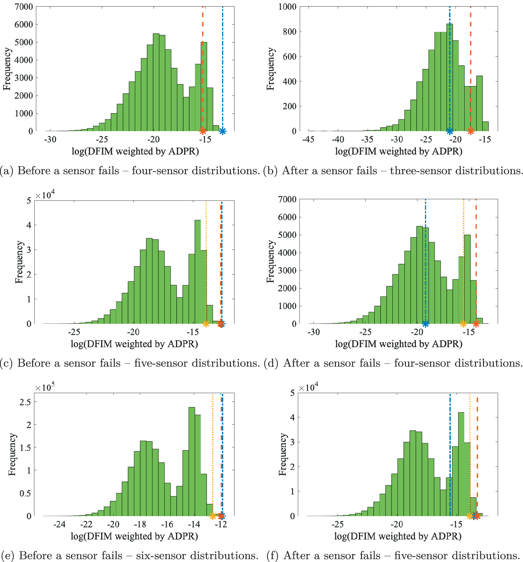
Comparison of the SSC results of a GA, an improved-fail-safe GA, and an improved-fail-safe with redundancy GA, with the ES results.

Comparison of the SSC-ADPR results of a GA, an improved-fail-safe GA, and an improved-fail-safe with redundancy GA, with the ES results.

Before comparing the optimal results obtained by the two applied search algorithms, it should be noted that: (a) when comparing the optimal results corresponding to an ES and a GA obtained by classical SPO (marked with a blue dash-dotted line and a blue asterisk, respectively), the fitness value before the sensor failure should be used, as shown in the left sub-figures and marked in blue. This choice is because, for classical SPO, the sensor deployment is optimized according to the fitness of the mother distribution. (b) For the optimal results obtained by the other two optimization strategies, it is necessary to compare the optimal fitness values corresponding to two search algorithms after the failure of the marked sensor, as shown in the right sub-figures and marked with orange or yellow dash-dotted lines and asterisks, because, for these two SPO, the sensor deployment is optimized on the worst child fitness.
It can be seen that the optimal sensor deployments with three to five sensors obtained by the ES and the GA are the same. Furthermore, the fitness, fail-safe fitness, or fail-safe with redundancy fitness of the optimal sensor combinations with six sensors obtained by both search algorithms are close to each other. Thus, the GA adopted here is effective for searching out optimization results.
To check the performance of the sensor distributions obtained by the fail-safe SPO and the fail-safe with redundancy SPO, different histograms of the fitness values corresponding to all sensor distributions with the same number of sensors from an ES are also plotted in Figures 5–8 in green.
For the fail-safe SPO strategy, the expected result is that the performance of the sensor system before any sensor failure is very similar between the classical and fail-safe methods, while the worst-case performance of the sensor system obtained by the fail-safe method is better than that of the sensor system corresponding to the classical method after a critical sensor failure. This phenomenon can be observed particularly in four pairs of Figures 5a,b, 6c,d,e,f, and 8e,f.
Overall, it can be found that the obtained improved-fail-safe sensor distribution provides good performance when all sensors are working normally. Besides, it also ensures that acceptable performance can be maintained when any sensor fails. For the case when the optimal improved-fail-safe sensor distribution (in orange) is the same as the optimal sensor distribution with the largest fitness (in blue), the obtained fail-safe sensor distribution does not compromise the system performance before any sensor fails, as demonstrated in Figures 5c,d and 8a,b.
When it comes to the fail-safe with redundancy SPO, results in Figures 5–8 indicate that when the number of sensors is greater than 5, the performance corresponding to its optimal result changes the least before and after the sensor failure; this means that the redundant sensor is useful to increase the sensor system’s ability to withstand sensor failures. However, for this kind of SPO, a pair of sensors is placed at the same position, which will collect the same information. Therefore, although the sensor failure has the least effect on the performance of the sensor distribution, the optimal sensor distribution found via this optimization strategy almost always has the worst performance before and after a sensor fails compared with the other optimization approaches.
Note that the two improved fail-safe strategies cannot directly trade off the fitness of the mother distribution and the fail-safe fitness of the child distribution. Although the GA results in Figure 7e,f show the trade-off possibility, a possible reason for the phenomenon shown in Figure 7e,f is that the GA fails to find the optimal fail-safe sensor distribution, but instead finds a sub-optimal fail-safe sensor distribution, which sacrifices less performance of the sensor system without a failed sensor to consider the effect of senor failure.
5.4. Optimal sensor distribution comparisons
In this part, the optimal sensor distributions with six and eight sensors searched by an ES and a GA respectively are plotted in Figures 9 and 11 to analyze the distribution characteristics of sensors obtained using different optimization objectives. For each optimization objective, the sensor distributions obtained by the two search algorithms are similar. This phenomenon also reflects the reliability of GA results. So far, it can be said that a GA can be used to search for a reliable optimization result when optimizing a sensor system that is too complex for ES.
Comparison of optimal six-sensor distributions obtained by three ES-based optimization strategies combined with four optimization objectives. The selected sensor locations are marked in red. The sensors whose failure will lead to the worst and the second-worst child fitness are marked in blue and green. FR, fail-safe; FSR, fail-safe with redundancy.

The specific features of optimal distributions included are as follows: (a) By comparing the optimal sensor distributions considering ADPR with the distribution of locations with larger ADPR values shown in Figure 10, it can be seen that the addition of signal strength in the fitness will have a certain impact on the result but it is limited. (b) Considering the signal strength in the objective function has a greater impact on the optimization results based on SSC than those based on DFIM. By comparing Figures 5 and 7, it can be seen that a possible reason for this phenomenon is that the difference in DFIM corresponding to different sensor combinations is larger than the difference in SSC. Therefore, the addition of ADPR into the optimization objective has a more limited impact on the ranking of DFIM-based fitness. (c) As expected, the optimal sensor distribution corresponding to SSC fitness is closer to the damage points of interest. (d) Fail-safe SPO makes the selected sensors more evenly dispersed on the structure to be monitored. This kind of deployment explains to a certain extent why the performance of the fail-safe sensor distribution is good, both before and after the sensor failure.
Rescaled ADPR corresponding to 36 candidate sensor locations. The first six maximum values are marked in red, and the next two are marked in magenta.

Comparison of optimal eight-sensor distributions obtained by three GA-based optimization strategies combined with four optimization objectives.

6. Conclusions
This article aims to design an optimization technique considering the effect of sensor failure for a wired sensor system. Two SPO strategies, including the improved-fail-safe SPO and the improved-fail-safe SPO with redundancy, are proposed for modal identification and damage identification issues. From three perspectives (the accuracy of the target modal-coordinate estimate, the vibration energy, and the information on the damage of interest), four objective functions based on model parameters, including the DFIM, the DFIM-ADPR, the SSC, and the SSC-ADPR, are adopted and combined with two search algorithms, including a deterministic algorithm—ES and a stochastic algorithm—GA to obtain the optimal sensor layouts. Among them, SSC is used as an optimization objective for sensor placement for the first time, which is inherently immune to the information redundancy and interaction issue.
A case study of a glider wing is demonstrated. By comparing with the classical SPO, it has been found that the improved-fail-safe sensor distribution can provide good performance when all sensors are working normally and guarantee good performance when any sensor fails. Furthermore, the redundant sensor helps enhance the sensor system’s ability to withstand sensor failures, but the overall performance is not attractive; this shows that it is not advisable to place redundant sensors in a wired sensor system to avoid the worst system performance because of damage to a key sensor. In the case of a certain number of sensors, the improved fail-safe SPO can make the most effective use of sensor resources by placing the sensors in different locations.
In future work, in addition to mode shapes, other data types will be involved, including time-domain data and frequency-domain data, to further explore the feasibility and characteristics of the improved fail-safe SPO technique. If the data are suitable, the three optimization methods can be compared in the presence of uncertainty in the optimization process, and a cost-related optimization objective or multi-objective optimization can be considered. Cost-related evaluation studies could also be conducted in the future, to determine the number of sensors allowed to fail without any remedial action for a practical project.
Competing Interests
The authors declare no competing interests exist.
Acknowledgment
We thank Robin S. Mills for providing technical assistance for testing.
Supplementary Materials
To view supplementary material for this article, please visit http://doi.org/10.1017/dce.2022.27.
Data Availability Statement
The data and codes that support the findings of this study are openly available in the GitHub repository at https://github.com/TingnaW/Fail-safe_SPO_codes.
Author Contributions
Conceptualization: T.W., K.W.; Data curation: T.W., R.J.B.; Data visualization: T.W.; Formal analysis: T.W.; Funding acquisition: R.J.B., D.J.W., K.W.; Investigation: T.W.; Methodology: T.W., K.W.; Writing—original draft: T.W.; Writing—review and editing: T.W., D.J.W., K.W.
Funding Statement
The authors would like to acknowledge the support of Siemens Gamesa and UK EPSRC via grant number EP/R004900/1. This research made use of The Laboratory for Verification and Validation (LVV) which was funded by the EPSRC (grant numbers EP/J013714/1 and EP/N010884/1) and the University of Sheffield. For the purpose of open access, the author(s) has/have applied a Creative Commons Attribution (CC BY) licence to any Author Accepted Manuscript version arising.


 Open access


Comments
No Comments have been published for this article.